Multiscale Quantile Regression with Local Error Control

Abstract

For robust and efficient detection of change points, we introduce a novel methodology MUSCLE (multiscale quantile segmentation controlling local error) that partitions serial data into multiple segments, each sharing a common quantile. It leverages multiple tests for quantile changes over different scales and locations, and variational estimation. Unlike the often adopted global error control, MUSCLE focuses on local errors defined on individual segments, significantly improving detection power in finding change points. Meanwhile, due to the built-in model complexity penalty, it enjoys the finite sample guarantee that its false discovery rate (or the expected proportion of falsely detected change points) is upper bounded by its unique tuning parameter. Further, we obtain the consistency and the localisation error rates in estimating change points, under mild signal-to-noise-ratio conditions. Both match (up to log factors) the minimax optimality results in the Gaussian setup. All theories hold under the only distributional assumption of serial independence. Incorporating the wavelet tree data structure, we develop an efficient dynamic programming algorithm for computing MUSCLE. Extensive simulations as well as real data applications in electrophysiology and geophysics demonstrate its competitiveness and effectiveness. An implementation via R package muscle is available from GitHub.

Keywords: change points, false discovery rate, minimax optimality, multiscale method, robust segmentation, wavelet tree

1 Introduction

Detecting and localising abrupt changes in time series data has been a vibrant area of research in statistics and related fields since its early study (e.g. Wald, , 1945; Page, , 1955). For a comprehensive overview, refer to Niu et al., (2016) and Truong et al., (2020). These methods find applications across a wide range of fields, for example, bioinformatics (Futschik et al., , 2014), ecosystem ecology (Berdugo et al., , 2020), electrophysiology (Pein et al., , 2017, 2018), epidemiology (Dehning et al., , 2020), economics and finance (Russell and Rambaccussing, , 2019), molecular biophysics (Fan et al., , 2015) and social sciences (Liu et al., , 2013). The extensive applications have sparked an explosion of methods for detecting changes in the recent literature. Notable examples include the regularised maximum likelihood estimation (e.g. Boysen et al., , 2009; Harchaoui and Lévy-Leduc, , 2010; Killick et al., , 2012; Du et al., , 2016; Maidstone et al., , 2017), the multiscale approaches (e.g. Frick et al., , 2014; Li et al., , 2016; Pein et al., , 2017; Eichinger and Kirch, , 2018) and binary segmentation type methods (e.g. Vostrikova, , 1981; Fryzlewicz, , 2014; Baranowski et al., , 2019; Fang et al., , 2020; Kovács et al., , 2023), to name only a few.

There is, however, a relative lack of understanding on whether detected change points truly reflect genuine structural changes, arise from random fluctuations, or result from statistical modelling errors. The distinction poses a delicate challenge in practical applications, necessitating an in-depth grasp of the data as well as the employed change point detection methods. In pursuit of an automatic and versatile solution, we introduce here a robust change point estimator, named MUSCLE (Multiscale qUantile Segmentation Controlling Local Error; see Section 2), that focuses on the recovery of genuine structural changes while maintaining high detection power as if a strong statistical model were faithfully available. Importantly, we adopt a quantile segmentation perspective and focus on local error control instead of often considered global error control, as explained in detail below.

1.1 Quantile segmentation model

Following Vanegas et al., (2022) and Fryzlewicz, (2024), we inspect the underlying structural changes in terms of changes in quantiles.

Model 1 (Quantile segmentation model).

Let $\beta\in(0,1)$ and $f_{\beta}:[0,1)\to\mathbb{R}$ be a piecewise constant function

$$f_{\beta}\;=\;\sum_{k=0}^{K}\theta_{k}\mathbbm{1}_{[\tau_{k},\tau_{k+1})},\qquad\text{with }\theta_{k}\neq\theta_{k+1},\,0=\tau_{0}<\cdots<\tau_{K+1}=1,$$

where the number of change points $K$, the locations of change points $\tau_{k}$ and the segment values $\theta_{k}$ are all unknown. Assume that the observations $Z=(Z_{1},\dots,Z_{n})$ are independent random variables with their $\beta$-quantiles equal to $f_{\beta}(x_{i})$, i.e.,

$$\mathbb{P}\bigl{(}Z_{i}\leq f_{\beta}(x_{i})\bigr{)}=\beta\quad\text{ or }\quad F_{i}\bigl{(}f_{\beta}(x_{i})\bigr{)}=\beta,$$

where $x_{i}=(i-1)/n$, $i=1,\ldots,n$, are equidistant sampling points, and $F_{i}$ the distribution function of $Z_{i}$.

Equivalently, Model 1 can be written into a typical form of additive noise model

$$Z_{i}=f_{\beta}\left(x_{i}\right)+\varepsilon_{i},\quad\quad i=1,\dots,n,$$ (1)

where noises $\varepsilon_{i}$ are independent with their $\beta$-quantiles equal to zero. For instance, the choice of $\beta=0.5$ corresponds to the median segmentation regression. The subscript $\beta$ will be suppressed whenever there is no ambiguity. Since our aim is to provide a $\beta$-quantile segmentation, with an arbitrary yet fixed $\beta\in(0,1)$, we do not consider $\beta$ as a tuning parameter.

We stress that there are no distributional assumptions on observations $Z_{i}$ or equivalently on the additive noises $\varepsilon_{i}$, other than the statistical independence. This in particular allows arbitrarily heavy tailed, skewed or heterogeneous noise distributions, outliers, or a mixture of them (see Section 5.1.1 for some examples). It will further allow $\varepsilon_{i}$ to have a discrete distribution, provided that $\mathbb{P}(\varepsilon_{i}\leq 0)=\beta$. In addition, if we consider multiple quantiles with different choices of $\beta$ in Model 1, we may be able to detect distributional changes in the observations (see Section 5.1.2 and Figure 6).

1.2 Local error control

As a motivating example, we consider a particular instance of the additive noise model (1) with sample size $n=400$, the signal $f\equiv f_{\beta}=2\cdot\mathbbm{1}_{[0.05,0.1)}-2\cdot\mathbbm{1}_{[0.6,0.725)}$, and the independent centred (i.e. $\beta=0.5$) noises $\varepsilon_{i}\sim\mathcal{N}(0,1)$ if $1\leq i\leq 100$ and $\varepsilon_{i}\sim t_{3}/(2\sqrt{3})$ if $101\leq i\leq 400$. Here and below $\mathcal{N}(\mu,\sigma^{2})$ denotes the normal distribution with mean $\mu$ and variance $\sigma^{2}$, and $t_{m}$ the Student’s $t$ distribution of $m$ degrees of freedom. In order to see the influence of the choice of data window, we apply the proposed MUSCLE and several recent proposals (Haynes et al., , 2017; Baranowski et al., , 2019; Fearnhead and Rigaill, , 2019; Madrid Padilla et al., , 2021; Vanegas et al., , 2022; Fryzlewicz, , 2024) of robust or nonparametric segmentation methods on the first 80 observations and also on the whole data of 400 observations, see Figure 1. As shown, the considered methods except MUSCLE give different estimates (marked by solid and dashed lines) of the signal $f$ on the interval $[0,\,80/n)$ when applied to the two different windows of the data. This reflects the often unspoken fact that the choice of data window is actually a hyper-parameter in real data applications (cf. Ermshaus et al., , 2023). The reason behind is that data analysis methods are often globally tuned for the whole window of data.

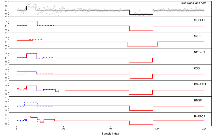
Figure 1: Influence of data windowing on segmentation methods. The top panel plots the true signal (line) and data (crosses). The lower panels show the segmentation results using only the first 80 samples (dashed line) and using the whole data of 400 samples (solid line), by the proposed MUSCLE, MQS (Vanegas et al., , 2022), NOT-HT (Baranowski et al., , 2019, the heavy tailed version), KSD (Madrid Padilla et al., , 2021), ED-PELT (Haynes et al., , 2017), RNSP (Fryzlewicz, , 2024) and R-FPOP (Fearnhead and Rigaill, , 2019), respectively. The vertical dashed line is at $n=80$ (marking the first 80 samples).

The distinctive feature of MUSCLE, being stable across different data windows, is mainly due to its control of local errors on individual segments. Namely, it controls separately the error of reporting any false detection of change points over all local intervals within every estimated segment. The stability to choices of data windows not only simplifies real data analysis in applications, but also has important implications on computational efficiency and statistical power. For instance, we can split the data into several pieces of equally fixed lengths, apply MUSCLE on each piece of data separately, and then merge the results to obtain the final estimate for the whole data. This splitting-merging approach results in a computation time that increases linearly with the sample size $n$, and also allows a linear speedup in parallel computing with multiple computing units (see Section 4 and, in particular, Remark 4). Also, as a weaker criterion compared to the global error control, the local error control would allow an enhanced detection power in finding change points, though it might suffer from the tendency of including false positives (i.e., falsely detected change points). Nevertheless, MUSCLE addresses this issue through a built-in penalty on model complexity, and allows to adjust the control on false positives by its only tuning parameter. Besides, the local error control is particularly suited to the problem of change point detection, since a change point is essentially a local feature on an interval consisting of its two adjacent segments.

1.3 Our contribution and related work

Under the quantile segmentation model (i.e., Model 1), the proposed MUSCLE scans over intervals of varying scales and locations in search for changes in quantile, and estimates the underlying quantile function in the framework of variational multiscale estimation (Haltmeier et al., , 2022). It penalises the model complexity in terms of the number of change points, under a convex polytope constraint that builds upon a meticulously crafted multiscale statistics towards local error control on each individual segment. Due to this construction, MUSCLE is robust and has a high detection power at the same time, as supported by numerous simulations and real data analyses (see Section 5). Moreover, we showcase two extensions of MUSCLE to the detection of changes in distribution (M-MUSCLE; Section 5.1.2) and to a dependent scenario (D-MUSCLE; Section 5.2.2).

Let $\widehat{f}$ be the MUSCLE estimator and $\widehat{K}$ its number of estimated change points, and assume Model 1. We have established the finite sample guarantee (Theorem 5) on falsely detected change points

$$\mathbb{E}\left[\frac{\max\{\widehat{K}-K,0\}}{\max\{\widehat{K},1\}}\right]\;\leq\;\alpha$$

where $\alpha\in(0,1)$ is the only tuning parameter of MUSCLE. This bound, together with the fact that a larger $\alpha$ often leads to a larger $\widehat{K}$, allows data analysts to tune MUSCLE according to their needs in real data applications.

Besides, we have derived the consistency (Theorem 3) and the localisation errors (Theorem 4) of MUSCLE in estimating change points provided that, for some large enough constant $C$,

$$n\cdot\min\{\tau_{k}-\tau_{k-1},\tau_{k+1}-\tau_{k}\}\cdot\min_{i\in[\tau_{k-1},\tau_{k+1})}\left|F_{i}\left(\tfrac{\theta_{k}+\theta_{k-1}}{2}\right)-\beta\right|^{2}\;\geq\;C\log n,\qquad k=1,\ldots,K,$$ (2)

the left hand side of which measures the detectability of change points $\tau_{k}$. These results match, up to log factors, the results of minimax optimality in the Gaussian setup (Verzelen et al., , 2023). Further, our consistency result follows from the stronger results of exponential bounds on under- and overestimation errors (Theorems 1 and 2).

Computationally, we have developed an efficient dynamic programming algorithm for MUSCLE, which has a worst-case computational complexity of $O(n^{3}\log^{2}n)$ and requires $O(n\log n)$ memory (see Section 4). The algorithm’s key components include the wavelet tree (Navarro, , 2014) data structure and the use of a sparse collection of intervals at different scales and locations (Walther and Perry, , 2022). In contrast, the commonly used linear data structure would increase the computational complexity by a factor of $O(n)$, and the double heap structure, as used in Vanegas et al., (2022), would result in a worst-case memory requirement of $O(n^{2})$. The use of all intervals would also lead to an additional factor of $O(n)$ in the computational complexity.

The proposed MUSCLE belongs to the family of multiscale approaches (initiated by Frick et al., , 2014), among which the most closely related methods are FDRSeg (Li et al., , 2016) and MQS (Vanegas et al., , 2022). MUSCLE extends FDRSeg, designed for the standard Gaussian noises, to handle general independent noises, and significantly enhances the detection power of MQS by switching to local error control. Further, the statistical results in this paper are sharper and more general compared to the aforementioned two papers. More precisely, we have improved the upper bound of false discovery rate in Li et al., (2016) from $2\alpha/(1-\alpha)$ to $\alpha$, while also admitting of general distributions beyond Gaussian, by employing a completely different proof technique (see Section 3.2). In comparison with Vanegas et al., (2022), we have refined the overestimation bound on the number of change points (Theorem 2), derived a quantitative estimate of the tail probability of multiscale statistics (Lemma 10 in Appendix A), and reformulated the detection condition into a weaker form (2), which allows frequent large jumps and rare small jumps over long segments to occur at the same time. These improvements are mainly due to the use of strengthened technical inequalities (e.g., Talagrand’s concentration inequality for convex distances) and a minor adjustment of multiscale statistics (see footnote 1 on page 1). In addition, the optimisation problem defining MUSCLE poses notable challenges compared to FDRSeg and MQS. However, by incorporating the wavelet tree data structure, we are able to achieve nearly (up to a log factor) the same worst-case computational complexity as FDRSeg.

Further related works include robust segmentation methods. Baranowski et al., (2019), though primarily considered Gaussian setups, suggested a heavy tail extension (NOT-HT) that truncates the data into $\pm 1$ by a certain sign transform and then treats the truncated data as if they were Gaussian distributed. Fryzlewicz, (2024) further developed this idea, and introduced Robust Narrowest Significance Pursuit (RNSP), which utilises a sign-multiresolution norm. The statistical guarantees of RNSP are provided in the additive noise model (1) with additional assumption that noises are independently and identically distributed (i.i.d.), continuous random variables. From a penalised M-estimation perspective, Fearnhead and Rigaill, (2019) proposed R-FPOP employing Tukey’s biweight loss, and derived asymptotic properties for a restrictive scenario with fixed change points. Another line of related works are nonparametric change point methods, which assume that the observations are piecewise i.i.d. (a slightly stronger model than Model 1). Matteson and James, (2014) introduced a hierarchical clustering-type method based on the energy distance between probability measures, and proved consistency results (with no rates) under additional moment conditions. Utilising a weighted Kullback–Leibler divergence, Zou et al., (2014) proposed Nonparametric Multiple Change-point Detection (NMCD), together with consistency and localisation rates of change points. As a computational speedup variant of NMCD, Haynes et al., (2017) introduced ED-PELT by simplifying the involved cost function through discrete approximation. Madrid Padilla et al., (2021) developed a CUSUM procedure (KSD) based on the Kolmogorov–Smirnov distance, and established better statistical guarantees than Zou et al., (2014), but requiring prior knowledge on the minimum segment length. We include a large selection of the above methods in our comparison stduy on simulated and real world data (see Section 5).

1.4 Outline and notation

Section 2 introduces MUSCLE, a novel methodology for multiple change point segmentation under Model 1. Section 3 delves into the statistical theories of MUSCLE, including consistency, localisation error rates of change points and finite sample guarantees on falsely detected change points. Section 4 discusses the computation of MUSCLE. Section 5 presents simulation studies and real data applications. The paper concludes with a discussion in Section 6. Additional material and proofs are given in the Appendix. The R package muscle implementing MUSCLE and its variants is available from https://github.com/liuzhi1993/muscle.

By convention, all intervals in this paper are of form $[a,b)$, where $a,b\in\mathbb{R}$ and $a<b$. For sequences $\{a_{m}\}$ and $\{b_{m}\}$ of positive numbers, we write $a_{m}\lesssim b_{m}$ if $a_{m}\leq Cb_{m}$ for some finite constant $C>0$. If $a_{m}\lesssim b_{m}$ and $b_{m}\lesssim a_{m}$, we write $a_{m}\asymp b_{m}$. We write $X\overset{\mathcal{D}}{=}Y$ to indicate that random variables $X$ and $Y$ have the same distribution. We write $(x)_{+}=\max\{x,0\}$ for $x\in\mathbb{R}$. By $\sqcup$ we denote the disjoint union. By $\#S$ we denote the cardinality of the a $S$.

2 Methodology

2.1 Multiscale test on a segment

Assume that observations $Z_{1},\ldots,Z_{n}$ are from Model 1, and let interval $I\in\{[\tau_{k},\tau_{k+1}):k=0,\ldots,K\}$ be an arbitrary segment of the quantile function $f\equiv f_{\beta}$. It follows that $\{Z_{i}:x_{i}\equiv(i-1)/n\in I\}$ are independent and have the common $\beta$-quantile, whereas their distributions $F_{i}$ may not be identical. Towards a uniform treatment, we transform the data into simple binary samples as

$$W_{i}\coloneqq W_{i}(Z_{i},\theta)\coloneqq\mathbbm{1}_{\{Z_{i}\leq\theta\}},\quad i=1,\dots,n.$$

If $\theta$ equals the common $\beta$-quantile of $\{Z_{i}:x_{i}\in I\}$, the transformed samples $\{W_{i}:x_{i}\in I\}$ are i.i.d. Bernoulli random variables with mean $\beta$. The condition of $\theta$ equal to the common quantile can be verified using the data, when viewed as a hypothesis testing problem. We tackle the testing problem by multiscale procedures, which build on a delicate combination of multiple simple tests, and are known to be optimal in the minimax sense (see e.g. Dümbgen and Spokoiny, , 2001; Frick et al., , 2014). More specifically, we consider the testing problems, for intervals $J\subseteq I$,

$$H_{J}:\mathbb{P}(Z_{i}\leq\theta)=\beta,\quad x_{i}\in J\qquad\text{versus}\qquad A_{J}:\mathbb{P}(Z_{i}\leq\theta)\neq\beta,\quad x_{i}\in J.$$

For each of them, we employ the likelihood ratio test statistic

$$L_{J}(Z,\theta)=\lvert J\rvert\left[\overline{W}_{J}\log\left(\frac{\overline{W}_{J}}{\beta}\right)+(1-\overline{W}_{J})\log\left(\frac{1-\overline{W}_{J}}{1-\beta}\right)\right],$$

where $\lvert J\rvert=\#\{i:x_{i}\in J\}$ and $\overline{W}_{J}=\left(\sum_{i\in J}W_{i}\right)/\lvert J\rvert$. The null hypothesis $H_{J}$ is reject if $L_{J}$ exceeds a certain critical value. As in Frick et al., (2014), we incorporate all of such tests with the control of family-wise error, and balance the detection powers over different scales of $\lvert J\rvert$. This leads to the multiscale statistic with scale penalty

$$T_{I}(Z,\theta)\;=\;\underset{J\subseteq{I}}{\max}\sqrt{2L_{J}(Z,\theta)}-\sqrt{2\log\left(\frac{e\lvert I\rvert}{\lvert J\rvert}\right)}.$$ (3)

To calibrate the family-wise error rate, we introduce the critical value

$$q_{\alpha}(\lvert I\rvert)\;=\;\min\left\{q:\mathbb{P}\bigl{(}T_{I}(Z,\theta)>q\bigm{|}H_{J},J\subseteq I\bigr{)}\leq\alpha\right\},$$ (4)

which is also referred to as a local quantile on the segment $I$. Note that $\{W_{i}(Z_{i},\theta)\,:\,x_{i}\in I\}$ are i.i.d. Bernoulli distributed with mean $\beta$, under all $H_{J}$ for $J\subseteq I$. Thus, the distribution of $T_{I}(Z,\theta)$ conditioned on all $H_{J}$ for $J\subseteq I$ is known and equal to the maximum of dependent and transformed Bernoulli distributions. A simple and explicit form of $q_{\alpha}(\lvert I\rvert)$ is not yet available, but we can estimate it by Monte–Carlo simulations. Thus, the decision problem of whether $\{Z_{i}:x_{i}\in I\}$ have the same $\beta$-quantile equal to $\theta$ can be addressed by the multiscale test $\mathbbm{1}_{\{T_{I}(Z,\theta)>q_{\alpha}(\lvert I\rvert)\}}$ with the type I error no more than $\alpha$.

Remark 1 (Multiscale statistics).

The scale penalty term $\sqrt{2\log(e\lvert I\rvert/\lvert J\rvert})$ in (3) is motivated by the fact that $\max_{J:\lvert J\rvert=m}\sqrt{2L_{J}(Z,\theta)}$ concentrates asymptotically around $\sqrt{2\log(\lvert I\rvert/m)}$, see e.g. Kabluchko, (2011). This scale penalty not only standardises the influence of scale $\lvert J\rvert$ but also ensures the asymptotic tightness of $T_{I}$ as $\lvert I\rvert\to\infty$. The form of scale penalties is though not unique. Alternative forms can be found e.g. in Walther and Perry, (2022). Moreover, the distribution of $T_{I}(Z,\theta)$ conditioned on $\cap_{J\subseteq I}H_{J}$ converges weakly to an almost surely finite random variable as $\lvert I\rvert\to\infty$ under a minor restriction on the smallest scale, namely, $\lvert J\rvert\gg\log^{3}\lvert I\rvert$, see e.g. Frick et al., (2014) and Dümbgen and Spokoiny, (2001). It follows readily that $\limsup_{\lvert I\rvert\to\infty}q_{\alpha}(\lvert I\rvert)<\infty$ for any fixed $\alpha\in(0,1)$. Further, we have shown an explicit upper bound in form of $\limsup_{\lvert I\rvert\to\infty}q_{\alpha}(\lvert I\rvert)\lesssim\sqrt{-\log\alpha}$, see Lemma 10 in Appendix A. This upper bound may serve as an estimate of $q_{\alpha}(\lvert I\rvert)$ particularly when $\lvert I\rvert$ is so large that Monte–Carlo simulations become computationally unaffordable. Alternatively, we might be able to approximate $q_{\alpha}(\lvert I\rvert)$ in a deterministic manner, following ideas in Fang et al., (2020). Their results, however, do not apply directly in our case, mainly due to the presence of the scale penalty term. The exploration of this possibility is an interesting avenue of future research.

2.2 The proposed MUSCLE

A reasonable candidate $g$ for the recovery of the quantile function $f$ in Model 1 should pass the multiscale tests on individual segments. Thus, we restrict ourselves to functions lying in the multiscale side-constraint

$$\mathcal{C}_{k}\coloneqq\left\{g=\sum_{j=0}^{k}\theta_{j}\mathbbm{1}_{{I}_{j}}\;:\;T_{\accentset{\circ}{I}_{j}}(Z,\theta_{j})-q_{\alpha}(\lvert\accentset{\circ}{I}_{j}\rvert)\leq 0,\,j=0,\dots,k\text{ and }\bigsqcup_{j=0}^{k}I_{j}=[0,1)\right\},$$ (5)

where $\accentset{\circ}{I}$ denotes the interior of interval $I$. Note that in this particular form of $\mathcal{C}_{k}$ we control the type I error locally on every segment $I_{i}$. Further, to avoid overfitting to the data, we minimise the complexity of candidates, which is measured by the number of change points, and define

$$\widehat{K}\coloneqq\min\bigl{\{}k\in\mathbbm{N}\cup\{0\}\,:\,\mathcal{C}_{k}\neq\emptyset\bigr{\}}.$$ (6)

We thus introduce Multiscale qUantile Segmentation Controlling Local Errors (MUSCLE) as the candidate in $C_{\widehat{K}}$ that fits best to the data, namely,

$$\widehat{f}\;\in\;\underset{g\in\mathcal{C}_{\widehat{K}}}{\arg\min}\,\sum_{i=1}^{n}\bigl{(}Z_{i}-g(x_{i})\bigr{)}\bigl{(}\beta-\mathbbm{1}_{\{Z_{i}\leq g(x_{i})\}}\bigr{)}.$$ (7)

The fitness to the data is quantified with respect to the asymmetric absolute deviation loss (or check loss), which is typically employed in defining quantiles (see e.g. Koenker, , 2005).

Note that $\tilde{f}=\sum_{i=1}^{n}Z_{i}\mathbbm{1}_{[x_{i},x_{i+1})}$ clearly lies in $\mathcal{C}_{n-1}$, so $\widehat{K}$ is finite and takes values in $\{0,1,\ldots,n-1\}$. Thus $\mathcal{C}_{\widehat{K}}\neq\emptyset$ and consequently a solution $\widehat{f}$ of (7) always exists. Owing to the specific structure of the optimisation problem, $\widehat{f}$ can be efficiently computed in the dynamic programming framework (see Section 4).

2.3 Comparison with global error control

A distinctive feature of MUSCLE is the control of local errors on individual segments, which is built in the construction of the multiscale side-constraint $\mathcal{C}_{k}$ in (5). To further understand the strength of local error control, we compare MUSCLE with MQS (Multiscale Quantile Segmentation; Vanegas et al., , 2022), a similar method but with the global error control. The distinction between these two methods lies in the construction of multiscale side-constraint. MQS searches for a candidate with minimum number of change points and minimum asymmetric absolute deviation loss over

$$\mathcal{C}_{k}^{0}\coloneqq\left\{g=\sum_{j=0}^{k}\theta_{j}\mathbbm{1}_{I_{j}}\;:\;{T}^{0}_{I_{j}}(Z,\theta_{j})-q_{\tilde{\alpha}}(n)\leq 0,\,j=0,\dots,k\text{ and }\bigsqcup_{j=0}^{k}I_{j}=[0,1)\right\},$$

where $T_{I}^{0}(Z,\theta)\coloneqq{\max}_{J\subseteq I}\sqrt{2L_{J}(W,\theta)}-\sqrt{2\log\left({en}/{\lvert J\rvert}\right)}$ and $\tilde{\alpha}\in(0,1)$ is the tuning parameter. Compared to (5), the difference in quantiles and penalties arises from the control of different errors. The global error control of MQS ensures that the true quantile function $f$ lies in $\mathcal{C}_{K}^{0}$ with probability no less than $1-\tilde{\alpha}$. By contrast, the local error control of MUSCLE guarantees that each segment of the true quantile function $f$ satisfies the side-constraint with probability no less than $1-\alpha$, which further implies that $f$ lies in $\mathcal{C}_{K}$ with probability no less than $(1-\alpha)^{K+1}$. Then, unless $\tilde{\alpha}\geq 1-(1-\alpha)^{K+1}\approx(K+1)\alpha$, the multiscale side-constraint $\mathcal{C}_{K}$ is generally smaller than $\mathcal{C}^{0}_{K}$. As a consequence, MUSCLE is likely to report more change points than MQS. Thus, the local error control enables MUSCLE to overcome the conservativeness (i.e., the tendency to miss true change points) that is often observed for multiscale segmentation methods.

As a simulation study, we consider the recovery of the teeth function that contains $K=80$ change points under the additive noise model (1), where the noises are scaled $t_{3}$-distributed with standard deviation equal to one. The simulation results are given in Figure 2 and Table 1. Clearly, MUSCLE ($\alpha=0.3$) recovers nicely the number and the locations of change points, while MQS ($\tilde{\alpha}=0.3$) severely underestimates the number of change points. To enhance the detection power of MQS, we adjust $\tilde{\alpha}=1-(1-0.3)^{81}\approx 0.999$. This adjustment significantly improves MQS in the estimation of $K$, bringing its performance closer to MUSCLE, but at the expense of nearly no statistical guarantee. Still, MQS with such a large $\tilde{\alpha}$ underperforms MUSCLE in estimating the change point locations as well as the whole signal. See Section 5.1 (and also Section 1.2) for further comparisons.

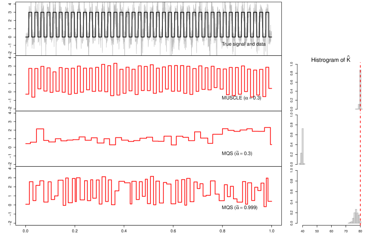
Figure 2: Comparison of the proposed MUSCLE and MQS (Vanegas et al., , 2022). The true signal (black line), which is a teeth function, and data (gray line; $2000$ samples) are shown in the top panel. The estimates by MUSCLE ($\alpha=0.3$), MQS ($\tilde{\alpha}=0.3$) and MQS ($\tilde{\alpha}=0.999$) are plotted in lower panels. The performance of each method, over $200$ repetitions, in estimating the number of change points is visualised by histograms on the right hand side. The true number of change points $K=80$ is marked by a vertical dashed line.

Table 1: Comparison of MQS and MUSCLE in the setup of Figure 2. For each criterion, the average value and the standard deviation (in brackets), over 200 repetitions, are presented. Here $d_{H}$ denotes the Hausdorff distance between estimated and true change points, MISE the mean integrated squared error of $\widehat{f}$ and MIAE the mean integrated absolute error. Their formal definitions are given in (12), and in (23) and (24) in Appendix B, respectively.

Methods	$\widehat{K}$	$d_{H}$	MISE	MIAE
MUSCLE ($\alpha=0.3$)	$80\;(0.4)$	$0.001\;(0.0030)$	$0.1\;(0.041)$	$0.2\;(0.020)$
MQS ($\tilde{\alpha}=0.3$)	$40\;(0.5)$	$0.015\;(0.0037)$	$2.7\;(0.065)$	$1.4\;(0.008)$
MQS ($\tilde{\alpha}=0.999$)	$77\;(1.6)$	$0.008\;(0.0006)$	$1.8\;(0.108)$	$0.9\;(0.057)$

3 Statistical Properties

Here we provide statistical guarantees on the proposed MUSCLE under Model 1. In all of the theoretical results, we allow the quantile function $f$ as well as distribution functions $F_{i}$ in Model 1 to change as sample size varies. We use subscript $n$ to emphasise such a dependence whenever needed.

3.1 Consistency and localisation rates

Following Vanegas et al., (2022), we measure the changes in quantiles by the quantile jump function.

Definition 1 (Vanegas et al., , 2022).

Let $F$ be a distribution function and $\beta\in(0,1)$. The $\beta$-quantile of $F$ is given by $F^{-1}(\beta)\coloneqq\inf\{x:F(x)\geq\beta\}.$ The quantile jump function is defined by

$$\xi_{F,\beta}(\delta)\coloneqq\left|F\bigl{(}F^{-1}(\beta)+\delta\bigr{)}-\beta\right|,\qquad\text{for}\quad\delta\in\mathbb{R}.$$

Example 1 (Distribution with continuous density).

Let $F$ be a distribution function that is continuously differentiable. Then for any $\beta\in(0,1)$ we have

$$\xi_{F,\beta}(\delta)=\lvert F(F^{-1}(\beta)+\delta)-\beta\rvert=\lvert F(F^{-1}(\beta)+\delta)-F(F^{-1}(\beta))\rvert=F^{\prime}\bigl{(}F^{-1}(\beta)\bigr{)}\delta+o(\delta).$$

In particular, in the Gaussian model with changing means, the quantile jump function with $\beta=0.5$ satisfies

$$\xi_{\Phi,0.5}(\delta)\;\approx\;\varphi(0)\delta\;=\;\frac{1}{\sqrt{2\pi}}\delta\;\approx\;\frac{2}{5}\delta,$$

where $\Phi$ and $\varphi$ denote the distribution function and the density of standard normal distribution, respectively.

Recall the notation in Model 1. For $k=1,\dots,K$, let $\lambda_{k}=\min\{\tau_{k}-\tau_{k-1},\tau_{k+1}-\tau_{k}\}$ and $I_{k}=(\tau_{k}-\lambda_{k}/2,\tau_{k}+\lambda_{k}/2)$, and define

$$F_{\min,k}\;=\;\underset{i:x_{i}\in I_{k}}{\min}\,F_{i},\qquad\text{and}\qquad F_{\max,k}\;=\;\underset{i:x_{i}\in I_{k}}{\max}\,F_{i},$$

i.e., the pointwise minimum and maximum of $F_{i}$ on $I_{k}$. For $k=1,\ldots,K$, let $\delta_{k}=\theta_{k}-\theta_{k-1}$ and refer to its absolute value as jump size. We use

$$\xi_{k} =\min\left\{\xi_{F_{\min,k},\beta}(\delta_{k}/2),\xi_{F_{\max,k},\beta}(-\delta_{k}/2)\right\}.$$

to characterise the quantile jump at $\tau_{k}$. In case of $F_{i}$ being continuously differentiable, $\xi_{k}$ is equivalent to $\lvert\delta_{k}\rvert$ up to a constant if $\lvert\delta_{k}\rvert$ is small, see Example 1. Further, we define

$$\Lambda\coloneqq\underset{k=1,\dots,K}{\min}\lvert\tau_{k}-\tau_{k-1}\rvert,\qquad\Theta\coloneqq\underset{k=1,\dots,K}{\min}\xi_{k},\qquad\Omega\coloneqq\underset{k=1,\dots,K}{\min}\sqrt{\lambda_{k}}\xi_{k}.$$ (8)

Here $\Lambda$ is the minimal segment length, $\Theta$ is the minimal quantile jump, and $\Omega$ can be interpreted as the signal-to-noise ratio, as it measures the difficulty in detection of quantile changes. It follows immediately that $\sqrt{\Lambda}\Theta\leq\Omega$.

The following exponential bound of underestimation probability ensures the detection power of MUSCLE.

Theorem 1 (Underestimation bound).

Assume Model 1 and let $\widehat{K}$ in (6) be the estimated number of change-points by MUSCLE with $\alpha\in(0,1)$. Then it holds

$$\mathbb{P}(\widehat{K}\geq K)\;\geq\;\prod_{k=1}^{K}\gamma_{n,k}^{2},$$

where

$$\gamma_{n,k}=1-2\exp{\left(-n\lambda_{k}\xi_{k}^{2}\right)}-2\exp{\left(-\left(\sqrt{n\lambda_{k}}\xi_{k}-\frac{1}{\sqrt{2}}\underset{m\leq n}{\max}q_{\alpha}(m)-\sqrt{\log\frac{2e}{\lambda_{k}}}\right)_{+}^{2}\right)}.$$

In particular, it implies with (8) that

$$\mathbb{P}(\widehat{K}<K)\leq 4K\Bigg{(}\exp\left(-n\Omega^{2}\right)+\exp\left(-\left(\sqrt{n}\Omega-\frac{1}{\sqrt{2}}\underset{m\leq n}{\max}q_{\alpha}(m)-\sqrt{\log\frac{2e}{\Lambda}}\right)_{+}^{2}\right)\Bigg{)}.$$ (9)

Although it controls local errors on individual segments, MUSCLE will not overestimate the number of change points, due to its search for the candidate with a minimum number of change points.

Theorem 2 (Overestimation bound).

Assume Model 1 and let $\widehat{K}$ in (6) be the estimated number of change-points by MUSCLE with $\alpha\in(0,1)$. Then for any $k\geq 1$,

$$\mathbb{P}(\widehat{K}\geq K+k)\leq\alpha^{k}.$$

Especially,

$$\mathbb{P}(\widehat{K}>K)\leq\alpha.$$

Combining Theorems 2 and 1 we obtain that $\mathbb{P}(\widehat{K}\neq K)$ is upper bounded by the sum of $\alpha$ and the exponential terms in (9). Next theorem gives a precise statement on model selection consistency.

Theorem 3 (Model selection consistency).

Assume Model 1 with the number $K=K_{n}$ of change points. Let $\alpha_{n}$ be a sequence in $(0,1)$ that converges to zero as $n\to\infty$, and $\Lambda=\Lambda_{n}$, $\Theta=\Theta_{n}$ and $\Omega=\Omega_{n}$ in (8). Suppose that either of the following two conditions is fulfilled:

1. $\,\,\liminf\Lambda_{n}>0$ and $\sqrt{n}\Omega_{n}-\max_{m\leq n}q_{\alpha_{n}}(m)/\sqrt{2}\to\infty$.

2. $\,\,\liminf\Lambda_{n}=0$ and for some constant $c>2$,

   $$\sqrt{n}\Omega_{n}\geq c\sqrt{-\log\Lambda_{n}},\quad\text{and}\quad(c-2)\sqrt{-\log\Lambda_{n}}-\frac{1}{\sqrt{2}}\max_{m\leq n}q_{\alpha_{n}}(m)\to\infty.$$

If $\widehat{K}_{n}$ in (6) is the estimated number of change points by MUSCLE with $\alpha=\alpha_{n}$, then

$$\lim_{n\to\infty}\mathbb{P}(\widehat{K}_{n}=K_{n})=1.$$

Namely, the MUSCLE estimates the number of change point consistently.

Remark 2.

By Lemma 10 in Appendix A we have $\max_{m\leq n}q_{\alpha_{n}}(m)\lesssim\sqrt{-\log\alpha_{n}}.$ This allows us to select $\alpha_{n}$ approaching zero at certain explicit rates to satisfy the above conditions on $q_{\alpha_{n}}(m)$. We discuss the implication of Theorem 3 under conditions (i) and (ii), separately.

• Note that $\liminf_{n}\Lambda_{n}>0$ implies that $\sup K_{n}<\infty$, that is, the number of change points stays bounded. In particular, if the quantile function $f=f_{n}$ in Model 1 stays the same for different $n$, MUSCLE with an arbitrarily fixed $\alpha\in(0,1)$ estimates consistently the number of change points.

• It implies that $K_{n}$ can be consistently estimated by MUSCLE if the quantile function $f=f_{n}$ in Model 1 satisfies

  $$\sqrt{n}\Omega_{n}\geq c\sqrt{-\log\Lambda_{n}}.$$ (10)

  Consider the example of $f_{n}=\Delta_{n}\mathbbm{1}_{[0.5,0.5+\Lambda_{n})}$ with additive standard Gaussian noises and jump size $\Delta_{n}>0$, which corresponds to Model 1 with $\beta=0.5$. By simple computation we have

  $$\Theta_{n}\,=\,\min\{\xi_{1,n},\,\xi_{2,n}\}\,=\,\Phi\left(\frac{\Delta_{n}}{2}\right)-\Phi(0)\,=\,\frac{1}{2\sqrt{2\pi}}\Delta_{n}+o(\Delta_{n}),$$

  where $\Phi$ is the distribution function of standard Gaussian random variable. Since $\Omega_{n}\geq\sqrt{\Lambda_{n}}\Theta_{n}$, the two change points of $f_{n}$ can be consistently detected by MUSCLE provided that $\sqrt{n\Lambda_{n}}\Delta_{n}\geq 6c\sqrt{-\log\Lambda_{n}}$. Note that no method can consistently detect change points if

  $$\limsup_{n\to\infty}\frac{\sqrt{n\Lambda_{n}}\Delta_{n}}{\sqrt{-2\log\Lambda_{n}}}\;<\;1,$$

  see e.g. Arias-Castro et al., (2011). Thus, up to a constant, the condition (10) can not be improved.

Let $T$ and $\widehat{T}$ denote the sets of true change points and estimated change points, respectively. The localisation error between $T$ and $\widehat{T}$ is defined by

$$d(T;\widehat{T})\coloneqq\underset{k=1,\dots,K}{\max}\,\underset{j=1,\dots,\widehat{K}}{\min}\left|\tau_{k}-\widehat{\tau}_{j}\right|.$$ (11)

The Hausdorff distance between $T$ and $\widehat{T}$ is given by

$$d_{H}\left(T,\widehat{T}\right)\coloneqq\max\{d(T;\widehat{T}),d(\widehat{T};T)\}=\max\left\{\underset{k}{\max}\,\underset{j}{\min}\,\left|\tau_{k}-\widehat{\tau}_{j}\right|,\underset{j}{\max}\,\underset{k}{\min}\,\left|\tau_{k}-\widehat{\tau}_{j}\right|\right\}.$$ (12)

Theorem 4 (Localisation rate in Hausdorff distance).

Assume Model 1 with $T_{n}$ the set of change points and $K_{n}=\#T_{n}$. Let $\alpha_{n}$ be a sequence in $(0,1)$ that converges to zero as $n\to\infty$, and $\Lambda=\Lambda_{n}$, $\Theta=\Theta_{n}$ and $\Omega=\Omega_{n}$ in (8). Let also $\widehat{T}_{n}$ be the set of estimated change points by MUSCLE with $\alpha=\alpha_{n}$, then

$$\mathbb{P}\left(d_{H}(T_{n},\widehat{T}_{n})\geq\varepsilon_{n}\right)\leq\,\,4K_{n}\exp\left(-\left(\sqrt{n\varepsilon_{n}}\Theta_{n}-\frac{1}{\sqrt{2}}\underset{m\leq n}{\max}q_{\alpha_{n}}(m)-\sqrt{\log\frac{2e}{\varepsilon_{n}}}\right)_{+}^{2}\right)\\ \,\,+4K_{n}\exp\left(-n\varepsilon_{n}\Theta_{n}^{2}\right)+\alpha_{n},$$ (13)

for any sequence $\varepsilon_{n}$ such that $\Lambda_{n}\geq 2\varepsilon_{n}>0$.

Remark 3.

Setting $\alpha_{n}=n^{-\gamma}$ for some $\gamma>0$, we have $\max_{m\leq n}q_{\alpha_{n}}(m)\lesssim\sqrt{\log n}$ by Lemma 10 in Appendix A. Let

$$\varepsilon_{n}=\frac{C\log n}{n\Theta_{n}^{2}}\qquad\text{ for some sufficiently large constant C.}$$

Then the negative of logarithm of the first term in (13) is

$$\Gamma_{n}\;\coloneqq\;\left(\sqrt{n\varepsilon_{n}}\Theta_{n}-\frac{1}{\sqrt{2}}\underset{m\leq n}{\max}q_{\alpha_{n}}(m)-\sqrt{\log\frac{2e}{\varepsilon_{n}}}\right)_{+}^{2}-\log K_{n}-\log 4\;\gtrsim\;\log n\;\to\;\infty.$$

Note that the first term in (13) is always greater than the second one. Thus, $\Gamma_{n}\to\infty$ implies that the right-hand side in (13) asymptotically vanishes. That is, MUSCLE estimates change points in terms of Hausdorff distance with the rate $\varepsilon_{n}\asymp(\log n)/(n\Theta_{n}^{2})$ with probability tending to $1$. This rate coincides (up to a log factor) with the minimax optimal rates in the Gaussian setup (see Verzelen et al., , 2023, Proposition 3.3).

3.2 Control of false positives

In order to quantify the possible false detection of change points incurred by controlling local errors, we consider false discovery rate (FDR, introduced by Li et al., 2016) and overestimation rate (OER, defined below). For the former, we treat the estimated change points $\{\widehat{\tau}_{1},\dots,\widehat{\tau}_{\widehat{K}}\}$ as discoveries. For $i\in\{1,\dots,\widehat{K}\}$, the recovery $\widehat{\tau}_{i}$ is classified as a true discover if there exists a true change point contained in

$$\left[\frac{\widehat{\tau}_{i-1}+\widehat{\tau}_{i}}{2},\;\frac{\widehat{\tau}_{i}+\widehat{\tau}_{i+1}}{2}\right)$$

with $\widehat{\tau}_{0}=0$ and $\widehat{\tau}_{\widehat{K}+1}=1$. Otherwise, it is a false discovery. The FDR is defined as

$$\text{FDR}\coloneqq\mathbb{E}\left[\frac{\rm FD}{\widehat{K}+1}\right],$$ (14)

where FD denotes the number of false discoveries. In a similar spirit, we introduce OER as

$${\rm OER}\coloneqq\mathbb{E}\left[\frac{(\widehat{K}-K)_{+}}{\max\{\widehat{K},\,1\}}\right]$$ (15)

Both FDR and OER of MUSCLE can be upper bounded by the only tuning parameter $\alpha$.

Theorem 5 (FDR and OER control).

Assume Model 1, and let $\{\widehat{\tau}_{1},\dots,\widehat{\tau}_{\widehat{K}}\}$ be the estimated change points by MUSCLE with $\alpha\in(0,1)$. Then its FDR in (14) and OER in (15) satisfy

$${\rm FDR}\;\leq\;\alpha,\qquad\text{and}\qquad{\rm OER}\;\leq\;\begin{cases}\frac{\alpha}{(1-\alpha)K+\alpha}\,\leq\,\alpha,&\quad K\geq 1,\\ \alpha,&\quad K=0.\end{cases}$$

We stress that Theorem 5 provides a statistical interpretation for the only tuning parameter $\alpha$ of MUSCLE in the sense of false positive control. In real data analysis, one could choose $\alpha$ according to the tolerance to false positives. Besides, it is recommended to try several choices of $\alpha$. This would reveal which change points are most likely to be genuine and which are not, since the detected change points are often nested as $\alpha$ increases (cf. Figure 7). Note also that the upper bound in Theorem 5 is sharper than the result in Li et al., (2016, Theorem 2.2) for FDRSeg.

4 Algorithm and Implementation

MUSCLE is defined as a solution to the non-convex optimization problem in (5)–(7) with a large number of constraints. This optimization manifested by its $\ell_{0}$-pseudo norm objective, remains computationally challenging in general, despite the recent progress in mixed integer optimization (Bertsimas and Van Parys, , 2020). Nevertheless, thanks to its specific structure, MUSCLE can be efficiently computed within the dynamic programming framework. This is possible as we can decompose the optimization problem into $n$ subproblems that retain a recursive structure. For $j=1,\ldots,n$, the $j$-th subproblem involves data $Z_{1},\dots,Z_{j}$ and takes the form of

$$\widehat{K}[j]\coloneqq\min\Bigg{\{}k\,:\underset{0\leq i\leq k}{\max}T_{\accentset{\circ}{I}_{i}}(Z,\theta_{i})-q_{\alpha}(|\accentset{\circ}{I}_{i}|)\leq 0,\text{for some }f=\sum_{i=0}^{k}\theta_{i}\mathbbm{1}_{I_{i}}\text{ with }\bigsqcup_{i=0}^{k}I_{i}=\bigl{[}0,\tfrac{j}{n}\bigr{)}\Bigg{\}}.$$

Introduce $\mathcal{I}\left(I\right)$ as an indicator on whether there is a feasible constant solution on interval $I$, i.e.,

$$\mathcal{I}\left(I\right)=\begin{cases}1&\text{if there is a $\theta$ such that }T_{\accentset{\circ}{I}}(Z,\theta)\leq q_{\alpha}(\lvert\accentset{\circ}{I}\rvert),\\ 0&\text{otherwise.}\end{cases}$$

It is easy to see that the following recursive relation holds

$$\widehat{K}[0] \coloneqq-1,$$

$$\widehat{K}[j] =\min\left\{\widehat{K}[i]+1\,:\mathcal{I}\left(\bigl{[}\tfrac{i}{n},\tfrac{j}{n}\bigr{)}\right)=1,\,i=0,\dots,j-1\right\},\quad\text{for all }\;j=1,\dots,n,$$

which is often referred to the Bellman equation (Cormen et al., , 2009). Then the estimated $\widehat{K}$ number of change points by MUSCLE, which is equal to $\widehat{K}[n]$, can be computed via $\widehat{K}[j]$ with $j$ ranging from $1$ to $n$ based on the above recursive relation.

The crucial part of computation lies in evaluating $\mathcal{I}\bigl{(}[{i}/{n},\;{j}/{n})\bigr{)}$ for $1\leq i<j\leq n$. By the definition of $T_{I}(Z,\theta)$ in (3), we see that the constraints involved in $\mathcal{I}\bigl{(}[{i}/{n},\;{j}/{n})\bigr{)}$ are formulated in terms of the function $g_{\beta}:(0,1)\to\mathbb{R}$,

$$g_{\beta}:\quad x\;\;\mapsto\;\;x\log\left(\frac{x}{\beta}\right)+(1-x)\log\left(\frac{1-x}{1-\beta}\right).$$

The strict convexity of $g_{\beta}(\cdot)$ allows us to translate the evaluation of $\mathcal{I}\bigl{(}[{i}/{n},\;{j}/{n})\bigr{)}$ into the computation of $q$-quantiles of $(Z_{i},\dots,Z_{j})$ for different $q\in(0,1)$. A straightforward approach is to sort the data segment $(Z_{i},\dots,Z_{j})$ for every pair of $i$ and $j$, which requires a total computational complexity $O(n^{3}\log n)$. Towards a computational speedup, a double heap data structure was employed in Vanegas et al., (2022), which unfortunately requires an $O(n^{2})$ memory space in the worst scenario. The two approaches will become quickly infeasible as the scale of the problem increases. Instead, we adopt a recent advance in data structures, known as the wavelet tree (Grossi et al., , 2003; Navarro, , 2014), which achieves an optimal balancing between computational and memory complexities (Brodal et al., , 2011). Utilising the wavelet tree, we are able to compute an arbitrary $q$-quantile of $\{Z_{i},\dots,Z_{j}\}$ in $O(n\log n)$ runtime, with little expense that involves a pre-computation of $O(n\log n)$ and a memory space of $O(n\log n)$.

Finally, combining the wavelet tree and the dynamic programming with pruning techniques, we obtain Algorithm 1 (in Appendix C) for computing the global optimal solution to the non-convex optimisation problem defining MUSCLE. It enjoys the following computational guarantee, and the implementation is available via R package muscle on GitHub (https://github.com/liuzhi1993/muscle).

Theorem 6.

MUSCLE, defined as the global optimal solution to the optimisation problem in (5)–(7), can be computed by a pruned dynamic program with the wavelet tree data structure, which has a space complexity (i.e., amount of memory) of $O(n\log n)$ and a worst-case computational complexity (i.e., runtime) of $O(n^{4}\log n)$. Further, if we use the intervals of dyadic lengths in MUSCLE, the worst-case computational complexity is $O(n^{3}\log^{2}n)$.

Remark 4 (Runtime and speedup).

We stress that $O(n^{4}\log n)$ or $O(n^{3}\log^{2}n)$ is an upper bound on the computational complexity, see the proof of Theorem 6 (in Appendix C). In fact, the actual computational complexity depends on the unknown signal and the noise level. Roughly spoken, a large number of detected change points would lead to a low computational complexity. For instance, in case of a signal with $O(n)$ change points that are almost evenly spaced and a low noise level, the computational cost may even be $O(n\log n)$.

The use of sparse collection of intervals is motivated by the observation that intervals with large overlaps encode similar information in the data (see Walther and Perry, , 2022 for a thorough discussion). In practice, we recommend the use of intervals that are of dyadic lengths, which provides a balance between computational and statistical efficiencies (cf. Pein et al., , 2018; Kovács et al., , 2023). We stress that MUSCLE with this modification enjoys nearly the same statistical guarantees (in Section 3) with some natural adjustments (cf. Walther and Perry, , 2022). Empirically, we find through simulations that the computational complexity is no more than $O(n^{2})$ in nearly all scenarios.

In addition, for time series of ultra-large scale, we may split the whole dataset into several pieces and compute MUSCLE on each piece separately. The resulting estimates are afterwards merged by refitting (again via MUSCLE) the two segments that are close to the splitting location of the dataset. Interestingly, this splitting-merging procedure often leads to an estimate that is fairly close to MUSCLE applied to the whole dataset. The reason behind is that MUSCLE controls the local error defined on individual segments, and it is thus robust to the choice of data window (cf. Figure 1). If we split the data into pieces of a fixed size (say $300$ up to rounding effects), this procedure leads to a computational complexity that depends linearly on the sample size $n$. In addition, we can compute the estimates on pieces of data simultaneously via parallel computing (see e.g. Almasi and Gottlieb, , 1994), which allows a linear speedup in the number of computational units. This splitting and merging modification of MUSCLE is denoted by MUSCLE-S.

Remark 5 (Data structure).

Besides the wavelet trees, there are alternative data structures that allow efficient computation of quantiles on intervals of data (known as range quantile queries in computer science), such as merge sort trees and persistent segment trees (see also Castro et al., , 2016). A detailed comparison of different data structures in terms of computational and memory complexities is in Table 3 in Appendix C. It reveals that the wavelet trees and persistent segment trees achieve the best efficiency in terms of both computation and memory.

5 Simulations and Applications

5.1 Simulation studies

We investigate the empirical performance of MUSCLE and its splitting-merging variant, denoted by MUSCLE-S (see Remark 4), under various situations. To benchmark the performance, we include PELT (Killick et al., , 2012), WBS (Fryzlewicz, , 2014), SMUCE (Frick et al., , 2014) and FDRSeg (Li et al., , 2016) in Gaussian models, and R-FPOP (Fearnhead and Rigaill, , 2019), KSD (Madrid Padilla et al., , 2021), MQS (Vanegas et al., , 2022), NOT-HT (Baranowski et al., , 2019, the heavy tailed version), ED-PELT (Haynes et al., , 2017), RNSP (Fryzlewicz, , 2024, the CUSUM version) in non-Gaussian models, as competitors. For implementation, we compute WBS from R package wbs, PELT from changepoints, SMUCE and FDRSeg from FDRSeg, MQS from mqs, NOT-HT from not, ED-PELT from changepoint.np, all available from CRAN. The implementations of R-FPOP, KSD and RNSP are available on Github (https://github.com/guillemr/robust-fpop, https://github.com/hernanmp/NWBS and https://github.com/pfryz/nsp). Default tuning parameters are used for PELT, R-FPOP, WBS, KSD and NOT-HT. For SMUCE, MQS, FDRSeg MUSCLE, MUSCLE-S and RNSP, we select $\alpha=0.3$. The length of pieces in MUSCLE-S is set to $300$.

As quantitative evaluation criteria of change points, we consider the estimated number $\widehat{K}$ of change points, the localisation error $d(\cdot;\cdot)$ in (11), the Hausdorff distance $d_{H}(\cdot,\cdot)$ in (12), and the FDR in (14). We also include the standard criteria of function estimation, consisting of the mean integrated square error (MISE) and the mean integrated absolute error (MIAE), formally defined in (23) and (24) in Appendix B. Additionally, as change point problems can be viewed as clustering problems, we incorporate the V-measure (Rosenberg and Hirschberg, , 2007) which ranges from $0$ to $1$ with larger values indicating higher accuracy.

5.1.1 Changes in median

We consider the additive noise model in (1) with $\beta=0.5$, i.e., noises $\varepsilon_{i}$ are independent random variables with median zero. The test signal in the Gaussian scenario (E1) has $K=2$ change points at $986$ and $1016$ with sample size $n=2000$. The values between change points are $-4$, $0$ and $4$. In other scenarios (E2)–(E5) we use the blocks signal of length $n=2048$ (Donoho and Johnstone, , 1994). Its change points are 205, 267, 308, 472, 512, 820, 902, 1332, 1557, 1598, 1659 and the values between change points are $0$, $14.64$, $-3.66$, $7.32$, $-7.32$, $10.98$, $-4.39$, $3.29$, $19.03$, $7.68$, $15.37$, $0$. The noise distributions are specified as follows.

1. Normal distribution: $\varepsilon_{i}\sim\mathcal{N}(0,0.9)$.

2. Scaled $t$-distribution with three degrees of freedom: with $(\sigma_{1},\sigma_{2},\sigma_{3},\sigma_{4})=(8,1/2,4,1)/\sqrt{3}$

   $$\varepsilon_{i}\sim\bigl{(}\sigma_{1}\mathbbm{1}_{\{1\leq i\leq 389\}}+\sigma_{2}\mathbbm{1}_{\{390\leq i\leq 666\}}+\sigma_{3}\mathbbm{1}_{\{667\leq i\leq 1445\}}+\sigma_{4}\mathbbm{1}_{\{1446\leq i\leq 2048\}}\bigr{)}\cdot t_{3}.$$

3. Scaled Cauchy distribution: with $(\sigma_{1},\sigma_{2},\sigma_{3},\sigma_{4})=(6,1/2,6,2)/10$

   $$\varepsilon_{i}\sim\bigl{(}\sigma_{1}\mathbbm{1}_{\{1\leq i\leq 389\}}+\sigma_{2}\mathbbm{1}_{\{390\leq i\leq 666\}}+\sigma_{3}\mathbbm{1}_{\{667\leq i\leq 1445\}}+\sigma_{4}\mathbbm{1}_{\{1446\leq i\leq 2048\}}\bigr{)}\cdot{\rm Cauchy(0,1)}.$$

4. Scaled centred $\chi^{2}$-distribution with three degrees of freedom: with $(\sigma_{1},\sigma_{2},\sigma_{3},\sigma_{4})=(6,1/2,6,2)/\sqrt{6}$

   $$\varepsilon_{i}\sim\bigl{(}\sigma_{1}\mathbbm{1}_{\{1\leq i\leq 389\}}+\sigma_{2}\mathbbm{1}_{\{390\leq i\leq 666\}}+\sigma_{3}\mathbbm{1}_{\{667\leq i\leq 1445\}}+\sigma_{4}\mathbbm{1}_{\{1446\leq i\leq 2048\}}\bigr{)}\cdot\bigl{(}\chi_{3}^{2}-\text{median}(\chi_{3}^{2})\bigr{)}.$$

5. Mixed distribution: with $(\sigma_{1},\sigma_{2},\sigma_{3},\sigma_{4})=(8,\,1/(2\sqrt{3}),\,4/\sqrt{6},\,1/10)$,

   $$\varepsilon_{i}\sim\begin{cases}\mathcal{N}(0,\sigma_{1}^{2})&\quad 1\leq i\leq 389,\\ \sigma_{2}\cdot t_{3}&\quad 390\leq i\leq 666,\\ \sigma_{3}\cdot(\chi_{3}^{2}-\text{median}(\chi_{3}^{2}))&\quad 667\leq i\leq 1445,\\ \sigma_{4}\cdot\text{Cauchy(0,1)}&\quad 1445\leq i\leq 2048.\end{cases}$$

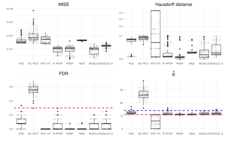
Figure 9: Recovery of the blocks signal in (E3). In each panel, the overall performance over 200 repetitions is summarised as a boxplot and individual repetitions are jittered in dots with a low intensity. In the bottom left panel, the theoretical upper bound $\alpha=0.3$ on the FDR of MUSCLE is marked by a red dashed line. In the bottom right panel, the true numbers of change points in median and in distribution are $K=11$ (marked by a red dashed line) and $K=14$ (marked by a blue dashed line), respectively.

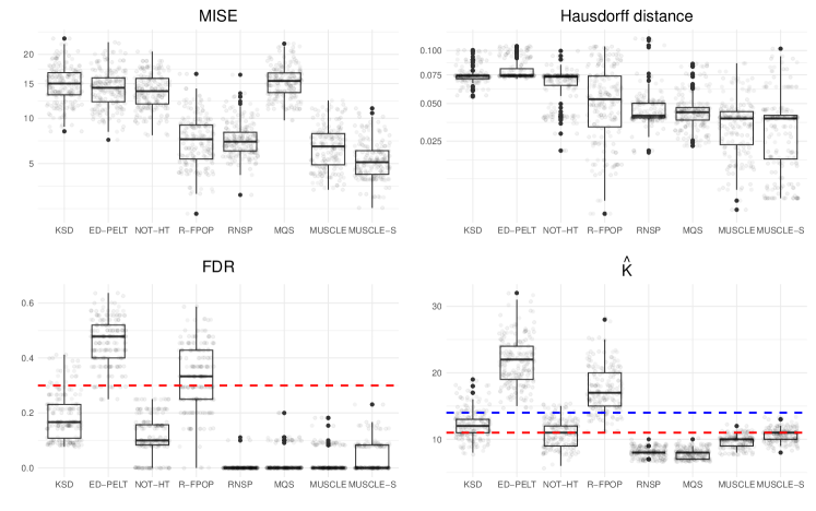
Figure 10: Recovery of the blocks signal in (E4). In each panel, the overall performance over 200 repetitions is summarised as a boxplot and individual repetitions are jittered in dots with a low intensity. In the bottom left panel, the theoretical upper bound $\alpha=0.3$ on the FDR of MUSCLE is marked by a red dashed line. In the bottom right panel, the true numbers of change points in median and in distribution are $K=11$ (marked by a red dashed line) and $K=14$ (marked by a blue dashed line), respectively.

In all scenarios, the simulations are repeated 200 times. We display simulation results in scenarios (E1)–(E2) and (E5) in Figures 3, 4 and 5, respectively. Further detailed results as well as scenarios (E3) and (E4) are given in Appendix B (Figures 9, 10 and 2). In the Gaussian scenario (E1), FDRSeg and WBS overestimate the number of change points, leading to a relatively large FDR. In contrast, PELT, SMUCE and MUSCLE provide more accurate estimation of $K$. Despite MUSCLE having a slightly larger MISE compared to SMUCE and FDRSeg, it outperforms PELT and WBS. Overall, the performance of MUSCLE is comparable to the procedures tailored for the Gaussian model. In non-Gaussian scenarios (E2)–(E5), there are 11 change points in median, and 14 change points in distribution. We compute localisation error, Hausdorff distance, FDR and V-measure with respect to the change points in median, and MISE and MIAE with respect to the median function. We discuss the performance of each method in detail as follows.

• R-FPOP, while being competitive in (E3), exhibits noticeable underperformance in all heteroscedastic scenarios (E2), (E4) and (E5). A possible reason is that R-FPOP estimates the standard deviation of noise using the entire data, which is not well-suited in case of heteroscedasticity.

• NOT-HT performs closely to the best in (E2), but shows an undesirable performance in the other scenarios.

• MQS estimates well the number $K$ of change points in scenarios (E2), (E3) and (E5), while significantly underestimates $K$ in (E4). In all scenarios, the estimated locations of change points are relatively imprecise.

• KSD aims at the detection of distributional changes, but often fails to detect all of $14$ change points. The detected change points contain only a subset of change points in median, as revealed by Hausdorff distance and MISE (as well as localisation error, MIAE and V-measure in Table 2 in Appendix B).

• ED-PELT is also designed to detect changes in distribution. It seriously overestimates the number of change points in all scenarios, and performs even worse than KSD.

• RNSP estimates well the number of change points, and yields competitive median regressions, in scenarios (E2), (E3) and (E5). However, in (E4), it steadily underestimates the number of change points and reports relatively worse Hausdorff distance.

• MUSCLE is among the best ones in all scenarios, and in particular, outperforms the others by a large margin in scenarios (E4) and (E5). The competitive performance of MUSCLE aligns with its statistical guarantees (Section 3). As a speedup variant of MUSCLE, MUSCLE-S has nearly the same performance as MUSCLE, and tends to report slightly more change points.

Regarding computation time, PELT and R-FPOP are the fastest, followed closely by SMUCE, WBS, NOT-HT, MUSCLE-S, MQS and FDRSeg. MUSCLE is noticeably slower, and RNSP and KSD are the slowest. In all considered scenarios, MUSCLE-S is roughly ten times faster than MUSCLE, and takes around 1 s for 2000 samples. See Table 2 in Appendix B.

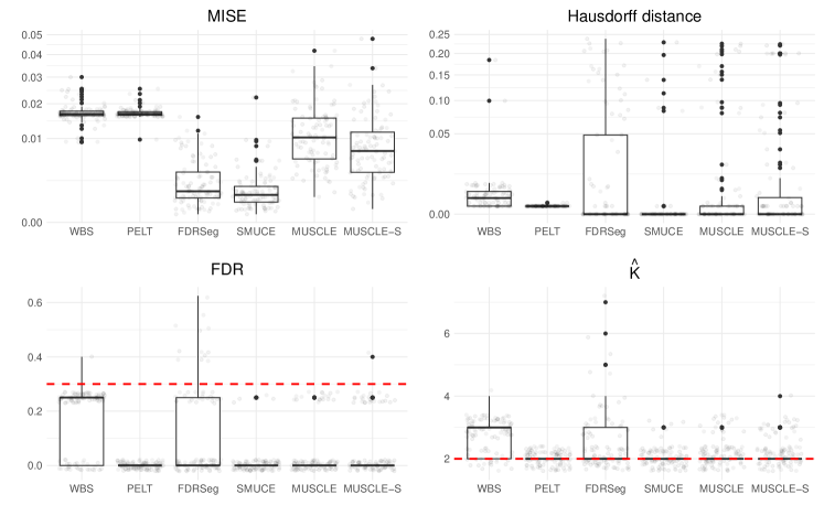
Figure 3: Recovery of the underlying signal in (E1). In each panel, the overall performance over 200 repetitions is summarised as a boxplot and individual repetitions are jittered in dots with a low intensity. In the bottom left panel, the theoretical upper bound $\alpha=0.3$ on the FDR of MUSCLE is marked by a red dashed line. In the bottom right panel, the true number of change points is $K=2$ (marked by a red dashed line).

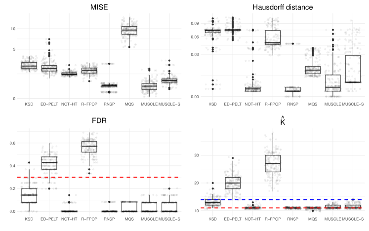
Figure 4: Recovery of the blocks signal in (E2). In each panel, the overall performance over 200 repetitions is summarised as a boxplot and individual repetitions are jittered in dots with a low intensity. In the bottom left panel, the theoretical upper bound $\alpha=0.3$ on the FDR of MUSCLE is marked by a red dashed line. In the bottom right panel, the true numbers of change points in median and in distribution are $K=11$ (marked by a red dashed line) and $K=14$ (marked by a blue dashed line), respectively.

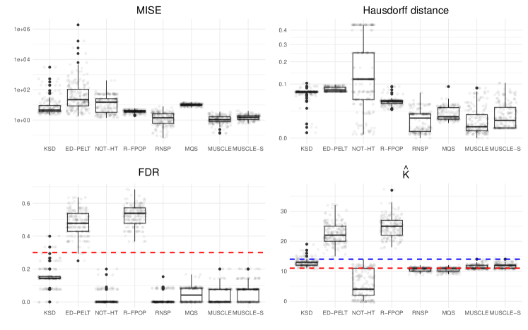
Figure 5: Recovery of the blocks signal in (E5). In each panel, the overall performance over 200 repetitions is summarised as a boxplot and individual repetitions are jittered in dots with a low intensity. In the bottom left panel, the theoretical upper bound $\alpha=0.3$ on the FDR of MUSCLE is marked by a red dashed line. In the bottom right panel, the true numbers of change points in median and in distribution are $K=11$ (marked by a red dashed line) and $K=14$ (marked by a blue dashed line), respectively.

5.1.2 Changes in distribution

We now consider the detection of change points in distribution. If two random variables do not share the same distribution, at least one quantile of them must be different. Thus, a straightforward approach to detect change points in distribution is applying MUSCLE repeatedly to estimate various quantiles of observations, e.g., median ($\beta=0.5$), lower $(\beta=0.25)$ and upper ($\beta=0.75$) quartiles. However, for a change point in distribution, this straightforward approach may report several slightly different estimates when using different quantiles. To address this issue, we modify the multiscale tests on individual segments (see Section 2.1) by considering simultaneously multiple quantiles. Let $\beta=(\beta_{1},\ldots,\beta_{m})\in(0,1)^{m}$ be the considered levels of quantiles. For an interval $I\subseteq[0,\,1)$, we perform a multiscale test on whether $\{Z_{i}:x_{i}\equiv(i-1)/n\in I\}$ have the same $\beta_{r}$-quantile for every $r=1,\ldots,m$. Imitating the development in Section 2, we may arrive at the multiscale side-constraint

$$\mathcal{C}_{k}^{m}\coloneqq\biggl{\{}g=\sum_{j=0}^{k}\theta_{j}\mathbbm{1}_{{I}_{j}}\;:\;\theta_{j}=(\theta_{j1},\ldots,\theta_{jm})\in\mathbb{R}^{m},\,j=0,\ldots,k,\,\bigsqcup_{j=0}^{k}I_{j}=[0,1)\\ \text{ and }\;T_{\accentset{\circ}{I}_{j}}(Z,\theta_{jr})-q_{\alpha/m}(\lvert\accentset{\circ}{I}_{j}\rvert)\leq 0,\,j=0,\dots,k,\,r=1,\ldots,m\biggr{\}}.$$

Note that we use the level $\alpha/m$ in local quantiles $q_{\alpha/m}$ in (4), which comes from the Bonferroni correction on the multiplicity of considering $m$ quantiles. Based on $\mathcal{C}_{k}^{m}$, we introduce a variant of MUSCLE, referred to as M-MUSCLE (Multiple MUSCLE), by

$$\widehat{f}^{m}\;\in\;\underset{f\in\mathcal{C}_{\widehat{K}_{m}}^{m}}{\arg\min}\,\sum_{r=1}^{m}\sum_{i=1}^{n}\bigl{(}Z_{i}-f_{\beta_{r}}(x_{i})\bigr{)}\bigl{(}\beta_{r}-\mathbbm{1}_{\{Z_{i}\leq f_{\beta_{r}}(x_{i})\}}\bigr{)},$$

with $\widehat{K}_{m}\coloneqq\min\bigl{\{}k\in\mathbbm{N}\cup\{0\}\,:\,\mathcal{C}_{k}^{m}\neq\emptyset\bigr{\}}.$ This loss function is also used in composite quantile regression (see e.g. Zou and Yuan, , 2008).

We demonstrate the performance of M-MUSCLE in scenario (E2) with $t_{3}$-noises, see Figure 6. We select $\beta=(\beta_{1},\beta_{2},\beta_{3})=(0.25,0.5,0.75)$ and set $\alpha=0.3$. M-MUSCLE estimates quite accurately the number of change points as well as their locations. In comparison with other nonparametric methods that aim at distributional changes, KSD often underestimates the number of change points, while ED-PELT largely overestimates the number of change points (see Figure 4, the bottom right panel).

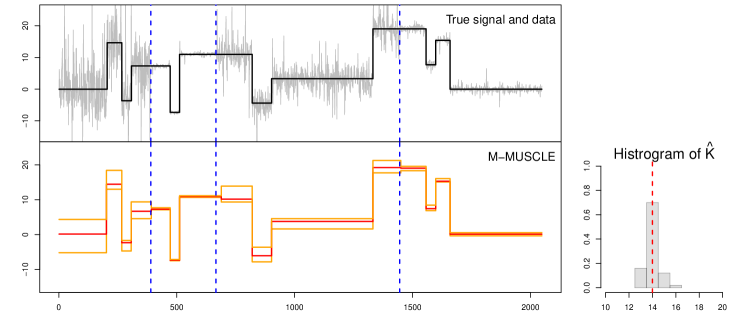
Figure 6: Recovery of the blocks signal in (E2) by M-MUSCLE ($\alpha=0.3$, bottom). The estimated upper and lower quartiles are in orange lines and the estimated median in red line. The histogram on the right summarises its performance in estimating the number of change points over 200 repetitions, where the vertical dashed red line indicates the true number of change points. On the top, the true signal (black line) and the data (grey line) are plotted. Three change points of variances are highlighted by vertical dashed blue lines.

5.2 Real data examples

5.2.1 Well-log dataset

The well-log dataset (Ruanaidh and Fitzgerald, , 2012) contains 4050 measurements of the nuclear magnetic response of underground rocks. Collected by inserting a probe into a borehole, the true signal exhibits approximate piecewise constancy, with each segment corresponding to a distinct rock type characterised by constant physical properties. Change points in the signal reveal changes between rock types, holding crucial importance in the context of oil drilling. We refer to Fearnhead, (2006), Wyse et al., (2011) and Fearnhead and Rigaill, (2019) for further details.

The raw data exhibits several short but sharp oscillations, with some of these fluctuations significantly smaller in amplitude compared to others. Given these distinct patterns, a Gaussian noise assumption might not be justified, which is supported by Shapiro–Wilk’s test, yielding a $p$-value of $2.2\times 10^{-16}$. Consequently, many studies analysing well-log data rely on a pre-cleaned dataset, wherein outliers are manually removed in advance. In general, the detection and removal of outliers are challenging tasks due to the scarcity of labelled data, stemming from the infrequent occurrence of outlier instances. Typical outlier detection methods identify data points that deviate significantly from the rest. However, proposing a universal measure of deviation applicable to all datasets and scenarios is hard or even impossible (cf. Boukerche et al., , 2020).

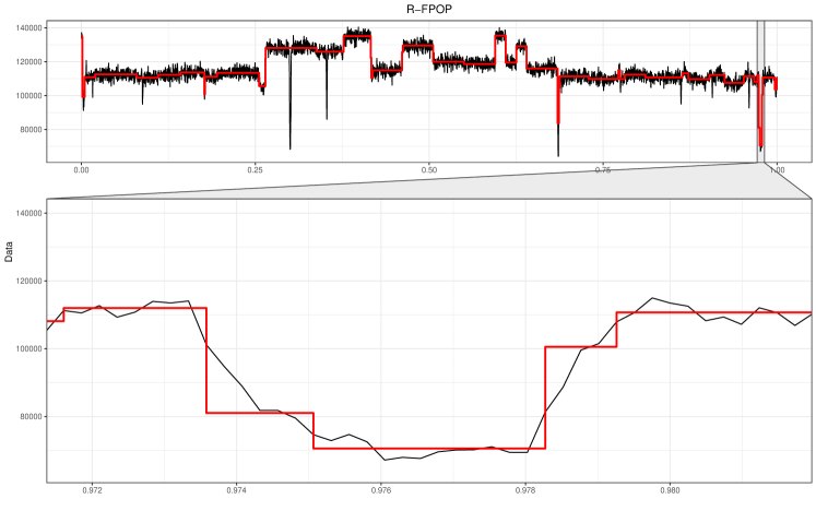
Figure 11: Segmentation of well-log data by R-FPOP. The zoom-in part (around the last flickering event) suggests that R-FPOP overfits the data.

The robustness of MUSCLE eliminates the need for a preliminary pre-cleaning step. We employ MUSCLE to estimate the median ($\beta=1/2$) of well-log signal with different choices of the tuning parameter, namely, $\alpha=0.1,0.3$ and $0.5$, and by comparison we also consider other robust or nonparametric segmentation methods, including KSD, MQS, RNSP, NOT-HT, R-FPOP and ED-PELT, see Figure 7. As shown in the top panel, the raw data has five pronounced flickering events (i.e., events on tiny temporal scales). The estimates provided by KSD, MQS, RNSP and MUSCLE with $\alpha=0.1$ or $0.3$ are very similar, and none of them detect any flickering events. Despite this, they all capture the main shape of the well-log data. We set $\alpha=0.5$ for MQS and RNSP in order to improve their detection power. By contrast, NOT-HT identifies two and R-FPOP detects three flickering events. However, R-FPOP seems to overfit the data around the last flickering (see Figure 11 in Appendix B). ED-PELT reports the highest number of change points. However, as it constantly overestimates $K$ in simulation studies, its estimation may not be trustworthy. With $\alpha=0.5$, MUSCLE successfully recovers all of the five flickering events. In general, it is challenging to verify whether these flickering events (or some of them) are genuine change points or outliers causing by mistakes in measurement. Nevertheless, note that MUSCLE with various choices of $\alpha$ reveals a nested sets of detected features in the well-log data. As a larger $\alpha$ corresponds a lower statistical confidence, such a nested sets of detected features shed light on how likely these features are genuine.

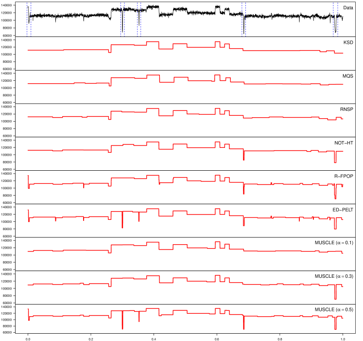
Figure 7: Segmentation of the well-log dataset (Ruanaidh and Fitzgerald, , 2012). The raw data is in the top panel with five pronounced flickering events marked by vertical blue dashed lines. NOT-HT, KSD, R-FPOP and ED-PELT use default parameters. MQS and RNSP are tuned with $\alpha=0.5$.

5.2.2 Ion channels recordings: Gramicidin D

Ion channels are proteins that control ion flows crossing the cell membrane by randomly opening and closing pores and such process is called gating. A popular tool for the quantitative analysis of gating dynamics is the voltage-clamp technique, which allows the measurement of electrical currents flowing through a single ion channel over time (cf. Sakmann, , 2013). Since the measuring process involves an indispensable low-pass filter, the statistical model is

$$Z_{i}=(\rho\ast f)\left(\frac{i}{\omega}\right)+\varepsilon_{i},\quad i=1,\dots,n.$$ (17)

with $\omega$ the sampling rate, and $\rho$ the convolution kernel (corresponding to the low-pass filter). The underlying signal $f$ represents the conductance profile of ion channels, which is a piecewise constant function with change points caused by gating events. The noises $\varepsilon_{i}$ are centred, heterogeneous, and typically non-Gaussian (Venkataramanan et al., , 1998), and they are dependent due to the low-pass filter.

We showcase an extension of MUSCLE to the dependent noises in (17). To take into account the dependence structure, we need to adjust the local quantiles $q_{\alpha}$ in (4). It is generally difficult to determine the dependence of $\mathbbm{1}_{\{{\varepsilon}_{i}\leq 0\}}$, even though the dependence of noises $\varepsilon_{i}$ arises from the known low-pass filter, unless specific assumptions on the noise distribution function are made. Note however that, as a crucial building block of MUSCLE, the multiscale test statistic converges weakly to an accessible distribution in form of supremum of Gaussian random variables under mild conditions (see e.g. Frick et al., , 2014 and Dette et al., , 2020). Inspired by this, we redefine the local quantiles $q_{\alpha}$ in (4) by treating noises $\varepsilon_{i}$ as dependent Gaussian distributed, with the dependence structure derived from the convolution kernel $\rho$. We compute such local quantiles by Monte–Carlo simulations. Another challenge posed by model (17) is that the convoluted signal $\rho*f$ is no longer piecewise constant. But the influence of convolution is only locally active, as the convolution kernel $\rho$ has a compact support. As a consequence, $\rho*f$ is still constant on $[s+\kappa,t)$, with $\kappa$ the kernel length (i.e. the size of the support of $\rho$), if $f$ is constant on $[s,t)$. Thus, we also modify the multiscale statistic $T_{I}$ in (3) by restricting to intervals $J$ such that $J\subseteq I$ and $J-\kappa\subseteq I$. Based on these two adjustments, we obtain an extension of MUSCLE for dependent errors, denoted by D-MUSCLE.

We compare the performance of D-MUSCLE with two state-of-the-art methods JULES (Pein et al., , 2018) and HILDE (Pein et al., , 2020), which are designed especially for ion channel analysis. The implementation of JULES and HILDE is in R package clampSeg on CRAN. We use an ion channel recording of gramicidin D (provided by the Steinem lab, Institute of Organic and Biomolecular Chemistry, University of Göttingen) with the sampling rate $\omega=20$ kHz and the kernel length of 9.6 ms. The results are given in Figure 8. JULES performs relatively worse than the others as it misses a change point at 0.17 s (marked by the vertical dashed line). HILDE, MUSCLE and D-MUSCLE have a close performance, except that MUSCLE and D-MUSCLE report additionally a flickering event between 0.38 s and 0.40 s. Compared with MUSCLE, the detected change points by D-MUSCLE seem more reasonable by visual inspection.

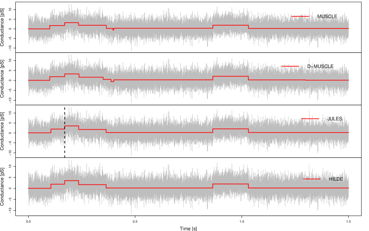
Figure 8: Segmentation of gramicidin D recordings (from the Steinem lab, University of Göttingen). We use the default parameters for JULES (i.e., $\alpha=0.05$) and HILDE (i.e., $\alpha_{1}=0.01,\,\alpha_{2}=0.04$) and tune similarly for the proposed MUSCLE and D-MUSCLE with $\alpha=0.05$. Raw data is in gray lines, and segmentation results are in red lines. In the third panel, a vertical dashed line indicates a missing change point of JULES, which is detected by the other methods.

6 Discussion

In this paper, we introduce a novel change point segmentation method MUSCLE that is robust and meanwhile has a high detection power. It combines the ideas of multiscale testing, quantile segmentation and variational estimation. As a distinctive feature, MUSCLE controls the local errors associated with individual segments. This local error control, as opposed to the commonly studied global error control, allows improved detection power, robustness to data windowing, as well as efficient computation. Under the quantile segmentation model with serial independence, we have established the consistency and the localisation error rates for MUSCLE. Remarkably, these results match (up to log factors) the minimax optimality results in Gaussian setups. Further, we obtain finite sample guarantees on its falsely detected change points in terms of FDR and OER. This provides a statistical interpretation on the unique tuning parameter $\alpha$ of MUSCLE in the sense that the expected proportion of falsely detected change points does not exceed $\alpha$. Moreover, we develop an efficient dynamic programming algorithm for MUSCLE, which leverages advanced wavelet tree data structures, modern pruning techniques, and sparse interval system proposals. We also introduce a speedup variant (denoted by MUSCLE-S) of MUSCLE, which scales linearly with sample size, particularly suitable for large scale datasets. The efficacy of MUSCLE(-S) is validated through comprehensive comparison studies using both simulated and real world data.

We showcase two extensions of MUSCLE and demonstrate their empirical performances. The first extension, denoted as M-MUSCLE, focuses on detecting distributional changes by monitoring multiple quantiles simultaneously. The theoretical properties of MUSCLE would probably extend to M-MUSCLE, and there may be a link to segmentation methods using Wasserstein distances (e.g. Horváth et al., , 2021). The second extension is D-MUSCLE, addressing dependent data. Its statistical guarantees may be derived under the framework of functional dependence (introduced by Wu, , 2005) by additionally requiring the distributions of additive errors to be identical. Further investigation into these extensions, as discussed above, represents intriguing directions for future research.

Finally, the concept of local error appears to be well-suited for online change point detection, as evidenced by its stability across various data windows. Consequently, developing an online version of MUSCLE represents another interesting direction of future research.

7 Acknowledgements

This work was supported by DFG (German Reserach Foundation) CRC 1456 Mathematics of Experiment, and in part by the DFG under Germany’s Excellence Strategy, project EXC 2067 Multiscale Bioimaging: from Molecular Machines to Networks of Excitable Cells (MBExC). The authors thank Manuel Fink and Claudia Steinem (Institute of Organic and Biomolecular Chemistry, University of Göttingen) for providing the ion channel data, and also Axel Munk and Robin Requadt for helpful discussions.

Appendix A Proof of Theorems

A.1 Technical results

Let $W_{1},W_{2},\dots$ are i.i.d. Bernoulli random variables with success probability $\beta$. For any $k,m,i,j\in\mathbb{N}$, $x\in[0,k]$, $1\leq j-i\leq m$, we define

$$A_{k}(x) \coloneqq\frac{x}{k}\log\left(\frac{x}{k}\cdot\frac{1}{\beta}\right)+\left(1-\frac{x}{k}\right)\log\left(\left(1-\frac{x}{k}\right)\cdot\frac{1}{1-\beta}\right),$$

$$B_{m,i,j} \coloneqq\sqrt{2(j-i)A_{j-i}\left(\sum_{k=i}^{j-1}W_{k}\right)}-\sqrt{2\log\left(\frac{em}{j-i}\right)}.$$

Set $\alpha\in(0,1)$ and we consider a series of stopping times:

$$T_{0} \coloneqq 0,$$

$$T_{s} \coloneqq\min\left\{j-1\,\bigg{|}\,\underset{T_{s-1}<i\leq j}{\max}B_{j-T_{s-1},i,j+1}-q_{\alpha}(j-T_{s-1})>0\right\},$$

for $s\geq 1$, where the quantiles $q_{\alpha}(\cdot)$ are given by (4). Furthermore, let

$$S\coloneqq\max\{s\,|\,T_{s}<n\}.$$ (18)

Proposition 7.

Let $S$ be in (18) and $\alpha\in(0,1)$. Then for any $s\in\mathbb{N}$,

$$\mathbb{P}(S\geq s)\leq\alpha^{s}.$$

Moreover, we have

$$\mathbb{E}(S)\leq\frac{\alpha}{1-\alpha}.$$

Proof.

We show that $T_{s}-T_{s-1}$ are i.i.d. distributed for $s\geq 1$:

$$T_{s}-T_{s-1}$$

$$= \min\left\{j-1-T_{s-1}\,\bigg{|}\,\underset{T_{s-1}<i\leq j}{\max}B_{j-T_{s-1},i,j+1}-q_{\alpha}(j-T_{s-1})>0\right\}$$

$$= \min\left\{\tilde{j}-1\,\bigg{|}\,\underset{T_{s-1}<i\leq\tilde{j}+T_{s-1}}{\max}B_{\tilde{j},i,\tilde{j}+T_{s-1}+1}-q_{\alpha}(\tilde{j})>0\right\}$$

$$= \min\left\{\tilde{j}-1\,\bigg{|}\,\underset{0<\tilde{i}\leq\tilde{j}}{\max}B_{\tilde{j},\tilde{i}+T_{s-1},\tilde{j}+T_{s-1}+1}-q_{\alpha}(\tilde{j})>0\right\}$$

$$= \min\Biggl{\{}\tilde{j}-1\,\bigg{|}\,\underset{0<\tilde{i}\leq\tilde{j}}{\max}\sqrt{2(\tilde{j}-\tilde{i}+1)A_{\tilde{j}-\tilde{i}+1}\left(\sum_{k=\tilde{i}}^{\tilde{j}}W_{k+T_{s-1}}\right)}-\sqrt{2\log\left(\frac{e\tilde{j}}{\tilde{j}-\tilde{i}+1}\right)}-q_{\alpha}(\tilde{j})>0\Biggl{\}}$$

with substitutions $\tilde{j}=j-T_{s-1}$ and $\tilde{i}=i-T_{s-1}$. By strong Markov property the sum process $(\sum_{i=1}^{t}W_{i+T})_{t\in\mathbb{N}}$ is independent of $W_{1},\dots,W_{T}$ for any stopping time $T$ condition on $\{T<\infty\}$ (see e.g. Norris, , 1998, Theorem 1.4.2). Thus, $T_{1}-T_{0},T_{2}-T_{1},\dots,T_{s}-T_{s-1},\dots$ are independent. Furthermore, $(\sum_{i=1}^{t}W_{i+T})_{t\in\mathbb{N}}$ is identically distributed for all stopping times, because it is only sum of i.i.d. Bernoulli random variables with parameters $\beta$. This implies that the differences $T_{s}-T_{s-1}$ have the same distribution for all $s\geq 1$. Thus, $T_{1}-T_{0},T_{2}-T_{1},\dots,T_{s}-T_{s-1},\dots$ are i.i.d. random variables. Then

$$\mathbb{P}(S\geq s)\leq\mathbb{P}(T_{s}<n)=\mathbb{P}\left(\sum_{i=1}^{s}T_{i}-T_{i-1}<n\right)\leq\mathbb{P}(T_{1}<n)^{s}.$$

It follows from the definition of $q_{\alpha}(m)$ in (4) that $\mathbb{P}(T_{1}<n)\leq\alpha$ and hence, $\mathbb{P}(S\geq s)\leq\alpha^{s}$. In particular,

$$\mathbb{E}(S)=\sum_{s=1}^{\infty}\mathbb{P}(S\geq s)\leq\sum_{s=1}^{\infty}\alpha^{s}\leq\frac{\alpha}{1-\alpha}.$$

∎

Proposition 8.

Let $\beta\in(0,1)$ and suppose that $Z_{1},\dots,Z_{n}$ have the common $\beta$-quantile, i.e., $f_{\beta}=\theta$ for some $\theta\in\mathbb{R}$. Then for any $k\geq 1$, the estimated number of change point $\widehat{K}$ by MUSCLE satisfies

$$\mathbb{P}\left(\widehat{K}\geq k\right) \leq\alpha^{k},$$ (19)

$$\mathbb{E}\left(\widehat{K}\right) \leq\frac{\alpha}{1-\alpha}.$$ (20)

Proof.

With loss of generality, we assume that $f_{\beta}=0$. Suppose that there exists an estimator $\widetilde{f}=\sum_{k=0}^{\widetilde{K}}\theta_{k}I_{k}$, which has $\widetilde{K}$ change points and satisfies the multiscale side-constrains of $C_{\tilde{K}}$ in (5), then $\widetilde{f}$ has exactly $\widetilde{K}$ false discoveries. Since the MUSCLE minimises the number of estimated change points fulfilling the multiscale side-constrains, we have $\widehat{K}\leq\widetilde{K}$. Therefore, we only need to construct such an estimator $\widetilde{f}$. Let $W_{i}=\mathbbm{1}_{\{Z_{i}\leq 0\}}$ for $i=1,\dots,n$ and

$$\tilde{\theta}=\begin{cases}\min\{Z_{i}\,|\,Z_{i}>0,\,i=1,\dots,n\}/2,&\quad\text{if }\exists\,Z_{i}>0,\\ 1,&\quad\text{otherwise.}\end{cases}$$

Then $\tilde{\theta}>0$. Moreover, by the definition of $\tilde{\theta}$, for any $l\in\mathbb{N}$ the events $\{Z_{i}\leq 0\}$ and $\{Z_{i}\leq\tilde{\theta}/l\}$ are equivalent. Define the stopping time

$$T_{1}=\min\left\{j-1\,|\,T_{[0/n,j/n)}(W,0)>q_{\alpha}(j)\right\}.$$

Set $I_{0}=[0/n,T_{1}/n)$. Then by definition of $T_{1}$ we have $T_{\accentset{\circ}{I_{0}}}(W,0)\leq q_{\alpha}(T_{1})$. We defined the modification $\widetilde{W}_{i}=\mathbbm{1}_{\{Z_{i}\leq\tilde{\theta}\}}$ for all $i/n\in I_{0}$, then $W_{i}=\widetilde{W}_{i}$. Thus,

$$T_{\accentset{\circ}{I_{0}}}(\widetilde{W},\tilde{\theta})=T_{\accentset{\circ}{I_{0}}}(W,0)\leq q_{\alpha}(T_{1}),$$

which indicates that $\tilde{\theta}$ fulfils the multiscale side-constrain on $\accentset{\circ}{I_{0}}$ and therefore, we can estimate $f_{\beta}|_{I_{0}}$ with $\tilde{\theta}$. We continue this procedure until obtain an estimator for whole $f_{\beta}$. More precisely, for any $k\in\mathbb{N}$, let

$$T_{k}=\min\left\{j-1\,|\,T_{[T_{k-1}/n,j/n)}(W,0)>q_{\alpha}(j-T_{k-1})\right\},$$

and $I_{k-1}=[T_{k-1}/n,T_{k}/n)$. The restriction $f_{\beta}|_{I_{k-1}}$ can be estimated by $\tilde{\theta}/k$. Finally, let

$$\widetilde{K}=\max\{k\,|\,T_{k}<n\},$$

and estimation is given by

$$\widetilde{f}=\sum_{k=0}^{\tilde{K}}\tilde{\theta}/(k+1)I_{k}.$$

Since $\tilde{f}$ is piecewise different, it has exactly $\widetilde{K}$ change points. Thus, applying Proposition 7 we have

$$\mathbb{P}\left(\widehat{K}\geq k\right)\leq\mathbb{P}\left(\widetilde{K}\geq k\right)\leq\alpha^{k},$$

and

$$\mathbb{E}\left(\widehat{K}\right)\leq\mathbb{E}\left(\widetilde{K}\right)\leq\frac{\alpha}{1-\alpha}.$$

∎

A.2 Proof of Theorems 1 - 4

Lemma 9.

For any $p,q\in(0,1)$,

$$2(p-q)^{2}\leq p\log\left(\frac{p}{q}\right)+(1-p)\log\left(\frac{1-p}{1-q}\right)\leq\frac{(p-q)^{2}}{q(1-q)}.$$

Proof.

The first inequality follows from Pinsker’s inequality (Tsybakov, , 2009, Lemma 2.5) and (Vanegas et al., , 2022, Theorem A.3). For the second one, we apply the basic inequality $x(x-1)\geq x\log(x)$ for $x>0$, then

$$\frac{p}{q}\log\left(\frac{p}{q}\right) \leq\frac{p}{q}\left(\frac{p}{q}-1\right)$$

$$\frac{1-p}{1-q}\log\left(\frac{1-p}{1-q}\right) \leq\frac{1-p}{1-q}\left(\frac{1-p}{1-q}-1\right)$$

Summing them up gives us the second inequality. ∎

Lemma 10.

Let $\beta\in(0,1)$ be fixed. There exists a constant $C$ such that for all $\alpha\in(0,1)$,

$$\underset{\lvert I\rvert\geq 1}{\sup}\,q_{\alpha}(\lvert I\rvert)\leq C+2\sqrt{2\log\left(\frac{2}{\alpha}\right)},$$

where $q_{\alpha}(\lvert I\rvert)$ is given in (4).

Proof.

Recall from (3) that

$$T_{I}(Z,\theta)\;=\;\underset{J\subseteq{I}}{\max}\sqrt{2L_{J}(Z,\theta)}-\sqrt{2\log\left(\frac{e\lvert I\rvert}{\lvert J\rvert}\right)},$$

where

$$L_{J}(Z,\theta)=\lvert J\rvert\left[\overline{W}_{J}\log\left(\frac{\overline{W}_{J}}{\beta}\right)+(1-\overline{W}_{J})\log\left(\frac{1-\overline{W}_{J}}{1-\beta}\right)\right],$$

$\overline{W}_{J}=\left(\sum_{i\in J}W_{i}\right)/\lvert J\rvert$ and $W_{i}=\mathbbm{1}_{\{Z_{i}\leq\theta\}}\overset{i.i.d.}{\sim}{\rm Ber}(\beta)$ under $H_{I}$. Since $T_{I}(Z,\theta)$ is determined by $W$, in this proof we use $T_{I}(W)$ instead. For any $J\subseteq I$, we define $a_{J}\in\mathbb{R}^{\lvert I\rvert}$ by

$$a_{J,k}=\begin{cases}\frac{1}{\sqrt{\lvert J\rvert}},&\quad\text{if }k\in J,\\ 0,&\quad\text{otherwise},\end{cases}$$

where $a_{J,k}$ denotes the $k$-th component of $a_{J}$. Set $A=\{a_{J}\,|J\subseteq I\}$ and $\lambda_{a}=\sqrt{2\log en\lVert a\rVert_{\infty}^{2}}$. We further define $R_{I}(W)$ and $S_{I}(W)$ by

$$R_{I}(W) =\underset{a\in A}{\max}\sqrt{2}\lvert a^{\top}(W-\beta)\rvert-\lambda_{a}$$

$$S_{I}(W) =\underset{a\in A}{\max}\sqrt{\frac{2}{\beta(1-\beta)}}\lvert a^{\top}(W-\beta)\rvert-\lambda_{a}.$$

Then by Lemma 9 we have

$$R_{I}\leq T_{I}\leq S_{I}.$$

For any $x,y\in\{0,1\}^{\lvert I\rvert}$ and weight $a\in\mathbbm{R}_{\geq 0}^{\lvert I\rvert}$, the weighted Hamming distance $d_{a}$ is given by

$$d_{a}(x,y)=\sum_{i=1}^{\lvert I\rvert}a_{i}\mathbbm{1}_{\{x_{i}\neq y_{i}\}}.$$

We show that $T_{I}$ has the following Lipschitz property for the distance $d_{a}$ with Lipschitz constant $\sqrt{2}$: For any $x\in\{0,1\}^{\lvert I\rvert}$, there exists a $a=a(x)\in\mathbbm{R}_{\geq 0}^{\lvert I\rvert}$ with Euclidean norm $\lVert a\rVert=1$ such that

$$T_{I}(x)-T_{I}(y)\leq Ld_{a}(x,y),\quad\forall y\in\{0,1\}^{\lvert I\rvert}.$$

For any $x,y\in\{0,1\}^{\lvert I\rvert}$, let $\tilde{a}=\tilde{a}(x)$ denote the maximizer of $S_{I}(x)$

$$\,T_{I}(x)-T_{I}(y)$$

$$\leq \,S_{I}(x)-R_{I}(y)$$

$$= \,\underset{a\in A}{\max}\left(\sqrt{\frac{2}{\beta(1-\beta)}}\lvert a^{\top}(x-\beta)\rvert-\lambda_{a}\right)-\underset{a\in A}{\max}\left(\sqrt{2}\lvert a^{\top}(y-\beta)\rvert-\lambda_{a}\right)$$

$$= \,\sqrt{\frac{2}{\beta(1-\beta)}}\lvert\tilde{a}^{\top}(x-\beta)\rvert-\lambda_{\tilde{a}}-\underset{a\in A}{\max}\left(\sqrt{2}\lvert\tilde{a}^{\top}(y-\beta)\rvert-\lambda_{a}\right)$$

$$\leq \,\sqrt{2}\lvert\tilde{a}^{\top}(x-\beta)\rvert-\lambda_{\tilde{a}}-\sqrt{2}\lvert\tilde{a}^{\top}(y-\beta)\rvert+\lambda_{\tilde{a}}$$

$$= \,\sqrt{2}\lvert\tilde{a}^{\top}(x-\beta)\rvert-\sqrt{2}\lvert\tilde{a}^{\top}(y-\beta)\rvert$$

$$\leq \,\sqrt{2}\lvert\tilde{a}^{\top}(x-y)\rvert=\sqrt{2}\sum_{i=1}^{\lvert I\rvert}\tilde{a}_{i}\mathbbm{1}_{\{x_{i}\neq y_{i}\}}=\sqrt{2}d_{\tilde{a}}(x,y),$$

where the second last equality follows the fact $x,y\in\{0,1\}^{\lvert I\rvert}$. Let $M_{I}$ denote the median of $T_{I}$. By Frick et al., (2014); Dümbgen and Spokoiny, (2001); Dümbgen et al., (2006) the random sequence $T_{I}$ converges in distribution a almost surely finite random variable $M$ as $\lvert I\rvert\to\infty$, thus median of $M$ is finite and $C\coloneqq\sup_{\lvert I\rvert\in\mathbb{N}}M_{I}<\infty$. Applying (Giné and Nickl, , 2016, Corollary 3.2.5) we have for any $t>0$

$$\mathbb{P}(T_{I}-M_{I}\geq t)\leq 2\exp{\left(-t^{2}/8\right)}.$$

By choosing $t=2\sqrt{2\log(2/\alpha)}$ we have for any $\lvert I\rvert\in\mathbb{N}$

$$q_{\alpha}(\lvert I\rvert)\leq M_{I}+2\sqrt{2\log\left(\frac{2}{\alpha}\right)}\leq C+2\sqrt{2\log\left(\frac{2}{\alpha}\right)}.$$

∎

Proof of Theorem 1.

Recall from Section 3.1 that

$$I_{k}=\left(\tau_{k}-\frac{\lambda_{k}}{2},\tau_{k}+\frac{\lambda_{k}}{2}\right),$$

where $\lambda_{k}=\min\{\tau_{k}-\tau_{k-1},\tau_{k+1}-\tau_{k}\}$. By definition, these intervals are disjoint. Let $\theta_{k}^{+}=\max\{\theta_{k-1},\theta_{k}\}$ and $\theta_{k}^{-}=\min\{\theta_{k-1},\theta_{k}\}$ and spilt $I_{k}$ accordingly, i.e.,

$$I_{k}^{+}=\{t\in I_{k}\,|\,f(t)=\theta_{k}^{+}\},\text{ and }I_{k}^{-}=\{t\in I_{k}\,|\,f(t)=\theta_{k}^{-}\}.$$

Assume that $\widehat{K}<K$ and let $\widehat{I}_{0},\dots,\widehat{I}_{\widehat{K}}$ denote the estimated segments. Since $\widehat{K}<K$, there exists a interval $I_{k}$ such that $I_{k}$ is completely contained in some estimated segment, say $\widehat{I}_{*}$. This can be verified by contradiction: Suppose that there is no such interval, then any interval $I_{k}$ contains at least one estimated change point. Since $I_{k}$’s are disjoint, then we have $\widehat{K}\geq K$, which contradicts to the underestimation assumption. Thus, there exists a $I_{k}$ is contained in some estimated segment $\widehat{I}_{*}$, i.e., no change point is detected on $I_{k}$.

We show that the probability that no change point can be detected on $I_{k}$ is sufficiently small. To this end, we consider the event that there exists a constant on $\widehat{I}_{*}$ fulfilling the multiscale side-constrains on both $I_{k}^{+}$ and $I_{k}^{-}$. Define

$$C_{k}=\Bigg{\{}\exists c\in\mathbb{R}\Bigg{|}\sqrt{2L_{I_{k}^{+}}(Z,c)}-\sqrt{2\log\left(\frac{e\lvert\widehat{I}_{*}\rvert}{\lvert I_{k}^{+}\rvert}\right)}\leq q_{\alpha}(\lvert\widehat{I}_{*}\rvert)\text{ and }\sqrt{2L_{I_{k}^{-}}(Z,c)}-\sqrt{2\log\left(\frac{e\lvert\widehat{I}_{*}\rvert}{\lvert I_{k}^{-}\rvert}\right)} \leq q_{\alpha}(\lvert\widehat{I}_{*}\rvert)\Bigg{\}}$$

Note that either $c\geq\theta_{k}^{+}-\delta_{k}/2$ or $c\geq\theta_{k}^{-}+\delta_{k}/2$, we define

$$C_{k}^{+} =\left\{\exists c\geq\theta_{k}^{+}-\frac{\delta_{k}}{2}\bigg{|}\sqrt{2L_{I_{k}^{+}}(Z,c)}-\sqrt{2\log\left(\frac{e\lvert\widehat{I}_{*}\rvert}{\lvert I_{k}^{+}\rvert}\right)}\leq q_{\alpha}(\lvert\widehat{I}_{*}\rvert)\right\},$$

$$C_{k}^{-} =\left\{\exists c\leq\theta_{k}^{-}+\frac{\delta_{k}}{2}\bigg{|}\sqrt{2L_{I_{k}^{-}}(Z,c)}-\sqrt{2\log\left(\frac{e\lvert\widehat{I}_{*}\rvert}{\lvert I_{k}^{-}\rvert}\right)}\leq q_{\alpha}(\lvert\widehat{I}_{*}\rvert)\right\}.$$

Obviously, we have $C_{k}\subseteq C_{k}^{+}\cup C_{k}^{-}$. Note that $C_{k}^{+}$ and $C_{k}^{-}$ are independent. We obtain

$$\mathbb{P}(C_{k})\leq 1-(1-\mathbb{P}(C_{k}^{+}))(1-\mathbb{P}(C_{k}^{-})).$$

We provide an upper bound of $\mathbb{P}(C_{k}^{-})$, then the probability $\mathbb{P}(C_{k}^{+})$ can be upper bounded in a similar way. For any $i\in I_{k}^{-}$, we have $F_{i}^{-1}(\beta)=\theta_{k}^{-}$. Further set $F^{-}_{\min,k}=\min_{i\in I_{k}^{-}}F_{i}$ and $\bar{F}_{k}^{-}=\left(\sum_{i\in I_{k}^{-}}F_{i}\right)/\lvert I_{k}^{-}\rvert$. Let

$$\zeta_{I_{k}^{-}}=\inf\left\{x\in\mathbb{R}\Bigg{|}\sum_{i\in I_{k}^{-}}\mathbbm{1}_{\{Z_{i}\leq x\}}\geq\lvert I_{s}^{-}\rvert\beta\right\}$$

be the empirical quantile of the observations on $I_{k}^{-}$. For all $c\geq\theta_{k}^{-}+\delta_{k}/2$, if $\zeta_{I_{k}^{-}}\leq\theta_{k}^{-}+\delta_{k}/2$, then

$$\beta\leq\overline{W}(Z,\zeta_{I_{k}^{-}})\leq\overline{W}\left(Z,\theta_{k}^{-}+\frac{\delta}{2}\right)\leq\overline{W}(Z,c),$$ (21)

where $\overline{W}(Z,x)=\sum_{i\in I_{k}^{-}}\mathbbm{1}_{\{Z_{i}\leq x\}}/\lvert I_{k}^{-}\rvert$. Note that the function

$$g:x\mapsto\lvert I_{k}^{-}\rvert\left(x\log\left(\frac{x}{\beta}\right)+(1-x)\log\left(\frac{1-x}{1-\beta}\right)\right)$$

is strictly convex with minimum $g(\beta)=0$, hence $g$ is strictly increasing on $(\beta,1)$. Thus, by (21)

$$L_{I_{k}^{-}}(Z,c)=g\left(\overline{W}(Z,c)\right)\geq g\left(\overline{W}\left(Z,\theta_{k}^{-}+\frac{\delta_{k}}{2}\right)\right)=L_{I_{k}^{-}}\left(Z,\theta_{k}^{-}+\frac{\delta_{k}}{2}\right).$$

Therefore,

$$\mathbb{P}(C_{k}^{-})\leq \,\mathbb{P}\left(C_{k}^{-}\cap\left\{\zeta_{I_{k}^{-}}\leq\theta_{k}^{-}+\frac{\delta_{k}}{2}\right\}\right)+\mathbb{P}\left(\zeta_{I_{k}^{-}}>\theta_{k}^{-}+\frac{\delta_{k}}{2}\right)$$

$$\leq \,\mathbb{P}\left(\sqrt{2L_{I_{k}^{-}}\left(Z,\theta_{k}^{-}+\frac{\delta_{k}}{2}\right)}-\sqrt{2\log\left(\frac{e\lvert\widehat{I}_{*}\rvert}{\lvert I_{k}^{-}\rvert}\right)}\leq q_{\alpha}(\lvert\widehat{I}_{*}\rvert)\right)+\mathbb{P}\left(\zeta_{I_{k}^{-}}>\theta_{k}^{-}+\frac{\delta_{k}}{2}\right)$$

$$\leq \,\mathbb{P}\left(L_{I_{k}^{-}}\left(Z,\theta_{k}^{-}+\frac{\delta_{k}}{2}\right)\leq\frac{\left(q_{\alpha}(\lvert\widehat{I}_{*}\rvert)+\sqrt{2\log\left(\frac{e\lvert\widehat{I}_{*}\rvert}{\lvert I_{k}^{-}\rvert}\right)}\right)^{2}}{2}\right)+\mathbb{P}\left(\zeta_{I_{k}^{-}}>\theta_{k}^{-}+\frac{\delta_{k}}{2}\right)$$

$$\leq \,2\exp\left(-\frac{\left(\sqrt{2n\lambda_{k}}\xi_{\bar{F}^{-}_{\beta}}(\delta_{k}/2)-q_{\alpha}(\lvert\widehat{I}_{*}\rvert)-\sqrt{2\log\left(\frac{e\lvert\widehat{I}_{*}\rvert}{\lvert I_{k}^{-}\rvert}\right)}\right)^{2}_{+}}{2}\right)+2\exp\left(-n\lambda_{k}\xi_{F^{-}_{\min,\beta}}(\delta_{k}/2)^{2}\right),$$

where the last two inequalities follow from (Vanegas et al., , 2022, Theorem A.2 and A.3), respectively. Note that the facts $\xi_{k}\leq\xi_{F^{-}_{\min,k},\beta}(\delta_{k}/2)\leq\xi_{\bar{F}_{k}^{-},{\beta}}(\delta_{k}/2)$, $q_{\alpha}(\lvert\widehat{I}_{*}\rvert)\leq\max_{m\leq n}q_{\alpha}(m)$ and $\lvert\widehat{I}_{*}\rvert\leq n$ we have

$$\mathbb{P}(C_{k})\leq 1-(1-\mathbb{P}(C_{k}^{+}))(1-\mathbb{P}(C_{k}^{-}))\leq 1-\gamma_{n,k}^{2},$$

where $\gamma_{n,k}$ is given by

$$\gamma_{n,k}=1-2\exp{\left(-n\lambda_{k}\xi_{k}^{2}\right)}-2\exp{\left(-\left(\sqrt{n\lambda_{k}}\xi_{k}-\frac{1}{\sqrt{2}}\underset{m\leq n}{\max}q_{\alpha}(m)-\sqrt{\log\frac{2e}{\lambda_{k}}}\right)_{+}^{2}\right)}.$$

Note that if all of these $K$ change-points are detected, then $\widehat{K}\geq K$, i.e.,

$$\mathbb{P}(\widehat{K}\geq K)\geq\mathbb{P}\left(\cap_{k=1}^{K}C_{k}^{c}\right)=\prod_{k=1}^{K}(1-\mathbb{P}(C_{k}))\geq\prod_{k=1}^{K}\gamma_{n,k}^{2},$$

which proves the first claim. By the definitions of $\Lambda$ and $\Omega$ in (8) we have for all $k=1,\dots,K$,

$$\gamma_{n,k}^{2}\geq\Bigg{(}1-2\exp\left(-\left(\sqrt{n}\Omega-\frac{1}{\sqrt{2}}\underset{m\leq n}{\max}q_{\alpha}(m)-\sqrt{\log\left(\frac{2e}{\Lambda}\right)}\right)_{+}^{2}\right)-2\exp\left(-n\Omega^{2}\right)\bigg{)}^{2}\eqqcolon\gamma_{n}.$$

Thus, applying Bernoulli’s inequality we have

$$\mathbb{P}(\widehat{K}<K)\leq 1-\gamma_{n}^{K}\leq 4K\Bigg{(}\exp\left(-\left(\sqrt{n}\Omega-\frac{1}{\sqrt{2}}\underset{m\leq n}{\max}q_{\alpha}(m)-\sqrt{\log\left(\frac{2e}{\Lambda}\right)}\right)_{+}^{2}\right)+\exp\left(-n\Omega^{2}\right)\Bigg{)}.$$

∎

Proof of Theorem 2.

Let $T(f)$ denote the set of all change points of $f$. Note that

$$\,\mathbb{P}(\widehat{K}\geq K+k)$$

$$\leq \,\mathbb{P}\left(\max\,T_{I_{i}}(Z,\widehat{\theta}_{i})-q_{\alpha}(\lvert I_{i}\rvert)\geq 0,\forall\widehat{f}\in\Sigma\text{ with }\lvert T(\widehat{f})\rvert\leq K+k-1\right)$$

$$\leq \,\mathbb{P}\left(\max\,T_{I_{i}}(Z,\widehat{\theta}_{i})-q_{\alpha}(\lvert I_{i}\rvert)\geq 0,\forall\widehat{f}\in\Sigma\text{ with }T(f)\subseteq T(\widehat{f})\text{ and }\lvert T(\widehat{f})\rvert\leq K+k-1\right)$$

$$\leq \,\mathbb{P}\left(\max T_{I_{i}}(Z-f,\widehat{\theta}_{i}-f|_{I_{i}})-q_{\alpha}(\lvert I_{i}\rvert)\geq 0,\forall\widehat{f}\in\Sigma\text{ with }\lvert T(\widehat{f}-f)\rvert\leq k-1\right).$$

Let $\widetilde{Z}=Z-f$, then each $\widetilde{Z}_{i}$ has $\beta$-quantile zero. The event in last lines implies that the estimator for zero function supplied by MUSCLE has at least $k$ change points. Thus, it follows from Proposition 8 that

$$\mathbb{P}(\widehat{K}\geq K+k)\leq\mathbb{P}(T_{k}<n)\leq\alpha^{k}.$$

∎

Proof of Theorem 3.

It follows from Theorems 1 and 2 that

$$\mathbb{P}(\widehat{K}_{n}\neq K_{n})\leq \,4K_{n}\Bigg{(}\exp\left(-\left(\sqrt{n}\Omega_{n}-\frac{1}{\sqrt{2}}\underset{m\leq n}{\max}q_{\alpha}(n)-\sqrt{\log\left(\frac{2e}{\Lambda_{n}}\right)}\right)_{+}^{2}\right)+\exp\left(-n\Omega_{n}^{2}\right)\Bigg{)}+\alpha_{n}$$

$$= \,4\exp{(-\Gamma_{1,n})}+4\exp{(-\Gamma_{2,n})}+\alpha_{n},$$

where

$$\Gamma_{1,n} =\left(\sqrt{n}\Omega_{n}-\frac{1}{\sqrt{2}}\underset{m\leq n}{\max}q_{\alpha}(n)-\sqrt{\log\left(\frac{2e}{\Lambda_{n}}\right)}\right)_{+}^{2}-\log K_{n},$$

$$\Gamma_{2,n} =n\Omega_{n}^{2}-\log K_{n}.$$

Note that $\Gamma_{1,n}\leq\Gamma_{2,n}$ for all large $n$ and $\alpha_{n}\to 0$, it is sufficient to show that $\Gamma_{1,n}\to\infty$ as $n\to\infty$. In the first case: $\liminf\Lambda_{n}>0$ implies that both $\sqrt{\log(2e/\Lambda_{n})}$ and $K_{n}$ are finite, thus the condition

$$\sqrt{n}\Omega_{n}-\frac{1}{\sqrt{2}}\underset{m\leq n}{\max}q_{\alpha}(n)\to\infty,$$

ensures that $\Gamma_{1,n}\to\infty$.

For the second case: Note that $K_{n}\leq\Lambda_{n}^{-1}$ and $\sqrt{n}\Omega_{n}\geq c\sqrt{-\log\Lambda_{n}}$ for some $c>2$ and apply the basic inequality $\sqrt{x+y}-\sqrt{x}\geq y/(2\sqrt{x})$ for all $x,y\geq 0$, we then have

$$\Gamma_{1,n} \geq\left(c\sqrt{-\log\Lambda_{n}}-\frac{1}{\sqrt{2}}\underset{m\leq n}{\max}q_{\alpha}(n)-\sqrt{\log\left(\frac{2e}{\Lambda_{n}}\right)}\right)_{+}^{2}-\left(\sqrt{-\log\Lambda_{n}}\right)^{2}.$$

$$\geq\left((c-1)\sqrt{-\log\Lambda_{n}}-\frac{1}{\sqrt{2}}\underset{m\leq n}{\max}q_{\alpha}(n)-\frac{\log 2e}{2\sqrt{-\log\Lambda_{n}}}\right)_{+}^{2}-\left(\sqrt{-\log\Lambda_{n}}\right)^{2}$$

$$\geq\left((c-2)\sqrt{-\log\Lambda_{n}}-\frac{1}{\sqrt{2}}\underset{m\leq n}{\max}q_{\alpha}(n)-\frac{\log 2e}{2\sqrt{-\log\Lambda_{n}}}\right)_{+}^{2}\to\infty,$$

where the last inequality comes from another basic inequality $(x+y)^{2}-x^{2}\geq y^{2}$ for all $x,y\geq 0$. ∎

Proof of Theorem 4.

We consider the probability of $d_{H}(T_{n},\widehat{T}_{n})\geq\varepsilon_{n}$. Obviously,

$$\mathbb{P}\left(d_{H}(T_{n},\widehat{T}_{n})\geq\varepsilon_{n}\right)\leq\mathbb{P}\left(\max_{k}\min_{j}\lvert\tau_{k}-\widehat{\tau}_{j}\rvert\geq\varepsilon_{n}\right)+\mathbb{P}\left(\max_{k}\min_{j}\lvert\tau_{k}-\widehat{\tau}_{j}\rvert<\varepsilon_{n},\max_{j}\min_{k}\lvert\tau_{k}-\widehat{\tau}_{j}\rvert\geq\varepsilon_{n}\right).$$ (22)

We bound both probabilities in (22) from above separately.

For the first probability: If $\max_{k}\min_{j}\lvert\tau_{k}-\widehat{\tau}_{j}\rvert\geq\varepsilon_{n}$, then there exists $k\in\{1,\dots,K_{n}\}$ such that on $I_{k}=(\tau_{k}-\varepsilon_{n},\tau_{k}+\varepsilon_{n})$ no change point is detected. Since $2\varepsilon_{n}\leq\Lambda_{n}$, the interval $I_{k}\subseteq(\tau_{k}-\Lambda_{n}/2,\tau_{k}+\Lambda_{n}/2)$. Applying the same technique as in the proof of Theorem 1 and replacing $\Lambda_{n}$ by $\varepsilon_{n}$ we obtain the first upper bound.

Next we study the second probability: We decompose $\widehat{T}_{n}$ into two disjoint sets $A_{n}$ and $B_{n}$, where

$$A_{n} =\{\widehat{\tau}\in\widehat{T}_{n}:\min_{k}\lvert\widehat{\tau}-\tau_{k}\rvert<\varepsilon_{n}\},$$

$$B_{n} =\{\widehat{\tau}\in\widehat{T}_{n}:\min_{k}\lvert\widehat{\tau}-\tau_{k}\rvert\geq\varepsilon_{n}\}.$$

Since $\max_{k}\min_{j}\lvert\tau_{k}-\widehat{\tau}_{j}\rvert<\varepsilon_{n}$, we have for any true change point $\tau_{k}$, there exists an estimated change point $\widehat{\tau}_{j(k)}$ such that $\lvert\tau_{k}-\widehat{\tau}_{j}\rvert<\varepsilon_{n}$, that is, $\widehat{\tau}_{j(k)}\in I_{k}$ for all $k=1,\dots,K_{n}$. Note that $I_{k}$’s are pairwise disjoint, thus $\widehat{\tau}_{j(k)}$’s are pairwise distinct. By definition, all $\widehat{\tau}_{j(k)}$’s belong to $A_{n}$ and therefore $\lvert A_{n}\rvert\geq K$. Furthermore, the event $\max_{j}\min_{k}\lvert\tau_{k}-\widehat{\tau}_{j}\rvert\geq\varepsilon_{n}$ implies that there exists a $j^{*}$ such that $\lvert\tau_{k}-\widehat{\tau}_{j^{*}}\rvert\geq\varepsilon_{n}$ for all $k=1,\dots,K_{n}$, i.e., $\widehat{\tau}_{j^{*}}\in B_{n}$ and $\lvert B_{n}\rvert\geq 1$. Since $\widehat{T}_{n}=A_{n}\dot{\sqcup}B_{n}$, we have $\lvert\widehat{T}_{n}\rvert\geq K_{n}+1$. Therefore, by Theorem 2 the second probability is upper bounded by $\mathbb{P}(\widehat{K}_{n}\geq K_{n}+1)\leq\alpha_{n}$. This finishes the proof. ∎

A.3 Proof of Theorem 5

Let $\alpha\in(0,1)$. We first construct an upper bound for expectation of the number of false discoveries (denoted by $\rm{FD}(\alpha)$) given there is no true discovery.

Lemma 11.

Under above notations we have

$$\mathbb{E}(\rm{FD}(\alpha)|TD(\alpha)=0)\leq\frac{\alpha}{1-\alpha}\eqqcolon G(\alpha)$$

Proof.

Note that it is sufficient to prove the claim for constant signal and we may assume that it equals to zero. We study the estimator $\widetilde{f}$ with $\widetilde{K}$ change points, which is defined in the proof of Proposition 8. Again, since MUSCLE minimises the number of estimated change points, the FD of MUSCLE is upper bounded by $\widetilde{K}$. Thus, apply Proposition 8 we have

$$\mathbb{E}({\rm FD(\alpha)}|{\rm TD}(\alpha)=0)\leq\mathbb{E}(\widetilde{K})\leq\frac{\alpha}{1-\alpha}\eqqcolon G(\alpha).$$

∎

Proof of Theorem 5.

Applying Lemma 11, Li et al., (2016, Lemma A.2) and the technique in Li et al., (2016, proof of Theorem 2.2) we have

$${\rm FDR}\leq\frac{G(\alpha)}{1+G(\alpha)}=\alpha.$$

Next we prove the statement on OER. It follows from Theorem 2 that $\mathbb{P}(\widehat{K}-K\geq k)\leq\alpha^{k}$. Thus,

$$\mathbb{E}((\widehat{K}-K)_{+})=\sum_{k=1}^{\infty}\mathbb{P}(\widehat{K}-K\geq k)\leq\frac{\alpha}{1-\alpha}.$$

If $K=0$, then

$$\mathbb{E}\left(\frac{(\widehat{K}-K)_{+}}{\widehat{K}\vee 1}\right)=\mathbb{E}\left(\frac{\widehat{K}}{\widehat{K}}\mathbbm{1}_{\{\widehat{K}\geq 1\}}\right)=\mathbb{P}(\widehat{K}\geq 1)\leq\alpha.$$

For $K\geq 1$,

$$\frac{(\widehat{K}-K)_{+}}{\widehat{K}\vee 1}=\frac{(\widehat{K}-K)_{+}}{(\widehat{K}-K)_{+}+K}.$$

Note that the function $x\mapsto x/(x+K)$ is strictly concave and monotone increasing on $[1,\infty)$. By Jensen’s inequality we have

$$\mathbb{E}\left(\frac{(\widehat{K}-K)_{+}}{\widehat{K}+1}\right)\leq \frac{\mathbb{E}((\widehat{K}-K)_{+})}{\mathbb{E}((\widehat{K}-K)_{+})+K}$$

$$\leq \frac{\frac{\alpha}{1-\alpha}}{\frac{\alpha}{1-\alpha}+K}=\frac{\alpha}{(1-\alpha)K+\alpha}.$$

∎

Appendix B Additional materials of simulation study

Suppose that $Z_{1},\dots,Z_{n}$ are observations from Model 1 with underlying signal $f_{\beta}$. Let $\widehat{f}$ denote an estimate of $f_{\beta}$. Then the mean integrated squared error (MISE) of $\widehat{f}$ is given by

$${\rm MISE}\left(\widehat{f}\right)=\frac{1}{n}\sum_{i=1}^{n}\left(\widehat{f}(x_{i})-f_{\beta}(x_{i})\right)^{2}.$$ (23)

Furthermore, we define the mean integrated absolute error (MIAE) of $\widehat{f}$ by

$${\rm MIAE}\left(\widehat{f}\right)=\frac{1}{n}\sum_{i=1}^{n}\left|\widehat{f}(x_{i})-f_{\beta}(x_{i})\right|.$$ (24)

For RNSP, MQS and MUSCLE we apply empirical quantiles to fit data on each segments and for other procedures we use sample means instead.

Table 2: Statistical performance of procures mentioned in Section 5.1.1 in Gaussian (E1), scaled $t_{3}$ (E2), scaled Cauchy (E3), scaled centred $\chi_{3}^{2}$-distribution (E4) and mixed distribution (E5). Medians of each quantity and their mean absolute deviations (in brackets) are presented. For each quantity, the best performances are highlighted in bold.

Scenarios	Methods	MISE	MIAE	$L(T;\widehat{T})$	$d_{H}(T,\widehat{T})$	$\widehat{K}$	FDR	V-meas.	Time
(E1)	MUSCLE	$0.010$	$0.074$	$\mathbf{0}$	$\mathbf{0}$	$\mathbf{2}$	$\mathbf{0}$	$\mathbf{1}$	$15.871$
		($0.006$)	($0.001$)	($0.0002$)	($0.0350$)	($0.29$)	($0.07$)	($0.036$)	($3.344$)
	MUSCLE-S	$0.007$	$0.051$	$\mathbf{0}$	$\mathbf{0}$	$\mathbf{2}$	$\mathbf{0}$	$\mathbf{1}$	$0.697$
		($0.005$)	($0.024$)	($0.0002$)	($0.0442$)	($0.38$)	($0.09$)	($0.047$)	($0.309$)
	SMUCE	$\mathbf{0.001}$	$\mathbf{0.025}$	$\mathbf{0}$	$\mathbf{0}$	$\mathbf{2}$	$\mathbf{0}$	$\mathbf{1}$	$0.026$
		$(0.001)$	$(0.010)$	$(4.8\cdot 10^{-5})$	$(0.0159)$	$(0.11)$	$(0.03)$	$(0.017)$	$(0.002)$
	FDRSeg	$\mathbf{0.001}$	$0.027$	$\mathbf{0}$	$\mathbf{0}$	$\mathbf{2}$	$\mathbf{0}$	$\mathbf{1}$	$1.068$
		$(0.002)$	$(0.010)$	$(5.6\cdot 10^{-5})$	$(0.0542)$	$(0.71)$	$(0.15)$	$(0.065)$	$(1.689)$
	WBS	$0.017$	$0.032$	$5\cdot 10^{-4}$	$0.0002$	$3$	$0.25$	$0.988$	$0.076$
		$(0.001)$	$(0.009)$	$(7.4\cdot 10^{-4})$	$(0.0058)$	$(0.41)$	$(0.10)$	$(0.006)$	$(0.004)$
	PELT	$0.017$	$0.029$	$5\cdot 10^{-4}$	$5\cdot 10^{-4}$	$\mathbf{2}$	$\mathbf{0}$	$0.999$	$\mathbf{7\cdot 10^{-4}}$
		$(0.001)$	$(0.009)$	$(1.9\cdot 10^{-4})$	$(1.9\cdot 10^{-4})$	$(0)$	$(0)$	$(0.001)$	$(9.9\cdot 10^{-5})$
(E2)	MUSCLE	$\mathbf{0.315}$	$0.188$	$0.0009$	$0.0014$	$\mathbf{11}$	$\mathbf{0}$	$\mathbf{0.996}$	$6.278$
		$(0.225)$	$(0.042)$	$(0.0010)$	$(0.0100)$	$(0.46)$	$(0.03)$	$(0.005)$	$(0.583)$
	MUSCLE-S	$0.665$	$0.232$	$0.0034$	$0.0034$	$\mathbf{11}$	$\mathbf{0}$	$0.990$	$0.715$
		$(0.221)$	$(0.043)$	$(0.0004)$	$(0.0197)$	$(0.67)$	$(0.04)$	$(0.010)$	$(0.142)$
	MQS	$9.611$	$0.900$	$0.0112$	$0.0117$	$\mathbf{11}$	$\mathbf{0}$	$0.923$	$0.874$
		$(1.277)$	$(0.105)$	$(0.0021)$	$(0.0077)$	$(0.20)$	$(0.04)$	$(0.008)$	$(0.036)$
	NOT-HT	$1.219$	$0.306$	$0.0009$	$0.0009$	$\mathbf{11}$	$\mathbf{0}$	$0.985$	$0.180$
		$(0.148)$	$(0.048)$	$(0.0010)$	$(0.0080)$	$(0.16)$	$(0.01)$	$(0.003)$	$(0.009)$
	KSD	$2.167$	$0.438$	$0.0029$	$0.0732$	$13$	$0.14$	$0.942$	$70.411$
		$(0.469)$	$(0.072)$	$(0.0031)$	$(0.0115)$	$(0.97)$	$(0.05)$	$(0.015)$	$(5.274)$
	R-FPOP	$1.632$	$0.495$	$0.0009$	$0.0488$	$27$	$0.57$	$0.902$	$\mathbf{0.002}$
		$(0.330)$	$(0.066)$	$(0.0007)$	$(0.0168)$	$(3.44)$	$(0.06)$	$(0.020)$	$(2\cdot 10^{-4})$
	ED-PELT	$1.838$	$0.406$	$0.0009$	$0.0747$	$20$	$0.43$	$0.905$	$0.118$
		$(0.544)$	$(0.066)$	$(0.0007)$	$(0.0037)$	$(2.20)$	$(0.06)$	$(0.014)$	$(0.012)$
	RNSP	$0.348$	$\mathbf{0.169}$	$\mathbf{0.0004}$	$\mathbf{0.0004}$	$\mathbf{11}$	$\mathbf{0}$	$\mathbf{0.996}$	$32.587$
		$(0.392)$	$(0.044)$	$(0.0034)$	$(0.0083)$	$(0)$	$(0.02)$	$(0.004)$	$(0.708)$
(E3)	MUSCLE	$\mathbf{0.101}$	$0.049$	$\mathbf{0.0004}$	$0.0034$	$\mathbf{11}$	$\mathbf{0}$	$0.995$	$6.164$
		$(0.158)$	$(0.015)$	$(6.9\cdot 10^{-4})$	$(0.0162)$	$(0.07)$	$(0.05)$	$(0.009)$	$(1.028)$
	MUSCLE-S	$0.463$	$0.090$	$0.0034$	$0.0068$	$12$	$0.076$	$0.987$	$0.790$
		$(0.204)$	$(0.017)$	$(5.7\cdot 10^{-4})$	$(0.0217)$	$(0.77)$	$(0.05)$	$(0.012)$	$(0.206)$
	MQS	$8.838$	$0.653$	$0.0068$	$0.0068$	$\mathbf{11}$	$\mathbf{0}$	$0.930$	$0.849$
		$(1.291)$	$(0.087)$	$(0.0011)$	$(0.0042)$	$(0.07)$	$(0.01)$	$(0.008)$	$(0.041)$
	NOT-HT	$14.023$	$2.153$	$0.0507$	$0.0507$	$6$	$\mathbf{0}$	$0.913$	$0.173$
		$(28.151)$	$(2.325)$	$(0.1586)$	$(0.1588)$	$(4.39)$	$(0)$	$(0.366)$	$(0.008)$
	KSD	$3.751$	$1.023$	$0.0009$	$0.0717$	$12$	$0.08$	$0.956$	$69.789$
		$(121.466)$	$(1.421)$	$(7.1\cdot 10^{-4})$	$(0.0252)$	$(0.88)$	$(0.06)$	$(0.014)$	$(4.310)$
	R-FPOP	$0.122$	$0.0565$	$0.0009$	$0.0012$	$\mathbf{11}$	$\mathbf{0}$	$0.9839$	$\mathbf{0.002}$
		$(0.094)$	$(0.012)$	$(2.6\cdot 10^{-4})$	$(0.0170)$	$(0.88)$	$(0.06)$	$(0.008)$	$(1.3\cdot 10^{-4})$
	ED-PELT	$34.029$	$1.289$	$\mathbf{0.0004}$	$0.0849$	$26$	$0.55$	$0.861$	$0.094$
		$(3.7\cdot 10^{5})$	$(3.967)$	$(3.1\cdot 10^{-4})$	$(0.0114)$	$(2.91)$	$(0.05)$	$(0.019)$	$(0.014)$
	RNSP	$0.124$	$\mathbf{0.041}$	$\mathbf{0.0004}$	$\mathbf{0.0004}$	$\mathbf{11}$	$\mathbf{0}$	$\mathbf{0.997}$	$29.164$
		$(0.164)$	$(0.014)$	$(4.9\cdot 10^{-4})$	$(0.0032)$	$(0.04)$	$(3\cdot 10^{-3})$	$(0.002)$	$(0.477)$

(continued)

Scenarios	Methods	MISE	MIAE	$L(T;\widehat{T})$	$d_{H}(T,\widehat{T})$	$\widehat{K}$	FDR	V-measure	Time [s]
(E4)	MUSCLE	$6.694$	$1.364$	$0.0378$	$\mathbf{0.0390}$	$10$	$\mathbf{0}$	$0.942$	$11.812$
		$(1.849)$	$(0.222)$	$(0.0111)$	$(0.0131)$	$(0.70)$	$(0.03)$	$(0.017)$	$(3.139)$
	MUSCLE-S	$\mathbf{5.111}$	$\mathbf{1.212}$	$0.0302$	$\mathbf{0.0390}$	$\mathbf{11}$	$\mathbf{0}$	$\mathbf{0.957}$	$1.121$
		$(1.453)$	$(0.219)$	$(0.0145)$	$(0.0178)$	$(0.79)$	$(0.04)$	$(0.017)$	$(0.218)$
	MQS	$15.431$	$1.830$	$0.0434$	$0.0434$	$8$	$\mathbf{0}$	$0.879$	$1.051$
		$(1.942)$	$(0.215)$	$(0.0088)$	$(0.0094)$	$(0.62)$	$(0.03)$	$(0.013)$	$(0.042)$
	NOT-HT	$13.817$	$2.757$	$0.0398$	$0.0732$	$\mathbf{11}$	$0.10$	$0.919$	$0.185$
		$(2.142)$	$(0.232)$	$(0.0136)$	$(0.0110)$	$(1.71)$	$(0.06)$	$(0.014)$	$(0.008)$
	KSD	$15.010$	$2.800$	$0.0306$	$0.0742$	$12$	$0.17$	$0.896$	$76.534$
		$(2.335)$	$(0.227)$	$(0.0145)$	$(0.0051)$	$(1.71)$	$(0.07)$	$(0.020)$	$(5.460)$
	R-FPOP	$7.463$	$1.389$	$0.0048$	$0.0534$	$17$	$0.33$	$0.924$	$\mathbf{0.002}$
		$(2.246)$	$(0.233)$	$(0.0037)$	$(0.0226)$	$(2.65)$	$(0.09)$	$(0.024)$	$(1.5\cdot 10^{-4})$
	ED-PELT	$14.350$	$2.673$	$\mathbf{0.0026}$	$0.0742$	$22$	$0.47$	$0.887$	$0.106$
		$(2.232)$	$(0.212)$	$(0.0019)$	$(0.0082)$	$(2.83)$	$(0.07)$	$(0.018)$	$(0.009)$
	RNSP	$7.205$	$1.313$	$0.0410$	$0.0410$	$8$	$\mathbf{0}$	$0.936$	$31.684$
		$(1.388)$	$(0.194)$	$(0.0087)$	$(0.0089)$	$(0.48)$	$(3\cdot 10^{-3})$	$(0.013)$	$(1.205)$
(E5)	MUSCLE	$\mathbf{1.064}$	$0.461$	$\mathbf{0.0019}$	$\mathbf{0.0043}$	$\mathbf{11}$	$\mathbf{0}$	$\mathbf{0.987}$	$6.967$
		$(0.531)$	$(0.087)$	$(0.0021)$	$(0.0159)$	$(0.57)$	$(0.04)$	$(0.009)$	$(0.6441)$
	MUSCLE-S	$1.536$	$0.457$	$0.0034$	$0.0107$	$12$	$0.076$	$0.982$	$0.790$
		$(0.467)$	$(0.091)$	$(6.3\cdot 10^{-4})$	$(0.0187)$	$(0.67)$	$(0.05)$	$(0.011)$	$(0.151)$
	MQS	$0.520$	$1.102$	$0.0132$	$0.0156$	$\mathbf{11}$	$0.042$	$0.917$	$0.790$
		$(1.446)$	$(0.122)$	$(0.0018)$	$(0.0098)$	$(0.59)$	$(0.04)$	$(0.009)$	$(0.034)$
	NOT-HT	$15.060$	$2.383$	$0.1191$	$0.1191$	$4$	$\mathbf{0}$	$0.837$	$0.170$
		$(21.120)$	$(1.964)$	$(0.1443)$	$(0.1381)$	$(4.03)$	$(0.02)$	$(0.319)$	$(0.007)$
	KSD	$4.549$	$1.260$	$0.0051$	$0.0732$	$13$	$0.143$	$0.937$	$68.366$
		$(82.669)$	$(0.819)$	$(0.0080)$	$(0.0068)$	$(0.92)$	$(0.04)$	$(0.011)$	$(4.208)$
	R-FPOP	$3.728$	$0.825$	$0.0020$	$0.0454$	$25$	$0.538$	$0.919$	$\mathbf{0.002}$
		$(0.637)$	$(0.090)$	$(0.0013)$	$(0.0059)$	$(2.46)$	$(0.05)$	$(0.010)$	$(7.3\cdot 10^{-5})$
	ED-PELT	$22.273$	$1.424$	$0.0014$	$0.0793$	$22$	$0.478$	$0.884$	$0.106$
		$(2.1\cdot 10^{4})$	$(4.895)$	$(8.5\cdot 10^{-4})$	$(0.0070)$	$(2.63)$	$(0.06)$	$(0.014)$	$(0.009)$
	RNSP	$1.417$	$\mathbf{0.359}$	$0.0124$	$0.0136$	$\mathbf{11}$	$\mathbf{0}$	$0.986$	$29.996$
		$(1.121)$	$(0.129)$	$(0.0091)$	$(0.0115)$	$(0.50)$	$(0.02)$	$(0.007)$	$(0.686)$

Appendix C Implementation details

Algorithm 1 MUSCLE

1:Observation vector $Z=(Z_{1},\dots,Z_{n})$, quantile vector $q_{\alpha}=(q_{\alpha}(1),\dots,q_{\alpha}(n))$ and $\beta\in(0,1)$

2:MUSCLE estimator $\widehat{f}$

3:Construct a wavelet tree of $Z$

4:$j_{\min}\leftarrow 1$, $J\leftarrow 0$, $C_{1,n}=\infty$, $\widehat{f}_{1,1}\leftarrow Z_{1}$, $C_{1,1}=0$ and $J_{1}\leftarrow 0$

5:while  $J<n$ and $C_{1,n}=\infty$ do

6:    $i_{\min}\leftarrow n$ and $m\leftarrow n$

7:    for $j=j_{\min},\dots,n$ do

8:         if $J_{j}=J$ then

9:             $i_{\min}\leftarrow\min\{i_{\min},j\}$

10:         else

11:             $S\leftarrow 0$

12:             for $i=j-1,\dots,i_{\min}$ do

13:                 if $J_{i}=J$ then

14:                     $L=-\infty$ and $U=\infty$

15:                     for $l=j-i,\dots,1$ do $\triangleright$ If using dyadic intervals, $l=2^{p},2^{p-1},\dots,1$ with $p=\lfloor{{\log_{2}(j-i)}}\rfloor$

16:                         for $k=i,\dots,j-i$ do

17:                             Compute $Z_{k,u_{j-i+1,l}}^{k+l-1}$ and $Z_{k,v_{j-i+1,l}}^{k+l-1}$

18:                             $L=\max\left\{L,Z_{k,u_{j-i+1,l}}^{k+l-1}\right\}$ and $U=\min\left\{U,Z_{k,v_{j-i+1,l}}^{k+l-1}\right\}$

19:                         end for

20:                     end for

21:                     if $L\leq U$ then

22:                         Compute $\widehat{\theta}_{i,j}$

23:                         Compute $C_{i,j}$, the cost of fitting $Z_{i},\dots,Z_{j}$ with $\widehat{\theta}_{i,j}$

24:                         $m=\min\{m,j\}$

25:                         if $C_{1,i-1}+C_{i,j}<C_{1,j}$ then

26:                             $\widehat{f}_{1,j}\leftarrow\widehat{f}_{1,i-1}\mathbbm{1}_{\{1,\dots,i-1\}}+\widehat{\theta}_{i,j}\mathbbm{1}_{\{i,\dots,j\}}$

27:                             $C_{1,j}\leftarrow C_{1,i-1}+C_{i,j}$

28:                             $J_{j}\leftarrow J+1$

29:                         end if

30:                     else

31:                         if $T_{[i/n,j/n]}^{0}(Z,\theta)>\max_{s\leq n-i_{\min}}q_{\alpha}(s)$ for all $\theta\in\mathbb{R}$ then

32:                             $S\leftarrow 1$ $\triangleright$ Pruning 1: as no $j^{\prime}>j$ with $\mathcal{I}([i/n,j^{\prime}/n])=1$, all indices $j^{\prime}>j$ can be dropped

33:                         end if

34:                         if $T_{[i/n,j/n]}^{0}(Z,\theta)>\max_{s\leq j-i_{\min}}q_{\alpha}(s)$ for all $\theta\in\mathbb{R}$ then

35:                             break $\triangleright$ Pruning 2: as no $i^{\prime}<i$ with $\mathcal{I}([i^{\prime}/n,j/n])=1$, all indices $i^{\prime}<i$ can be dropped

36:                         end if

37:                     end if

38:                 end if

39:             end for

40:         end if

41:         if $S=1$ then

42:             break

43:         end if

44:    end for

45:    $J\leftarrow J+1$ and $j_{\min}\leftarrow m$

46:end while

47:return $\widehat{f}_{1,n}$

C.1 Computation of local tests

We give an efficient way to the multiscale test statistic on $I\subseteq[0,1)$. Let $\theta\in\mathbb{R}$. The involved test statistic is

$$T_{I}(Z,\theta)=\underset{J\subseteq I}{\max}\sqrt{2L_{J}(Z,\theta)}-\sqrt{2\log\left(\frac{e\lvert I\rvert}{\lvert J\rvert}\right)},$$

where

$$L_{J}(Z,\theta) =\lvert J\rvert\left[\overline{W}_{J}\log\left(\frac{\overline{W}_{J}}{\beta}\right)+(1-\overline{W}_{J})\log\left(\frac{1-\overline{W}_{J}}{1-\beta}\right)\right],$$

$$\overline{W}_{J} =\frac{1}{\lvert J\rvert}\sum_{i\in J}W_{i},$$

$$W_{i} =W_{i}(Z_{i},\theta)=\mathbbm{1}_{\{Z_{i}\leq\theta\}}.$$

Note that the multiscale constraint $T_{I}(Z,\theta)\leq q_{\alpha}(\lvert I\rvert)$ is equivalent to for all subintervals $J\subseteq I$,

$$\overline{W}_{J}\log\left(\frac{\overline{W}_{J}}{\beta}\right)+(1-\overline{W}_{J})\log\left(\frac{1-\overline{W}_{J}}{1-\beta}\right)\;\leq\;\frac{\left(q_{\alpha}(\lvert I\rvert)+\sqrt{2\log\frac{e\lvert I\rvert}{\lvert J\rvert}}\right)^{2}}{2\lvert J\rvert}\;\eqqcolon\;\tilde{q}_{\lvert I\rvert,\lvert J\rvert}.$$ (25)

Here $\tilde{q}_{\lvert I\rvert,\lvert J\rvert}=\tilde{q}_{k,l}$ depends only on $k=\lvert I\rvert$ and $l=\lvert J\rvert$. The function $g_{\beta}:(0,1)\to\mathbb{R}$

$$g_{\beta}:\quad x\mapsto x\log\left(\frac{x}{\beta}\right)+(1-x)\log\left(\frac{1-x}{1-\beta}\right)$$

is strictly convex on $(0,1)$ and has a unique minimizer at $x=\beta$. Let $u_{k,l}$ and $v_{k,l}$ with $u_{k,l}\leq v_{k,l}$ be the solutions of $g_{\beta}(x)=\tilde{q}_{k,l}$. Then the inequality in (25) becomes

$$\overline{W}_{J}\in[u_{k,l},v_{k,l}],\quad\text{for all subintervals }J\subseteq I,\,k=\lvert I\rvert\text{ and }l=\lvert J\rvert.$$

By the definition of $W_{i}$’s, the above displayed relation holds if and only if

$$\theta\in\bigcap_{J\subseteq I}\left[Z_{J,u_{k,l}},Z_{J,v_{k,l}}\right]$$ (26)

where $Z_{J,q}$ denotes the $q$-quantile of $Z_{J}=(Z_{i})_{i\in J}$ for any $q\in(0,1)$. The intersection on the right hand-side of (26) is empty if and only if there is no $\theta\in\mathbb{R}$ fulfils the multiscale constraints on $I$, in which case at least one additional change point is required. Note that the subinterval $J$ is varying in $I$, and the corresponding quantities $u_{k,l}$ and $v_{k,l}$ are changing as well. It amounts to computing the so-called range quantiles, which is formulated as the range quantile problem below.

1. A vector $Y=(Y_{1},\dots,Y_{n})\in\mathbb{R}^{n}$ of possibly unsorted elements and a sequence of $m$ queries $Q_{1},\dots,Q_{m}$, where $Q_{i}=(L_{i},R_{i},q_{i})$ with $1\leq L_{i}\leq R_{i}\leq n$ and $q_{i}\in[0,1]$ for $i=1,\dots,m$.

2. A sequence of $x_{1},\dots,x_{m}$, where $x_{i}$ is the $q_{i}$-quantile of the elements in $Y[L_{i},R_{i}]=(Y_{L_{i}},\dots,Y_{R_{i}})$.

In computer science the range quantile problem is solved in two steps: a preprocessing step and a query step. The preprocessing step transforms the original input $Y$ into a certain data structure, and in the query step each query is answered efficiently based on the data structure created in the preprocessing step. We focus on the data structure of wavelet tree and refer to Remark 5 for alternative data structures.

A wavelet tree is a binary tree whose nodes consist of a value vector and a rank vector. The value vector of root is exactly the whole input and it is spitted into two children by comparing with the median of the value vector. More precisely, its left child contains all elements smaller than median while its right child consists of all elements larger or equal than median (for simplicity we assume that all $n$ data are distinct). For $i=1,\dots,n$, the $i$-th entry of rank vector in root indicates the number of elements belonging to the left child between the first and $i$-th value. A wavelet tree can be constructed recursively until its leaves (i.e., nodes with only one element). Note that it is possible to compute all splitting required medians in $O(n\log n)$ steps and each layer can be constructed in $O(n)$ time. Thus, a wavelet tree is created in $O(n\log n)$ steps. Each single query $Q=(L,R,q)$ is answered in $O(\log n)$ steps as follows: Let $k=\lceil{(R-L+1)\cdot q}\rceil$ denote order of the $q$-th quantile of $(Y_{L},\dots,Y_{R})$. At each node we compute the difference between the rank of $R$ and rank of $L-1$, which equals to the number of elements in $(Y_{L},\dots,Y_{R})$ belonging to its left child. If it is greater or equal than $k$, then the target value is in the left child; otherwise, the target value is in the right child. We continue this process until the last layer and return value in the last leaf. The computation cost of at each node is $O(1)$, since all ranks are precomputed. Note the depth of a wavelet tree is $O(\log n)$, so the computational complexity of each query is $O(\log n)$.

We summarise these results and obtain the following proposition.

Proposition 12.

For any subinterval $I\subseteq[0,1)$, the quantity $\mathcal{I}(I)$ can be computed in $O(\lvert I\rvert^{2}\log n)$ steps provided that the wavelet tree of $Z_{1},\dots,Z_{n}$ is constructed.

C.2 Proof of Theorem 6

Now we are ready to prove Theorem 6 and proceed in the following steps.

Recursion. Consider the recursive relation in (16). The subproblem with $j=1$ is solved immediately (cf. line 1 in Algorithm 1). For any $j\geq 2$, the $j$-th subproblem can be solved recursively by (16) via checking whether there is a constant function fulfilling the multiscale on $[i/n,j/n)$, i.e., $\mathcal{I}([i/n,j/n))=1$ (cf. lines 12-27 in Algorithm 1). One should keep in mind that even if we knew $\mathcal{I}\left(\left[i/n,j/n\right)\right)=0$ for some $i$, we can not conclude $\mathcal{I}\left(\left[i^{\prime}/n,j/n\right)\right)=0$ for $i^{\prime}<i$, due to the varying penalties and quantiles. Since $\widehat{K}[j]$ requires the minimisation among all indices $i\leq j-1$ with $\mathcal{I}([i/n,j/n))=1$, all indices should be taken into account.

Pruning. Nevertheless, the checking of some indices can be avoided if we employ some pruning techniques similarly as in Li et al., (2016). Towards this, we consider the test statistic $T_{I}^{0}(Z,\theta)={\max}_{J\subseteq I}\sqrt{2L_{J}(W,\theta)}-\sqrt{2\log\left({en}/{\lvert J\rvert}\right)}$, where the largest penalty with size $n$ is subtracted. Then it holds for all $Z$, $\theta$ and $I$ that $T_{I}(Z,\theta)\geq T_{I}^{0}(Z,\theta)$. During the minimisation over indices ranging from $i=j-1$ to $i=0$, if we find an index $i$ with $\mathcal{I}\left(\left[i/n,j/n\right)\right)=0$, then we check whether there exists a $\theta\in\mathbb{R}$ such that

$$T_{[i/n,j/n]}^{0}(Z,\theta)\leq\max_{m\leq n}q_{\alpha}(m),$$

which is the most relaxed multiscale constraint. If no constant $\theta$ fulfils this constraint displayed above, then $\mathcal{I}(I)=0$ for all $I$ containing $[i/n,j/n)$ and thus the indices $1,\dots,i-1$ can be excluded from further consideration (cf. lines 29-33 in Algorithm 1).

Final dynamic program. We formalise the final procedure as follows. Let $\mathcal{A}_{0}=\{0\}$ and $\mathcal{B}_{0}=\{1,\dots,n\}$ and for $k=1\dots n$,

$$r_{k} \coloneqq\left\{j:\text{there are }i\in\mathcal{A}_{k-1}\text{ and }\theta\in\mathbb{R}\text{ satisfying }T_{[i/n,j/n]}^{0}(Z,\theta)\leq\underset{m}{\max}q_{\alpha}(m)\right\},$$

$$\mathcal{A}_{k} \coloneqq\{j\in\mathcal{B}_{k-1}\cap[1,r_{k}]:\,\mathcal{I}([i/n,j/n))=1\text{ for some }i\in\mathcal{A}_{k-1}\},$$

$$\mathcal{B}_{k} \coloneqq\mathcal{B}_{k-1}\setminus\mathcal{A}_{k}.$$

That is, $r_{k}$ serves as an upper bound of the indices of subproblems that can be solved with $k$ change points, and $\mathcal{A}_{k}$ contains all possible candidates of $\widehat{\tau}_{k}$. If $k^{*}$ is the index such that $n\in\mathcal{A}_{k^{*}}$, then the number of change points estimated by MUSCLE is $\widehat{K}=k^{*}-1$.

Complexity analysis. In the computation of MUSCLE, we first preprocess data $(Z_{1},\dots,Z_{n})$ by constructing a wavelet tree, which requires $O(n\log n)$ steps and $O(n\log n)$ memory (cf. line 1 in Algorithm 1). Then, by Proposition 12, $\mathcal{I}([i/n,j/n))$ can be computed in $O((j-i)^{2}\log n)$ steps (cf. lines 13-18 in Algorithm 1). Thus, the overall complexity for computing $\widehat{K}$ is bounded from above by

$$O\left(\sum_{k=0}^{\widehat{K}}\sum_{i\in\mathcal{A}_{k}}\sum_{j=i+1}^{r_{k+1}}(j-i)^{2}\log n\right)\leq O\left(\log n\sum_{k=0}^{\widehat{K}}\lvert\mathcal{A}_{k}\rvert\left(r_{k+1}-\min\mathcal{A}_{k}\right)^{3}\right)\\ \leq O\left(n\log n\cdot\underset{0\leq k\leq\widehat{K}}{\max}\left(r_{k+1}-\min\mathcal{A}_{k}\right)^{3}\right).$$ (27)

Furthermore, the MUSCLE estimator $\widehat{f}$ in (7) is computed in the meanwhile of calculating $\widehat{K}$. More precisely, when checking each index in the dynamic program, we need only $O(1)$ additional steps for computing $\widehat{f}$. Thus, MUSCLE has a computation complexity given in (27). The term $\max_{0\leq k\leq\widehat{K}}\left(r_{k+1}-\min\mathcal{A}_{k}\right)^{3}$ in the right hand side of (27) depends on the underlying signal as well as the noise. For instance, if the signal consists of segments of bounded lengths and the noise is mild, then it happens most likely that $\widehat{K}=O(n)$ and also $\max_{0\leq k\leq\widehat{K}}\left(r_{k+1}-\min\mathcal{A}_{k}\right)^{3}=O(1)$. In this scenario, MUSCLE attains its best computational complexity of $O(n\log n)$. In general, as $r_{k}\leq n$, it holds always that $\max_{0\leq k\leq\widehat{K}}\left(r_{k+1}-\min\mathcal{A}_{k}\right)^{3}\leq n^{3}$. By (27) we obtain the asserted upper bound $O(n^{4}\log n)$ on the computational complexity of MUSCLE. The overall memory complexity is dominated by the storage of the wavelet tree, which is thus $O(n\log n)$.

Table 3: Comparison of different solutions to range quantile problem: By Naive, DH, MST, PST, and WT, we denote the solutions provided by naive implementation, double-heaps, merge sort tree, persistent segment tree, and wavelet tree, respectively. The table includes their space requirements, computational complexities of the preprocessing step, each query, and the total complexity for $m$ queries, where $m\leq n^{3}$. All results are concluded from (Castro et al., , 2016).

Methods	Space	Preprocessing	Query	Total
Naive	$O(n^{3})$	$O(n^{3}\log n)$	$O(1)$	$O(n^{3}\log n+m)$
DH	$O(n^{3})$	$O(n^{3}\log n)$	$O(\log n)$	$O(n^{3}\log n+m\log n)$
MST	$O(n\log n)$	$O(n\log n)$	$O(\log^{2}n)$	$O(n\log n+m\log^{2}n)$
PST	$O(n\log n)$	$O(n\log n)$	$O(\log n)$	$O(n\log n+m\log n)$
WT	$O(n\log n)$	$O(n\log n)$	$O(\log n)$	$O(n\log n+m\log n)$

References

- Almasi and Gottlieb, (1994) Almasi, G. S. and Gottlieb, A. (1994). Highly parallel computing. Benjamin-Cummings Publishing Co., Inc.
- Arias-Castro et al., (2011) Arias-Castro, E., Candès, E. J., and Durand, A. (2011). Detection of an anomalous cluster in a network. Ann. Statist., 39(1):278–304.
- Baranowski et al., (2019) Baranowski, R., Chen, Y., and Fryzlewicz, P. (2019). Narrowest-over-threshold detection of multiple change points and change-point-like features. J. R. Stat. Soc. Ser. B. Stat. Methodol., 81(3):649–672.
- Berdugo et al., (2020) Berdugo, M., Delgado-Baquerizo, M., Soliveres, S., Hernández-Clemente, R., Zhao, Y., Gaitán, J. J., Gross, N., Saiz, H., Maire, V., Lehmann, A., Rillig, M. C., Solé, R. V., and Maestre, F. T. (2020). Global ecosystem thresholds driven by aridity. Science, 367(6479):787–790.
- Bertsimas and Van Parys, (2020) Bertsimas, D. and Van Parys, B. (2020). Sparse high-dimensional regression: exact scalable algorithms and phase transitions. Ann. Statist., 48(1):300–323.
- Boukerche et al., (2020) Boukerche, A., Zheng, L., and Alfandi, O. (2020). Outlier detection: Methods, models, and classification. ACM Comput. Surv., 53(3):1–37.
- Boysen et al., (2009) Boysen, L., Kempe, A., Liebscher, V., Munk, A., and Wittich, O. (2009). Consistencies and rates of convergence of jump-penalized least squares estimators. Ann. Statist., 37(1):157–183.
- Brodal et al., (2011) Brodal, G., Gfeller, B., Jørgensen, A., and Sanders, P. (2011). Towards optimal range medians. Theor. Comput. Sci., 412(24):2588–2601.
- Castro et al., (2016) Castro, R., Lehmann, N., Pérez, J., and Subercaseaux, B. (2016). Wavelet trees for competitive programming. Olymp. Inform., 10:19–37.
- Cormen et al., (2009) Cormen, T. H., Leiserson, C. E., Rivest, R. L., and Stein, C. (2009). Introduction to algorithms. MIT Press, Cambridge, MA, third edition.
- Dehning et al., (2020) Dehning, J., Zierenberg, J., Spitzner, F. P., Wibral, M., Neto, J. P., Wilczek, M., and Priesemann, V. (2020). Inferring change points in the spread of covid-19 reveals the effectiveness of interventions. Science, 369(6500):eabb9789.
- Dette et al., (2020) Dette, H., Eckle, T., and Vetter, M. (2020). Multiscale change point detection for dependent data. Scand. J. Stat., 47(4):1243–1274.
- Donoho and Johnstone, (1994) Donoho, D. L. and Johnstone, I. M. (1994). Ideal spatial adaptation by wavelet shrinkage. Biometrika, 81(3):425–455.
- Du et al., (2016) Du, C., Kao, C.-L. M., and Kou, S. C. (2016). Stepwise signal extraction via marginal likelihood. J. Amer. Statist. Assoc., 111(513):314–330.
- Dümbgen et al., (2006) Dümbgen, L., Piterbarg, V. I., and Zholud, D. (2006). On the limit distribution of multiscale test statistics for nonparametric curve estimation. Math. Methods Statist., 15(1):20–25.
- Dümbgen and Spokoiny, (2001) Dümbgen, L. and Spokoiny, V. G. (2001). Multiscale testing of qualitative hypotheses. Ann. Statist., 29(1):124–152.
- Eichinger and Kirch, (2018) Eichinger, B. and Kirch, C. (2018). A MOSUM procedure for the estimation of multiple random change points. Bernoulli, 24(1):526–564.
- Ermshaus et al., (2023) Ermshaus, A., Schäfer, P., and Leser, U. (2023). Window size selection in unsupervised time series analytics: A review and benchmark. In Guyet, T., Ifrim, G., Malinowski, S., Bagnall, A., Shafer, P., and Lemaire, V., editors, Advanced Analytics and Learning on Temporal Data, pages 83–101, Cham. Springer International Publishing.
- Fan et al., (2015) Fan, Z., Dror, R. O., Mildorf, T. J., Piana, S., and Shaw, D. E. (2015). Identifying localized changes in large systems: Change-point detection for biomolecular simulations. Proc. Natl. Acad. Sci. U.S.A., 112(24):7454–7459.
- Fang et al., (2020) Fang, X., Li, J., and Siegmund, D. (2020). Segmentation and estimation of change-point models: false positive control and confidence regions. Ann. Statist., 48(3):1615–1647.
- Fearnhead, (2006) Fearnhead, P. (2006). Exact and efficient Bayesian inference for multiple changepoint problems. Stat. Comput., 16(2):203–213.
- Fearnhead and Rigaill, (2019) Fearnhead, P. and Rigaill, G. (2019). Changepoint detection in the presence of outliers. J. Amer. Statist. Assoc., 114(525):169–183.
- Frick et al., (2014) Frick, K., Munk, A., and Sieling, H. (2014). Multiscale change point inference. J. R. Stat. Soc. Ser. B. Stat. Methodol., 76(3):495–580.
- Fryzlewicz, (2014) Fryzlewicz, P. (2014). Wild binary segmentation for multiple change-point detection. Ann. Statist., 42(6):2243–2281.
- Fryzlewicz, (2024) Fryzlewicz, P. (2024). Robust narrowest significance pursuit: Inference for multiple change-points in the median. J. Bus. Econ. Stat. To appear.
- Futschik et al., (2014) Futschik, A., Hotz, T., Munk, A., and Sieling, H. (2014). Multiscale DNA partitioning: statistical evidence for segments. Bioinformatics, 30(16):2255–2262.
- Giné and Nickl, (2016) Giné, E. and Nickl, R. (2016). Mathematical foundations of infinite-dimensional statistical models. Cambridge University Press, New York.
- Grossi et al., (2003) Grossi, R., Gupta, A., and Vitter, J. S. (2003). High-order entropy-compressed text indexes. In Proceedings of the Fourteenth Annual ACM-SIAM Symposium on Discrete Algorithms, page 841–850. Society for Industrial and Applied Mathematics.
- Haltmeier et al., (2022) Haltmeier, M., Li, H., and Munk, A. (2022). A variational view on statistical multiscale estimation. Annu. Rev. Stat. Appl., 9:343–372.
- Harchaoui and Lévy-Leduc, (2010) Harchaoui, Z. and Lévy-Leduc, C. (2010). Multiple change-point estimation with a total variation penalty. J. Amer. Statist. Assoc., 105(492):1480–1493.
- Haynes et al., (2017) Haynes, K., Fearnhead, P., and Eckley, I. A. (2017). A computationally efficient nonparametric approach for changepoint detection. Stat. Comput., 27(5):1293–1305.
- Horváth et al., (2021) Horváth, L., Kokoszka, P., and Wang, S. (2021). Monitoring for a change point in a sequence of distributions. Ann. Statist., 49(4):2271–2291.
- Kabluchko, (2011) Kabluchko, Z. (2011). Extremes of the standardized Gaussian noise. Stochastic Process. Appl., 121(3):515–533.
- Killick et al., (2012) Killick, R., Fearnhead, P., and Eckley, I. A. (2012). Optimal detection of changepoints with a linear computational cost. J. Amer. Statist. Assoc., 107(500):1590–1598.
- Koenker, (2005) Koenker, R. (2005). Quantile Regression. Cambridge University Press.
- Kovács et al., (2023) Kovács, S., Bühlmann, P., Li, H., and Munk, A. (2023). Seeded binary segmentation: a general methodology for fast and optimal changepoint detection. Biometrika, 110(1):249–256.
- Li et al., (2019) Li, H., Guo, Q., and Munk, A. (2019). Multiscale change-point segmentation: beyond step functions. Electron. J. Stat., 13(2):3254–3296.
- Li et al., (2016) Li, H., Munk, A., and Sieling, H. (2016). FDR-control in multiscale change-point segmentation. Electron. J. Stat., 10(1):918–959.
- Liu et al., (2013) Liu, S., Yamada, M., Collier, N., and Sugiyama, M. (2013). Change-point detection in time-series data by relative density-ratio estimation. Neural Netw., 43:72–83.
- Madrid Padilla et al., (2021) Madrid Padilla, O. H., Yu, Y., Wang, D., and Rinaldo, A. (2021). Optimal nonparametric change point analysis. Electron. J. Stat., 15(1):1154–1201.
- Maidstone et al., (2017) Maidstone, R., Hocking, T., Rigaill, G., and Fearnhead, P. (2017). On optimal multiple changepoint algorithms for large data. Stat. Comput., 27(2):519–533.
- Matteson and James, (2014) Matteson, D. S. and James, N. A. (2014). A nonparametric approach for multiple change point analysis of multivariate data. J. Amer. Statist. Assoc., 109(505):334–345.
- Navarro, (2014) Navarro, G. (2014). Wavelet trees for all. J. Discrete Algorithms, 25:2–20.
- Niu et al., (2016) Niu, Y. S., Hao, N., and Zhang, H. (2016). Multiple change-point detection: a selective overview. Statist. Sci., 31(4):611–623.
- Norris, (1998) Norris, J. R. (1998). Markov chains, volume 2. Cambridge University Press, Cambridge.
- Page, (1955) Page, E. S. (1955). A test for a change in a parameter occurring at an unknown point. Biometrika, 42:523–527.
- Pein et al., (2020) Pein, F., Bartsch, A., Steinem, C., and Munk, A. (2020). Heterogeneous idealization of ion channel recordings–open channel noise. IEEE Trans. Nanobioscience, 20(1):57–78.
- Pein et al., (2017) Pein, F., Sieling, H., and Munk, A. (2017). Heterogeneous change point inference. J. R. Stat. Soc. Ser. B. Stat. Methodol., 79(4):1207–1227.
- Pein et al., (2018) Pein, F., Tecuapetla-Gómez, I., Schütte, O. M., Steinem, C., and Munk, A. (2018). Fully automatic multiresolution idealization for filtered ion channel recordings: flickering event detection. IEEE Trans. Nanobioscience, 17(3):300–320.
- Rosenberg and Hirschberg, (2007) Rosenberg, A. and Hirschberg, J. (2007). V-measure: A conditional entropy-based external cluster evaluation measure. In Proceedings of the 2007 joint conference on empirical methods in natural language processing and computational natural language learning (EMNLP-CoNLL), pages 410–420.
- Ruanaidh and Fitzgerald, (2012) Ruanaidh, J. J. O. and Fitzgerald, W. J. (2012). Numerical Bayesian methods applied to signal processing. Springer Science & Business Media.
- Russell and Rambaccussing, (2019) Russell, B. and Rambaccussing, D. (2019). Breaks and the statistical process of inflation: the case of estimating the ‘modern’long-run phillips curve. Empir. Econ., 56:1455–1475.
- Sakmann, (2013) Sakmann, B. (2013). Single-channel recording. Springer Science & Business Media.
- Truong et al., (2020) Truong, C., Oudre, L., and Vayatis, N. (2020). Selective review of offline change point detection methods. Signal Process., 167:107299.
- Tsybakov, (2009) Tsybakov, A. B. (2009). Introduction to nonparametric estimation. Springer Series in Statistics. Springer, New York.
- Vanegas et al., (2022) Vanegas, L. J., Behr, M., and Munk, A. (2022). Multiscale quantile segmentation. J. Amer. Statist. Assoc., 117(539):1384–1397.
- Venkataramanan et al., (1998) Venkataramanan, L., Kuc, R., and Sigworth, F. J. (1998). Identification of hidden markov models for ion channel currents. II. State-dependent excess noise. IEEE Trans. Signal Process., 46(7):1916–1929.
- Verzelen et al., (2023) Verzelen, N., Verzelen, N., Fromont, M., Fromont, M., Lerasle, M., Lerasle, M., Reynaud-Bouret, P., and Reynaud-Bouret, P. (2023). Optimal change-point detection and localization. Ann. Statist., 51(4):1586–1610.
- Vostrikova, (1981) Vostrikova, L. Y. (1981). Detecting “disorder” in multidimensional random processes. In Doklady akademii nauk, volume 259, pages 270–274. Russian Academy of Sciences.
- Wald, (1945) Wald, A. (1945). Sequential tests of statistical hypotheses. Ann. Math. Statist., 16:117–186.
- Walther and Perry, (2022) Walther, G. and Perry, A. (2022). Calibrating the scan statistic: finite sample performance versus asymptotics. J. R. Stat. Soc. Ser. B. Stat. Methodol., 84(5):1608–1639.
- Wu, (2005) Wu, W. B. (2005). Nonlinear system theory: another look at dependence. Proc. Natl. Acad. Sci. USA, 102(40):14150–14154.
- Wyse et al., (2011) Wyse, J., Friel, N., and Rue, H. v. (2011). Approximate simulation-free Bayesian inference for multiple changepoint models with dependence within segments. Bayesian Anal., 6(4):501–527.
- Zou et al., (2014) Zou, C., Yin, G., Feng, L., and Wang, Z. (2014). Nonparametric maximum likelihood approach to multiple change-point problems. Ann. Statist., 42(3):970–1002.
- Zou and Yuan, (2008) Zou, H. and Yuan, M. (2008). Composite quantile regression and the oracle model selection theory. Ann. Statist., 36(3):1108–1126.