Can nonlocal gravity really explain dark energy?

Abstract

In view to scrutinize the idea that nonlocal modifications of General Relativity could dynamically address the dark energy problem, we investigate the evolution of the Universe at infrared scales as an Infinite Derivative Gravity model of the Ricci scalar, without introducing the cosmological constant $\Lambda$ or any scalar field. The accelerated expansion of the late Universe is shown to be compatible with the emergence of nonlocal gravitational effects at sufficiently low energies. A technique for circumventing the mathematical complexity of the nonlocal cosmological equations is developed and, after drawing a connection with the Starobinsky gravity, verifiable predictions are considered, like a possible decreasing in the strength of the effective gravitational constant. In conclusion, the emergence of nonlocal gravity corrections at given scales could be an efficient mechanism to address the dark energy problem.

I Introduction

There are many experimental and observational evidences that General Relativity, assumed as the fundamental theory of gravity, is valid at several energy scales. However, despite the enormous success of the Einstein picture, it lacks in describing the whole cosmic history when stretched to ultraviolet (UV) and infrared (IR) regimes. These shortcomings can be related to the emergence of tensions in cosmological parameters Abdalla .

The issues for the validity of General Relativity at UV scales are well known: in fact, the Quantum Field Theory applied to gravity yields incurable divergences beyond the second loop order of renormalization goroff:ultraviolet , implying the impossibility of a self-consistent quantum description of the gravitational interaction. Nevertheless, the interest to describe General Relativity at UV scales has not waned, in spite of the fact that a fully-fledged theory of Quantum Gravity is not available yet. From a cosmological point of view, the most active areas of research in this direction include Cosmic Inflation Starobinsky ; linde:inflationary ; guth:inflationary ; linde:new ; linde:chaotic and Quantum Cosmology hartle:wave ; vilenkin:quantum ; halliwell:introductory ; vanPutten1 .

At astrophysical scales, the predictions of General Relativity are greatly successful in giving accurate descriptions of compact objects, like neutron stars and black holes, addressing solar system dynamics, and also the cosmic evolution of radiation- and matter-dominated eras. However, also at the IR regime General Relativity suffers some severe shortcomings, which lead to the introduction of dark matter and dark energy that, up to now, have no definitive counterparts at fundamental particle level. The latter is the appellative of some unknown source of energy driving the accelerated expansion of the Universe in the current cosmological era. In order to describe the observed rate of expansion, it seems that such energy density – which comprises almost 70% of the energy content of the Universe planck:results – should possess two main features: it should be constant and it should exert a negative pressure. Since, to date, these features cannot be ascribed to any known (and detected) particle, the easiest way to embed a description of dark energy into the Standard Model of Cosmology is to resort to the addition of a cosmological constant $\Lambda$ into the Einstein field equations of General Relativity.

Despite appearing a very simple explanation, the introduction of the cosmological constant term raises a few important questions. First of all, there is an issue with understanding the physical source of this energy as well as its observed value; in particular, attempts to link it to the energy density of vacuum produce theoretical expectations which exceed observational limits by more or less 120 orders of magnitude weinberg:cosmological . Secondly, it might be the case that General Relativity should be, in some way, “extended” for accounting of cosmological dynamics at IR scales weinberg:cosmological ; conroy:generalised ; extended ; oikonomou .

For the above reasons, last decades have seen a surge of interest in modifications of General Relativity in view to change and improve the IR behavior, while retaining successes achieved at other scales capozziello:overview . Among these approaches, with the goal of improving the gravitational interaction with quantum corrections, nonlocal theories of gravity represent a class of theories where various nonlocal operators are added to the Einstein–Hilbert action assuming that such corrections arise naturally as quantum loop effects. More specifically, Infinite Derivative Gravity theories adopt transcendental functions of the covariant d’Alembert operator $\Box$ (or its inverse $\Box^{-1}$), thus introducing infinite derivative or integral operators respectively into dynamics. The former family of theories provides regular black hole and Big Bang solutions modesto:super ; modesto:super-quantum ; briscese:inflation ; biswas:bouncing ; modesto:black ; biswas:stable ; Novikov1 ; Novikov2 ; Novikov3 as well as renormalizable and unitary Quantum Gravity models Kuzmin ; Tomboulis ; Spyridon ; Lambiase1 ; Lambiase2 , while the latter set of theories has been conceived mainly for an alternative description of the accelerated cosmic expansion, possibly shedding light on a deeper understanding of the cosmological constant problem deser:nonlocal1 ; deser:nonlocal2 ; arkani:non-local ; barvinsky:nonlocal ; nojiri:screening ; rocco ; odintsov1 ; odintsov2 ; odintsov3 ; Lev . The most general action for ghost-free theories of gravity has been considered in Ref. biswas:towards . Nonlocal massive gravity has been considered in ModestoTsu ; Jaccardgla .

An important test for such theories could be selecting further polarizations in gravitational waves as a signature of nonlocal terms capriolo1 ; capriolo2 ; maggioreGW or characteristic lengths in the large scale structure at galactic kostas and galaxy clusters scales filippo1 ; filippo2 .

Specific models of IR modifications of General Relativity have recently been proposed maggiore:phantom ; foffa:cosmological ; maggiore:nonlocal ; jaccard:nonlocal . In their approach, an IR mass scale parameter is introduced by means of nonlocal terms in the action retaining general covariance. Even though initially this approach was considered as an attempt to construct a consistent Quantum Field Theory of massive gravity, the modified Einstein field equations can be understood as effective equations of motion emerging from some more fundamental dynamics.

In this paper, we follow a similar approach trying to build up a model that generates a dynamical mechanism for dark energy, without introducing the cosmological constant or any scalar field. We look for IR cosmological solutions to the full equations of motion derived from the nonlocal action presented in conroy:generalised and restricted to the quadratic terms in the Ricci scalar $R$, i.e. without truncating the action at a given order of the IR mass scale parameter vanPutten2 . In doing so, we explore the effects of IR modifications of General Relativity stemming from Infinite Derivative Gravity as indicated by an action containing an infinite number of nonlocal operators $\Box^{-1}$, laying emphasis on the cosmic expansion of the late Universe.

The paper is organised as follows. In Sec. II, we define the nonlocal gravitational action and derive its corresponding equations of motion. In Sec. III, we outline a way to simplify the cosmological equations and present an approximate IR solution. Finally, we discuss the cosmological solution in Sec. IV and investigate whether it is possible to produce testable predictions of late accelerated expansion (i.e. dark energy) in terms of nonlocal effects. We draw conclusions and outline perspectives in Sec. V. Details of calculations are reported in Appendix A.

The parameters of the Standard Model of Cosmology are taken from planck:results . The adopted metric signature is $(-,+,+,+)$. We assume $c=1$ along the draft.

II Nonlocal Gravity Cosmology

II.1 The IR nonlocal action

Considering terms involving the Ricci scalar only, the effective nonlocal gravitational action of Infinite Derivative Gravity can be expressed as conroy:generalised

$$S=\int d^{4}x\,\frac{\sqrt{-g}}{2}[M_{\textup{P}}^{2}R+R\bar{\mathcal{F}}_{1}(\Box)R],$$ (1)

where

$$\bar{\mathcal{F}}_{1}(\Box)=\sum_{n=1}^{\infty}f_{1_{-n}}\Box^{-n},\qquad f_{1_{-n}}\equiv\tilde{f}_{1_{-n}}M^{2n},$$ (2)

where $\tilde{f}_{1_{-n}}$ are dimensionless constants; $M_{\textup{P}}=2.44\cdot 10^{18}$ GeV is the reduced Planck mass and $M$ is an IR mass scale. In the UV limit, $M$ can be neglected with respect to $M_{\textup{P}}$ and the action reduces to the Einstein–Hilbert action of General Relativity.

The inverse d’Alembert operator $\Box^{-1}$ can be expressed in terms of its Green function as

$$(\Box^{-1}j)(x)=f_{\textup{hom}}(x)+\int d^{4}y\,\sqrt{-g(y)}G(x,y)j(y),\qquad\Box_{x}G(x,y)=\frac{1}{\sqrt{-g(x)}}\delta^{4}(x-y),$$ (3)

where $f_{\textup{hom}}$ is some homogeneous solution, i.e. any solution satisfying $\Box f_{\textup{hom}}(x)=0$. The (retarded) Green function of the Minkowski spacetime is given by

$$G(x,y)=G(x-y)=-\frac{1}{4\pi\absolutevalue{\vec{x}-\vec{y}}}\delta(x^{0}-y^{0}-\absolutevalue{\vec{x}-\vec{y}})\,.$$ (4)

A solution of the equation $\Box f(x)=j(x)$, with a vanishing homogeneous solution, is thus

$$f(x)=-\frac{1}{4\pi}\int d^{4}y\,\sqrt{-g(y)}\frac{j(y)}{\absolutevalue{\vec{x}-\vec{y}}}\delta(x^{0}-y^{0}-\absolutevalue{\vec{x}-\vec{y}}).$$ (5)

The field equations obtained through the variational principle are conroy:generalised

$$T_{\mu\nu}=M_{\textup{P}}^{2}G_{\mu\nu}+2G_{\mu\nu}\bar{\mathcal{F}}_{1}(\Box)R+\frac{1}{2}g_{\mu\nu}R\bar{\mathcal{F}}_{1}(\Box)R-2(\nabla_{\mu}\nabla_{\nu}-g_{\mu\nu}\Box)\bar{\mathcal{F}}_{1}(\Box)R+\Theta_{\mu\nu}^{1}-\frac{1}{2}g_{\mu\nu}\bigl{(}\Theta_{\sigma}^{1\sigma}+\bar{\Theta}^{1}\bigr{)},$$ (6)

with

$$\Theta_{\mu\nu}^{1} \equiv\sum_{n=1}^{\infty}f_{1_{-n}}\sum_{l=0}^{n-1}\nabla_{\nu}\Box^{-l-1}R\nabla_{\mu}\Box^{-n+l}R,$$ (7a)

$$\bar{\Theta}^{1} \equiv\sum_{n=1}^{\infty}f_{1_{-n}}\sum_{l=0}^{n-1}\Box^{-l-1}R\Box^{-n+l+1}R.$$ (7b)

The trace of the field equations is

$$-M_{\textup{P}}^{2}R+6\Box\bar{\mathcal{F}}_{1}(\Box)R-\Theta_{\sigma}^{1\sigma}-2\bar{\Theta}^{1}=T.$$ (8)

The nonlocal action can also be recast in terms of $n$ additional scalar fields $\phi_{n}$ with the definition

$$\phi_{n}\equiv\Box^{-n}R,$$ (9)

from which follows that

$$R\bar{\mathcal{F}}_{1}(\Box)R=R\sum_{n=1}^{\infty}f_{1_{-n}}\Box^{-n}R=R\sum_{n=1}^{\infty}f_{1_{-n}}\phi_{n};$$ (10)

therefore, this model can be considered as equivalent to a generalised scalar-tensor theory with $n$ classical scalar fields non-minimally coupled to gravity.

II.2 Nonlocality in a homogeneous, isotropic and flat Universe

The Friedmann–Lemaître–Robertson–Walker metric describing a homogeneous, isotropic and spatially flat Universe is given by

$$g_{\mu\nu}=\operatorname{diag}\Bigl{(}-1,a^{2}(t),a^{2}(t),a^{2}(t)\Bigr{)},$$ (11)

where $a(t)$ is the scale factor. The expression of the corresponding Ricci scalar is

$$R=6\frac{a\ddot{a}+\dot{a}^{2}}{a^{2}}.$$ (12)

In this metric, when acting upon a function of time only, $f(t)$, the d’Alembert operator and its (retarded) inverse are given respectively by deser:nonlocal1

$$(\Box f)(t) =-a^{-3}\partial_{0}[a^{3}\partial_{0}f(t)],$$ (13)

$$(\Box^{-1}f)(t) =-\int_{0}^{t}dt^{\prime}\,a^{-3}(t^{\prime})\int_{0}^{t^{\prime}}dt^{\prime\prime}\,a^{3}(t^{\prime\prime})f(t^{\prime\prime}).$$ (14)

Therefore, the expression

$$(\Box^{-1}R)(x^{0})=-\int_{0}^{x^{0}}dt^{\prime}\,a^{-3}(t^{\prime})\int_{0}^{t^{\prime}}dt^{\prime\prime}\,a^{3}(t^{\prime\prime})R(t^{\prime\prime}),$$ (15)

which is given by a double time integral, can be contrasted with the one deriving from the general definition of the inverse of the d’Alembert operator in the Minkowski spacetime,

$$(\Box^{-1}R)(x^{0})=-\frac{1}{4\pi}\int d^{4}y\,a^{3}(y^{0})\frac{R(y^{0})}{\absolutevalue{\vec{x}-\vec{y}}}\delta(x^{0}-y^{0}-\absolutevalue{\vec{x}-\vec{y}})=-\frac{1}{4\pi}\int d^{3}y\,a^{3}(x^{0}-\absolutevalue{\vec{x}-\vec{y}})\frac{R(x^{0}-\absolutevalue{\vec{x}-\vec{y}})}{\absolutevalue{\vec{x}-\vec{y}}},$$ (16)

which, on the contrary, is given by a triple spatial integral; this insight suggests that, in a cosmological context, nonlocality can be conceived as the effect of interactions that happen in the same place at different cosmic times, other than in different positions in space at a given cosmic time.

The cosmological equations follow from the field equations (6) applied to the flat Friedmann–Lemaître–Robertson–Walker metric (11). Because of the symmetries of this metric, there exist only two independent cosmological equations, namely the ‘00’-component and the ‘11’-component of (6), which, respectively, describe the time evolution of the energy density $\rho$ and pressure $p$ of a perfect fluid. These two equations can then be combined by the equation of state for a perfect fluid, $p=w\rho$. Another cosmological equation is given by the trace of the field equations; it can be combined with one of these two. A detailed derivation of such integro-differential cosmological equations, i.e. the Eqs. (A20) and (A21), is provided in Appendix A.

III The formal localisation

III.1 Ansatz for the nonlocal operators

Following Refs. koshelev:bouncing ; biswas:bouncing , a formal integration of equations of motion can be achieved by imposing

$$\Box^{-1}R=r_{1}R+r_{2},\qquad r_{1}\neq 0,$$ (17)

which allows to recast the nonlocal operators in a local form, where the information about nonlocality is contained in the parameters $r_{1}$ and $r_{2}$. This implies that

$$\Box^{-n}R =r_{1}^{n}\biggl{(}R+\frac{r_{2}}{r_{1}}\biggr{)},\qquad n>0,$$ (18)

$$\bar{\mathcal{F}}_{1}(\Box)R=\sum_{n=1}^{\infty}f_{1_{-n}}r_{1}^{n}\biggl{(}R+\frac{r_{2}}{r_{1}}\biggr{)} =\bar{\mathcal{F}}_{1}(r_{1}^{-1})\biggl{(}R+\frac{r_{2}}{r_{1}}\biggr{)},\qquad\bar{\mathcal{F}}_{1}(r_{1}^{-1})=\sum_{n=1}^{\infty}f_{1_{-n}}r_{1}^{n},$$ (19)

so that Eqs. (6) become

$$T_{\mu\nu}=M_{\textup{P}}^{2}G_{\mu\nu}+2\bar{\mathcal{F}}_{1}(r_{1}^{-1})R_{\mu\nu}\biggl{(}R+\frac{r_{2}}{r_{1}}\biggr{)}-\frac{1}{2}\bar{\mathcal{F}}_{1}(r_{1}^{-1})g_{\mu\nu}R\biggl{(}R+\frac{r_{2}}{r_{1}}\biggr{)}-2\bar{\mathcal{F}}_{1}(r_{1}^{-1})(\nabla_{\mu}\nabla_{\nu}-g_{\mu\nu}\Box)R+\Theta_{\mu\nu}^{1}-\frac{1}{2}g_{\mu\nu}\bigl{(}\Theta_{\sigma}^{1\sigma}+\bar{\Theta}^{1}\bigr{)},$$ (20)

with (see Eqs. (A6)-(A10) in Appendix A)

$$\Theta_{\mu\nu}^{1} =\delta_{\mu}^{0}\delta_{\nu}^{0}\dot{R}^{2}\sum_{n=1}^{\infty}nf_{1_{-n}}r_{1}^{n+1},$$ (21)

$$\Theta_{\sigma}^{1\sigma} =-\dot{R}^{2}\sum_{n=1}^{\infty}nf_{1_{-n}}r_{1}^{n+1},$$ (22)

$$\bar{\Theta}^{1} =\biggl{(}R+\frac{r_{2}}{r_{1}}\biggr{)}^{2}\sum_{n=1}^{\infty}nf_{1_{-n}}r_{1}^{n}-\frac{r_{2}}{r_{1}}\bar{\mathcal{F}}_{1}(r_{1}^{-1})\biggl{(}R+\frac{r_{2}}{r_{1}}\biggr{)}.$$ (23)

When applied to the trace Eq. (8), the same ansatz yields

$$-M_{\textup{P}}^{2}R+6\bar{\mathcal{F}}_{1}(r_{1}^{-1})\Box R-\Theta_{\sigma}^{1\sigma}-2\bar{\Theta}^{1}=T.$$ (24)

Eqs. (20) and (24) allow to simplify the nonlocal cosmological Eqs. (A20) and (A21) respectively as

$$\begin{split}&M_{\textup{P}}^{2}\biggl{[}2\frac{\ddot{a}}{a}+(3w+1)\frac{\dot{a}^{2}}{a^{2}}\biggr{]}-(3w-1)\bar{\mathcal{F}}_{1}(r_{1}^{-1})\frac{a\ddot{a}-\dot{a}^{2}}{a^{2}}\biggl{(}6\frac{a\ddot{a}+\dot{a}^{2}}{a^{2}}+\frac{r_{2}}{r_{1}}\biggr{)}+12\bar{\mathcal{F}}_{1}(r_{1}^{-1})\frac{a\ddot{a}^{2}-5\dot{a}^{2}\ddot{a}+3a\dot{a}\dddot{a}+a^{2}\ddddot{a}}{a^{3}}\\ &-\frac{w+1}{2}\frac{r_{2}}{r_{1}}\bar{\mathcal{F}}_{1}(r_{1}^{-1})\biggl{(}6\frac{a\ddot{a}+\dot{a}^{2}}{a^{2}}+\frac{r_{2}}{r_{1}}\biggr{)}+\Biggl{[}18(w-1)r_{1}\frac{(a^{2}\dddot{a}+a\dot{a}\ddot{a}-2\dot{a}^{3})^{2}}{a^{6}}+\frac{w+1}{2}\biggl{(}6\frac{a\ddot{a}+\dot{a}^{2}}{a^{2}}+\frac{r_{2}}{r_{1}}\biggr{)}^{2}\Biggr{]}\sum_{n=1}^{\infty}nf_{1_{-n}}r_{1}^{n}=0\end{split}$$ (25)

and

$$\begin{split}&M_{\textup{P}}^{2}\frac{a\ddot{a}+\dot{a}^{2}}{a^{2}}+6\bar{\mathcal{F}}_{1}(r_{1}^{-1})\frac{a\ddot{a}^{2}-5\dot{a}^{2}\ddot{a}+3a\dot{a}\dddot{a}+a^{2}\ddddot{a}}{a^{3}}-\frac{r_{2}}{3r_{1}}\bar{\mathcal{F}}_{1}(r_{1}^{-1})\biggl{(}6\frac{a\ddot{a}+\dot{a}^{2}}{a^{2}}+\frac{r_{2}}{r_{1}}\biggr{)}\\ &-\biggl{[}6r_{1}\frac{(a^{2}\dddot{a}+a\dot{a}\ddot{a}-2\dot{a}^{3})^{2}}{a^{6}}-\frac{1}{3}\biggl{(}6\frac{a\ddot{a}+\dot{a}^{2}}{a^{2}}+\frac{r_{2}}{r_{1}}\biggr{)}^{2}\Biggr{]}\sum_{n=1}^{\infty}nf_{1_{-n}}r_{1}^{n}=-\frac{T}{6};\end{split}$$ (26)

clearly, no integral operator appears anymore, but still these cosmological equations appear very hard to solve, as they are fourth order nonlinear differential equations for the scale factor.

In the matter-dominated era, we have $w=0$, $T=-\rho_{M}$ and $\rho_{M}=\Omega_{m}\rho_{c}a_{0}^{3}a^{-3}$, where $\Omega_{m}=0.315$ is the density parameter of nonrelativistic matter at the present cosmic time and $\rho_{c}=3.66\cdot 10^{-47}$ GeV⁴ is the critical density of the Universe, so cosmological Eqs. (25) and (26) become respectively

$$\begin{split}&M_{\textup{P}}^{2}\biggl{(}2\frac{\ddot{a}}{a}+\frac{\dot{a}^{2}}{a^{2}}\biggr{)}+\bar{\mathcal{F}}_{1}(r_{1}^{-1})\frac{a\ddot{a}-\dot{a}^{2}}{a^{2}}\biggl{(}6\frac{a\ddot{a}+\dot{a}^{2}}{a^{2}}+\frac{r_{2}}{r_{1}}\biggr{)}+12\bar{\mathcal{F}}_{1}(r_{1}^{-1})\frac{a\ddot{a}^{2}-5\dot{a}^{2}\ddot{a}+3a\dot{a}\dddot{a}+a^{2}\ddddot{a}}{a^{3}}\\ &-\frac{r_{2}}{2r_{1}}\bar{\mathcal{F}}_{1}(r_{1}^{-1})\biggl{(}6\frac{a\ddot{a}+\dot{a}^{2}}{a^{2}}+\frac{r_{2}}{r_{1}}\biggr{)}-\Biggl{[}18r_{1}\frac{(a^{2}\dddot{a}+a\dot{a}\ddot{a}-2\dot{a}^{3})^{2}}{a^{6}}-\frac{1}{2}\biggl{(}6\frac{a\ddot{a}+\dot{a}^{2}}{a^{2}}+\frac{r_{2}}{r_{1}}\biggr{)}^{2}\Biggr{]}\sum_{n=1}^{\infty}nf_{1_{-n}}r_{1}^{n}=0\end{split}$$ (27)

and

$$\begin{split}&M_{\textup{P}}^{2}\frac{a\ddot{a}+\dot{a}^{2}}{a^{2}}+6\bar{\mathcal{F}}_{1}(r_{1}^{-1})\frac{a\ddot{a}^{2}-5\dot{a}^{2}\ddot{a}+3a\dot{a}\dddot{a}+a^{2}\ddddot{a}}{a^{3}}-\frac{r_{2}}{3r_{1}}\bar{\mathcal{F}}_{1}(r_{1}^{-1})\biggl{(}6\frac{a\ddot{a}+\dot{a}^{2}}{a^{2}}+\frac{r_{2}}{r_{1}}\biggr{)}\\ &-\biggl{[}6r_{1}\frac{(a^{2}\dddot{a}+a\dot{a}\ddot{a}-2\dot{a}^{3})^{2}}{a^{6}}-\frac{1}{3}\biggl{(}6\frac{a\ddot{a}+\dot{a}^{2}}{a^{2}}+\frac{r_{2}}{r_{1}}\biggr{)}^{2}\Biggr{]}\sum_{n=1}^{\infty}nf_{1_{-n}}r_{1}^{n}=\frac{1}{6}\Omega_{m}\rho_{c}a_{0}^{3}a^{-3}.\end{split}$$ (28)

It is worth noticing that, if the Ricci scalar expression is implicitly assumed into the trace Eq. (24), such an equation can be recast as a Klein–Gordon equation for $R$, where the source term is improved by nonlocal curvature contributions as well:

$$\bigl{[}6\bar{\mathcal{F}}_{1}(r_{1}^{-1})\Box-M_{\textup{P}}^{2}\bigr{]}R=T-\frac{2r_{2}}{r_{1}}\bar{\mathcal{F}}_{1}(r_{1}^{-1})\biggl{(}R+\frac{r_{2}}{r_{1}}\biggr{)}-\Biggl{[}r_{1}\dot{R}^{2}-2\biggl{(}R+\frac{r_{2}}{r_{1}}\biggr{)}^{2}\Biggr{]}\sum_{n=1}^{\infty}nf_{1_{-n}}r_{1}^{n}.$$ (29)

An important remark is in order here.

III.2 An approximate IR solution

Even though the ansatz for the nonlocal operators allows to considerably simplify the equations of motion, it partially alleviates the complexity of the model and, in particular, the peculiarity of nonlocal effects. In fact, not only the nonlocality contributions are parameterized in $r_{1}$ and $r_{2}$, but also the mathematical complexity is shifted to the ansatz itself: any possible solution of Eqs. (25) and (26) must first satisfy the relation (17) for some values of $r_{1}$ and $r_{2}$. Indeed, the explicit form of the ansatz, in terms of the scale factor $a(t)$, must satisfy a nonlinear integro-differential equation containing derivatives up to second order as well as a double time integral:

$$-6\int_{0}^{t}dt^{\prime}\,a^{-3}(t^{\prime})\int_{0}^{t^{\prime}}dt^{\prime\prime}\,(a^{2}\ddot{a}+a\dot{a}^{2})(t^{\prime\prime})=6r_{1}\frac{a\ddot{a}+\dot{a}^{2}}{a^{2}}+r_{2},\qquad r_{1}\neq 0\,.$$ (30)

Also this form is quite difficult to be reduced to simple analytic solutions, hence we will search for approximate solutions still retaining all the information on nonlocal effects from Infinite Derivative Gravity. For example, the following form of the scale factor can be adopted to implement the technique:

$$a(t)=\bar{a}e^{\frac{\lambda}{2}t^{2}}.$$ (31)

The corresponding Hubble parameter is

$$H(t)\equiv\frac{\dot{a}}{a}=\lambda t.$$ (32)

For $\lambda>0$ this solution represents a possible way to account for the accelerated expansion of late Universe and so, in the IR limit, this toy model can dynamically describe dark energy.

The free parameters of the model are the IR mass scale $M$, the parameter $\lambda$ of the scale factor and the numerical coefficients $\tilde{f}_{1_{-n}}$. The IR mass has to be $M\sim\sqrt{\Lambda}\sim H_{0}$ for consistency with observations, where $\Lambda=4.24\cdot 10^{-84}$ GeV² is the cosmological constant and $H_{0}\approx 1.44\cdot 10^{-42}$ GeV is the Hubble constant. Since $\Lambda\sim 10^{-84}$ GeV², this means that we can assume $M\sim 10^{-42}$ GeV.

In the Standard Model of Cosmology, the transition from the matter-dominated to the dark-energy-dominated era happens at

$$z_{*}=0.295,\qquad a_{*}=0.772,\qquad t_{*}=10.3\,\text{Gyr}.$$ (33)

If the model we are considering has to describe dynamically dark energy, then its corrections to Einstein’s General Relativity should be negligible until $t_{*}$ – so that all predictions of the Standard Model of Cosmology remain unaltered – and, from then on, its effects should become observable, possibly resulting in predictions discriminating from those of the Standard Model of Cosmology. Since the model does not introduce new matter degrees of freedom, nonrelativistic matter contributes to the dynamics also for $t>t_{*}$, even though its effects are small when compared to the nonlocal effects: in this case, we can refer to a nonlocal-effects-dominated era. See the plots of Eqs. (31) and (32) in FIG. 1.

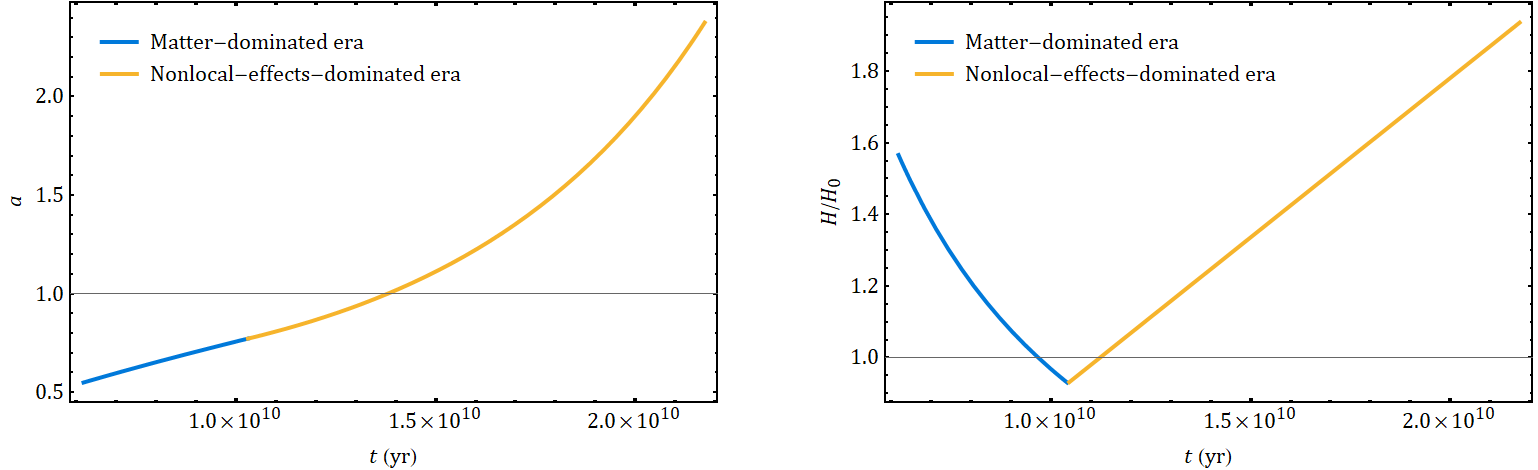
Figure 1: The evolution of the scale factor (on the left) and the Hubble parameter normalized with respect to the Hubble constant (on the right) in the late Universe.

The parameter $\lambda$ can thus be fixed by requiring that the scale factor for the matter-dominated era ($a(t)\propto t^{2/3}$) and that for the subsequent accelerated expansion match at $t_{*}$. First of all, by imposing the boundary condition $a(t_{0})=a_{0}$, where $t_{0}=13.8$ Gyr is the current age of the Universe, one finds the expression

$$a(t)=a_{0}e^{\frac{\lambda}{2}(t^{2}-t_{0}^{2})};$$ (34)

then, the matching condition gives

$$a(t_{*})=a_{0}e^{\frac{\lambda}{2}(t_{*}^{2}-t_{0}^{2})}=a_{*}\Rightarrow\lambda=\frac{2\ln\bigl(\frac{a_{0}}{a_{*}}\bigr{missing})}{t_{0}^{2}-t_{*}^{2}},$$ (35)

that is $\lambda=6.14\cdot 10^{-3}$ Gyr${}^{-2}=2.67\cdot 10^{-84}$ GeV². Therefore, while $M_{\textup{P}}^{2}\sim 10^{37}$ GeV² is the UV mass scale, $M^{2}$ and $\lambda$ are both IR mass parameters with $M^{2}\sim\lambda\sim 10^{-84}$ GeV².

It is convenient to introduce the dimensionless time parameter $\tau\equiv\lambda t^{2}$, thereby $\tau(t_{*})\equiv\tau_{*}=0.651$ and $\tau(t_{0})\equiv\tau_{0}=1.17$. One finds

$$R(\tau) =12\lambda\tau+6\lambda,$$ (36)

$$(\Box R)(\tau) =-72\lambda^{2}\tau-24\lambda^{2},$$ (37)

$$(\Box^{-1}R)(\tau) =-\tau\biggl{[}2+{}_{2}F_{2}\biggl{(}1,1;\frac{3}{2},2;-\frac{3}{2}\tau\biggr{)}\biggr{]},$$ (38)

where ${}_{2}F_{2}$ is a generalised hypergeometric function. This scale factor does not satisfy exactly the ansatz (17). However, in the interval $\tau_{*}\leq\tau\leq\tau_{0}$, the function ${}_{2}F_{2}$ is slowly-varying in time and thus approximates with its mean value $\approx 2/3$. See FIG. 2. It is worth noticing that the relative errors are less than 3%.

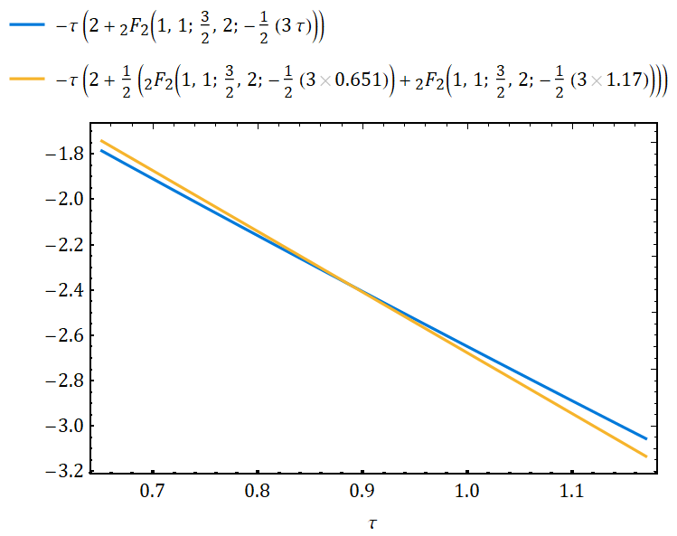
Figure 2: Comparison of $(\Box^{-1}R)(\tau)$ and its approximation in the time interval $\tau_{*}\leq\tau\leq\tau_{0}$.

As a result, the values of the parameters for which the ansatz (17) is approximately verified are

$$r_{1}\approx-\frac{2}{9\lambda}\equiv\frac{1}{\bar{\lambda}},\qquad r_{2}\approx\frac{4}{3}.$$ (39)

From Eqs. (18) and (19), we see that this result implies

$$\Box^{-n}R =\bar{\lambda}^{-n}(R-6\lambda),$$ (40)

$$\bar{\mathcal{F}}_{1}(\Box)R=(R-6\lambda)\sum_{n=1}^{\infty}f_{1_{-n}}\bar{\lambda}^{-n} =(R-6\lambda)\sum_{n=1}^{\infty}\tilde{f}_{1_{-n}}\biggl{(}\frac{M^{2}}{\bar{\lambda}}\biggr{)}^{n}=\bar{\mathcal{F}}_{1}(\bar{\lambda})(R-6\lambda)\,,$$ (41)

which we are going to discuss. An important remark is in order at this point. A similar line of attack of the problem can be adopted also at UV scale. See for example Spyridon ; biswas2 .

IV Dark energy as a nonlocal gravitational effect

Substituting the result (41) into the nonlocal action (1) yields

$$S=\int d^{4}x\,\frac{\sqrt{-g}}{2}\bigl{\{}[M_{\textup{P}}^{2}-6\lambda\bar{\mathcal{F}}_{1}(\bar{\lambda})]R+\bar{\mathcal{F}}_{1}(\bar{\lambda})R^{2}\bigr{\}}.$$ (42)

This expression shows that, for the particular solution (34), this Infinite Derivative Gravity model represents a correction to the Starobinsky model, whose action can be expressed as

$$S=\int d^{4}x\,\frac{\sqrt{-g}}{2}M_{\textup{P}}^{2}(R+\alpha R^{2}).$$ (43)

The nonlocal effects, contained in the dimensionless coefficient $\bar{\mathcal{F}}_{1}(\bar{\lambda})$, act both as a correction to the gravitational constant (and therefore to Einstein’s General Relativity) and as a dynamical source for the $R^{2}$ term of Starobinsky gravity.

The coefficient $\bar{\mathcal{F}}_{1}(\bar{\lambda})$ remains to be determined. One possibility is to compute all the coefficients $\tilde{f}_{1_{-n}}$ and then add them up as follows:

$$\begin{split}\bar{\mathcal{F}}_{1}(\bar{\lambda})=\sum_{n=1}^{\infty}\tilde{f}_{1_{-n}}\biggl{(}\frac{M^{2}}{\bar{\lambda}}\biggr{)}^{n}&\approx-\frac{2M^{2}}{9\lambda}\tilde{f}_{1_{-1}}+\frac{4M^{4}}{81\lambda^{2}}\tilde{f}_{1_{-2}}-\frac{8M^{6}}{729\lambda^{3}}\tilde{f}_{1_{-3}}+\frac{16M^{8}}{6561\lambda^{4}}\tilde{f}_{1_{-4}}-\dots\\ &\approx-0.0832\tilde{f}_{1_{-1}}+0.00693\tilde{f}_{1_{-2}}-0.000577\tilde{f}_{1_{-3}}+0.0000480\tilde{f}_{1_{-4}}-\dots.\,,\end{split}$$ (44)

where we have retained three significant figures. Substituting Eqs.(34) and (39) into cosmological Eqs. (27) and (28) gives respectively

$$M_{\textup{P}}^{2}\lambda(2+3\tau)+48\bar{\mathcal{F}}_{1}(\bar{\lambda})\lambda^{2}(1+4\tau)+8\lambda^{2}\tau(8+9\tau)\sum_{n=1}^{\infty}nf_{1_{-n}}\bar{\lambda}^{-n}=0$$ (45)

and

$$M_{\textup{P}}^{2}\lambda(1+2\tau)+24\bar{\mathcal{F}}_{1}(\bar{\lambda})\lambda^{2}(1+4\tau)+\frac{16}{3}\lambda^{2}\tau(4+9\tau)\sum_{n=1}^{\infty}nf_{1_{-n}}\bar{\lambda}^{-n}=\frac{1}{6}\Omega_{m}\rho_{c}e^{-\frac{3}{2}(\tau-\tau_{0})}.$$ (46)

The last two equations are constraints for the coefficients $\tilde{f}_{1_{-n}}$. First of all, it must be clarified why these equations contain the time variable $\tau$, whereas they should constrain some constant quantities; this is the case because the ansatz (17) is only approximately satisfied, in particular it is satisfied only if a slowly-varying function of time (the generalised hypergeometric function ${}_{2}F_{2}$) is neglected: as a consequence, also the coefficients $\tilde{f}_{1_{-n}}$ should be some slowly-varying functions of time, in such a way that they can still be regarded as almost constant during the cosmological era of interest. Secondly, Eqs. (45) and (46) are two constraints whereby an infinite set of parameters, i.e. the coefficients $\tilde{f}_{1_{-n}}$, cannot be completely determined.

A theory with an infinite number of free parameters – that cannot even be predicted – is devoid of physical meaning. From a practical point of view, it must exist the possibility to reformulate it in an alternative form containing a finite number of parameters to avoid infinite fine-tunings.

An approach is to calculate the dimensionless quantity $\bar{\mathcal{F}}_{1}(\bar{\lambda})$, since the nonlocal corrections can be rewritten in terms of this function only. It is a power series with unknown coefficients $\tilde{f}_{1_{-n}}$ and base $\frac{M^{2}}{\bar{\lambda}}$. If all of the infinite coefficients are of the same order of magnitude with alternating signs, it is a Leibniz series implying that $\bar{\mathcal{F}}_{1}(\bar{\lambda})$ is converging. We have to consider that $\absolutevalue{\frac{M^{2}}{\bar{\lambda}}}=\frac{2M^{2}}{9\lambda}\sim\frac{1}{12}$. Secondly, cosmological Eqs. (45) and (46) constitute nonlinear constraints for $\bar{\mathcal{F}}_{1}(\bar{\lambda})$ and thus they cannot provide a general closed form for such coefficient.

A different approach to calculate $\bar{\mathcal{F}}_{1}(\bar{\lambda})$ is not considering coefficients $\tilde{f}_{1_{-n}}$ and going back to the nonlocal action (42) obtained for the cosmological solution (34). Assuming the Starobinsky gravity (43), one can define

$$\bar{\mathcal{F}}_{1}(\bar{\lambda})\equiv M_{\textup{P}}^{2}\alpha,$$ (47)

so that the action (42) can be put into a more concise form:

$$S=\int d^{4}x\,\frac{\sqrt{-g}}{2}M_{\textup{P}}^{2}[(1-6\alpha\lambda)R+\alpha R^{2}].$$ (48)

The field equations obtained from the variational principle are a straightforward generalisation of those of Starobinsky gravity, that is:

$$(1-6\alpha\lambda)G_{\mu\nu}+2\alpha\biggl{(}RR_{\mu\nu}-\frac{1}{4}g_{\mu\nu}R^{2}+g_{\mu\nu}\Box R-\nabla_{\mu}\nabla_{\nu}R\biggr{)}=M_{\textup{P}}^{-2}T_{\mu\nu}.$$ (49)

Also in this case, we are assuming that the coefficients $\tilde{f}_{1_{-n}}$ are slowly-varying functions of time, which means that the quantity $\alpha$ can be considered as effectively constant during the cosmological era of interest.

The trace equation of Eqs. (49) is

$$6\alpha\Box R-(1-6\alpha\lambda)R=M_{\textup{P}}^{-2}T.$$ (50)

Substituting expressions (36) and (37), one finds

$$\alpha=\frac{M_{\textup{P}}^{-2}T+R}{6(\lambda+\Box)R}=\frac{\frac{\Omega_{m}\rho_{c}}{6M_{\textup{P}}^{2}\lambda}e^{-\frac{3}{2}(\tau-\tau_{0})}-2\tau-1}{6\lambda(10\tau+3)},$$ (51)

which, when evaluated at the present cosmic time, yields the following result:

$$\alpha=\frac{\frac{\Omega_{m}\rho_{c}}{6M_{\textup{P}}^{2}\lambda}-2\tau_{0}-1}{6\lambda(10\tau_{0}+3)},$$ (52)

that is $\alpha=-1.37\cdot 10^{82}$ GeV^-2. This implies that

$$\bar{\mathcal{F}}_{1}(\bar{\lambda})=\frac{\frac{\Omega_{m}\rho_{c}}{6\lambda}-M_{\textup{P}}^{2}(2\tau_{0}+1)}{6\lambda(10\tau_{0}+3)}$$ (53)

and so $\bar{\mathcal{F}}_{1}(\bar{\lambda})=-8.14\cdot 10^{118}$.

Let us discuss this result in view of the nonlocal action (42). The coefficient of the first term, the one proportional to $R$, is $M_{\textup{P}}^{2}-6\lambda\bar{\mathcal{F}}_{1}(\bar{\lambda})=7.26\cdot 10^{36}$ GeV²$=1.22\,M_{\textup{P}}^{2}$; in particular, the result $\bar{\mathcal{F}}_{1}(\bar{\lambda})<0$ implies a decrease of the effective gravitational constant in the current cosmological era, i.e. $G\rightarrow G_{\textup{eff}}=G/1.22=82\%\,G$, thereby possibly explaining dark energy away as the manifestation of nonlocal gravitational effects on cosmological scales. These nonlocal effects can thus be regarded either as repulsive gravity (in the sense of spacetime curvature) or as negative pressure (in the sense of matter sources).

The coefficient of the second term, the one proportional to $R^{2}$, is $\bar{\mathcal{F}}_{1}(\bar{\lambda})$, whose negative sign could hint at the presence of ghosts in the theory: that is the case in a Minkowski background biswas:propagator , but it has yet to be demonstrated in a curved spacetime as well. Furthermore, in the Starobinsky model, the parameter $\alpha$ corresponds to a mass being $m=1/\sqrt{-6\alpha}$, yielding $m\sim 10^{-42}$ GeV$\sim H_{0}$, so the sum of the nonlocal series can be physically interpreted as proportional to the mass of a (very light) scalar field.

V Discussion and Conclusions

The present analysis shows that it is possible to describe a dark energy behavior in the context of Infinite Derivative Gravity, considered as an effective theory of gravity with nonlocal effects. This represents an alternative picture to the addition of the cosmological constant term in General Relativity or to the introduction of some unknown scalar fields. In particular, the considered phenomenological model provides an accelerated expansion of the late Universe without affecting the evolution of the previous cosmological eras, as the nonlocal effects are significant only in the IR limit.

Interestingly, the model also predicts a reduction of the effective gravitational constant in the current cosmological era: therefore, it could be possible that, after the matter-dominated era, the evolution of the Universe is driven by the emergence of nonlocal gravitational effects, which remain ‘hidden’ until the Universe has cooled enough. See also vanPutten2 . This conclusion points out the fact that General Relativity is valid with great accuracy in the energy interval between the IR limit, set by $M$, where nonlocal effects become dominant, and the UV limit, set by $M_{\textup{P}}$, where quantum effects take over. At cosmological scales, results from the JWST and Euclid missions could be indicative in this direction. See, e.g. JWST ; vanPutten3 .

Moreover, one should not overlook that the present analysis indicates that Infinite Derivative Gravity can be predictive without resorting to a truncation of its infinitely many derivative terms, which play a crucial role for the quantization of the theory biswas:towards . Besides the applications in the IR limit, the formalism outlined here can be applied also in the UV limit, considering, in particular, the Starobinsky inflation and the primordial cosmological perturbations. These topics will be developed in a forthcoming study.

Aknowledgements

This paper is based upon work from the COST Action CA21136, “Addressing observational tensions in cosmology with systematics and fundamental physics” (CosmoVerse) supported by COST (European Cooperation in Science and Technology). SC and GM acknowledge the support by Istituto Nazionale di Fisica Nucleare, Sez. di Napoli, Iniziativa Specifica QGSKY.

*

Appendix A Derivation of the nonlocal cosmological equations

Here we provide an in-depth calculation of nonlocal cosmological Eqs. (A20) and (A21). The nonzero components of the Ricci tensor in the flat Friedmann–Lemaître–Robertson–Walker metric (11) are

$$R_{00}=-3\frac{\ddot{a}}{a},\qquad R_{11}=R_{22}=R_{33}=a\ddot{a}+2\dot{a}^{2}.$$ (A1)

Thus, making use of the expression (12) for the Ricci scalar, we have that the ‘00’-component and the ‘11’-component of the Einstein tensor are given respectively by

$$G_{00}=R_{00}-\frac{1}{2}g_{00}R=3\frac{\dot{a}^{2}}{a^{2}},\qquad G_{11}=R_{11}-\frac{1}{2}g_{11}R=-2a\ddot{a}-\dot{a}^{2}.$$ (A2)

The stress-energy tensor for a perfect fluid in the metric (11) is given by

$$T_{\mu}^{\nu}=\operatorname{diag}\Bigl{(}-\rho(t),p(t),p(t),p(t)\Bigr{)},$$ (A3)

so its relevant components are

$$T_{00}=\rho,\qquad T_{11}=a^{2}p.$$ (A4)

Furthermore, considering that

$$\bar{\mathcal{F}}_{1}(\Box)R =6\sum_{n=1}^{\infty}f_{1_{-n}}\Box^{-n}\biggl{(}\frac{a\ddot{a}+\dot{a}^{2}}{a^{2}}\biggr{)},$$ (A5)

$$\Theta_{\mu\nu}^{1} =36\delta_{\mu}^{0}\delta_{\nu}^{0}\sum_{n=1}^{\infty}f_{1_{-n}}\sum_{l=0}^{n-1}\partial_{0}\Box^{-l-1}\biggl{(}\frac{a\ddot{a}+\dot{a}^{2}}{a^{2}}\biggr{)}\partial_{0}\Box^{-n+l}\biggl{(}\frac{a\ddot{a}+\dot{a}^{2}}{a^{2}}\biggr{)},$$ (A6)

$$\Theta_{\sigma}^{1\sigma} =g^{\mu\nu}\Theta_{\mu\nu}^{1}=-36\sum_{n=1}^{\infty}f_{1_{-n}}\sum_{l=0}^{n-1}\partial_{0}\Box^{-l-1}\biggl{(}\frac{a\ddot{a}+\dot{a}^{2}}{a^{2}}\biggr{)}\partial_{0}\Box^{-n+l}\biggl{(}\frac{a\ddot{a}+\dot{a}^{2}}{a^{2}}\biggr{)},$$ (A7)

$$\bar{\Theta}^{1} =36\sum_{n=1}^{\infty}f_{1_{-n}}\sum_{l=0}^{n-1}\Box^{-l-1}\biggl{(}\frac{a\ddot{a}+\dot{a}^{2}}{a^{2}}\biggr{)}\Box^{-n+l+1}\biggl{(}\frac{a\ddot{a}+\dot{a}^{2}}{a^{2}}\biggr{)},$$ (A8)

$$\partial_{0}R =6\frac{a^{2}\dddot{a}+a\dot{a}\ddot{a}-2\dot{a}^{3}}{a^{3}},$$ (A9)

$$\Box R =-6a^{-3}\partial_{0}\biggl{(}a^{3}\partial_{0}\frac{a\ddot{a}+\dot{a}^{2}}{a^{2}}\biggr{)}=-6\frac{a\ddot{a}^{2}-5\dot{a}^{2}\ddot{a}+3a\dot{a}\dddot{a}+a^{2}\ddddot{a}}{a^{3}},$$ (A10)

the ‘00’-component and the ‘11’-component of field Eqs. (6) can be rewritten respectively as

$$T_{00} =M_{\textup{P}}^{2}G_{00}+2G_{00}\bar{\mathcal{F}}_{1}(\Box)R+\frac{1}{2}g_{00}R\bar{\mathcal{F}}_{1}(\Box)R+\Theta_{00}^{1}-\frac{1}{2}g_{00}\bigl{(}\Theta_{\sigma}^{1\sigma}+\bar{\Theta}^{1}\bigr{)},$$ (A11a)

$$T_{11} =M_{\textup{P}}^{2}G_{11}+2G_{11}\bar{\mathcal{F}}_{1}(\Box)R+\frac{1}{2}g_{11}R\bar{\mathcal{F}}_{1}(\Box)R+2g_{11}\Box\bar{\mathcal{F}}_{1}(\Box)R-\frac{1}{2}g_{11}\bigl{(}\Theta_{\sigma}^{1\sigma}+\bar{\Theta}^{1}\bigr{)}$$ (A11b)

or, more explicitly, as

$$\begin{split}\rho&=3M_{\textup{P}}^{2}\frac{\dot{a}^{2}}{a^{2}}+18\biggl{(}-\frac{\ddot{a}}{a}+\frac{\dot{a}^{2}}{a^{2}}\biggr{)}\sum_{n=1}^{\infty}f_{1_{-n}}\Box^{-n}\biggl{(}\frac{a\ddot{a}+\dot{a}^{2}}{a^{2}}\biggr{)}\\ &+18\sum_{n=1}^{\infty}f_{1_{-n}}\sum_{l=0}^{n-1}\partial_{0}\Box^{-l-1}\biggl{(}\frac{a\ddot{a}+\dot{a}^{2}}{a^{2}}\biggr{)}\partial_{0}\Box^{-n+l}\biggl{(}\frac{a\ddot{a}+\dot{a}^{2}}{a^{2}}\biggr{)}+18\sum_{n=1}^{\infty}f_{1_{-n}}\sum_{l=0}^{n-1}\Box^{-l-1}\biggl{(}\frac{a\ddot{a}+\dot{a}^{2}}{a^{2}}\biggr{)}\Box^{-n+l+1}\biggl{(}\frac{a\ddot{a}+\dot{a}^{2}}{a^{2}}\biggr{)}\end{split}$$ (A12)

and

$$\begin{split}p&=-M_{\textup{P}}^{2}\biggl{(}2\frac{\ddot{a}}{a}+\frac{\dot{a}^{2}}{a^{2}}\biggr{)}+6\biggl{[}-\frac{\ddot{a}}{a}+\frac{\dot{a}^{2}}{a^{2}}-2a^{-3}\partial_{0}(a^{3}\partial_{0})\biggr{]}\sum_{n=1}^{\infty}f_{1_{-n}}\Box^{-n}\biggl{(}\frac{a\ddot{a}+\dot{a}^{2}}{a^{2}}\biggr{)}\\ &+18\sum_{n=1}^{\infty}f_{1_{-n}}\sum_{l=0}^{n-1}\partial_{0}\Box^{-l-1}\biggl{(}\frac{a\ddot{a}+\dot{a}^{2}}{a^{2}}\biggr{)}\partial_{0}\Box^{-n+l}\biggl{(}\frac{a\ddot{a}+\dot{a}^{2}}{a^{2}}\biggr{)}-18\sum_{n=1}^{\infty}f_{1_{-n}}\sum_{l=0}^{n-1}\Box^{-l-1}\biggl{(}\frac{a\ddot{a}+\dot{a}^{2}}{a^{2}}\biggr{)}\Box^{-n+l+1}\biggl{(}\frac{a\ddot{a}+\dot{a}^{2}}{a^{2}}\biggr{)}.\end{split}$$ (A13)

Using the equation of state, $p=w\rho$, Eqs. (A12) and (A13) can be combined into a single integro-differential equation for the scale factor:

$$\begin{split}&M_{\textup{P}}^{2}\biggl{[}2\frac{\ddot{a}}{a}+(3w+1)\frac{\dot{a}^{2}}{a^{2}}\biggr{]}-6\biggl{[}(3w-1)\biggl{(}\frac{\ddot{a}}{a}-\frac{\dot{a}^{2}}{a^{2}}\biggr{)}-2a^{-3}\partial_{0}(a^{3}\partial_{0})\biggr{]}\sum_{n=1}^{\infty}f_{1_{-n}}\Box^{-n}\biggl{(}\frac{a\ddot{a}+\dot{a}^{2}}{a^{2}}\biggr{)}\\ &+18(w-1)\sum_{n=1}^{\infty}f_{1_{-n}}\sum_{l=0}^{n-1}\partial_{0}\Box^{-l-1}\biggl{(}\frac{a\ddot{a}+\dot{a}^{2}}{a^{2}}\biggr{)}\partial_{0}\Box^{-n+l}\biggl{(}\frac{a\ddot{a}+\dot{a}^{2}}{a^{2}}\biggr{)}\\ &+18(w+1)\sum_{n=1}^{\infty}f_{1_{-n}}\sum_{l=0}^{n-1}\Box^{-l-1}\biggl{(}\frac{a\ddot{a}+\dot{a}^{2}}{a^{2}}\biggr{)}\Box^{-n+l+1}\biggl{(}\frac{a\ddot{a}+\dot{a}^{2}}{a^{2}}\biggr{)}=0.\end{split}$$ (A14)

Carrying out the same substitutions for trace Eq. (8), one obtains

$$\begin{split}M_{\textup{P}}^{2}\frac{a\ddot{a}+\dot{a}^{2}}{a^{2}}&+6a^{-3}\partial_{0}(a^{3}\partial_{0})\sum_{n=1}^{\infty}f_{1_{-n}}\Box^{-n}\biggl{(}\frac{a\ddot{a}+\dot{a}^{2}}{a^{2}}\biggr{)}-6\sum_{n=1}^{\infty}f_{1_{-n}}\sum_{l=0}^{n-1}\partial_{0}\Box^{-l-1}\biggl{(}\frac{a\ddot{a}+\dot{a}^{2}}{a^{2}}\biggr{)}\partial_{0}\Box^{-n+l}\biggl{(}\frac{a\ddot{a}+\dot{a}^{2}}{a^{2}}\biggr{)}\\ &+12\sum_{n=1}^{\infty}f_{1_{-n}}\sum_{l=0}^{n-1}\Box^{-l-1}\biggl{(}\frac{a\ddot{a}+\dot{a}^{2}}{a^{2}}\biggr{)}\Box^{-n+l+1}\biggl{(}\frac{a\ddot{a}+\dot{a}^{2}}{a^{2}}\biggr{)}=\frac{1-3w}{6}\rho.\end{split}$$ (A15)

The nonlocal operators appearing in Eqs. (A14) and (A15) can be evaluated as follows:

$$\biggl{[}\Box^{-1}\biggl{(}\frac{a\ddot{a}+\dot{a}^{2}}{a^{2}}\biggr{)}\biggr{]}(t) =-\int_{0}^{t}dt^{\prime}\,a^{-3}(t^{\prime})\int_{0}^{t^{\prime}}dt^{\prime\prime}\,(a^{2}\ddot{a}+a\dot{a}^{2})(t^{\prime\prime}),$$ (A16)

$$\biggl{[}\partial_{0}\Box^{-1}\biggl{(}\frac{a\ddot{a}+\dot{a}^{2}}{a^{2}}\biggr{)}\biggr{]}(t) =\biggl{[}\Box^{-1}\biggl{(}\frac{a^{2}\dddot{a}+a\dot{a}\ddot{a}-2\dot{a}^{3}}{a^{3}}\biggr{)}\biggr{]}(t)=-\int_{0}^{t}dt^{\prime}\,a^{-3}(t^{\prime})\int_{0}^{t^{\prime}}dt^{\prime\prime}\,(a^{2}\dddot{a}+a\dot{a}\ddot{a}-2\dot{a}^{3})(t^{\prime\prime}).$$ (A17)

By recursive application of the operator $\Box^{-1}$, from Eqs. (A16) and (A17), one finds respectively that

$$\biggl{[}\Box^{-n}\biggl{(}\frac{a\ddot{a}+\dot{a}^{2}}{a^{2}}\biggr{)}\biggr{]}(t)$$

$$=(-1)^{n}\int_{0}^{t}dt^{\prime}\,a^{-3}(t^{\prime})\int_{0}^{t^{\prime}}dt^{\prime\prime}\,a^{3}(t^{\prime\prime})\dots\int_{0}^{t^{(2n-2)}}dt^{(2n-1)}\,a^{-3}\bigl{(}t^{(2n-1)}\bigr{)}\int_{0}^{t^{(2n-1)}}dt^{(2n)}\,(a^{2}\ddot{a}+a\dot{a}^{2})\bigl{(}t^{(2n)}\bigr{)},$$ (A18)

$$\biggl{[}\partial_{0}\Box^{-n}\biggl{(}\frac{a\ddot{a}+\dot{a}^{2}}{a^{2}}\biggr{)}\biggr{]}(t)=\biggl{[}\Box^{-n}\biggl{(}\frac{a^{2}\dddot{a}+a\dot{a}\ddot{a}-2\dot{a}^{3}}{a^{3}}\biggr{)}\biggr{]}(t)$$

$$=(-1)^{n}\int_{0}^{t}dt^{\prime}\,a^{-3}(t^{\prime})\int_{0}^{t^{\prime}}dt^{\prime\prime}\,a^{3}(t^{\prime\prime})\dots\int_{0}^{t^{(2n-2)}}dt^{(2n-1)}\,a^{-3}\bigl{(}t^{(2n-1)}\bigr{)}\int_{0}^{t^{(2n-1)}}dt^{(2n)}\,(a^{2}\dddot{a}+a\dot{a}\ddot{a}-2\dot{a}^{3})\bigl{(}t^{(2n)}\bigr{)},$$ (A19)

where both expressions contain $2n$ time integrals with $2n$ variables of integration $t^{\prime},t^{\prime\prime},\dots,t^{(2n-1)},t^{(2n)}$. Finally, substituting the results (A) and (A) into Eqs. (A14) and (A15) yields

$$\begin{split}&0=M_{\textup{P}}^{2}\biggl{[}2\frac{\ddot{a}}{a}+(3w+1)\frac{\dot{a}^{2}}{a^{2}}\biggr{]}-6\biggl{[}(3w-1)\biggl{(}\frac{\ddot{a}}{a}-\frac{\dot{a}^{2}}{a^{2}}\biggr{)}-2a^{-3}\partial_{0}(a^{3}\partial_{0})\biggr{]}\Biggl{\{}\sum_{n=1}^{\infty}(-1)^{n}f_{1_{-n}}\\ &\cdot\Biggl{[}\int_{0}^{t}dt^{\prime}\,a^{-3}(t^{\prime})\int_{0}^{t^{\prime}}dt^{\prime\prime}\,a^{3}(t^{\prime\prime})\dots\int_{0}^{t^{(2n-2)}}dt^{(2n-1)}\,a^{-3}\bigl{(}t^{(2n-1)}\bigr{)}\int_{0}^{t^{(2n-1)}}dt^{(2n)}\,(a^{2}\ddot{a}+a\dot{a}^{2})\bigl{(}t^{(2n)}\bigr{)}\Biggr{]}\Biggr{\}}\\ &+18(w-1)\Biggl{\{}\sum_{n=1}^{\infty}(-1)^{n+1}f_{1_{-n}}\\ &\cdot\sum_{l=0}^{n-1}\Biggl{[}\int_{0}^{t}dt^{\prime}\,a^{-3}(t^{\prime})\int_{0}^{t^{\prime}}dt^{\prime\prime}\,a^{3}(t^{\prime\prime})\dots\int_{0}^{t^{(2l)}}dt^{(2l+1)}\,a^{-3}\bigl{(}t^{(2l+1)}\bigr{)}\int_{0}^{t^{(2l+1)}}dt^{(2l+2)}\,(a^{2}\dddot{a}+a\dot{a}\ddot{a}-2\dot{a}^{3})\bigl{(}t^{(2l+2)}\bigr{)}\Biggr{]}\\ &\cdot\Biggl{[}\int_{0}^{t}dt^{\prime}\,a^{-3}(t^{\prime})\int_{0}^{t^{\prime}}dt^{\prime\prime}\,a^{3}(t^{\prime\prime})\dots\int_{0}^{t^{(2n-2l-2)}}dt^{(2n-2l-1)}\,a^{-3}\bigl{(}t^{(2n-2l-1)}\bigr{)}\int_{0}^{t^{(2n-2l-1)}}dt^{(2n-2l)}\,(a^{2}\dddot{a}+a\dot{a}\ddot{a}-2\dot{a}^{3})\bigl{(}t^{(2n-2l)}\bigr{)}\Biggr{]}\Biggr{\}}\\ &+18(w+1)\Biggl{\{}\sum_{n=1}^{\infty}(-1)^{n+1}f_{1_{-n}}\\ &\cdot\sum_{l=0}^{n-1}\Biggl{[}\int_{0}^{t}dt^{\prime}\,a^{-3}(t^{\prime})\int_{0}^{t^{\prime}}dt^{\prime\prime}\,a^{3}(t^{\prime\prime})\dots\int_{0}^{t^{(2l)}}dt^{(2l+1)}\,a^{-3}\bigl{(}t^{(2l+1)}\bigr{)}\int_{0}^{t^{(2l+1)}}dt^{(2l+2)}\,(a^{2}\ddot{a}+a\dot{a}^{2})\bigl{(}t^{(2l+2)}\bigr{)}\Biggr{]}\\ &\cdot\Biggl{[}\int_{0}^{t}dt^{\prime}\,a^{-3}(t^{\prime})\int_{0}^{t^{\prime}}dt^{\prime\prime}\,a^{3}(t^{\prime\prime})\dots\int_{0}^{t^{(2n-2l-4)}}dt^{(2n-2l-3)}\,a^{-3}\bigl{(}t^{(2n-2l-3)}\bigr{)}\int_{0}^{t^{(2n-2l-3)}}dt^{(2n-2l-2)}\,(a^{2}\ddot{a}+a\dot{a}^{2})\bigl{(}t^{(2n-2l-2)}\bigr{)}\Biggr{]}\Biggr{\}}\end{split}$$ (A20)

and

$$\begin{split}&\frac{1-3w}{6}\rho=M_{\textup{P}}^{2}\frac{a\ddot{a}+\dot{a}^{2}}{a^{2}}+6a^{-3}\partial_{0}(a^{3}\partial_{0})\Biggl{\{}\sum_{n=1}^{\infty}(-1)^{n}f_{1_{-n}}\\ &\cdot\Biggl{[}\int_{0}^{t}dt^{\prime}\,a^{-3}(t^{\prime})\int_{0}^{t^{\prime}}dt^{\prime\prime}\,a^{3}(t^{\prime\prime})\dots\int_{0}^{t^{(2n-2)}}dt^{(2n-1)}\,a^{-3}\bigl{(}t^{(2n-1)}\bigr{)}\int_{0}^{t^{(2n-1)}}dt^{(2n)}\,(a^{2}\ddot{a}+a\dot{a}^{2})\bigl{(}t^{(2n)}\bigr{)}\Biggr{]}\Biggr{\}}\\ &-6\Biggl{\{}\sum_{n=1}^{\infty}(-1)^{n+1}f_{1_{-n}}\\ &\cdot\sum_{l=0}^{n-1}\Biggl{[}\int_{0}^{t}dt^{\prime}\,a^{-3}(t^{\prime})\int_{0}^{t^{\prime}}dt^{\prime\prime}\,a^{3}(t^{\prime\prime})\dots\int_{0}^{t^{(2l)}}dt^{(2l+1)}\,a^{-3}\bigl{(}t^{(2l+1)}\bigr{)}\int_{0}^{t^{(2l+1)}}dt^{(2l+2)}\,(a^{2}\dddot{a}+a\dot{a}\ddot{a}-2\dot{a}^{3})\bigl{(}t^{(2l+2)}\bigr{)}\Biggr{]}\\ &\cdot\Biggl{[}\int_{0}^{t}dt^{\prime}\,a^{-3}(t^{\prime})\int_{0}^{t^{\prime}}dt^{\prime\prime}\,a^{3}(t^{\prime\prime})\dots\int_{0}^{t^{(2n-2l-2)}}dt^{(2n-2l-1)}\,a^{-3}\bigl{(}t^{(2n-2l-1)}\bigr{)}\int_{0}^{t^{(2n-2l-1)}}dt^{(2n-2l)}\,(a^{2}\dddot{a}+a\dot{a}\ddot{a}-2\dot{a}^{3})\bigl{(}t^{(2n-2l)}\bigr{)}\Biggr{]}\Biggr{\}}\\ &+12\Biggl{\{}\sum_{n=1}^{\infty}(-1)^{n+1}f_{1_{-n}}\\ &\cdot\sum_{l=0}^{n-1}\Biggl{[}\int_{0}^{t}dt^{\prime}\,a^{-3}(t^{\prime})\int_{0}^{t^{\prime}}dt^{\prime\prime}\,a^{3}(t^{\prime\prime})\dots\int_{0}^{t^{(2l)}}dt^{(2l+1)}\,a^{-3}\bigl{(}t^{(2l+1)}\bigr{)}\int_{0}^{t^{(2l+1)}}dt^{(2l+2)}\,(a^{2}\ddot{a}+a\dot{a}^{2})\bigl{(}t^{(2l+2)}\bigr{)}\Biggr{]}\\ &\cdot\Biggl{[}\int_{0}^{t}dt^{\prime}\,a^{-3}(t^{\prime})\int_{0}^{t^{\prime}}dt^{\prime\prime}\,a^{3}(t^{\prime\prime})\dots\int_{0}^{t^{(2n-2l-4)}}dt^{(2n-2l-3)}\,a^{-3}\bigl{(}t^{(2n-2l-3)}\bigr{)}\int_{0}^{t^{(2n-2l-3)}}dt^{(2n-2l-2)}\,(a^{2}\ddot{a}+a\dot{a}^{2})\bigl{(}t^{(2n-2l-2)}\bigr{)}\Biggr{]}\Biggr{\}}.\end{split}$$ (A21)

In the matter-dominated era, nonlocal cosmological Eqs. (A20) and (A21) become respectively

$$\begin{split}&0=M_{\textup{P}}^{2}\biggl{[}2\frac{\ddot{a}}{a}+(3w+1)\frac{\dot{a}^{2}}{a^{2}}\biggr{]}-6\biggl{[}-\frac{\ddot{a}}{a}+\frac{\dot{a}^{2}}{a^{2}}-2a^{-3}\partial_{0}(a^{3}\partial_{0})\biggr{]}\Biggl{\{}\sum_{n=1}^{\infty}(-1)^{n}f_{1_{-n}}\\ &\cdot\Biggl{[}\int_{0}^{t}dt^{\prime}\,a^{-3}(t^{\prime})\int_{0}^{t^{\prime}}dt^{\prime\prime}\,a^{3}(t^{\prime\prime})\dots\int_{0}^{t^{(2n-2)}}dt^{(2n-1)}\,a^{-3}\bigl{(}t^{(2n-1)}\bigr{)}\int_{0}^{t^{(2n-1)}}dt^{(2n)}\,(a^{2}\ddot{a}+a\dot{a}^{2})\bigl{(}t^{(2n)}\bigr{)}\Biggr{]}\Biggr{\}}\\ &-18\Biggl{\{}\sum_{n=1}^{\infty}(-1)^{n+1}f_{1_{-n}}\\ &\cdot\sum_{l=0}^{n-1}\Biggl{[}\int_{0}^{t}dt^{\prime}\,a^{-3}(t^{\prime})\int_{0}^{t^{\prime}}dt^{\prime\prime}\,a^{3}(t^{\prime\prime})\dots\int_{0}^{t^{(2l)}}dt^{(2l+1)}\,a^{-3}\bigl{(}t^{(2l+1)}\bigr{)}\int_{0}^{t^{(2l+1)}}dt^{(2l+2)}\,(a^{2}\dddot{a}+a\dot{a}\ddot{a}-2\dot{a}^{3})\bigl{(}t^{(2l+2)}\bigr{)}\Biggr{]}\\ &\cdot\Biggl{[}\int_{0}^{t}dt^{\prime}\,a^{-3}(t^{\prime})\int_{0}^{t^{\prime}}dt^{\prime\prime}\,a^{3}(t^{\prime\prime})\dots\int_{0}^{t^{(2n-2l-2)}}dt^{(2n-2l-1)}\,a^{-3}\bigl{(}t^{(2n-2l-1)}\bigr{)}\int_{0}^{t^{(2n-2l-1)}}dt^{(2n-2l)}\,(a^{2}\dddot{a}+a\dot{a}\ddot{a}-2\dot{a}^{3})\bigl{(}t^{(2n-2l)}\bigr{)}\Biggr{]}\Biggr{\}}\\ &+18\Biggl{\{}\sum_{n=1}^{\infty}(-1)^{n+1}f_{1_{-n}}\\ &\cdot\sum_{l=0}^{n-1}\Biggl{[}\int_{0}^{t}dt^{\prime}\,a^{-3}(t^{\prime})\int_{0}^{t^{\prime}}dt^{\prime\prime}\,a^{3}(t^{\prime\prime})\dots\int_{0}^{t^{(2l)}}dt^{(2l+1)}\,a^{-3}\bigl{(}t^{(2l+1)}\bigr{)}\int_{0}^{t^{(2l+1)}}dt^{(2l+2)}\,(a^{2}\ddot{a}+a\dot{a}^{2})\bigl{(}t^{(2l+2)}\bigr{)}\Biggr{]}\\ &\cdot\Biggl{[}\int_{0}^{t}dt^{\prime}\,a^{-3}(t^{\prime})\int_{0}^{t^{\prime}}dt^{\prime\prime}\,a^{3}(t^{\prime\prime})\dots\int_{0}^{t^{(2n-2l-4)}}dt^{(2n-2l-3)}\,a^{-3}\bigl{(}t^{(2n-2l-3)}\bigr{)}\int_{0}^{t^{(2n-2l-3)}}dt^{(2n-2l-2)}\,(a^{2}\ddot{a}+a\dot{a}^{2})\bigl{(}t^{(2n-2l-2)}\bigr{)}\Biggr{]}\Biggr{\}}\end{split}$$ (A22)

and

$$\begin{split}&\frac{1}{6}\Omega_{m}\rho_{c}a_{0}^{3}a^{-3}=M_{\textup{P}}^{2}\frac{a\ddot{a}+\dot{a}^{2}}{a^{2}}+6a^{-3}\partial_{0}(a^{3}\partial_{0})\Biggl{\{}\sum_{n=1}^{\infty}(-1)^{n}f_{1_{-n}}\\ &\cdot\Biggl{[}\int_{0}^{t}dt^{\prime}\,a^{-3}(t^{\prime})\int_{0}^{t^{\prime}}dt^{\prime\prime}\,a^{3}(t^{\prime\prime})\dots\int_{0}^{t^{(2n-2)}}dt^{(2n-1)}\,a^{-3}\bigl{(}t^{(2n-1)}\bigr{)}\int_{0}^{t^{(2n-1)}}dt^{(2n)}\,(a^{2}\ddot{a}+a\dot{a}^{2})\bigl{(}t^{(2n)}\bigr{)}\Biggr{]}\Biggr{\}}\\ &-6\Biggl{\{}\sum_{n=1}^{\infty}(-1)^{n+1}f_{1_{-n}}\\ &\cdot\sum_{l=0}^{n-1}\Biggl{[}\int_{0}^{t}dt^{\prime}\,a^{-3}(t^{\prime})\int_{0}^{t^{\prime}}dt^{\prime\prime}\,a^{3}(t^{\prime\prime})\dots\int_{0}^{t^{(2l)}}dt^{(2l+1)}\,a^{-3}\bigl{(}t^{(2l+1)}\bigr{)}\int_{0}^{t^{(2l+1)}}dt^{(2l+2)}\,(a^{2}\dddot{a}+a\dot{a}\ddot{a}-2\dot{a}^{3})\bigl{(}t^{(2l+2)}\bigr{)}\Biggr{]}\\ &\cdot\Biggl{[}\int_{0}^{t}dt^{\prime}\,a^{-3}(t^{\prime})\int_{0}^{t^{\prime}}dt^{\prime\prime}\,a^{3}(t^{\prime\prime})\dots\int_{0}^{t^{(2n-2l-2)}}dt^{(2n-2l-1)}\,a^{-3}\bigl{(}t^{(2n-2l-1)}\bigr{)}\int_{0}^{t^{(2n-2l-1)}}dt^{(2n-2l)}\,(a^{2}\dddot{a}+a\dot{a}\ddot{a}-2\dot{a}^{3})\bigl{(}t^{(2n-2l)}\bigr{)}\Biggr{]}\Biggr{\}}\\ &+12\Biggl{\{}\sum_{n=1}^{\infty}(-1)^{n+1}f_{1_{-n}}\\ &\cdot\sum_{l=0}^{n-1}\Biggl{[}\int_{0}^{t}dt^{\prime}\,a^{-3}(t^{\prime})\int_{0}^{t^{\prime}}dt^{\prime\prime}\,a^{3}(t^{\prime\prime})\dots\int_{0}^{t^{(2l)}}dt^{(2l+1)}\,a^{-3}\bigl{(}t^{(2l+1)}\bigr{)}\int_{0}^{t^{(2l+1)}}dt^{(2l+2)}\,(a^{2}\ddot{a}+a\dot{a}^{2})\bigl{(}t^{(2l+2)}\bigr{)}\Biggr{]}\\ &\cdot\Biggl{[}\int_{0}^{t}dt^{\prime}\,a^{-3}(t^{\prime})\int_{0}^{t^{\prime}}dt^{\prime\prime}\,a^{3}(t^{\prime\prime})\dots\int_{0}^{t^{(2n-2l-4)}}dt^{(2n-2l-3)}\,a^{-3}\bigl{(}t^{(2n-2l-3)}\bigr{)}\int_{0}^{t^{(2n-2l-3)}}dt^{(2n-2l-2)}\,(a^{2}\ddot{a}+a\dot{a}^{2})\bigl{(}t^{(2n-2l-2)}\bigr{)}\Biggr{]}\Biggr{\}}.\end{split}$$ (A23)

References

- (1) E. Abdalla, G. Franco Abellán, A. Aboubrahim, A. Agnello, O. Akarsu, Y. Akrami, G. Alestas, D. Aloni, L. Amendola and L. A. Anchordoqui, et al., Cosmology intertwined: A review of the particle physics, astrophysics, and cosmology associated with the cosmological tensions and anomalies, JHEAp 34, 49-211 (2022).
- (2) M. H. Goroff, A. Sagnotti, The ultraviolet behavior of Einstein gravity, Nucl. Phys. B 266, 709–736 (1986).
- (3) A. A. Starobinsky, A New Type of Isotropic Cosmological Models Without Singularity, Phys. Lett. B 91, 99-102 (1980).
- (4) A. D. Linde, Inflationary Cosmology, Inflationary Cosmology, 1–54 (2007).
- (5) A. H. Guth, Inflationary universe: A possible solution to the horizon and flatness problems, Phys. Rev. D 23, 347 (1981).
- (6) A. D. Linde, A new inflationary universe scenario: a possible solution of the horizon, flatness, homogeneity, isotropy and primordial monopole problems, Phys. Lett. B 108, 389–393 (1982).
- (7) A. D. Linde, Chaotic inflation, Phys. Lett. B 129, 177–181 (1983).
- (8) J. B. Hartle, S. W. Hawking, Wave function of the Universe, Phys. Rev. D 28 (1983).
- (9) A. Vilenkin, Quantum creation of universes, Phys. Rev. D 30, 509 (1984).
- (10) J. J. Halliwell, Introductory lectures on Quantum Cosmology, Quantum Cosmology and Baby Universes, 159–243 (1991).
-
(11)
M. H. P. M. van Putten,
-tension in the classical limit of Big Bang quantum cosmology,
32nd Texas Symp. Rel. Astroph., Shanghai, Session 7 (2023) [arXiv:2403.10865 [astro-ph.CO]] (2024). - (12) N. Aghanim et al., Planck Collaboration, Planck 2018 results. VI. Cosmological parameters, Astron. Astrophys. 641, A6 (2020).
- (13) S. Weinberg, The Cosmological Constant Problem, Rev. Mod. Phys. 61, 1–23 (1989).
- (14) A. Conroy, T. Koivisto, A. Mazumdar, A. Teimouri, Generalised Quadratic Curvature, Non-Local Infrared Modifications of Gravity and Newtonian Potentials, Class. Quant. Grav. 32, 015024 (2014).
- (15) M. H. P. M. van Putten, Entropic constraint on cosmic variation of Planck mass and the Boltzmann constant, Res. in Phys. 57, 107425 (2024).
- (16) S. Capozziello and M. Francaviglia, Extended Theories of Gravity and their Cosmological and Astrophysical Applications, Gen. Rel. Grav. 40, 357-420 (2008).
- (17) S. Nojiri, S. D. Odintsov and V. K. Oikonomou, Modified Gravity Theories on a Nutshell: Inflation, Bounce and Late-time Evolution, Phys. Rept. 692, 1-104 (2017).
- (18) S. Capozziello, F. Bajardi, Non-Local Gravity Cosmology: an Overview, Int. J. Mod. Phys. D (2022).
- (19) L. Modesto, Super-renormalizable gravity, The Thirteenth Marcel Grossmann Meeting: On Recent Developments in Theoretical and Experimental General Relativity, Astrophysics and Relativistic Field Theories, 1128–1130 (2015).
- (20) L. Modesto, Super-renormalizable quantum gravity, Phys. Rev. D 86, 044005 (2012).
- (21) F. Briscese, A. Marciano, L. Modesto, E. N. Saridakis, Inflation in (super-) renormalizable gravity, Phys. Rev. D 87, 083507 (2013).
- (22) T. Biswas, A. Mazumdar, W. Siegel, Bouncing Universes in String-inspired Gravity, J. Cosmol. Astropart. Phys. 03, 009 (2006).
- (23) L. Modesto, J. W. Moffat, P. Nicolini, Black holes in an ultraviolet complete quantum gravity, Phys. Lett. B 695, 397–400 (2011).
- (24) Yu. V. Kuzmin, The convergent nonlocal gravitation, Yad. Fiz. 50, 1630-1635 (1989).
- (25) E. T. Tomboulis, Superrenormalizable gauge and gravitational theories, [arXiv:hep-th/9702146 [hep-th]] (1997).
- (26) S. Talaganis, T. Biswas and A. Mazumdar, Towards understanding the ultraviolet behavior of quantum loops in infinite-derivative theories of gravity, Class. Quant. Grav. 32, 215017 (2015).
- (27) L. Buoninfante, A. Ghoshal, G. Lambiase and A. Mazumdar, Transmutation of nonlocal scale in infinite derivative field theories, Phys. Rev. D 99, 044032 (2019).
- (28) L. Buoninfante, G. Lambiase and M. Yamaguchi, Nonlocal generalization of Galilean theories and gravity, Phys. Rev. D 100, 026019 (2019).
- (29) T. Biswas, E. Gerwick, T. Koivisto, A. Mazumdar, Towards singularity-and ghost-free theories of gravity, Phys. Rev. Lett. 108, 031101 (2012).
- (30) L. Modesto and S. Tsujikawa, Non-local massive gravity, Phys. Lett. B 727 (2013), 48-56
- (31) M. Jaccard, M. Maggiore and E. Mitsou, Nonlocal theory of massive gravity, Phys. Rev. D 88, 044033 (2013).
- (32) S. Deser, R. P. Woodard, Nonlocal Cosmology, Phys. Rev. Lett. 99, 111301 (2007).
- (33) S. Deser, R. P. Woodard, Nonlocal Cosmology II – Cosmic acceleration without fine tuning or dark energy, J. Cosmol. Astropart. Phys. 06, 034 (2019).
- (34) N. Arkani-Hamed, S. Dimopoulos, G. Dvali, G. Gabadadze, Non-Local Modification of Gravity and the Cosmological Constant Problem, arXiv preprint hep-th/0209227 (2002).
- (35) A. O. Barvinsky, Nonlocal action for long-distance modifications of gravity theory, Phys. Lett. B 572, 109–116 (2003).
- (36) S. Nojiri, S. D. Odintsov, M. Sasaki, Y. Zhang, Screening of cosmological constant in non-local gravity, Phys. Lett. B 696, 278–282 (2011).
- (37) S. Nojiri, S. D. Odintsov and V. K. Oikonomou, Ghost-free non-local Gravity Cosmology, Phys. Dark Univ. 28 (2020), 100541 (2020).
- (38) E. Elizalde, S. D. Odintsov, E. O. Pozdeeva and S. Y. Vernov, De Sitter and power-law solutions in non-local Gauss–Bonnet gravity, Int. J. Geom. Meth. Mod. Phys. 15, 1850188 (2018).
- (39) K. Bamba, S. Nojiri, S. D. Odintsov and M. Sasaki, Screening of cosmological constant for De Sitter Universe in non-local gravity, phantom-divide crossing and finite-time future singularities, Gen. Rel. Grav. 44, 1321-1356 (2012).
- (40) F.M. Lev, Solving Particle–Antiparticle and Cosmological Constant Problems, Axioms, 13, 138 (2024).
- (41) S. Capozziello and R. D’Agostino, Reconstructing the distortion function of non-local cosmology: A model-independent approach, Phys. Dark Univ. 42, 101346 (2023).
- (42) T. Biswas, A. S. Koshelev, A. Mazumdar, S. Y. Vernov, Stable bounce and inflation in non-local higher derivative cosmology, J. Cosmol. Astropart. Phys. 08, 024 (2012).
- (43) E. A. Novikov, Ultralight gravitons with tiny electric dipole moment are seeping from the vacuum, Mod. Phys. Lett. A 31, 1650092 (2016).
- (44) E. A. Novikov, Quantum Modification of General Relativity, Electron. J. Theor. Phys. 13, 79-90 (2016).
- (45) E. A. Novikov, Big Bang?, Journal of High Energy Physics, Gravitation and Cosmology 9 , 964 (2023).
- (46) S. Capozziello, M. Capriolo and S. Nojiri, Considerations on gravitational waves in higher-order local and non-local gravity, Phys. Lett. B 810, 135821 (2020).
- (47) S. Capozziello, M. Capriolo and G. Lambiase, The energy–momentum complex in non-local gravity,’ Int. J. Geom. Meth. Mod. Phys. 20, 2350177 (2023).
- (48) E. Belgacem, Y. Dirian, A. Finke, S. Foffa and M. Maggiore, Nonlocal gravity and gravitational-wave observations, JCAP 11 (2019), 022
- (49) K. F. Dialektopoulos, D. Borka, S. Capozziello, V. Borka Jovanović and P. Jovanović, Constraining nonlocal gravity by S2 star orbits, Phys. Rev. D 99, 044053, (2019).
- (50) F. Bouchè, S. Capozziello, V. Salzano and K. Umetsu, Testing non-local gravity by clusters of galaxies, Eur. Phys. J. C 82 (2022) no.7, 652, (2022).
- (51) F. Bouchè, S. Capozziello and V. Salzano, Addressing Cosmological Tensions by Non-Local Gravity, Universe 9, 27. (2023).
- (52) M. Maggiore, Phantom dark energy from nonlocal infrared modifications of general relativity, Phys. Rev. D 89 (2014).
- (53) S. Foffa, M. Maggiore, E. Mitsou, Cosmological dynamics and dark energy from nonlocal infrared modifications of gravity, Int. J. Mod. Phys. A 29, 1450116 (2014).
- (54) M. Maggiore, M. Mancarella, Nonlocal gravity and dark energy, Phys. Rev. D 90, 023005 (2014).
- (55) M. Jaccard, M. Maggiore, E. Mitsou, Nonlocal theory of massive gravity, Phys. Rev. D 88, 044033 (2013).
- (56) T. Biswas, A. Conroy, A. S. Koshelev and A. Mazumdar, Generalized ghost-free quadratic curvature gravity, Class. Quant. Grav. 31, 015022 (2014). [erratum: Class. Quant. Grav. 31, 159501 (2014)]
- (57) A. S. Koshelev, S. Y. Vernov, On Bouncing Solutions in Non-local Gravity, Phys. Part. Nucl. 43, 666–668 (2012).
- (58) M. H. P. M. van Putten, The Fast and Furious in JWST high-z galaxies, Phys. Dark Univ. 43 (2024), 101417 (2024).
- (59) D.J. Eisenstein et al., Overview of the JWST Advanced Deep Extragalactic Survey (JADES), [arXiv:2306.02465 [astro-ph.CO]] (2023).
- (60) T. Biswas, T. Koivisto, A. Mazumdar, Nonlocal theories of gravity: the flat space propagator, Proceedings of the Barcelona Postgrad Encounters on Fundamental Physics, 13–24 (2013).