Koopman Regularization

Abstract

Restoration, generalization, and dimensionality reduction of a vector field from samples are the most common and crucial tasks in dynamical system analysis. An optimization-based algorithm to fulfill these tasks is suggested. Given noisy, sparse, or redundant sampled vector fields, the optimization process encapsulates the inherent geometry of the dynamical system derived from the Koopman eigenfunction space. The dynamic geometry is revealed via the exact penalty method, compromising accuracy and smoothness. This algorithm is backed up by promising results of denoising and generalization with a concise dynamics representation leading to dimensionality reduction.

I Introduction

The outstanding capacity for sampling and storing data nowadays raises the need for robust modeling tools. The efficiency of systems and data modality is commonly examined by concise representation yet deriving accurate predictions. Behind the science, many algorithms are based on either the Stone-Weierstrass theorem (as in dynamical system reconstruction e.g. [1]), or on the assumption that the data is dense enough to assume Euclidean behavior (as in the data e.g. [13]). These assumptions yield exhaustive algorithms with very poor extrapolations. Leveraging the geometry of the data, though, suggests compact yet accurate dynamics and data representations. In this study, an optimization-based algorithm is suggested to recover vector fields from corrupted and sparse samples.

Discovering governing law from samples of vector field or dynamics must rely on some presumptions. One of the most popular is the existence of Koopman eigenfunctions. This presumption led to a very intuitive and easy-to-apply algorithm Dynamic Mode Decomposition (DMD)[10]. Unfortunately, the richness in its variants testifies to its drawbacks [11] which are summarized in [5]. The main flaw in this algorithm is the naive assumption that Koopman eigenfunctions are linear combinations of the dynamic’s coordinates. To overcome this flaw, it was suggested to artificially concatenate to the dynamic coordinates nonlinear functions [8], which led to a redundant dynamic representation. To reduce this redundancy, a sparse representation was suggested in [2]. However, even this method did not take into account the geometry of the dynamic since this algorithm is dictionary-based.

To find a sparse representation of a dynamical system with Koopman Eigenfunctions, consideration of functional dimensionality is necessitated. As a result from ([14] section 8.6), any set of $N+1$ functions from $\mathbb{R}^{N}$ to $\mathbb{R}$ are dependent. Meaning, it is possible to generate a function in this set from the rest. In addition, the mathematical structure of the Koopman eigenfunction space is discussed in [4], and the general solution of Koopman Partial Differential Equation (KPDE) is formulated in [3]. Following these conclusions, an algorithm that reveals the inherent geometric structure of a dynamical system is suggested. This algorithm reconstructed the vector field from corrupted samples with up to $N$ Koopman Eigenfunctions. Therefore, this representation is the most sparse one.

Contribution:
Koopman Regularization - a new optimization-based algorithm is suggested to recover the governing law from samples.
Denoising - finding KEFs is based on the differentiability of the vector field. Thus, this process inherently imposes a smooth result, which acts as a denoizer.
Generalization - Based on the differentiability of the vector field, the same algorithm suggests a generalization process of the vector field from sparse sampling.

II Preparatory Section

List of notations and definitions

1. Functionally independent set – Let $\{f_{i}\}_{i=1}^{m}$ be a set of differentiable functions from $E\subset\bm{R}^{N}$ to $\mathbb{R}$. This set is functionally independent in the neighborhood of a point $\bm{x}_{0}$ if there is no differential function $g$ such that

   $$f_{i}=g(f_{1},\cdots,f_{i_{1}},f_{i+1},\cdots,f_{N})$$ (1)

   in the neighborhood of $\bm{x}_{0}$ and for all $f_{i},\,i=1,\,\cdots\,N$. The operand $\bm{x}\in\mathbb{R}^{N}$ is omitted to make the writing concise and fluent. Equivalently, this set $\{f_{i}\}_{i=1}^{m}$ is functionally independent at $\bm{x}_{0}$ if the corresponding Jacobian matrix is full rank ([14] section 8.6) in the neighborhood of $\bm{x}_{0}$.

2. Dynamic – Let us consider the following nonlinear dynamical system, defined in a domain $\mathcal{D}$ in $\mathbb{R}^{n}$

   $$\dot{\bm{x}}=P(\bm{x})$$ (2)

   where $\bm{x}\in\mathbb{R}^{N}$, the operator $\,\dot{\,\,}\,$ denotes the time derivative, and $P:\mathbb{R}^{N}\to\mathbb{R}^{N}$. All along this work it is assumed that $P\in C^{1}$ and therefore $\bm{x}(t)\in C^{2}$.

3. Orbit of an initial point – Given an initial condition, $\bm{x}(t=0)=\bm{x}_{0}$, the unique solution of (2) can be seen as a curve in $\mathbb{R}^{N}$. This trajectory is denoted by $\mathcal{X}(\bm{x}_{0})$, and termed as the orbit of $\bm{x}_{0}$.

4. Measurement – A measurement is a function from $\mathcal{D}$ to $\mathbb{C}$.

5. KPDE – The Koopman Partial Differential Equation (KPDE) is formulated as follows,

   $$\nabla^{T}\Phi(\bm{x})P(\bm{x})=\lambda\Phi(\bm{x}),\quad\forall\bm{x}\in\mathcal{D}.$$ (3)

   where $\Phi(\bm{x})$ is a differentiable measurement, $\nabla$ denotes the gradient of $\Phi$ with respect to the state vector $\bm{x}$, and $\lambda$ is some item from $\mathbb{C}$. Practically, it is assumed that $\Phi$ is $C^{1}$ continuous as a function of $\bm{x}$.

6. Unit velocity measurement – A unit velocity measurement is a differentiable measurement satisfying the following Partial Differential Equation (PDE)

   $$\nabla^{T}m(\bm{x})P(\bm{x})=1,\quad\forall\bm{x}\in\mathcal{D}.$$ (4)

   As long as a solution of KPDE, $\Phi(\bm{x})$, is not constant, the function $\ln\left(\Phi(\bm{x})\right)/{\lambda}$ is a unit measurement.

7. Conservation Laws – Conservation laws are the solution of Eq. 3 associated with $\lambda=0$. This type of solutions is denoted as $h(\bm{x})$, (namely, admitting $\nabla^{T}h(\bm{x})P(\bm{x})=0$).

8. General form solution of KPDE – The solution of Eq. 3 is of the form of

   $$\Phi(\bm{x})=f(h_{1}(\bm{x}),\ldots,h_{N-1}(\bm{x}))\cdot e^{m(\bm{x})}$$ (5)

   where $m$ is a unit velocity measurement, and $\{h_{i}\}_{i=1}^{N-1}$ is a set of functionally independent conservation laws [3].

9. Minimal set For $N$ dimensional dynamical system, there are only $N$ functionally independent Koopman eigenfunctions with which one can generate the Koopman eigenfunction space [4].

10. Dynamic reconstruction from unit velocity measurements Give an independent set of $N$ unit velocity measurements, one can restore the dynamics $\hat{P}$ as

    $$\hat{P}(\bm{x})=J(\bm{m})^{-1}\bm{1}$$ (6)

    where $\bm{1}=[1,\,\cdots,\,1]^{T}\in\mathbb{R}^{N}$.

III Koopman Regularization

Three facts are the corner stone of this work. One, the existence of KEFs, two, the general form of them (Eq. Eq. 5), three,there does not exist independent set of $N+1$ KEFs. Thus, to reconstruct a vector field, the learned KEFs must follow these constraints. This foundation is explained in the next example.

Example, let Eq. 2 be a two dimensions dynamical system. The minimal set is a couple of functionally independent functions $\{\Phi_{1}(\bm{x}),\,\Phi_{2}(\bm{x})\}$, admitting Eq. 3 with corresponding eigenvalues $\lambda_{1},\lambda_{2}$ (at least one of them is not zero). The suggested functional to minimize is defined by

$$\begin{split}L(\Phi_{1},\Phi_{2})&=\int\underbrace{\frac{1}{2}\sum_{i=1}^{2}\left(\nabla^{T}\Phi_{i}(\bm{x})P(\bm{x})-\lambda_{i}\Phi_{i}(\bm{x})\right)^{2}}_{A}\\ &\quad+\underbrace{\frac{1}{2}\frac{\left(\nabla^{T}\Phi_{1}(\bm{x})\nabla\Phi_{2}(\bm{x})\right)^{2}}{\norm{\nabla\Phi_{1}(\bm{x})}^{2}\norm{\nabla\Phi_{2}(\bm{x})}^{2}}}_{B}\bm{dx}\end{split}.$$ (7)

The functional $L$ has two types of addends. Type $A$ forces the learned functions $\Phi_{1}(\bm{x}),\,\Phi_{2}(\bm{x})$ to admit Eq. 3. Type $B$ forces the functions to be independent. However, this functional converges to the trivial solutions $\Phi_{1}=\Phi_{2}=0$. To overcome this problem there are two options. The first to add boundary conditions. The second is to find an independent set of unit velocity measurements. In that work, The chosen option is the second.

Note, firstly, that a further discussion about choosing the eigenvalues $\lambda_{1},\,\lambda_{2}$ is needed. Secondly, the discussions on the singularity points of unit velocity measurements exceeded the frame of this work.

A minimal set of KEFs is corresponding to an independent set of unit velocity measurements. Thus, alternatively, one can reformulate the functional in Eq. 7 as follows

$$\begin{split}L(m_{1},m_{2})&=\int\underbrace{\frac{1}{2}\sum_{i=1}^{2}\left(\nabla^{T}m_{i}(\bm{x})P(\bm{x})-1\right)^{2}}_{A}\\ &\quad+\underbrace{\frac{1}{2}\frac{\left(\nabla^{T}m_{1}(\bm{x})\nabla m_{2}(\bm{x})\right)^{2}}{\norm{\nabla m_{1}(\bm{x})}^{2}\norm{\nabla m_{2}(\bm{x})}^{2}}}_{B}\bm{dx}\end{split}.$$ (8)

Now, type $A$ forces the functions $m_{1},\,m_{2}$ to admit Eq. 4 which is directly derived from Eq. 3 and type $B$ is again the independency keeper. Minimizing this addend makes the dynamic reconstruction (Eq. 6) valid. This toy example demonstrates the main concept of Koopman Regularization defined below.

III-A Koopman Regularization

Let Eq. 2 be an $N$ dimension dynamical system. An independent set of $N$ unit velocity measurements is a minimizer of the functional

$$\begin{split}L(\bm{m})&=\int\underbrace{\frac{1}{2}\sum_{i=1}^{N}\left(\nabla^{T}m_{i}(\bm{x})P(\bm{x})-1\right)^{2}}_{A}\\ &\quad+\underbrace{\frac{1}{2}\sum_{i=1}^{N}\sum_{j=i+1}^{N}\frac{\left(\nabla^{T}m_{i}(\bm{x})\nabla m_{j}(\bm{x})\right)^{2}}{\norm{\nabla m_{i}(\bm{x})}^{2}\norm{\nabla m_{j}(\bm{x})}^{2}}}_{B}\bm{dx}\end{split}$$ (9)

where $\bm{m}$ is a vector of unit velocity measurements. This function can be reformulated as

$$\begin{split}L(\bm{m})&=\int\underbrace{\frac{1}{2}\sum_{i=1}^{N}\left(\nabla^{T}m_{i}(\bm{x})P(\bm{x})-1\right)^{2}}_{A}\\ &\quad+\underbrace{\frac{1}{2}\sum_{i=1}^{N}\sum_{j=i+1}^{N}\cos^{2}{\theta_{i,j}(\bm{x})}}_{B}\bm{dx}\end{split}$$ (10)

where $\theta_{i,j}$ is the angle between $\nabla m_{i}(\bm{x})$ and $\nabla m_{j}(\bm{x})$.

Using the image processing simile, the term $A$ is the fidelity term, and $B$ represents the degree of geometric reliability (e.g. ROF model [9] or Tikhonov regularization [12]). In the context of dynamical systems, $A$ represents the fidelity to the vector field and keeps the unit velocity measurements from converging to a constant where $B$ keeps the condition number of $J(\bm{m})$ as low as possible.

III-B Denoising and Generalization

To understand the process of optimization, let us have a closer look at the gradient decent flow, for example, with regard to the function $m_{1}$

$$\begin{split}&\quad\quad m_{1,t}=\underbrace{\nabla\cdot\Bigl{\{}\left(\nabla^{T}m_{1}(\bm{x})P(\bm{x})-1\right)P(\bm{x}))\Bigr{\}}}_{\partial L_{A}/\partial m_{1}}+\\ &\underbrace{\nabla\cdot\biggl{\{}\sum_{j=2}^{N}\left[\frac{\nabla m_{j}(\bm{x})}{\norm{\nabla m_{j}(\bm{x})}}-\frac{\nabla m_{1}(\bm{x})}{\norm{\nabla m_{1}(\bm{x})}}\cos{\theta_{1,j}}\right]\frac{\cos{\theta_{1,j}}}{\norm{\nabla m_{1}(\bm{x})}}\biggr{\}}}_{\partial L_{B}/\partial m_{1}}\end{split}$$ (11)

where $\partial L_{A}/\partial m_{1}$ and $\partial L_{B}/\partial m_{1}$ are the variational derivative of the addends $A$ and $B$ types, respectively (see Appendix).

The first part of the derivative is the derivative of the fidelity part of the functional $L$. Intuitively, this part adds or subtracts the divergence of the vector field $P$. Thus, it makes the function $m_{1}(\bm{x})$ smoother explaining the noise reduction effect. The second part of the derivative is the derivative of the geometric reliability part of the functional. This part is less intuitive, however, it is zero when $\nabla m_{1}(\bm{x})$ is orthogonal to $\nabla m_{j}(\bm{x})$ for all $j\neq 1$, as expected.

III-C Dimensionality Reduction

Dimensionality reduction in the context of KEFs means reconstructing a vector field with as fewest eigenfunctions as possible. Generally, the vector field is a linear combination of the unit velocity measurements’ gradient since Eq. 6 holds (point-wise). However, the Jacobian matrix is invertible if there are less than $N$ unit functions. Therefore, besides the considerations brought to formulate the functional in Eq. 9, another addend is necessary to reconstruct a dynamic sparsely, as suggested here

$$\begin{split}L(\bm{m},\bm{\beta})&=\min_{K}\int\underbrace{\frac{1}{2}\sum_{i=1}^{K}\left(\nabla^{T}m_{i}(\bm{x})P(\bm{x})-1\right)}_{A}\\ &\quad+\underbrace{\frac{1}{2}\sum_{i=1}^{K}\sum_{j=i+1}^{K}\frac{\left(\nabla^{T}m_{i}(\bm{x})\nabla m_{j}(\bm{x})\right)^{2}}{\norm{\nabla m_{i}(\bm{x})}^{2}\norm{\nabla m_{j}(\bm{x})}^{2}}}_{B}\\ &\quad+\underbrace{\frac{1}{2}\norm{P(\bm{x})-\sum_{i=1}^{K}\beta_{i}(\bm{x})\nabla m_{i}(\bm{x})}^{2}}_{C}\bm{dx},\end{split}$$ (12)

where $\bm{\beta}=[\beta_{1}(\bm{x}),\ldots,\beta_{K}(\bm{x})]$ is a vector of real functions. The addends $A$ and $B$ represent the fidelity and the geometry reliability as before, and the addend $C$ guarantees the sparsity. Now, not only the unit velocity measurements $\{m_{i}(\bm{x})\}_{i=1}^{K}$ are learned but also their respective coefficients $\{\beta_{i}(\bm{x})\}_{i=1}^{K}$.

IV Results

IV-A Koopman Regularization in Practice

The functional $L$ (Eq. 9) has the optimization under constraints structure, i.e., find unit velocity measurements under the constraint of orthogonality. In addition, local minima are unavoidable since this functional is not convex. Therefore, to emphasize specific components in the training process a Lagrange multiplier-type method is called for. Thus, the functional gets the form

$$\begin{split}L(\bm{m})&=\int\underbrace{\frac{\alpha}{2}\sum_{i=1}^{N}\left(\nabla^{T}m_{i}(\bm{x})P(\bm{x})-1\right)^{2}}_{A}\\ &\quad+\underbrace{\frac{1}{2}\sum_{i=1}^{N}\sum_{j=i+1}^{N}\frac{\left(\nabla^{T}m_{i}(\bm{x})\nabla m_{j}(\bm{x})\right)^{2}}{\norm{\nabla m_{i}(\bm{x})}^{2}\norm{\nabla m_{j}(\bm{x})}^{2}}}_{B}\bm{dx}\end{split}$$ (13)

Note that the geometry reliability part does not go to zero in all cases. However, it must be small enough to keep the optimization problem well-conditioned.

IV-B Exact Penalty Method

The exact penalty method is an iterative algorithm to solve an optimization problem under constraints [7, 6]. In this method, the multipliers are enlarged in each iteration to restrict the optimal result to reach the constraints.

Inspired by this method, finding an independent set of unit velocity measurements from noisy samples of a vector field is a trade-off between accuracy and orthogonality. The $\alpha$ (Eq. 13) coefficient states the degree of smoothness of $m_{i}$ but taking to large value may cause the measurement set to be dependent. To avoid local minima this parameter should be enlarged and lessened repetitively. One of the common local minima is when one of the measurements is close to a constant and the others are orthogonal to it. In this case, it is called for to increase $\alpha$ to emphasize the fidelity part. Once the measurement gets a non-constant value it is possible to decrease $\alpha$ and to find the optimal value regarding the new local minimum.

IV-C Settings

The experiments below demonstrate the robustness to noise, generalization capability, and dimensionality reduction.

Denoising

The experiment settings are as follows. Given a sampled vector field, a zero mean white Gaussian noise with $0.1$ std was added. The dynamics the algorithm was tested on were 2D linear and nonlinear dynamical systems. The linear dynamics are given by

$$\dot{\bm{x}}=A\bm{x}$$ (14)

where $A$ in each experiment gets the following values

$$\frac{1}{200}\begin{bmatrix}11&-5\\ -5&11\end{bmatrix},\,\,\frac{1}{10}\begin{bmatrix}-0.4&0.1\\ -0.4&-0.5\end{bmatrix},\,\,\frac{1}{10}\begin{bmatrix}0&1\\ -1&0\end{bmatrix}$$ (15)

(where the eigenvalues of these dynamical systems are real, complex, and imaginary, respectively) and the nonlinear dynamic is

$$\begin{split}\dot{x}_{1}&=\frac{1}{1000}(-x_{2}+x_{1}(1-x_{1}^{2}-x_{2}^{2}))\\ \dot{x}_{2}&=\frac{1}{1000}(x_{1}+x_{2}(1-x_{1}^{2}-x_{2}^{2}))\end{split}.$$ (16)

The domain the experiments focused on was $[6,12]\times[-3,3]$. This domain is sampled every $dx=0.1$. The factors in Eq. 15 and Eq. 16 are to keep the vector field in the same order of magnitude. To these vector fields a white Gaussian noise $\mathcal{N}(0,0.1)$ is added.

In Fig. 1, the results are depicted. The blue arrows are the noised sampled, the black arrows are the clean vector fields, and the red arrows are the restored vector fields.

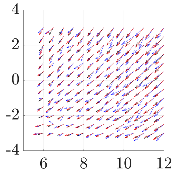
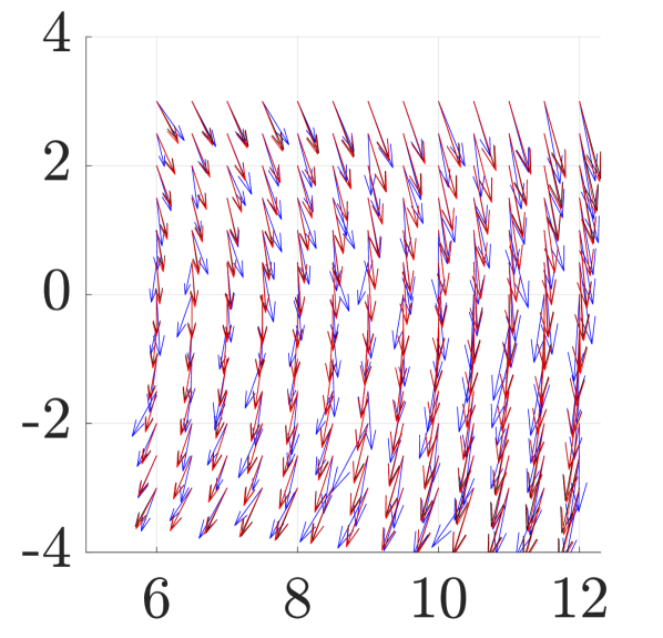
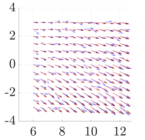
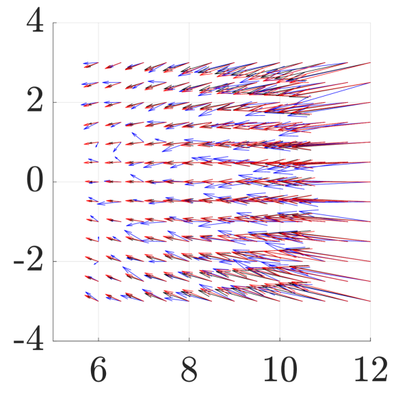
Figure 1: Denoising - noisy, clean, and restored samples are depicted in blue, black, and red arrows, respectively. The clean vector fields are given in Eq. 15 and Eq. 16, in top left complex eigenvalues, top right imaginary eigenvalues, bottom left real eigenvalues, and bottom right nonlinear.

Generalization

Now, the settings of this experiment are as follows. The vector fields in Eq. 15 and Eq. 16 are sampled every $dx=1$. From these samples, the algorithm suggested above generalizes the samples in the domain $[6,12]\times[-3,3]$. In Fig. 2 the sparse samples are blue arrows, the black arrows represent the vector field, and the red ones are the generalized vector field.

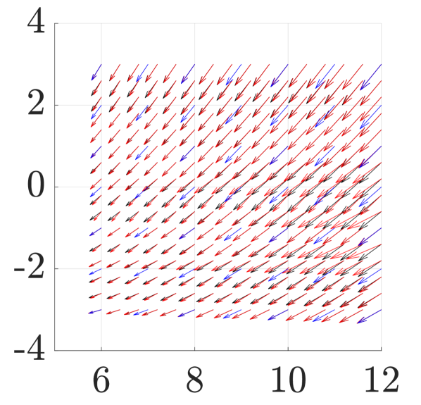
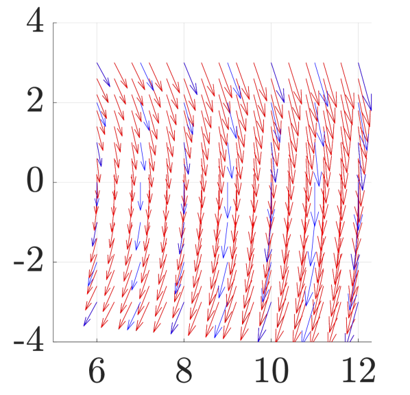
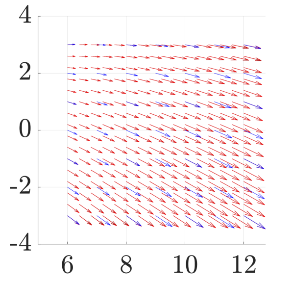
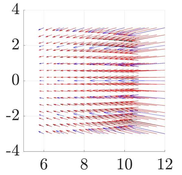
Figure 2: Generalization - blue, black, red arrows are the sparse, original, and generalized samples, respectively. The vector fields are given in Eq. 15 and Eq. 16 where in top left complex eigenvalues, top right imaginary eigenvalues, bottom left real eigenvalues, bottom right is the nonlinear dynamical system.

Dimensionality Reduction

In this toy example, the Lorenz butterfly is considered. Given the dynamical system

$$\begin{split}\dot{x}&=-\sigma x+\sigma y\\ \dot{y}&=\rho x-y-xz\\ \dot{z}&=-\beta z+xy\end{split}$$ (17)

where $\sigma=10,\,\beta=8/3,\,\rho=28$ and initialized with $(1,1,1)^{T}$, the solution is depicted in Fig. 3 (top left). In that solution, the examined vector field is isolated to the red notation. One can see that the dynamic is on a plane in this part. Thus, in this neighborhood, the vector field can be restored with only two Koopman eigenfunctions, i.e. in the optimization problem Eq. 12 $K=2$.

In Fig. 3 top right, one can see the result of the addend $A$ in Eq. 12. The blue and red graphs are the results of $\nabla^{T}m_{i}(\bm{x})P(\bm{x})$. The results are very close to one. Left bottom in Fig. 3 is the result of addend $B$ in Eq. 12, meaning $\nabla m_{1}(\bm{x})$ and $\nabla m_{2}(\bm{x})$ are perpendicular.

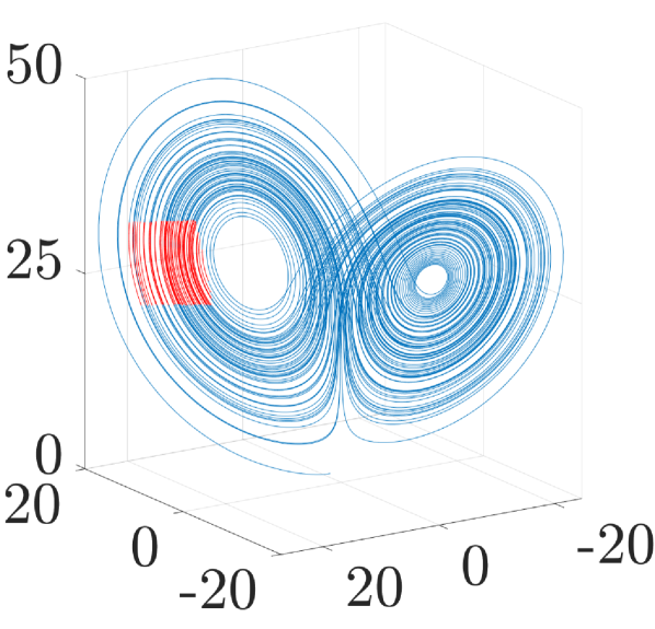
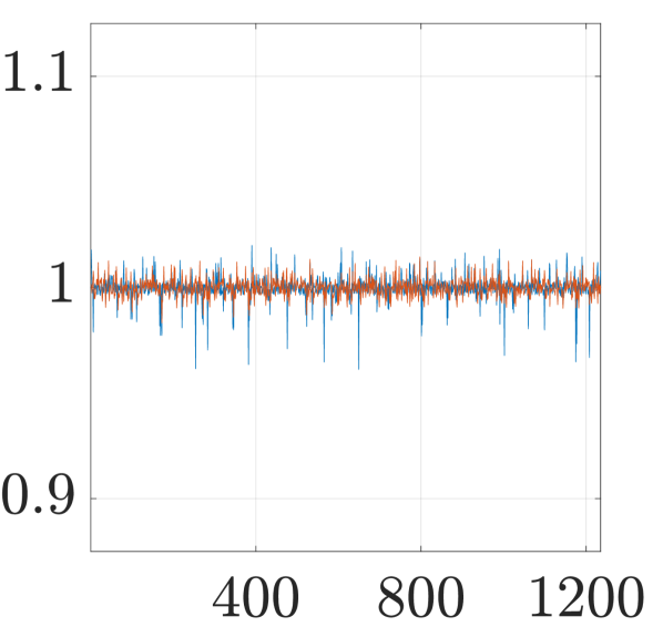
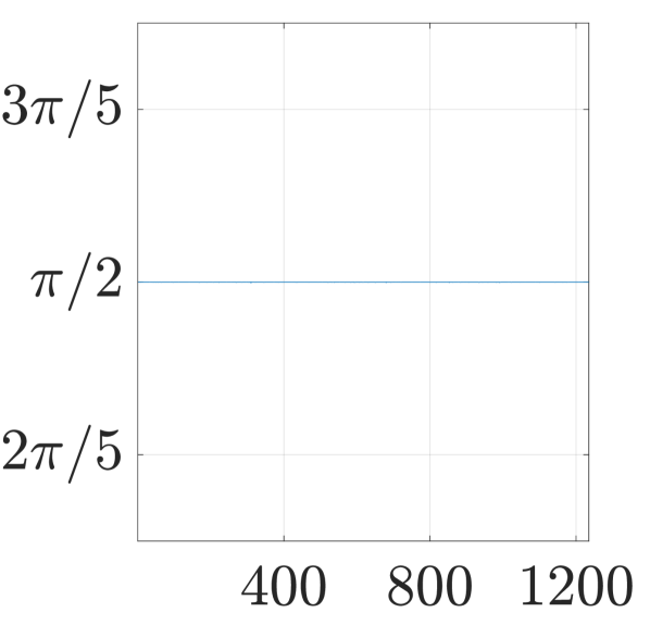
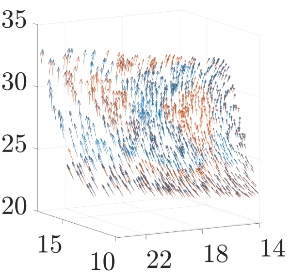
Figure 3: Dimensionality Reduction - top row, left, Lorentz butterfly, the red part approximated as a two dimensional dynamic; right, inner product of the two unit velocity measurements and the vector field; bottom row, left orthogonality of $\nabla m_{1}(\bm{x})$ and $\nabla m_{2}(\bm{x})$ (pointwise), right, vector field restoration, the original (blue) and the restored (red)

IV-D Result Quality

Denoising

In the mentioned above experiments, the noise reduction is about $60\%$ and above. In particular, the noise reduction in the linear system with imaginary eigenfunctions is more than $81\%$. Fig. 4 summarizes the result in this case. In the top left graph of $m_{1}(\bm{x})$ and $m_{2}(\bm{x})$ is given. In the top right, the contours of these manifolds are depicted. In addition, in the bottom row, the histograms of the noise before and after the noise reduction are given.

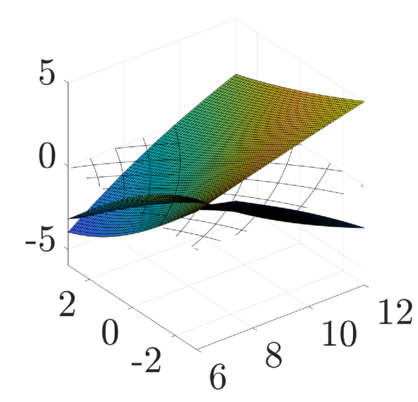
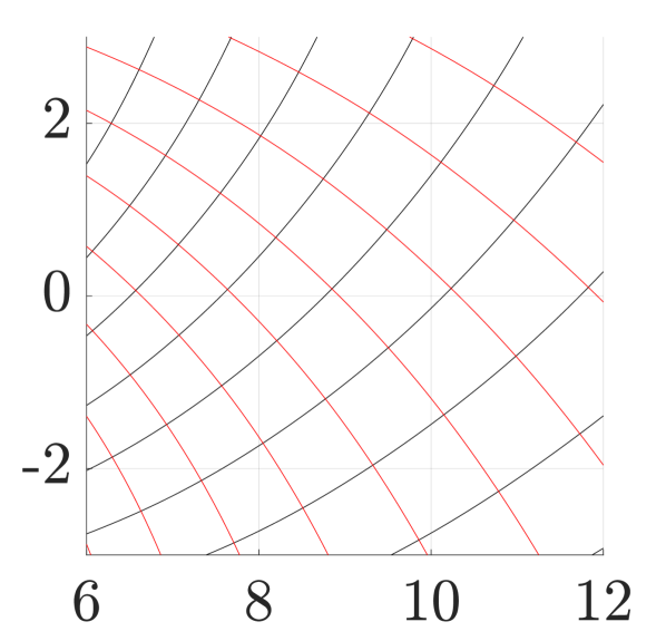
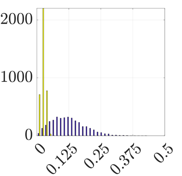
Figure 4: Denoising Quality - Top row, left, unit manifolds, right, contours, bottom row noise histograms before and after Koopman Regularization

Generalization

The generalization process yields accurate results. The error (MSE) in the nonlinear dynamics is $3.01\%$ and in the linear cases for complex eigenvalues $8.45\%$ imaginary $0.25\%$ and real $0.6\%$.

Dimensionality Reduction

The MSE in the experiment of the dimensionality reduction process is $2.5\%$.

V Conclusions

The inherent geometry of a dynamical system is crucial information to restore samples and vector fields. This work shows a way to recover this geometry to restore, generalize, and find a concise representation of vector field samples. The geometry is recovered straightforwardly from the Koopman eigenfunctions and the functionally independent of the minimal set. Thus, this representation seems to be the most concise but accurate one can derive from Koopman eigenfunctions space.

Acronym List

KEF

Koopman Eigenfunction

PDE

Partial Differential Equation

KPDE

Koopman Partial Differential Equation

DMD

Dynamic Mode Decomposition

The Gateaux derivative of a functional $F(u)$ is defined by

$$\partial F/\partial u=\lim_{t\to 0}\frac{F(u+tv)-F(u)}{t}$$ (18)

where $v$ is a test function. The Gateaux derivative of $L(\bm{m})$ with respect to $m_{1}$ can be calculated as the derivatives of addend $A$ and $B$ separately.

Gateaux derivative of $L_{A}$

$$\begin{split}&\partial L_{A}/\partial m_{1}=\lim_{t\to 0}\frac{1}{2t}\int\biggl{[}\left(\nabla^{T}\left(m_{1}(\bm{x})+tv\right)P(\bm{x})-1\right)^{2}\\ &+\sum_{i=2}^{N}\left(\nabla^{T}m_{i}(\bm{x})P(\bm{x})-1\right)^{2}\\ &-\sum_{i=1}^{N}\left(\nabla^{T}m_{i}(\bm{x})P(\bm{x})-1\right)^{2}\biggr{]}d\bm{x}\\ &=\lim_{t\to 0}\frac{1}{2t}\int\biggl{[}\left(\nabla^{T}\left(m_{1}(\bm{x})+tv\right)P(\bm{x})-1\right)^{2}\\ &-\left(\nabla^{T}m_{1}(\bm{x})P(\bm{x})-1\right)^{2}\biggr{]}d\bm{x}\\ &=\int\left(\nabla^{T}m_{1}(\bm{x})P(\bm{x})-1\right)\left(\nabla^{T}vP(\bm{x})\right)d\bm{x}\\ &=-\int v\nabla\cdot\biggl{\{}P(\bm{x})\left(\nabla^{T}m_{1}(\bm{x})P(\bm{x})-1\right)\biggr{\}}d\bm{x}\end{split}$$ (19)

Gateaux derivative of $L_{B}$

$$\begin{split}&\partial L_{B}/\partial m_{1}=\lim_{t\to 0}\frac{1}{2t}\int\biggl{[}\sum_{j=2}^{N}\frac{\left(\nabla^{T}(m_{1}(\bm{x})+tv)\nabla m_{j}(\bm{x})\right)^{2}}{\norm{\nabla m_{1}(\bm{x})+tv}^{2}\norm{\nabla m_{j}(\bm{x})}^{2}}\\ &+\sum_{i=2}^{N}\sum_{j=i+1}^{N}\frac{\left(\nabla^{T}m_{i}(\bm{x})\nabla m_{j}(\bm{x})\right)^{2}}{\norm{\nabla m_{i}(\bm{x})}^{2}\norm{\nabla m_{j}(\bm{x})}^{2}}\\ &-\sum_{i=1}^{N}\sum_{j=i+1}^{N}\frac{\left(\nabla^{T}m_{i}(\bm{x})\nabla m_{j}(\bm{x})\right)^{2}}{\norm{\nabla m_{i}(\bm{x})}^{2}\norm{\nabla m_{j}(\bm{x})}^{2}}\biggr{]}d\bm{x}\\ &=\lim_{t\to 0}\frac{1}{2t}\int\biggl{[}\sum_{j=2}^{N}\frac{\left(\nabla^{T}(m_{1}(\bm{x})+tv)\nabla m_{j}(\bm{x})\right)^{2}}{\norm{\nabla m_{1}(\bm{x})+tv}^{2}\norm{\nabla m_{j}(\bm{x})}^{2}}\\ &-\frac{\left(\nabla^{T}m_{1}(\bm{x})\nabla m_{j}(\bm{x})\right)^{2}}{\norm{\nabla m_{i}(\bm{x})}^{2}\norm{\nabla m_{j}(\bm{x})}^{2}}\biggr{]}d\bm{x}\\ &=\int\sum_{j=2}^{N}\frac{1}{\norm{\nabla m_{j}(\bm{x})}^{2}}\\ &\lim_{t\to 0}\frac{1}{2t}\biggl{[}\frac{\left(\nabla^{T}(m_{1}(\bm{x})+tv)\nabla m_{j}(\bm{x})\right)^{2}}{\norm{\nabla m_{1}(\bm{x})+tv}^{2}}\\ &-\frac{\left(\nabla^{T}m_{1}(\bm{x})\nabla m_{j}(\bm{x})\right)^{2}}{\norm{\nabla m_{1}(\bm{x})}^{2}}\biggr{]}d\bm{x}.\end{split}$$ (20)

The expression in the limit is

$$\begin{split}&=\frac{\left(\nabla^{T}(m_{1}(\bm{x})+tv)\nabla m_{j}(\bm{x})\right)^{2}\norm{\nabla m_{1}(\bm{x})}^{2}}{\norm{\nabla m_{1}(\bm{x})+tv}^{2}\norm{\nabla m_{1}(\bm{x})}^{2}}\\ &-\frac{\left(\nabla^{T}m_{1}(\bm{x})\nabla m_{j}(\bm{x})\right)^{2}\norm{\nabla m_{1}(\bm{x})+tv}^{2}}{\norm{\nabla m_{1}(\bm{x})+tv}^{2}\norm{\nabla m_{1}(\bm{x})}^{2}}.\end{split}$$ (21)

The nominator of this fraction when neglecting $t^{2}$ is

$$\begin{split}&\left(\nabla^{T}(m_{1}(\bm{x})+tv)\nabla m_{j}(\bm{x})\right)^{2}\norm{\nabla m_{1}(\bm{x})}^{2}\\ &-\left(\nabla^{T}m_{1}(\bm{x})\nabla m_{j}(\bm{x})\right)^{2}\norm{\nabla m_{1}(\bm{x})+tv}^{2}\\ &\approx\left(\nabla^{T}m_{1}\nabla m_{j}(\bm{x})+t\nabla^{T}v\nabla m_{j}(\bm{x})\right)^{2}\norm{\nabla m_{1}(\bm{x})}^{2}-\\ &\left(\nabla^{T}m_{1}(\bm{x})\nabla m_{j}(\bm{x})\right)^{2}(\norm{\nabla m_{1}(\bm{x})}^{2}+2t\nabla^{T}m_{1}\nabla v)\\ &\approx\biggl{[}\left(\nabla^{T}m_{1}\nabla m_{j}(\bm{x})\right)^{2}\\ &+2t\left(\nabla^{T}m_{1}\nabla m_{j}(\bm{x})\right)\nabla^{T}v\nabla m_{j}(\bm{x})\biggr{]}\norm{\nabla m_{1}(\bm{x})}^{2}\\ &-\left(\nabla^{T}m_{1}(\bm{x})\nabla m_{j}(\bm{x})\right)^{2}(\norm{\nabla m_{1}(\bm{x})}^{2}+2t\nabla^{T}m_{1}\nabla v)\\ &=2t\nabla^{T}v\nabla m_{j}(\bm{x})\left(\nabla^{T}m_{1}\nabla m_{j}(\bm{x})\right)\norm{\nabla m_{1}(\bm{x})}^{2}\\ &-2t\nabla^{T}m_{1}\nabla v\left(\nabla^{T}m_{1}(\bm{x})\nabla m_{j}(\bm{x})\right)^{2}\\ &=2t\nabla^{T}v\biggl{[}\nabla m_{j}(\bm{x})\norm{\nabla m_{1}(\bm{x})}^{2}\\ &-\nabla m_{1}(\bm{x})\left(\nabla^{T}m_{1}(\bm{x})\nabla m_{j}(\bm{x})\right)\biggr{]}\left(\nabla^{T}m_{1}(\bm{x})\nabla m_{j}(\bm{x})\right).\end{split}$$ (22)

Substituting it back in Eq. 21 and then in Eq. 20 yields

$$\begin{split}&\partial L_{B}/\partial m_{1}\\ &=\int\sum_{j=2}^{N}\frac{1}{\norm{\nabla m_{j}(\bm{x})}^{2}}\nabla^{T}v\biggl{[}\nabla m_{j}(\bm{x})\norm{\nabla m_{1}(\bm{x})}^{2}\\ &-\nabla m_{1}(\bm{x})\left(\nabla^{T}m_{1}(\bm{x})\nabla m_{j}(\bm{x})\right)\biggr{]}\cdot\\ &\frac{\nabla^{T}m_{1}(\bm{x})\nabla m_{j}(\bm{x})}{\norm{\nabla m_{1}(\bm{x})}^{2}\norm{\nabla m_{1}(\bm{x})}^{2}}d\bm{x}\\ &=-\int v\nabla\cdot\biggl{\{}\sum_{j=2}^{N}\biggl{[}\frac{\nabla m_{j}(\bm{x})}{\norm{\nabla m_{j}(\bm{x})}}-\frac{\nabla m_{1}(\bm{x})}{\norm{\nabla m_{1}(\bm{x})}}\\ &\quad\cos\theta_{1,j}\biggr{]}\cdot\frac{\cos\theta_{1,j}}{\norm{\nabla m_{1}(\bm{x})}}\biggr{\}}d\bm{x}\\ \end{split}$$ (23)

where $\cos\theta_{1,j}=\frac{\nabla^{T}m_{1}(\bm{x})\nabla m_{j}(\bm{x})}{\norm{\nabla m_{1}(\bm{x})}\norm{\nabla m_{1}(\bm{x})}}$.