HourglassNeRF: Casting an Hourglass as a Bundle of Rays for Few-shot Neural Rendering

Abstract

Recent advancements in the Neural Radiance Field (NeRF) have bolstered its capabilities for novel view synthesis, yet its reliance on dense multi-view training images poses a practical challenge. Addressing this, we propose HourglassNeRF, an effective regularization-based approach with a novel hourglass casting strategy. Our proposed hourglass is conceptualized as a bundle of additional rays within the area between the original input ray and its corresponding reflection ray, by featurizing the conical frustum via Integrated Positional Encoding (IPE). This design expands the coverage of unseen views and enables an adaptive high-frequency regularization based on target pixel photo-consistency. Furthermore, we propose luminance consistency regularization based on the Lambertian assumption, which is known to be effective for training a set of augmented rays under the few-shot setting. Leveraging the inherent property of a Lambertian surface, which retains consistent luminance irrespective of the viewing angle, we assume our proposed hourglass as a collection of flipped diffuse reflection rays and enhance the luminance consistency between the original input ray and its corresponding hourglass, resulting in more physically grounded training framework and performance improvement. Our HourglassNeRF outperforms its baseline and achieves competitive results on multiple benchmarks with sharply rendered fine details. The code will be available.

1 Introduction

In recent years, the Neural Radiance Field (NeRF) [24] has emerged as a dominant paradigm in the domain of novel view synthesis, owing to its outstanding capability to produce high-quality rendered images and its inherently simplistic architectural design. Numerous advancements have been introduced to the NeRF [20, 3, 21, 23, 12, 43, 19, 18], propelling its performance to greater heights. However, its dependency on a dense set of multi-view training images still exists as a critical challenge for practical application.

In the realm of few-shot novel view synthesis, two primary approaches have emerged as mainstream methodologies: pre-training and regularization. The pre-training methods [4, 5, 41, 22, 10, 17, 31, 38, 13, 46] necessitate extensive datasets comprising diverse scenes captured from multiple viewpoints, facilitating the infusion of prior knowledge for 3D geometry during the pre-training phase. However, it is highly expensive to collect large-scale datasets necessary for pre-training.

Mip-NeRF [1]

RegNeRF [25]

FlipNeRF [33]

FreeNeRF [45]

HourglassNeRF

Ground Truth

Figure 1: Comparison with other baselines. Our HourglassNeRF achieves superior quality of fine details and textures to other state-of-the-art methods by applying the hourglass casting strategy equipped with an adaptive high-frequency regularization. The last two rows of the figure indicate the types of ray augmentation schemes and frequency regularization methods, respectively.

In contrast, the regularization methods [25, 34, 14, 9, 32, 6, 16, 33, 45, 39, 35] are optimized to individual scenes, harnessing supplementary training assets, such as rays generated from unseen views [33, 25, 14, 16], pseudo-depth maps [6, 32, 39], readily available off-the-shelf models [9, 25], and so on. Moreover, these methods may directly introduce regularization techniques to the internal components of a NeRF framework, e.g. the density outputs of ray samples [34], the high-frequency segments stemming from positional encoding [45, 35], and so on. Although these methods have achieved promising results, they often rely on additional training resources, which may not be consistently accessible. Additionally, the existing frequency regularization technique requires the range of visible spectrum and the duration of masking phase, both of which should be set manually.

Inspired by prior works [33, 45], we propose HourglassNeRF, which utilizes a novel hourglass casting strategy as an effective ray augmentation scheme. We cast an hourglass as a bundle of multiple additional rays, by featurizing the 3D Gaussian space of conical frustum using the Integrated Positional Encoding (IPE) [1]. This allows us to cover a broader area of unseen views as an additional training resource, further enhancing the efficiency of augmented rays. Furthermore, by applying IPE to the hourglass, we can adaptively apply high-frequency regularization based on the photo-consistency of the pixels where the original input ray and the newly generated hourglass are cast. It allows us to eliminate the hand-crafted aspects of the existing frequency regularization scheme and capture fine details better while preventing from overfitting to the high-frequency.

Our proposed HourglassNeRF is built upon FlipNeRF [33], which trains a set of augmented rays with existing ground-truth (GT) pixel values by taking advantage of Lambertian assumption. However, despite the Lambertian surface assumption, FlipNeRF utilized a set of flipped specular reflection rays, which goes against the physical characteristics of the training framework. Instead, we assume our proposed hourglass as a featurized bundle of flipped diffuse reflection rays originating from Lambertian surfaces, enabling a more physically reasonable training framework and leading to performance improvement. Furthermore, building upon the characteristic that a Lambertian surface maintains consistent luminance regardless of the viewing angle, we introduce luminance consistency regularization with an auxiliary luminance estimation task to enhance the consistency of estimated luminances between the original ray and its corresponding hourglass, which further improves the rendering quality as shown in Fig. 1. Our main contributions are summarized as follows:

• We propose a novel ray augmentation strategy, i.e. casting an hourglass as a bundle of additional rays, which is effective for training NeRF with only a set of sparse inputs.

• By marrying the IPE with our proposed hourglass, we can adaptively regularize the high-frequency of additional input samples based on the photo-consistency, which leads to performance improvement under the few-shot setting.

• Furthermore, inspired by the fact that the Lambertian surface has the consistent luminance irrespective of viewing angle, we assume our proposed hourglass as multiple flipped diffuse reflection rays cast back from the Lambertian surface, and propose luminance consistency regularization for training our HourglassNeRF. By enhancing the consistency of estimated relative luminances between the original ray and the corresponding hourglass, we can further improve the integrity of our training framework and the rendering quality.

• Our HourglassNeRF outperforms its baseline, delivering competitive results across different datasets and scenarios with sharp fine details.

2 Related Works

2.1 Neural Radiance Fields

The advent of NeRF [24] has facilitated a paradigm shift in novel view synthesis, achieving remarkable rendering quality. The NeRF employs a Multilayer Perceptron (MLP) to represent a scene, correlating spatial coordinates and viewing directions with corresponding color and volumetric density attributes, and then generates a novel view by volume rendering techniques. While NeRF’s versatility has been demonstrated across a gamut of applications—from the 3D object generation [20, 26, 21, 23] to capturing human performances [44, 48, 36, 12, 43], and even extending to dynamic videos [7, 19, 18, 37, 29]—its efficacy is notably hindered by a fundamental constraint: the reliance on a dense set of training images. This requirement poses significant challenges, particularly in scenarios restricted to a scant number of views, thus hampering its practical application. In addressing this critical bottleneck, our work focuses on improving NeRF’s performance under the constraints of limited input.

2.2 Few-shot Neural Rendering

In the emerging field of few-shot novel view synthesis, two principal strategies are prevalent: pre-training and regularization. The pre-training methods [4, 5, 41, 22, 10, 17, 31, 38, 13, 46] rely on large-scale datasets of multi-view scenes to infuse a NeRF model with a 3D geometry prior, often followed by fine-tuning on specific target scenes. In contrast, the regularization methods [25, 34, 14, 9, 32, 6, 16, 33, 45, 39, 35] are optimized to individual scenes by leveraging auxiliary training aids, e.g. pseudo-depth maps [6, 32, 39], augmented training rays [33, 25, 14, 16], semantic consistencies [9], and so on for additional guidance.

A notable technique within this approach, FlipNeRF [33], assumes the objects’ surface as Lambertian, which is effective in training extra data for few-shot NeRF, and exploits flipped specular reflection rays as additional training data, yielding promising outcomes. However, since Lambertian surfaces primarily exhibit diffuse reflection, using specular reflections goes against the physical traits expected under Lambertian assumptions, posing a challenge to the training framework’s integrity.

Recently, the studies tackling the issue of overfitting to high-frequency in the few-shot scenario [45, 35] have emerged. FreeNeRF [45] pioneered a frequency regularization approach to adjust the visible frequency range based on the training time steps. Despite its meaningful observation and promising results, it requires a manually designed masking phase and strong prior specific to a dataset, showing a lack of fine details depending on the scenes’ structures due to the heuristically regulated high-frequency.

In this work, we propose a novel hourglass casting strategy, which utilizes a featurized bundle of flipped diffuse reflection rays that conform to the physical expectations of Lambertian surfaces within our training framework. Furthermore, by applying IPE to featurize the hourglass, we can regulate the high-frequency of the additional hourglass adaptively based on the target pixel photo-consistency between the original input ray and the corresponding hourglass, leading to the improved rendering quality with clear fine details.

2.3 Ray Parameterization of NeRF

Since the original NeRF casts an infinitesimally narrow ray with point sampling, there has been a line of research exploring the effective ray shapes for higher-quality rendering, i.e. method to parameterize the ray [40, 1, 2, 8]. Among them, mip-NeRF [1] proposed a cone tracing strategy, in which each conical frustum area of the samples is featurized by the IPE, to tackle the aliasing problem. Mip-NeRF 360 [2] utilized contracted scene representation, which is an extended version of the mip-NeRF’s parameterization to unbounded scenes. Recently, Exact-NeRF [8] introduced a pyramidal parameterization method by using an analytically precise encoding technique instead of the IPE’s 3D Gaussian approximation, leading to performance improvement for unbounded scenes. In this paper, we propose a novel hourglass casting strategy as an effective ray augmentation scheme for few-shot NeRF, which we conceptualize as a featurized bundle of multiple rays, enabling an adaptive frequency regularization by combining with IPE. To the best of our knowledge, our HourglassNeRF is the first attempt to tackle the few-shot novel view synthesis task through the lens of ray parameterization.

3 Methods

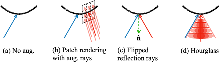
Figure 2: Comparative overview of ray augmentation techniques. In contrast to other augmentation strategies ((b), (c)), where each additional ray corresponds to a single unseen view, our hourglass (d) encompasses a wider area of unseen views, thereby boosting the augmentation’s efficacy. Technically, the rays are spanned over the object surface as used in the typical NeRF’s volume rendering technique, but we simplify the illustration for easy comparison between the methods. Kindly refer to Fig. 3 for a more detailed description. The blue and red rays indicate the original and augmented ray, respectively.

In this work, we propose HourglassNeRF, an effective regularization method for few-shot novel view synthesis with an hourglass casting strategy. Our HourglassNeRF is built upon FlipNeRF, which utilizes flipped reflection rays with Lambertian assumption (Sec. 3.1). We generate a set of hourglasses whose conical frustums are featurized by IPE and cast them toward the identical target pixels as additional training rays, adaptively regulating their high-frequency components (Sec. 3.2). Furthermore, taking advantage of the characteristics of the Lambertian assumption, we propose the luminance consistency regularization to enhance the consistency of the estimated relative luminances between the original ray and its corresponding hourglass, leading to further performance improvement (Sec. 3.3). A brief comparison with different ray augmentation schemes is shown in Fig. 2.

3.1 Preliminaries

Mip-NeRF.

The mip-NeRF [1], which casts cones instead of rays to alleviate aliasing, represents a 3D scene by mapping 3D coordinates $\mathbf{x}=(x,y,z)$ and viewing directions $(\theta,\phi)$ to the colors $\mathbf{c}=(r,g,b)$ and volumetric densities $\tau$:

$$f(\gamma^{*}(\mathbf{x}),\gamma(\mathbf{d}))\to(\mathbf{c},\tau),$$ (1)

where $f(\cdot,\cdot)$, $\gamma(\cdot)$, $\gamma^{*}(\cdot)$ and $\mathbf{d}$ denote an MLP-based network, original positional encoding, IPE, and 3D Cartesian unit vector practically used as an input viewing direction, respectively. Compared to the original NeRF which utilizes point-sampling, mip-NeRF featurizes the conical frustum area $\mathrm{F}(\mathbf{d},\mathbf{o},\dot{\rho},t_{i},t_{i+1})$ by an approximated IPE, where $\mathbf{o}$ and $\dot{\rho}$ indicate the camera origin and base radius of a cone, respectively:

$$\begin{split}\gamma^{*}&(\mathbf{x})=\gamma^{*}(\boldsymbol{\mu},\boldsymbol{\Sigma})=\mathbb{E}_{x\sim\mathcal{N}(\mathbf{P}\boldsymbol{\mu},\mathbf{P}\mathbf{\Sigma}\mathbf{P}^{\top})}\left[\gamma(\mathbf{x})\right]\\ &=\begin{bmatrix}\sin(\mathbf{P}\boldsymbol{\mu})\circ\exp(-0.5\text{diag}(\mathbf{P}\mathbf{\Sigma}\mathbf{P}^{\top}))\\ \cos(\mathbf{P}\boldsymbol{\mu})\circ\exp(-0.5\text{diag}(\mathbf{P}\mathbf{\Sigma}\mathbf{P}^{\top}))\end{bmatrix}\,.\end{split}$$ (2)

Here, $\boldsymbol{\mu}$, $\boldsymbol{\Sigma}$, $\mathbf{P}$, and $\circ$ denote the mean and covariance of the conical frustum approximated with multivariate Gaussians, the positional encoding basis matrix, and the element-wise multiplication, respectively. We kindly refer to [1] for more technical details.

Then each target pixel is rendered by alpha compositing the output colors and densities along the input cone $\mathbf{r}(t)=\mathbf{o}+t\mathbf{\bar{d}}$, where $\mathbf{\bar{d}}=\lVert\mathbf{\bar{d}}\rVert_{2}\cdot\mathbf{d}$. In practice, the volume rendering integrals are approximated using a quadrature rule [24] as follows:

$$\mathbf{\hat{c}(r)}=\sum_{i=1}^{N}w_{i}\mathbf{c}_{i}=\sum_{i=1}^{N}T_{i}(1-\exp(-\tau_{i}\delta_{i}))\mathbf{c}_{i},$$ (3)

where $T_{i}=\exp(-\sum_{j=1}^{i-1}\tau_{j}\delta_{j})$. Note that $w_{i}$, $\delta_{i}$ and $N$ indicate the alpha blending weight, the interval between adjacent samples and the number of samples, respectively. Finally, the radiance field is trained by minimizing the mean squared errors (MSE) between the rendered pixels and GTs:

$$\mathcal{L}_{\text{MSE}}=\sum_{\mathbf{r}\in\mathcal{R}}||\mathbf{\hat{c}(r)}-\mathbf{c_{\text{GT}}(r)}||^{2}_{2}\,,$$ (4)

where $\mathcal{R}$ is a batch of inputs.

FlipNeRF.

Implemented upon mip-NeRF, the FlipNeRF [33] utilizes a set of flipped reflection rays $\mathbf{r}^{\prime}$ as additional training rays, which are derived from the original ray directions $\mathbf{\bar{d}}$ and the estimated normal vectors $\mathbf{\hat{n}}=\sum_{i=1}^{N}w_{i}\mathbf{n}_{i}$ as follows:

$$\mathbf{r}^{\prime}(t)=\mathbf{o}^{\prime}+t\mathbf{d}^{\prime},$$ (5)

where $\mathbf{d}^{\prime}=2(\mathbf{\bar{d}}\cdot\hat{\mathbf{n}})\hat{\mathbf{n}}-\mathbf{\bar{d}}$ and $\mathbf{o}^{\prime}=\mathbf{p}_{s}-t_{s}\mathbf{d}^{\prime}$ indicate the flipped reflection direction and the newly set camera origin derived from the object’s estimated surface $\mathbf{p}_{s}=\mathbf{o}+t_{s}\mathbf{\bar{d}}$, respectively. Note that $t_{s}$ is the distance to the estimated object surface. Taking advantage of Lambertian surface assumption, which is useful for a few-shot training framework utilizing the GT pixel values of original rays to provide relevant supervisory signals for additional rays, the flipped reflection rays can be optimized effectively with filtering the ineffective rays whose angle with the corresponding original rays are over the masking threshold $\psi=90^{\circ}$. However, despite the Lambertian assumption, the FlipNeRF makes use of specular reflection rays, which are mainly originated from the non-Lambertian surface, making its framework conflict with physical characteristics.

Our HourglassNeRF is built upon FlipNeRF while achieving better rendering quality with more fine details compared to FlipNeRF thanks to our proposed hourglass casting. Furthermore, we conceptualize the hourglass as a bundle of flipped diffuse reflection rays in line with the Lambertian assumption, leading to a more physically reasonable training framework.

3.2 Hourglass Casting

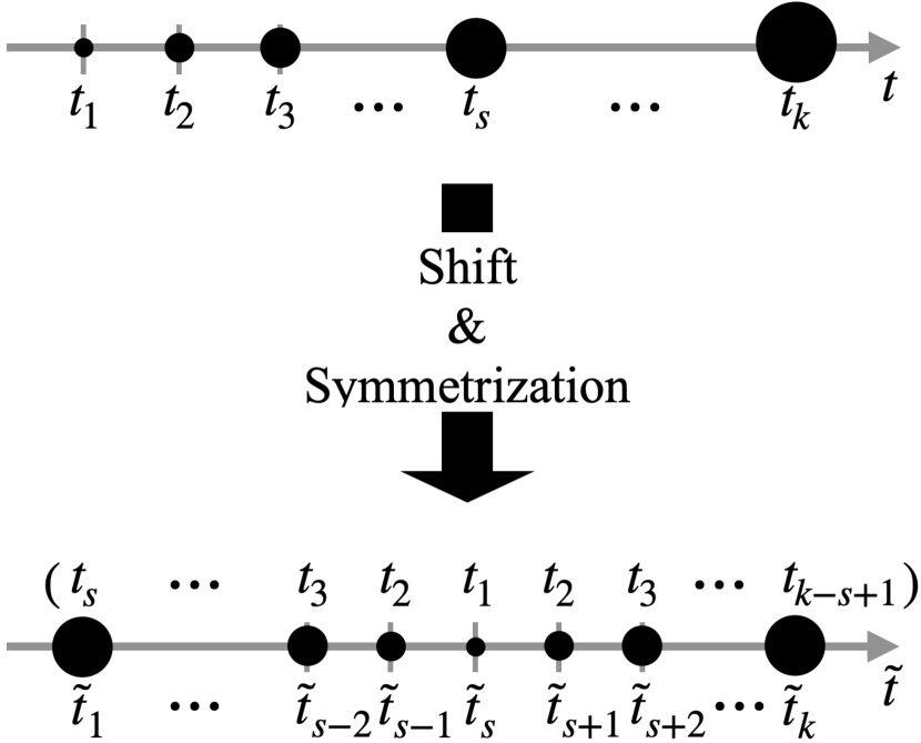
(a) Metric distance reparameterization

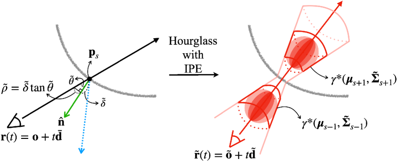
(b) Hourglass featurization by IPE

Figure 3: Hourglass generation process. (a) First, to derive $\tilde{\sigma}^{2}_{\rho}$, we reparameterize the original metric distance $t$ as $\tilde{t}$. We shift $t_{1}$, i.e. starting point of a ray along a z-axis, to the estimated object surface $\mathbf{p}_{s}$, so that our proposed hourglass is symmetrically constructed around $\mathbf{p}_{s}$, i.e. $\tilde{t}_{s-i}=\tilde{t}_{s+i}$ and it leads to $\boldsymbol{\tilde{\Sigma}}_{s-i}=\boldsymbol{\tilde{\Sigma}}_{s+i}$. Note that $\tilde{t}$ is used only for $\tilde{\sigma}^{2}_{\rho}$. (b) Using the trigonometric function, we compute the base radius of hourglass $\tilde{\rho}$. As a result, our proposed hourglass $\mathbf{\tilde{r}}$ is featurized to cover the unseen view area between the original ray and its reflection ray. The blue dotted ray denotes the reflection ray of $\mathbf{r}$.

We propose an hourglass-shaped ray as an effective additional training ray for few-shot NeRF. As shown in Fig. 2, compared to the existing ray augmentation schemes where a resulting augmented ray corresponds to an unseen view, our proposed hourglass covers the area of continuous unseen views by IPE presented in Eq. 2, providng more efficient extra training resources.

First, as demonstrated in Fig. 3(a), we reparameterize the metric distance $t\in[t_{near},$ $t_{far}]$ as $\tilde{t}$ to derive the variance $\tilde{\sigma}^{2}_{\rho}$, which is perpendicular to the hourglass. We shift $t$ so that the value of starting point $t_{1}$ is located on the distance to the estimated object surface $t_{s}$, resulting in $\tilde{t}_{s}=t_{1}$. And then we set $[t_{1},t_{s-1}]$ values to be symmetric with respect to $t_{s}$.

Next, as shown in Fig. 3(b), we derive a base radius of the hourglass $\tilde{\rho}$ from the angle $\tilde{\theta}$ between $\mathbf{r}$ and $\mathbf{\hat{n}}$ using the trigonometric function as follows:

$$\tilde{\rho}=\tilde{\delta}\tan{\tilde{\theta}},$$ (6)

where $\tilde{\delta}=1-\tilde{t}_{s}$ so that $\tilde{\rho}$ is obtained from the sample located on $\tilde{t}=1$ following [1]. However, directly employing the obtained $\tilde{\rho}$ in IPE results in significantly large $\tilde{\sigma}^{2}_{\rho}$, leading to over-regularization of high-frequency components for the samples along an hourglass. Thus, we adjust the scale of $\tilde{\rho}$ to $[0,1]$ to contract $\tilde{\rho}$ with the large $\tilde{\theta}$ value into a proper range, while leaving the one with small $\tilde{\theta}$ affected little as follows:

$$\tilde{\rho}=\exp{(-1/(\tilde{\delta}\tan{\tilde{\theta}}))}.$$ (7)

This ensures high-frequency regularization is appropriately applied.

And then, $\tilde{\sigma}^{2}_{\rho}$ is derived from $\tilde{t}$ and $\tilde{\rho}$ to featurize the conical frustums of hourglass as multivariate Gaussian by simply replacing the original metric distance $t$, which is used in mip-NeRF, with $\tilde{t}$ as follows:

$$\tilde{\sigma}^{2}_{\rho}=\tilde{\rho}^{2}\left(\frac{\tilde{t}^{2}_{\mu}}{4}+\frac{5\tilde{t}^{2}_{\delta}}{12}-\frac{4\tilde{t}^{4}_{\delta}}{15(3\tilde{t}^{2}_{\mu}+\tilde{t}^{2}_{\delta})}\right),$$ (8)

where $\tilde{t}_{\delta}$ and $\tilde{t}_{\mu}$ denote a half-width and mid-point of adjacent $\tilde{t}$ values. Note that we use the same $\mu_{t}$ and $\sigma^{2}_{t}$ for the mean and variance along the hourglass as mip-NeRF.

Finally, we generate an hourglass $\mathbf{\tilde{r}}(t)=\mathbf{\tilde{o}}+t\mathbf{\tilde{d}}$, where $\mathbf{\tilde{d}}=-\mathbf{\hat{n}}$ and $\mathbf{\tilde{o}}=\mathbf{p}_{s}-t_{s}\mathbf{\tilde{d}}$, so that the hourglass is cast from the newly set camera origin $\mathbf{\tilde{o}}$, which has the same distance from $\mathbf{p}_{s}$ as the original ray, covering the unseen view area between the original ray and the corresponding reflection ray around the axis of $\mathbf{\hat{n}}$. Implemented upon FlipNeRF, our HourglassNeRF is optimized with the same training losses while using our proposed hourglasses as an additional training batch instead of flipped reflection rays.

Since the target pixel photo-consistency between $\mathbf{r}$ and $\mathbf{\tilde{r}}$ varies depending on the angle $\tilde{\theta}$ between them, which is used to derive the base radius of hourglass $\tilde{\rho}$ and the x/y-axis variance $\tilde{\sigma}^{2}_{\rho}$, the high-frequency spectrum of samples along $\mathbf{\tilde{r}}$ are regulated adaptively based on the photo-consistency, i.e. the less photo-consistent the target pixel is, the more regulated the samples’ high-frequency components are. It eliminates the need for manually designing a frequency spectrum to regularize during the training phase and effectively adjusts the amount of high-frequency detail retained in additional training samples for learning fine details.

3.3 Luminance Consistency Regularization

As our proposed hourglass covers an area of continuous unseen views, we conceptualize it as a bundle of multiple flipped diffuse reflection rays originating from the Lambertian surface (Fig. B in supplementary material). Furthermore, leveraging the property of Lambertian surfaces, which maintain constant luminance at a pixel regardless of the viewing angle, we propose a luminance consistency regularization.

For simplicity, we use a relative luminance value, which is normalized as $[0,1]$, and derive the GT relative luminance $y_{\text{GT}}$ of a target pixel as follows:

$$y_{\text{GT}}=\sum_{\bar{c}}^{\{\bar{r},\bar{g},\bar{b}\}}\lambda_{\bar{c}}\bar{c},$$ (9)

where $\bar{c}=c_{\text{GT}}^{2.2}$ indicates a linear rgb component converted from the gamma-compressed one by applying a simple power curve [27]. We set the linear coefficients $\lambda_{\mathbf{\bar{c}}}=\left(\lambda_{\bar{r}},\lambda_{\bar{g}},\lambda_{\bar{b}}\right)$ as $0.2126$, $0.7152$, and $0.0722$, respectively, considering that green light, as the predominant element of luminance, contributes the most to human light perception, with blue light being the least contributing one [30, 28].

In addition to the existing outputs, our HourglassNeRF estimates the luminance $y$ as additional outputs per sample along a ray and renders the final luminance $\hat{y}$ by volume rendering as follows:

$$\hat{y}(\mathbf{r})=\sum_{i=1}^{N}w_{i}y_{i},$$ (10)

where $y_{i}\in[0,1]$ is the estimated relative luminance of the $i$-th sample along a ray $\mathbf{r}$. The estimated luminance map is trained to minimize MSE:

$$l_{\text{lum.}}=\sum_{\mathbf{r}\in\mathcal{R}}||\hat{y}(\mathbf{r})-y_{\text{GT}}(\mathbf{r})||^{2}_{2}.$$ (11)

The luminance map estimated from the hourglass is also optimized using the same $y_{\text{GT}}$ by minimizing the corresponding MSE loss $\tilde{l}_{\text{lum.}}$, resulting in our proposed training loss $\mathcal{L}_{\text{lum.}}=\eta l_{\text{lum.}}+\tilde{\eta}\tilde{l}_{\text{lum.}}$, where $\eta$ and $\tilde{\eta}$ are balancing weights.

By optimizing the volumetric rendered luminance, we can provide extra supervisory signals, whose GT luminances are obtained from GT pixel values without any burdensome process, to the blending weights $w$, which are directly related to the estimated depth map of NeRF. As a result, it leads to performance improvement under the few-shot scenario, and also enables a more physically consistent framework than FlipNeRF, adhering to the Lambertian surface assumption. Further details about the total loss and architecture are provided in the supplementary material.

4 Experiments

4.1 Experimental Details

Datasets and metrics.

We evaluate our HourglassNeRF and other baselines on three representative datasets for novel view synthesis: Realistic Synthetic 360^∘ [24], DTU [11], and Shiny Blender [40]. Realistic Synthetic 360^∘ has 8 synthetic scenes, each containing 400 multi-view images with a white background. We use 4 and 8 views to train our HourglassNeRF, and conduct an analysis of the frequency regularization effect and the effect of luminance estimation within the 4-view setting, using the first 4 and 8 images from the training set for a fair comparison, following the protocol in [34, 33]. On the DTU dataset, featuring multi-view images with objects against a white table and black background, we compare HourglassNeRF against other methods across 3/6/9-view scenarios and perform an ablation study in the 3-view context, following [46]. Furthermore, we evaluate our method on Shiny Blender, which comprises 6 synthetic glossy objects, i.e. objects that are largely non-Lambertian.

For quantitative evaluation, we use the metrics such as PSNR, SSIM [42], LPIPS [47], and the geometric average [1], each averaged across all scenes within each dataset. Note that we use the masked evaluation metrics to avoid the background bias and focus on the target objects.

Baselines.

We compare our HourglassNeRF against the state-of-the-art (SOTA) regularization methods [9, 14, 25, 34, 45, 33] and the original mip-NeRF [1] on Realistic Synthetic 360^∘. We also evaluate against pre-training [4, 5, 46] and regularization methods on the DTU dataset. On Shiny Blender, our HourglassNeRF is compared with FlipNeRF [33] and FreeNeRF [45], designed for ray augmentation and high-frequency regularization, respectively, as well as Ref-NeRF [40] tackling the view-dependent effects of non-Lambertian surfaces. The pre-training methods utilize DTU for pre-training, whereas regularization approaches and mip-NeRF are optimized per scene. Note that we report the results of other methods from [25, 34, 33], which outperformed the results from the corresponding original paper by modified training curriculum [25] and used the same training views to ensure a fair comparison [34, 33]. Kindly refer to our supplementary material for more experimental details.

4.2 Analysis of HourglassNeRF

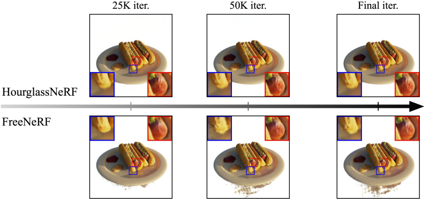
Figure 4: Comparison of fine details against FreeNeRF over the training phase. Compared to FreeNeRF which forcibly masks the high-frequency spectrum in the early training phase, our HourglassNeRF adaptively regularizes the high-frequency components of additional ray samples based on the target pixel photo-consistency (i.e. the angle between the original ray and hourglass) during the whole training process. As a result, our HourglassNeRF already achieves sharper fine details at 25K iteration than the fully trained FreeNeRF.

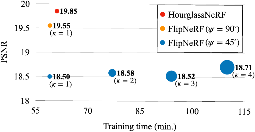
Figure 5: Comparison of our HourglassNeRF against multicasting strategy on DTU 3-view. Our HourglassNeRF outperforms FlipNeRF in all scenarios by a large margin, showing the superior efficiency as a ray augmentation method. The training time per scene is measured using the same GPU, iterations, and batch size. Note that FlipNeRF ($\psi=90^{\circ}$) experiences training instability when $\kappa>1$ due to an excessive number of additional training rays, which are inaccurately estimated during the initial training phase. The size of circles is proportional to $\kappa$, i.e. the number of augmented rays per original ray.

Frequency regularization effect of hourglass.

Fig. 5 demonstrates the comparison between our HourglassNeRF and FreeNeRF, which is specialized for frequency regularization. Our HourglassNeRF renders sharper fine details than FreeNeRF from the earlier training phase and already achieves competitive rendering quality only after 25K training iterations compared to the fully trained FreeNeRF. Although FreeNeRF prevents overfitting by forcibly masking most of high-frequency components during early training, it results in non-satisfactory rendering outcomes that fail to capture fine details in the end. In contrast, our HourglassNeRF adaptively regularizes the high-frequency components of the hourglass samples based on the target pixel photo-consistency, preventing overfitting and enabling sharper rendering.

Effectiveness of hourglass as a bundle of rays.

In Fig. 5, we demonstrate the effectiveness of hourglass, which covers multiple unseen views, compared to FlipNeRF with a different number of augmented rays, i.e. the multicasting strategy. Based on FlipNeRF, we cast $\kappa$ extra rays per original ray $\mathbf{r}$, consisting of flipped reflection ray $\mathbf{r}^{\prime}$ and additional rays which are evenly spaced between $\mathbf{r}$ and its corresponding $\mathbf{r}^{\prime}$, i.e. within the area of our hourglass, toward the same target pixel. Note that we set the masking threshold $\psi=45^{\circ}$ identically for a fair comparison. When $\kappa=1$, which amounts to the vanilla FlipNeRF, our HourglassNeRF outperforms FlipNeRF by a large margin, showing the efficacy of hourglass. However, exploiting $\kappa>1$ augmented rays, fails to achieve meaningful performance improvement. This suggests that our single hourglass casting, equipped with adaptive frequency regularization, is more effective than multicasting strategy over the same unseen area. Moreover, for a training efficiency, simply increasing the number of augmented rays in the multicasting strategy leads to longer training time due to the additional ray processing. However, our HourglassNeRF maintains training efficiency while improving performance by featurizing continuous unseen views with a single hourglass.

RegNeRF [25]

FlipNeRF [33]

FreeNeRF [45]

HourglassNeRF

HourglassNeRF†

Ground Truth

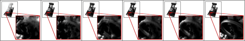
Figure 6: Qualitative results of relative luminance maps. Our HourglassNeRF renders clearer relative luminance map than other baselines. With our explicitly estimated luminance $\hat{y}$, ours^† captures the detailed luminance on the handle more accurately. The red insets are visualized with doubled contrast for ease of comparison.

Table 1: Comparison of relative luminance map. $\dagger$ indicates the explicitly estimated luminance map $\hat{y}$ while others compute lumniance based on estimated RGB values.

	PSNR $\uparrow$	SSIM $\uparrow$	LPIPS $\downarrow$	Average $\downarrow$
RegNeRF [25]	5.71	0.780	0.291	0.368
FlipNeRF [33]	16.49	0.878	0.080	0.092
FreeNeRF [45]	15.63	0.869	0.091	0.113
HourglassNeRF	16.87	0.886	0.074	0.088
HourglassNeRF†	17.18	0.891	0.062	0.079

Table 2: Ablation study. Thanks to the proposed hourglass and $\mathcal{L}_{\text{lum.}}$, our HourglassNeRF achieves superior performance to its baseline FlipNeRF across all metrics.

	Hourglass	$\mathcal{L}_{\text{lum.}}$	PSNR $\uparrow$	SSIM $\uparrow$	LPIPS $\downarrow$	Avg. $\downarrow$
FlipNeRF [33]			19.55	0.767	0.180	0.101
(1)	✓		19.51	0.774	0.147	0.097
(2)		✓	18.44	0.747	0.201	0.119
(3)	✓	✓	19.85	0.773	0.146	0.096

Luminance estimation as an auxiliary task.

We show the quantitative and qualitative results of our proposed luminance estimation in Tab. 2 and Fig. 6, respectively. Since other baselines do not estimate the relative luminance $\hat{y}$ explicitly, their estimated luminance maps $\hat{y}^{\mathbf{c}}$ are derived from the estimated colors using Eq. 9 and we report our results of both $\hat{y}^{\mathbf{c}}$ and $\hat{y}$ for a fair comparison. Ours outperforms other representative methods based on the ray augmentation and frequency regularization. As illustrated in Fig. 6, our HourglassNeRF renders much clearer relative luminance maps than other baselines. Since the resulting relative luminances and pixel values share the identical blending weights $w$ for volumetric rendering, we are able to provide extra supervisory signals to the blending weights and effectively regularize them by the luminance estimation task.

4.3 Ablation Study

Tab. 2 shows the ablation study of our HourglassNeRF. By replacing the flipped reflection rays of FlipNeRF with our hourglass (1), it achieves performance improvement across most of the metrics, especially on SSIM and LPIPS by a large margin. However, it achieves rather degenerate results with only $\mathcal{L}_{\text{lum.}}$ (2). Since the flipped reflection rays are technically based on the specular reflection, our $\mathcal{L}_{\text{lum.}}$ goes against the physical concept of FlipNeRF training framework, leading to the performance drop. When we optimize our HourglassNeRF with our proposed $\mathcal{L}_{\text{lum.}}$ together ((1) $\rightarrow$ (3)), we can further enhance the rendering quality with clear fine details, especially on PSNR metric. Additional experiment of the masking threshold for hourglass is provided in our supplementary material.

4.4 Comparison with other Baselines

Realistic Synthetic 360^∘.

As shown in Tab. 3 and Fig. 7, our HourglassNeRF achieves the SOTA performance over all the scenarios and metrics. Compared to RegNeRF and FlipNeRF, which utilize ray augmentation for training, ours renders superior quality of objects, with better capturing fine details. Even compared to FreeNeRF, ours shows a clearer texture of target objects, since high-frequency is adaptively regularized, not forcibly masked, during the early training.

Table 3: Quantitative results on Realistic Synthetic 360^∘. Our HourglassNeRF outperforms other methods across all the scenarios and metrics.

	PSNR $\uparrow$		SSIM $\uparrow$		LPIPS $\downarrow$		Average Error $\downarrow$
	4-view	8-view	4-view	8-view	4-view	8-view	4-view	8-view
Mip-NeRF [1]	8.70	13.31	0.792	0.848	0.250	0.176	0.285	0.188
DietNeRF [9]	10.86	16.08	0.814	0.870	0.194	0.113	0.223	0.123
InfoNeRF [14]	13.65	16.74	0.834	0.865	0.134	0.094	0.139	0.095
RegNeRF [25]	7.24	13.47	0.795	0.856	0.292	0.158	0.318	0.177
MixNeRF [34]	16.13	19.31	0.863	0.902	0.099	0.058	0.101	0.065
FreeNeRF [45]	15.71	18.99	0.857	0.894	0.103	0.064	0.114	0.072
FlipNeRF [33]	16.47	19.54	0.866	0.903	0.091	0.057	0.095	0.062
HourglassNeRF	16.86	20.29	0.873	0.910	0.084	0.052	0.091	0.057

Table 4: Quantitative results on DTU. Our HourglassNeRF outperforms its baseline FlipNeRF, and generally achieves competitive results. Kindly refer to Fig. 9 and our supplementary material for additional comparison against FreeNeRF without the W&B prior and pre-training methods, respectively. $\ddagger$ indicates the W&B prior.

	PSNR $\uparrow$			SSIM $\uparrow$			LPIPS $\downarrow$			Average Error $\downarrow$
	3-view	6-view	9-view	3-view	6-view	9-view	3-view	6-view	9-view	3-view	6-view	9-view
Mip-NeRF [1]	8.68	16.54	23.58	0.571	0.741	0.879	0.353	0.198	0.092	0.323	0.148	0.056
DietNeRF [9]	11.85	20.63	23.83	0.633	0.778	0.823	0.314	0.201	0.173	0.243	0.101	0.068
RegNeRF [25]	18.89	22.20	24.93	0.745	0.841	0.884	0.190	0.117	0.089	0.112	0.071	0.047
MixNeRF [34]	18.95	22.30	25.03	0.744	0.835	0.879	0.203	0.102	0.065	0.113	0.066	0.042
FreeNeRF‡ [45]	19.92	23.25	25.38	0.781	0.838	0.877	0.125	0.085	0.057	0.086	0.058	0.038
FlipNeRF [33]	19.55	22.45	25.12	0.767	0.839	0.882	0.180	0.098	0.062	0.101	0.064	0.041
HourglassNeRF	19.85	22.73	25.14	0.773	0.842	0.886	0.146	0.084	0.057	0.096	0.060	0.040

mip-NeRF [1]

MixNeRF [34]

FreeNeRF [45]

FlipNeRF [33]

HourglassNeRF

Ground Truth

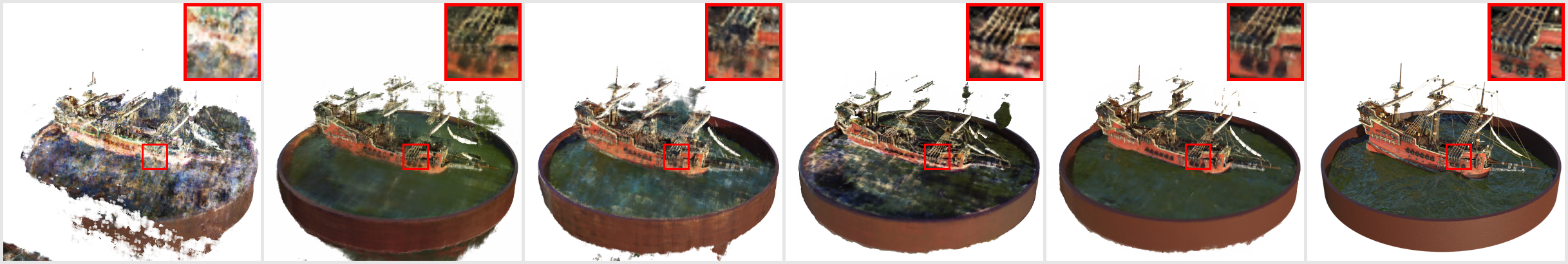
(a) Realistic Synthetic 360^∘ 4-view

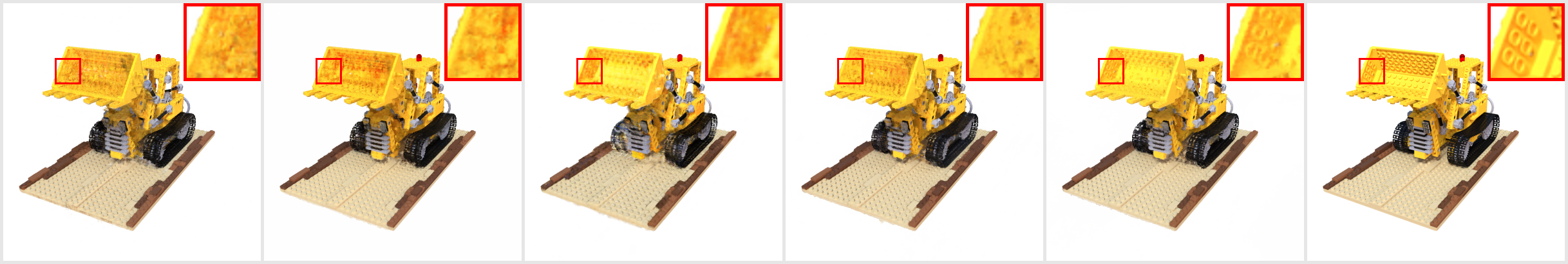
(b) Realistic Synthetic 360^∘ 8-view

mip-NeRF [1]

RegNeRF [25]

FreeNeRF‡ [45]

FlipNeRF [33]

HourglassNeRF

Ground Truth

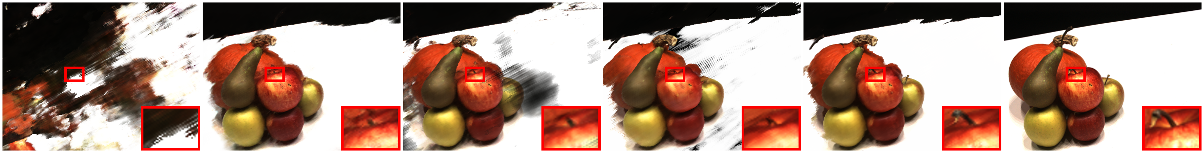
(c) DTU 3-view

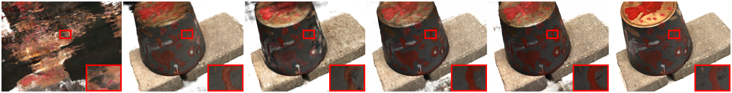
(d) DTU 6-view

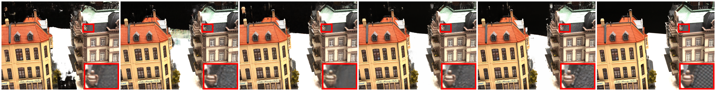
(e) DTU 9-view

Figure 7: Qualitative comparisons on Realistic Synthetic 360^∘ and DTU. Our HourglassNeRF achieves notable rendering quality with better capturing fine details. $\ddagger$ indicates the W&B prior.

DTU.

Tab. 4 shows the quantitative comparisons on DTU. Our HourglassNeRF outperforms the baseline FlipNeRF, and achieves competitive results overall. As demonstrated in Fig. 7, ours shows notable outcomes with sharply rendered textures. FreeNeRF is trained with the black and white prior assuming the estimated black and white color as the background and table, respectively, which is a highly strong assumption specific to the dataset, and achieves degenerate results without the prior. However, our HourglassNeRF utilizes the Lambertian assumption, which is a strong but effective condition for few-shot scenario, reducing the heuristic components for the training framework. Furthermore, as shown in Fig. 9, while FreeNeRF achieves high-quality rendering, it relies on a white and black prior, i.e. a highly heuristic approach given the dataset’s characteristics. In contrast, our HourglassNeRF shows competitive performance without relying on such priors.

	PSNR $\uparrow$	SSIM $\uparrow$	LPIPS $\downarrow$	Average $\downarrow$
FreeNeRF‡ [45]	19.92	0.781	0.125	0.086
FreeNeRF [45]	19.23	0.769	0.149	0.103
HourglassNeRF	19.85	0.773	0.146	0.096

FreeNeRF‡ [45]

FreeNeRF [45]

HourglassNeRF

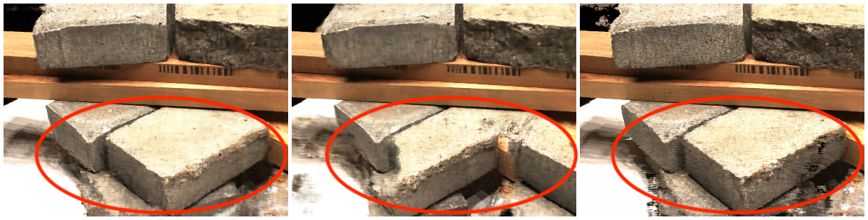
Figure 8: Additional comparison with FreeNeRF on DTU 3-view. Although FreeNeRF achieves high-quality of rendering with only a few images, it depends on the white and black prior, which is highly heuristic based on the characteristics of dataset. Our HourglassNeRF achieves comparable performance to FreeNeRF without the heuristic prior for training. $\ddagger$ denotes the W&B prior.

	PSNR $\uparrow$	SSIM $\uparrow$	LPIPS $\downarrow$	Average $\downarrow$
Ref-NeRF [40]	17.10	0.821	0.190	0.142
FreeNeRF [45]	16.99	0.828	0.157	0.131
FlipNeRF [33]	18.14	0.847	0.141	0.109
HourglassNeRF	18.68	0.851	0.141	0.107

FreeNeRF [45]

FlipNeRF [33]

Ours

GT

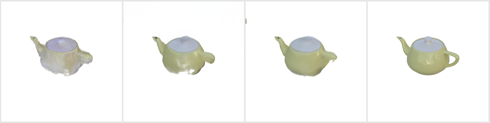
Figure 9: Quantitative and qualitative results on Shiny Blender 4-view. While FlipNeRF demonstrates competitive performance by utilizing flipped specular reflection rays, which are physically aligned with the non-Lambertian surfaces, our approach consistently outperforms FlipNeRF and other comparative methods.

Shiny Blender.

We additionally compare our HourglassNeRF and other methods on Shiny Blender, which is largely non-Lambertian, as in Fig. 9. Although FlipNeRF achieves competitive performance thanks to its ray augmentation strategy utilizing specular reflection, which accords with the non-Lambertian surfaces, ours still outperforms other methods including FlipNeRF. We conjecture that under the few-shot setting where the major challenge is to learn 3D geometry effectively while appropriately avoiding the overfitting, our high-frequency regularization effect plays an important role despite contradicting physical assumptions.

5 Conclusion

In this work, we have approached the few-shot novel view synthesis from the perspective of a novel ray parameterization. Our HourglassNeRF casts an hourglass as an augmented ray, which adaptively regularizes the high-frequency components based on the target pixel photo-consistency. Through our proposed hourglass casting strategy, our HourglassNeRF effectively prevents overfitting to high-frequency components while achieving sharp fine details. Furthermore, compared to the baseline FlipNeRF, ours is a more physically grounded training framework by conceptualizing our hourglass as a featurized bundle of flipped diffuse reflection rays with our proposed luminance consistency regularization. As the hourglass covers the wider area of unseen views than a single ray, our HourglassNeRF is trained more efficiently without casting multiple augmented rays per original ray. Our HourglassNeRF achieves the SOTA or competitive performance compared to other methods under various few-shot scenarios. We expect that our HourglassNeRF is able to inspire a meaningful approach in the few-shot NeRF framework.

Limitations and future work.

Since our HourglassNeRF is based upon the Lambertian assumption, we regard all reflection rays as diffuse even if they are from a shiny surface. As a result, although our HourglassNeRF shows superior performance to other methods on the Shiny Blender dataset mainly consisting of non-Lambertian surfaces, the characteristics of the object’s surface are not adequately considered. Using both specular and diffuse reflection rays adaptively based on the estimated texture of the surface can be a meaningful direction for future work.

HourglassNeRF: Casting an Hourglass as a Bundle of Rays for Few-shot Neural Rendering
–Supplementary Material–

Table 5: Hyperparameters and balancing weights. Since our HourglassNeRF is built upon FlipNeRF, we follow the training details for other hyperparameters, which are not mentioned here, as FlipNeRF.

Hyperparameter	Realistic Synthetic 360∘ [24]		DTU [11]			Shiny Blender [40]
& Balancing Weights	4-view	8-view	3-view	6-view	9-view	4-view
LR	$[1\mathrm{e}{-3},1\mathrm{e}{-5}]$		$[2\mathrm{e}{-3},2\mathrm{e}{-5}]$			$[1\mathrm{e}{-3},1\mathrm{e}{-5}]$
Warm-up Iter.	512	1024	512	2048		512
$\eta_{\text{Ori.}}(\text{for }\mathcal{L}_{\text{Ori.}})$	$1\mathrm{e}{-1}$	$1\mathrm{e}{-2}$	$1\mathrm{e}{-1}$	$1\mathrm{e}{-2}$		$1\mathrm{e}{-1}$
$\eta_{\text{lum.}}(\text{for }l_{\text{lum.}})$	$1\mathrm{e}{-3}$	$1\mathrm{e}{-4}$	$1\mathrm{e}{-3}$	$1\mathrm{e}{-4}$	$1\mathrm{e}{-5}$	$1\mathrm{e}{-3}$
$\tilde{\eta}_{\text{lum.}}(\text{for }\tilde{l}_{\text{lum.}})$	$1\mathrm{e}{-4}$	$1\mathrm{e}{-5}$	$1\mathrm{e}{-4}$	$1\mathrm{e}{-5}$	$1\mathrm{e}{-6}$	$1\mathrm{e}{-4}$

6 Experimental Setting

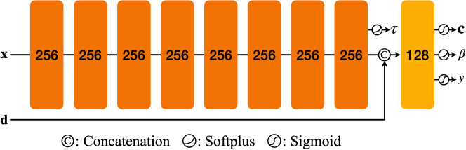
Figure 10: Network architecture of HourglassNeRF. Our HourglassNeRF estimates the additional output $y$, i.e. the relative luminance for our auxiliary luminance estimation task.

Implementational details.

Our HourglassNeRF is implemented upon FlipNeRF [33], and we follow its overall training scheme. We utilize the scene space annealing strategy during the initial training phase following [25, 34, 33]. Furthermore, we adopt the initial warm up and exponential decay for the learning rate. We use the Adam optimizer [15] with gradient clipping set to 0.1 for both each element of the gradient value and the gradient’s norm. Our HourglassNeRF is trained for 500 pixel epochs using a batch size of 4,096 on four NVIDIA RTX 3090 GPUs. Additionally, since our proposed hourglass encompasses broader areas of unseen views compared to a single ray, we set the masking threshold $\psi$ as 45^∘, which is smaller than that of FlipNeRF, to avoid over-regularization effect of augmented rays. The related experiment is demonstrated in Tab. 7.

Hyperparameters.

For additional details on hyperparameters and loss balancing terms based on training views and datasets, kindly refer to Tab. 5. Note that our HourglassNeRF follows the same hyperparameters as FlipNeRF for other training losses and schemes which are not specified in Tab. 5.

7 Further Details of Method

Architectural details.

Our HourglassNeRF leverages the network architecture of mip-NeRF [1], which is commonly used in several few-shot NeRF models [45, 25, 33, 34]. Moreover, our HourglassNeRF additionally estimates the relative luminance $y$. Kindly refer to more details in Fig. 10.

Total loss.

Our HourglassNeRF is trained to maximize the log-likelihood of the target pixel $\mathbf{c}_{\text{GT}}$ for both sets of original input rays $\mathcal{R}$ and our proposed hourglasses $\tilde{\mathcal{R}}$, as well as to minimize the mean squared errors (MSE) between the ground-truth and estimated pixel values. Except our proposed $\mathcal{L}_{\text{lum.}}$, we use the same training losses as those of FlipNeRF. Note that we use $\mathcal{L}_{\text{MSE}}$ only for $\mathcal{R}$ and exploit a batch of hourglasses instead of flipped reflection rays, which are used in FlipNeRF. Summing up, the total loss over a batch is calculated as follows:

$$\begin{split}\mathcal{L}_{\text{Total}}&=\mathcal{L}_{\text{MSE}}+\mathcal{L}_{\text{lum.}}+\eta_{\text{NLL}}\mathcal{L}_{\text{NLL}}+\tilde{\eta}_{\text{NLL}}\tilde{\mathcal{L}}_{\text{NLL}}\\ &+\eta_{\text{UE}}\mathcal{L}_{\text{UE}}+\tilde{\eta}_{\text{UE}}\tilde{\mathcal{L}}_{\text{UE}}^{\prime}+\eta_{\text{BFC}}\mathcal{L}_{\text{BFC}}+\eta_{\text{Ori.}}\mathcal{L}_{\text{Ori.}},\\ &\text{where}\quad\mathcal{L}_{\text{lum.}}=\eta_{\text{lum.}}l_{\text{lum.}}+\tilde{\eta}_{\text{lum.}}\tilde{l}_{\text{lum.}}.\end{split}$$ (12)

$\eta$’s and $\tilde{\eta}$’s represent the loss balancing weights for the original input rays and additional hourglasses, respectively.

Table 6: Effect of Viewing direction jittering. On Realistic Synthetic 360^∘ 4-view, we are able to achieve marginal performance improvement while still outperforming FlipNeRF without the jittering strategy.

	PSNR $\uparrow$	SSIM $\uparrow$	LPIPS $\downarrow$	Average Err. $\downarrow$
FlipNeRF [33]	16.47	0.866	0.091	0.095
HourglassNeRF
w/o view. jitter.	16.66	0.869	0.087	0.093
w/ view. jitter.	16.86	0.873	0.084	0.091

Table 7: Comparison of masking thresholds. Our HourglassNeRF excludes a set of hourglasses, whose angle $\theta$ between the original input ray is over $\psi$, i.e. the target pixel photo-consistency is relatively low considering the threshold $\psi$, from a training batch. $\psi=180^{\circ}\text{(None)}$ uses a whole batch of newly generated hourglasses.

$\psi$	PSNR $\uparrow$	SSIM $\uparrow$	LPIPS $\downarrow$	Average Err. $\downarrow$
180∘ (None)	18.15	0.749	0.179	0.120
90∘	18.63	0.762	0.163	0.110
75∘	19.02	0.764	0.156	0.105
60∘	18.94	0.766	0.154	0.105
45∘	19.85	0.773	0.146	0.096
30∘	18.78	0.765	0.160	0.107
15∘	18.65	0.761	0.163	0.111

8 Additional Experiments

Viewing direction jittering.

For Realistic Synthetic 360^∘ [24] and Shiny Blender [40], which consist of inward-facing synthetic scenes with objects located at the center, we adopt the viewing direction jittering, which is a minor additional strategy slightly improving the performance. We simply add the Gaussian random noise to the input viewing direction $\mathbf{d}$ to improve the robustness for the slight change of viewpoints. As shown in Tab. 7, we are able to achieve marginal improvement of rendering quality while still outperforming its baseline, FlipNeRF, even without the jittering.

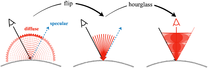
Figure 11: Hourglass as a bundle of flipped diffuse reflection rays. Assuming a Lambertian surface, which primarily results in diffuse reflection, we treat our proposed hourglass as equivalent to a featurized bundle of flipped diffuse reflection rays. Leveraging the Lambertian surface’s property of luminance consistency, we propose an effective regularization technique that trains the relative luminance outputs of the original ray and additional hourglass to match the GT relative luminance. Technically, like in Fig. 2, although the ray is spanned over the surface as in the original NeRF, we simplify the illustration for brevity.

Masking thresholds.

Our HourglassNeRF utilizes an additional batch of hourglasses covering a broader area of unseen views, which are conceptualized as a bundle of flipped diffuse reflection rays as shown in Fig. 11, and the high-frequency components of samples along an hourglass are adaptively regularized depending on the angle between the original input direction and the estimated normal vector, i.e. the target pixel photo-consistency. As a result, with the same $\psi=90^{\circ}$ as FlipNeRF, our HourglassNeRF might suffer from the performance degradation due to over-regularization. As demonstrated in Tab. 7, our HourglassNeRF achieves the best result with $\psi=45^{\circ}$. The larger $\psi$ becomes than $45^{\circ}$, the worse the performance, as an hourglass covering too wide area of unseen views leads to over-regularization, which adversely affects the training. On the other hand, a smaller $\psi$ than $45^{\circ}$ also leads to poorer performance, as the newly generated hourglasses are excessively filtered, resulting in only a limited number of augmented hourglasses being utilized for training. Note that the masking threshold $\psi$ depends on the characteristics of casting ray rather than the hyperparameter which needs to be finetuned elaboratively.

Table 8: Additional quantitative comparison on DTU. $\dagger$ and $\ddagger$ indicate fine-tuning and W&B prior, respectively.

	Method	PSNR $\uparrow$			SSIM $\uparrow$			LPIPS $\downarrow$			Avg. Err. $\downarrow$
		3-view	6-view	9-view	3-view	6-view	9-view	3-view	6-view	9-view	3-view	6-view	9-view
Mip-NeRF [1]	-	8.68	16.54	23.58	0.571	0.741	0.879	0.353	0.198	0.092	0.323	0.148	0.056
PixelNeRF [46]	Pre-training	16.82	19.11	20.40	0.695	0.745	0.768	0.270	0.232	0.220	0.147	0.115	0.100
PixelNeRF† [46]		18.95	20.56	21.83	0.710	0.753	0.781	0.269	0.223	0.203	0.125	0.104	0.090
SRF [5]		15.32	17.54	18.35	0.671	0.730	0.752	0.304	0.250	0.232	0.171	0.132	0.120
SRF† [5]		15.68	18.87	20.75	0.698	0.757	0.785	0.281	0.225	0.205	0.162	0.114	0.093
MVSNeRF [4]		18.63	20.70	22.40	0.769	0.823	0.853	0.197	0.156	0.135	0.113	0.088	0.068
MVSNeRF† [4]		18.54	20.49	22.22	0.769	0.822	0.853	0.197	0.155	0.135	0.113	0.089	0.069
DietNeRF [9]	Regularization	11.85	20.63	23.83	0.633	0.778	0.823	0.314	0.201	0.173	0.243	0.101	0.068
RegNeRF [25]		18.89	22.20	24.93	0.745	0.841	0.884	0.190	0.117	0.089	0.112	0.071	0.047
MixNeRF [34]		18.95	22.30	25.03	0.744	0.835	0.879	0.203	0.102	0.065	0.113	0.066	0.042
FreeNeRF‡ [45]		19.92	23.25	25.38	0.781	0.838	0.877	0.125	0.085	0.057	0.086	0.058	0.038
FlipNeRF [33]		19.55	22.45	25.12	0.767	0.839	0.882	0.180	0.098	0.062	0.101	0.064	0.041
HourglassNeRF		19.85	22.73	25.14	0.773	0.842	0.886	0.146	0.084	0.057	0.096	0.060	0.040

Additional results.

The quantitative comparisons including the pre-training methods on DTU are demonstrated in Tab. 8. Our HourglassNeRF achieves competitive performance among the SOTA methods.

References

- [1] Barron, J.T., Mildenhall, B., Tancik, M., Hedman, P., Martin-Brualla, R., Srinivasan, P.P.: Mip-nerf: A multiscale representation for anti-aliasing neural radiance fields. In: Proceedings of the IEEE/CVF International Conference on Computer Vision. pp. 5855–5864 (2021)
- [2] Barron, J.T., Mildenhall, B., Verbin, D., Srinivasan, P.P., Hedman, P.: Mip-nerf 360: Unbounded anti-aliased neural radiance fields. In: Proceedings of the IEEE/CVF Conference on Computer Vision and Pattern Recognition. pp. 5470–5479 (2022)
- [3] Chang, Y., Kim, Y., Seo, S., Yi, J., Kwak, N.: Fast sun-aligned outdoor scene relighting based on tensorf. In: Proceedings of the IEEE/CVF Winter Conference on Applications of Computer Vision. pp. 3626–3636 (2024)
- [4] Chen, A., Xu, Z., Zhao, F., Zhang, X., Xiang, F., Yu, J., Su, H.: Mvsnerf: Fast generalizable radiance field reconstruction from multi-view stereo. In: Proceedings of the IEEE/CVF International Conference on Computer Vision. pp. 14124–14133 (2021)
- [5] Chibane, J., Bansal, A., Lazova, V., Pons-Moll, G.: Stereo radiance fields (srf): Learning view synthesis for sparse views of novel scenes. In: Proceedings of the IEEE/CVF Conference on Computer Vision and Pattern Recognition. pp. 7911–7920 (2021)
- [6] Deng, K., Liu, A., Zhu, J.Y., Ramanan, D.: Depth-supervised nerf: Fewer views and faster training for free. In: Proceedings of the IEEE/CVF Conference on Computer Vision and Pattern Recognition. pp. 12882–12891 (2022)
- [7] Gao, C., Saraf, A., Kopf, J., Huang, J.B.: Dynamic view synthesis from dynamic monocular video. In: Proceedings of the IEEE/CVF International Conference on Computer Vision. pp. 5712–5721 (2021)
- [8] Isaac-Medina, B.K., Willcocks, C.G., Breckon, T.P.: Exact-nerf: An exploration of a precise volumetric parameterization for neural radiance fields. In: Proceedings of the IEEE/CVF Conference on Computer Vision and Pattern Recognition. pp. 66–75 (2023)
- [9] Jain, A., Tancik, M., Abbeel, P.: Putting nerf on a diet: Semantically consistent few-shot view synthesis. In: Proceedings of the IEEE/CVF International Conference on Computer Vision. pp. 5885–5894 (2021)
- [10] Jang, W., Agapito, L.: Codenerf: Disentangled neural radiance fields for object categories. In: Proceedings of the IEEE/CVF International Conference on Computer Vision. pp. 12949–12958 (2021)
- [11] Jensen, R., Dahl, A., Vogiatzis, G., Tola, E., Aanæs, H.: Large scale multi-view stereopsis evaluation. In: Proceedings of the IEEE conference on computer vision and pattern recognition. pp. 406–413 (2014)
- [12] Jiang, W., Yi, K.M., Samei, G., Tuzel, O., Ranjan, A.: Neuman: Neural human radiance field from a single video. In: European Conference on Computer Vision. pp. 402–418. Springer (2022)
- [13] Johari, M.M., Lepoittevin, Y., Fleuret, F.: Geonerf: Generalizing nerf with geometry priors. In: Proceedings of the IEEE/CVF Conference on Computer Vision and Pattern Recognition. pp. 18365–18375 (2022)
- [14] Kim, M., Seo, S., Han, B.: Infonerf: Ray entropy minimization for few-shot neural volume rendering. In: Proceedings of the IEEE/CVF Conference on Computer Vision and Pattern Recognition. pp. 12912–12921 (2022)
- [15] Kingma, D.P., Ba, J.: Adam: A method for stochastic optimization. arXiv preprint arXiv:1412.6980 (2014)
- [16] Kwak, M., Song, J., Kim, S.: Geconerf: Few-shot neural radiance fields via geometric consistency. arXiv preprint arXiv:2301.10941 (2023)
- [17] Li, J., Feng, Z., She, Q., Ding, H., Wang, C., Lee, G.H.: Mine: Towards continuous depth mpi with nerf for novel view synthesis. In: Proceedings of the IEEE/CVF International Conference on Computer Vision. pp. 12578–12588 (2021)
- [18] Li, T., Slavcheva, M., Zollhoefer, M., Green, S., Lassner, C., Kim, C., Schmidt, T., Lovegrove, S., Goesele, M., Newcombe, R., et al.: Neural 3d video synthesis from multi-view video. In: Proceedings of the IEEE/CVF Conference on Computer Vision and Pattern Recognition. pp. 5521–5531 (2022)
- [19] Li, Z., Wang, Q., Cole, F., Tucker, R., Snavely, N.: Dynibar: Neural dynamic image-based rendering. In: Proceedings of the IEEE/CVF Conference on Computer Vision and Pattern Recognition. pp. 4273–4284 (2023)
- [20] Lin, C.H., Gao, J., Tang, L., Takikawa, T., Zeng, X., Huang, X., Kreis, K., Fidler, S., Liu, M.Y., Lin, T.Y.: Magic3d: High-resolution text-to-3d content creation. In: Proceedings of the IEEE/CVF Conference on Computer Vision and Pattern Recognition. pp. 300–309 (2023)
- [21] Liu, R., Wu, R., Van Hoorick, B., Tokmakov, P., Zakharov, S., Vondrick, C.: Zero-1-to-3: Zero-shot one image to 3d object. In: Proceedings of the IEEE/CVF International Conference on Computer Vision. pp. 9298–9309 (2023)
- [22] Liu, Y., Peng, S., Liu, L., Wang, Q., Wang, P., Theobalt, C., Zhou, X., Wang, W.: Neural rays for occlusion-aware image-based rendering. In: Proceedings of the IEEE/CVF Conference on Computer Vision and Pattern Recognition. pp. 7824–7833 (2022)
- [23] Metzer, G., Richardson, E., Patashnik, O., Giryes, R., Cohen-Or, D.: Latent-nerf for shape-guided generation of 3d shapes and textures. In: Proceedings of the IEEE/CVF Conference on Computer Vision and Pattern Recognition. pp. 12663–12673 (2023)
- [24] Mildenhall, B., Srinivasan, P.P., Tancik, M., Barron, J.T., Ramamoorthi, R., Ng, R.: Nerf: Representing scenes as neural radiance fields for view synthesis. Communications of the ACM 65(1), 99–106 (2021)
- [25] Niemeyer, M., Barron, J.T., Mildenhall, B., Sajjadi, M.S., Geiger, A., Radwan, N.: Regnerf: Regularizing neural radiance fields for view synthesis from sparse inputs. In: Proceedings of the IEEE/CVF Conference on Computer Vision and Pattern Recognition. pp. 5480–5490 (2022)
- [26] Poole, B., Jain, A., Barron, J.T., Mildenhall, B.: Dreamfusion: Text-to-3d using 2d diffusion. In: The Eleventh International Conference on Learning Representations (2022)
- [27] Poynton, C.: Digital video and HD: Algorithms and Interfaces. Elsevier (2012)
- [28] Poynton, C.A.: A technical introduction to digital video. John Wiley & Sons, Inc. (1996)
- [29] Pumarola, A., Corona, E., Pons-Moll, G., Moreno-Noguer, F.: D-nerf: Neural radiance fields for dynamic scenes. In: Proceedings of the IEEE/CVF Conference on Computer Vision and Pattern Recognition. pp. 10318–10327 (2021)
- [30] Reinhard, E., Stark, M., Shirley, P., Ferwerda, J.: Photographic tone reproduction for digital images. In: Seminal Graphics Papers: Pushing the Boundaries, Volume 2, pp. 661–670 (2023)
- [31] Rematas, K., Martin-Brualla, R., Ferrari, V.: Sharf: Shape-conditioned radiance fields from a single view. In: International Conference on Machine Learning. pp. 8948–8958. PMLR (2021)
- [32] Roessle, B., Barron, J.T., Mildenhall, B., Srinivasan, P.P., Nießner, M.: Dense depth priors for neural radiance fields from sparse input views. In: Proceedings of the IEEE/CVF Conference on Computer Vision and Pattern Recognition. pp. 12892–12901 (2022)
- [33] Seo, S., Chang, Y., Kwak, N.: Flipnerf: Flipped reflection rays for few-shot novel view synthesis. In: Proceedings of the IEEE/CVF International Conference on Computer Vision. pp. 22883–22893 (2023)
- [34] Seo, S., Han, D., Chang, Y., Kwak, N.: Mixnerf: Modeling a ray with mixture density for novel view synthesis from sparse inputs. In: Proceedings of the IEEE/CVF Conference on Computer Vision and Pattern Recognition. pp. 20659–20668 (2023)
- [35] Song, L., Li, Z., Gong, X., Chen, L., Chen, Z., Xu, Y., Yuan, J.: Harnessing low-frequency neural fields for few-shot view synthesis. arXiv preprint arXiv:2303.08370 (2023)
- [36] Su, S.Y., Yu, F., Zollhöfer, M., Rhodin, H.: A-nerf: Articulated neural radiance fields for learning human shape, appearance, and pose. Advances in Neural Information Processing Systems 34, 12278–12291 (2021)
- [37] Tretschk, E., Tewari, A., Golyanik, V., Zollhöfer, M., Lassner, C., Theobalt, C.: Non-rigid neural radiance fields: Reconstruction and novel view synthesis of a dynamic scene from monocular video. In: Proceedings of the IEEE/CVF International Conference on Computer Vision. pp. 12959–12970 (2021)
- [38] Trevithick, A., Yang, B.: Grf: Learning a general radiance field for 3d representation and rendering. In: Proceedings of the IEEE/CVF International Conference on Computer Vision. pp. 15182–15192 (2021)
- [39] Truong, P., Rakotosaona, M.J., Manhardt, F., Tombari, F.: Sparf: Neural radiance fields from sparse and noisy poses. In: Proceedings of the IEEE/CVF Conference on Computer Vision and Pattern Recognition. pp. 4190–4200 (2023)
- [40] Verbin, D., Hedman, P., Mildenhall, B., Zickler, T., Barron, J.T., Srinivasan, P.P.: Ref-nerf: Structured view-dependent appearance for neural radiance fields. In: 2022 IEEE/CVF Conference on Computer Vision and Pattern Recognition (CVPR). pp. 5481–5490. IEEE (2022)
- [41] Wang, Q., Wang, Z., Genova, K., Srinivasan, P.P., Zhou, H., Barron, J.T., Martin-Brualla, R., Snavely, N., Funkhouser, T.: Ibrnet: Learning multi-view image-based rendering. In: Proceedings of the IEEE/CVF Conference on Computer Vision and Pattern Recognition. pp. 4690–4699 (2021)
- [42] Wang, Z., Bovik, A.C., Sheikh, H.R., Simoncelli, E.P.: Image quality assessment: from error visibility to structural similarity. IEEE transactions on image processing 13(4), 600–612 (2004)
- [43] Weng, C.Y., Curless, B., Srinivasan, P.P., Barron, J.T., Kemelmacher-Shlizerman, I.: Humannerf: Free-viewpoint rendering of moving people from monocular video. In: Proceedings of the IEEE/CVF conference on computer vision and pattern Recognition. pp. 16210–16220 (2022)
- [44] Xu, H., Alldieck, T., Sminchisescu, C.: H-nerf: Neural radiance fields for rendering and temporal reconstruction of humans in motion. Advances in Neural Information Processing Systems 34, 14955–14966 (2021)
- [45] Yang, J., Pavone, M., Wang, Y.: Freenerf: Improving few-shot neural rendering with free frequency regularization. In: Proceedings of the IEEE/CVF Conference on Computer Vision and Pattern Recognition. pp. 8254–8263 (2023)
- [46] Yu, A., Ye, V., Tancik, M., Kanazawa, A.: pixelnerf: Neural radiance fields from one or few images. In: Proceedings of the IEEE/CVF Conference on Computer Vision and Pattern Recognition. pp. 4578–4587 (2021)
- [47] Zhang, R., Isola, P., Efros, A.A., Shechtman, E., Wang, O.: The unreasonable effectiveness of deep features as a perceptual metric. In: Proceedings of the IEEE conference on computer vision and pattern recognition. pp. 586–595 (2018)
- [48] Zhao, F., Yang, W., Zhang, J., Lin, P., Zhang, Y., Yu, J., Xu, L.: Humannerf: Efficiently generated human radiance field from sparse inputs. In: Proceedings of the IEEE/CVF Conference on Computer Vision and Pattern Recognition. pp. 7743–7753 (2022)