Abstract: We estimate the short-run effects of severe weather shocks on local economic activity and assess cross-border spillovers operating through economic linkages between U.S. states. We measure weather shocks using a detailed county-level database on emergency declarations triggered by natural disasters and estimate their impacts with a monthly Global Vector Autoregressive (GVAR) model for the U.S. states. Impulse responses highlight significant country-wide macroeconomic effects of weather shocks hitting individual regions. We also show that (i) taking into account economic interconnections between states allows capturing much stronger spillover effects than those associated with mere spatial adjacency, (ii) geographical heterogeneity is critical for assessing country-wide effects of weather shocks, and (iii) network effects amplify the local impacts of these shocks.
Keywords: Global VAR, natural disasters, spillovers, weather shocks, United States, climate change
JEL Codes: C32, R11, Q51, Q54. ^(∗) Corresponding author: Graziano Moramarco, Department of Economics, University of Bologna, Piazza Scaravilli 2, Bologna, Italy. Email: graziano.moramarco@unibo.it. Acknowledgments: For this research, Graziano Moramarco gratefully acknowledges funding from the European Union and Ministero dell’Università e della Ricerca - PON Ricerca e Innovazione 2014-2020.

1 Introduction

Climate-related risks are now regarded as major sources of economic vulnerability. These risks are associated with adverse climatic events (physical risks) or induced by the process of adjustment towards a low-carbon economy (transition risks). Extreme weather events are the primary types of physical risks and are becoming more frequent as a result of climate change (IPCC, 2023). Evaluating their potentially long-lasting economic impacts (Batten, , 2018; Hsiang and Jina, , 2014) requires considering not only local effects but also spillovers across interconnected economic systems (Benzie, , 2021; Cashin et al., , 2017).

In this study we examine the impact of severe weather shocks on state-level economic activity in the United States, considering the cross-border spillovers resulting from economic interconnections among states and regions. We rely on a monthly Global Vector Autoregressive (GVAR) model (Pesaran et al., , 2004) that captures economic interrelationships between states and regions using bilateral trade flows within the U.S. and include a proxy of severe weather shocks, based on a detailed database of emergency declarations triggered by natural disasters.

We find that weather shocks generate direct negative macroeconomic effects at the local level and significant negative spillovers to U.S. regions not directly affected. Furthermore, we perform several robustness checks to evaluate the quantitative and qualitative relevance of our results. We start assessing the importance of economic interconnections when measuring spillovers, rather than simply considering spatial proximity of states. Therefore, we compare our baseline GVAR model with an alternative GVAR specification where states are connected by a spatial adjacency matrix. Moreover, our model allows for parameter heterogeneity between states. We thus evaluate the importance of this feature by comparing our GVAR model with its “homogeneous-parameter counterpart”, namely a spatial panel dynamic model. Next, we consider a country-wide regression for the U.S. to check whether disaggregation at the state level matters at all. We show that disaggregation, parameter heterogeneity and economic linkages between states are key for quantifying spillover effects and the overall impact of weather shocks in the U.S. Lastly, we provide a measure of the impact of spillovers for each state, by comparing responses to weather shocks between the GVAR model – that allows for spillovers – and individual state-specific Autoregressive Distributed Lag (ARDL) models where spillovers are implicitly muted.

The paper is related to several streams of literature. First, it adds to the rapidly growing literature on the macroeconomic effects of extreme weather events and climate change (see e.g. Boldin and Wright, , 2015; Burke et al., , 2015; Colacito et al., , 2019; Dell et al., , 2014; Colombo and Ferrara, , 2024; Billio et al., , 2020; Ahmadi et al., , 2022). In particular, it contributes to the strand of research on cross-border impacts of climate change (Benzie, , 2021; Carter et al., , 2021; Feng et al., , 2023). There is ample evidence that the effects of natural disasters propagate through international trade and production networks (Barrot and Sauvagnat, , 2016; Boehm et al., , 2019; Carvalho et al., , 2020; Feng et al., , 2023; Forslid and Sanctuary, , 2023; Kashiwagi et al., , 2021). Our paper is also related to the literature on climate econometrics (see e.g. Burke et al., , 2015; Hsiang, , 2016; Kahn et al., , 2021). Focusing on the methodology, it is worth pointing out that the GVAR framework has been used to investigate the international spillovers of El Niño weather shocks by Cashin et al., (2017).

Four papers, to the best of our knowledge, are closely related to our work, in that they have focused on the effects of climate and weather extremes on the U.S. economy. Mohaddes et al., (2022) and Natoli, (2023) investigate the long-term macroeconomic effects of climate change across the U.S. over the period 1963–2016. Unlike our analysis, these authors focus on temperature and precipitation anomalies rather than natural disasters and do not assess spillover effects between states. Kim et al., (2021) investigate the effects of severe weather conditions, proxied by the Actuaries Climate Index, on the aggregate U.S. economy over the period 1963-2019. They find that the effects have become significant only in recent years. Tran and Wilson, (2020) study the long-run impact of natural disasters on income using our same proxy based on disaster declarations. Our paper relies on monthly data and focuses on short-run impacts, thus we complement their analysis based on annual data and concentrating on long-run impacts.

The rest of the paper is organized as follows. Section 2 presents the data, with a particular focus on our proxy for severe weather shocks, Section 3 discusses the econometric model, Section 4 presents the results, and Section 5 concludes. A Supplement with further results completes the paper.

2 Data

2.1 Weather shocks

We build a novel monthly proxy of weather shocks using the Disaster Declarations Summary dataset maintained by the U.S. Federal Emergency Management Agency (FEMA). FEMA, established in 1979 with an executive order signed by President Carter, is part of the Department of Homeland Security and is responsible for coordinating the federal government’s relief efforts after natural or man-made domestic disasters. All federally declared disasters since 1953 are collected in the Disaster Declarations Summary. For each declaration, the database provides detailed information on the states and counties affected by the disaster, its beginning and end dates, as well as on the type of disaster.

Because the Congress has broadened FEMA’s mandate over the years, the number of declarations has also grown since its inception and in particular after 1988. In fact, the Stafford Disaster Relief and Emergency Assistance Act of 1988 established that a presidential declaration triggers financial and physical assistance through FEMA. To avoid issues related to this policy shift induced by the Stafford Act, we restrict the sample to events from January 1990 through December 2019. We consider three types of disaster declarations that differ in terms of the events triggering them, their scope, as well as the amount of funds and type of assistance provided. These are: Emergency Declarations, Major Disaster Declarations, and Fire Management Assistance Declarations.

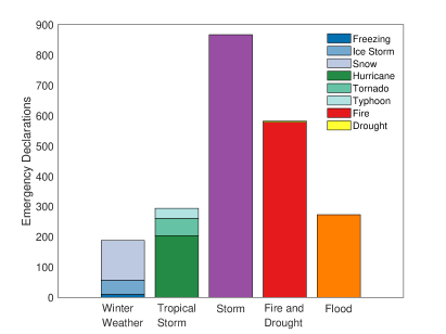
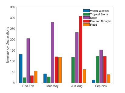
Figure 1: Emergency declarations by type and season: January 1990 to December 2019

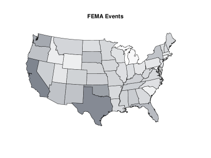
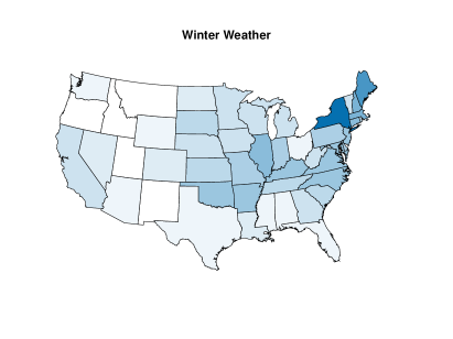
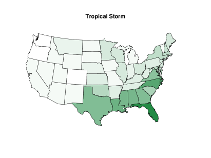
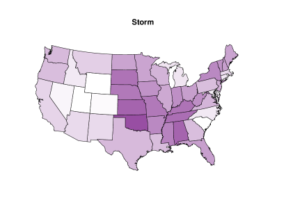
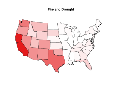
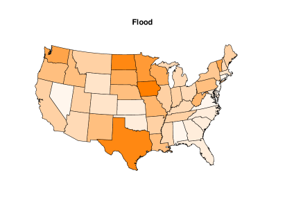
Figure 2: Emergency declarations by state and type of event: 1990-2019

Notes: the maps show the count of emergency declarations (total and by type of event). Colors range from lighter to darker as the count of events grows. Hawaii and Alaska are omitted for better display.

We focus on declarations caused by events that are directly related to weather conditions. In particular, we consider the following main events that group the weather-related declarations in FEMA’s database: winter weather (i.e. freezing, ice storms, snow), tropical storms (i.e. hurricanes, typhoons and tornadoes), storms (i.e. coastal and severe storms), fire, flood, drought. Figure 1 displays the events examined in our analysis. The left panel shows that storms and fires are associated with the majority of declarations. In the right panel of the figure, we report the distribution of events over different seasons that highlights that most events exhibit the expected seasonal patterns. Figure 2 shows the count of declarations by state and by type. Darker colors indicate a higher number of events. If we do not distinguish by event type – upper left panel – we can see that emergency declarations are evenly distributed across states. The same holds true for storms and floods. On the contrary, declarations triggered by severe winter weather, tropical storms, fires, and drought are geographically concentrated in the northeast, southeast, and west of the U.S., respectively. Alternative representations of the maps in Figure 2, based either on the count of declarations weighted by the state population density or aggregated over U.S. climate regions, are presented in the online Appendix.

Measuring weather shocks with disaster declarations. We construct our proxy of weather shocks as follows. First, for each state $i$ we create a dummy variable that takes value one if a weather-related disaster was declared in month $t$, and zero otherwise ($emergency_{it}$). Second, we multiply this dummy variable by a weight, given by the ratio between the number of counties affected by the disaster ($hit_{it}$) and the number of counties (or county equivalents) in state $i$ ($counties_{i}$):

$$s_{it}=emergency_{it}\times\frac{hit_{it}}{counties_{i}}$$ (1)

Therefore, our state-level weather shock has unit value only if in a given month emergency declarations are issued for all the counties in a state. To calculate an aggregate weather shock for the U.S., we consider the number of counties hit as a share of the total number of counties in the 50 states considered in the analysis ($N_{c}=3142$):

$$s_{t}=\frac{1}{N_{c}}\sum_{i=1}^{50}emergency_{it}\times hit_{it}$$ (2)

The weather shock series for the U.S. appears in Figure 3 where we highlight the five largest shocks over the period 1990-2019. Hurricane Katrina is by far the largest event, as measured by the share of counties where emergency declarations have been issued. Figure 3 also shows that the number of declarations for the U.S. is highly volatile, but there is no visible trend, nor structural breaks in the series.

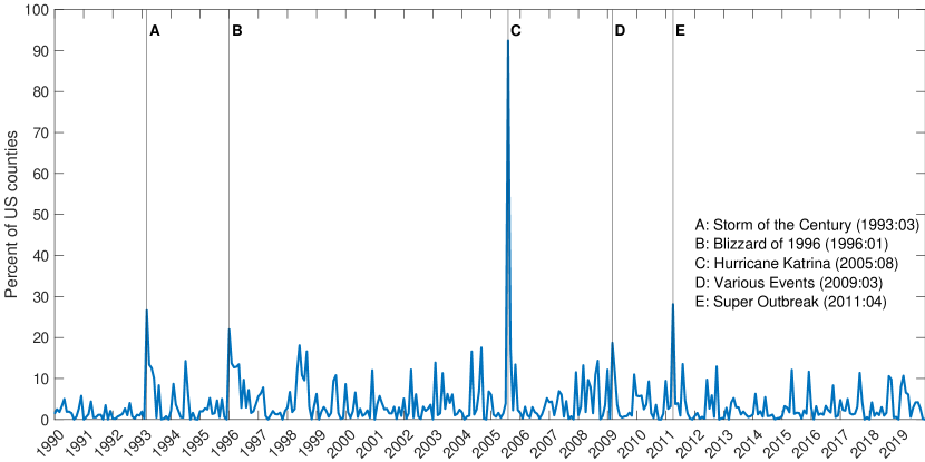
Figure 3: Weather shocks for the US

Notes: for Hurricane Katrina, emergency declarations were issued in almost all states. In states not directly hit by the hurricane the declarations go under the header “Hurricane Katrina Evacuation”.

We have considered different weighting schemes that aim to allocate more weight to areas with higher economic activity. These alternative weights are based either on resident population by state from the 2010 U.S. Census or on state-level employment rates from the Bureau of Labor Statistics. See also Boldin and Wright, (2015); Colacito et al., (2019). Results based on these proxies are qualitatively similar to those obtained relying on the share of counties hit by a natural disaster. This does not come as a surprise, given that the GVAR captures economic linkages between states and hence implicitly assigns more weight to events in hitting states that are central to the U.S. economy.

Comparison with other proxies of weather shocks. Other variables can be used to capture the effects of severe weather conditions on macroeconomic aggregates. The first option is represented by the use of weather data, which is common in the literature (see e.g. Bloesch and Gourio, , 2015; Boldin and Wright, , 2015; Colacito et al., , 2019; Wilson, , 2016; van der List and Wilson, , 2016). It is well known that measuring the weather conditions raises several problems, such as the heterogeneous quality, availability and representativeness of data from different weather stations (Dell et al., , 2014). Even after measurement issues have been taken care of, it is not clear which variables best capture weather shocks. Severe winter weather is a case in point: snowfall, temperatures, wind speed and heating degree days are just an incomplete list of alternatives available to researchers. Moreover, the societal impacts of weather events depend on the degree of preparedness of the area hit by the event. Therefore relying on weather variables is likely to introduce some measurement error and omitted variable bias in the empirical analysis, and does not guarantee to correctly identify weather events with sizable impacts on the U.S. economy.

An alternative that goes some way towards improving the identification of such events is to rely on databases explicitly designed to capture the societal impacts of weather, such as the Billion–Dollar Weather and Climate Disasters dataset. This dataset, maintained by the National Oceanic and Atmospheric Administration (NOAA, 2018), is tightly linked to our proxy. As its name suggests, the Billion–Dollar Weather and Climate Disasters dataset arbitrarily focuses only on disasters with an overall cost exceeding the threshold of one billion dollar and hence leads to a series with very low variability that might miss smaller, yet economically important events.

Yet another option, used by Boldin and Wright, (2015), is to focus on data about weather-affected jobs (i.e. the time series of absences from work due to bad weather), collected by the Bureau of Labor Statistics in the Current Population Survey. This series has three shortcomings: it does not allow us to isolate work absences due to severe winter weather from absences due to hurricanes or other events. Moreover, it only captures temporary effects of weather events and might miss economically relevant episodes that do not cause work absences but impact the supply chain. Last but not least, this measure is not suited for measuring spillovers across states: in fact absences from work in one region do not affect presence at work in other regions.

Figure 4 compares our proxy with the number of weather-affected jobs and the count of Billion Dollar Disasters. We carried out a sample cross-correlation analysis to study the lead-lag relationship between different proxies: the contemporaneous sample correlation between our proxy, the count of weather-affected jobs, and the number of Billion Dollar Disasters is equal to 0.14 and 0.01 (this becomes 0.11 if we consider the log-count), respectively. In both cases, there is no clear indication of a lead-lag relationship between the two series.

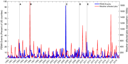
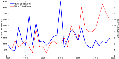
Figure 4: Alternative proxies of weather shocks for the US

To sum up, the FEMA dataset includes all disasters “of such severity and magnitude that effective response is beyond the capabilities of the state $(\ldots)$ and that supplemental federal assistance is necessary.” Extreme weather events measured in this way represent “proper” shocks in the parlance of Ramey, (2016): (i) they are exogenous with respect to the current and lagged endogenous variables of the model; (ii) they are uncorrelated with other exogenous shocks (e.g. technological, monetary or fiscal policy shocks), and (iii) they are generally unanticipated.

2.2 State-level economic variables

State-level economic activity. Our aim is to capture the impact of weather-related disasters on broad measures of economic activity that allow assessing the presence of spillover effects. Unfortunately, data on Gross State Product is only available at a quarterly frequency. The proxy of economic activity developed by Baumeister et al., (2022), referred to as weekly Economic Conditions Indicators (ECI), is suitable for our purposes. This is a composite indicator based on mixed-frequency dynamic factor models covering multiple dimensions of state-level economic activity (e.g., mobility, labor market, real activity, expectations measures, financial and households indices). Since the ECI is scaled to match four-quarter growth rates of U.S. real GDP, and we are interested in measuring the economic effects of weather shocks at a monthly frequency, we take the monthly average of the weekly index and label it Monthly Economic Conditions Indicator (MECI) hereafter. Unlike other indicators of economic activity available at the state level on a monthly basis - such as employment or hours worked - the MECI includes a broad set of both standard and non-standard variables (e.g., electricity consumption, oil rig counts, vehicle miles traveled) that allow for a more comprehensive measure, enabling a better study of any spillover effects. See Bokun et al., (2023) for an overview of state-specific variables for the U.S.

Note that we are interested in studying the effects of extreme weather, therefore it is important to assess the presence of seasonality in the MECI. The individual components of the ECI are seasonally adjusted when appropriate (refer to Baumeister et al., , 2022, for details on seasonal adjustment). Nevertheless, we further check that there are no seasonal effects left in the monthly version of the index by estimating state-specific autoregressive models augmented with month-of-the-year dummy variables. The $F$-tests indicate for all states, but North Carolina, month-of-the-year dummies are jointly non-significant, and therefore seasonal factors are not expected to affect our results.

Interstate trade flows. In GVAR models, economic interrelationships between geographical entities are most commonly measured using trade flows. To proxy bilateral trade flows between U.S. states, we use data from the latest release of the Commodity Flow Survey (CFS) in 2017. The CFS is jointly elaborated by the Bureau of Transportation Statistics (U.S. Department of Transportation) and the U.S. Census Bureau (U.S. Department of Commerce) every five years as part of the Economic Census. This survey is the primary source of data on domestic freight shipments by establishments in mining, manufacturing, wholesale, and selected retail and services trade industries (i.e., electronic shopping and mail-order houses, fuel dealers, publishers) located in the U.S. We use these data to construct weight matrices that summarize network links between states. In particular, to calculate the weight of state $j$ in the network of state $i$, we use the sum of bilateral imports and exports between the two states (i.e., volumes of CFS shipments of goods from $j$ to $i$ and from $i$ to $j$, respectively), as a ratio of total trade of state $i$ (imports into $i$ plus exports from $i$) with all other states in the U.S.

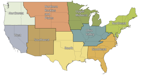
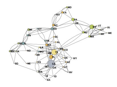
Figure 5: NOAA U.S. Climate Regions and network visualization of trade flows between states

Notes: The left panel shows the classification of U.S. states into nine climate regions, provided by the National Oceanic and Atmospheric Administration (source: https://www.ncei.noaa.gov/access/monitoring/reference-maps/us-climate-regions). Hawaii and Alaska are not considered in this classification but are kept in the analysis. The right panel displays the network visualization of the bilateral trade flows between U.S. States.

On the left panel of Figure 5 we show the nine climate regions according to the classification provided by the National Oceanic and Atmospheric Administration (Karl and Koss, , 1984). The nine climate regions are: Northeast (NE), Southeast (SE), South (S), Upper Midwest (UMW), Ohio Valley (OV), Northern Rockies and Plains (NP), Southwest (SW), West (W), and Northwest (NW).

A network representation of the interstate trade flows, instead, is provided in the right panel of Figure 5. Visual clutter is reduced using CFS data to determine, for each state, the three most important trade partners and representing the network as an undirected graph. Nodes are proportional to the size of the local economy, as proxied by state employment in 2017 sourced from the FRED-SD database (Bokun et al., , 2023), and have the same color as the climate region to which they belong, as shown in the left panel of the figure. The network reflects the underlying spatial proximity of states as well as their centrality to the U.S. economy as a whole. For instance, we can observe a cluster of northeastern economies tightly interconnected on the right portion of the graph. Moreover, it is evident that New York, Texas, Florida, and California, not only represent the largest economies in terms of employment, but are also heavily connected with several other states, thus playing a pivotal role in the entire U.S. economy.

3 A GVAR model for the U.S. economy

We construct a GVAR model for the U.S. economy by aggregating state-specific autoregressive models ($ARX^{\star}$) that include rest-of-U.S. (RoUS) exogenous variables, along with weather shocks. RoUS aggregate variables are calculated as weighted averages across all other states, using inter-state trade shares as weights. Since RoUS aggregates are treated as weakly exogenous in each $ARX^{\star}$ model, estimation can be performed at the state level, thus avoiding overparametrization problems. Let $y_{it}$ denote an indicator of economic activity for state $i$ at time $t$ (i.e. MECI), and $s_{it}$ be our state-level weather-shock proxy. For ease of notation, in the following discussion we consider a model with one lag. The $ARX^{\star}$ for state $i$ is then given by:

$$y_{it}=\alpha_{i}+\beta_{i}y_{i,t-1}+\gamma_{0i}y_{it}^{\ast}+\gamma_{1i}y_{i,t-1}^{\ast}+\theta_{i}s_{it}+u_{it}$$ (3)

where $y_{it}^{\ast}$ denotes RoUS average economic activity, $\alpha_{i}$, $\beta_{i}$, $\gamma_{0i}$, $\gamma_{1i}$ and $\theta_{i}$ are parameters to be estimated, and $u_{it}$ is an i.i.d. error with mean 0 and variance $\sigma_{i}^{2}$. As shown by Dées et al., 2007a , the GVAR can be derived as an approximation to a global unobserved common factor model, where common factors are captured by cross-country averages. In our model, cross-state averages capture factors that affect the U.S. economy as a whole, such as international demand for U.S. goods.

Let $\mathbf{W}_{i}$ denote the weight matrix for state $i$, such that:

$$\begin{pmatrix}y_{it}\\ y_{it}^{\ast}\end{pmatrix}=\mathbf{W}_{i}\begin{pmatrix}y_{1t}&y_{2t}&\bf\cdots&y_{Nt}\end{pmatrix}^{\prime}=\mathbf{W}_{i}\mathbf{y}_{t}$$ (4)

where $N=50$ is the number of states and $\mathbf{y}_{t}$ is the country-wide vector of endogenous variables. Specifically, $\mathbf{W}_{i}$ contains the weights of all states in the trade network of state $i$, measured using CFS data introduced in Section 2. As mentioned before, the weight of state $j$ in the network of state $i$ is calculated as the sum of bilateral imports and exports between $i$ and $j$ as a ratio of total trade of state $i$ with all other states in the U.S.

Stacking all $ARX^{\star}$ models, we get a country-wide model:

$$\mathbf{G}\mathbf{y}_{t}=\boldsymbol{\alpha}+\mathbf{H}\mathbf{y}_{t-1}+\boldsymbol{\Theta}\mathbf{s}_{t}+\mathbf{u}_{t}$$ (5)

where

$$\mathbf{G}=\begin{pmatrix}\left(1,-\gamma_{01}\right)\mathbf{W}_{1}\\ \left(1,-\gamma_{02}\right)\mathbf{W}_{2}\\ \vdots\\ \left(1,-\gamma_{0N}\right)\mathbf{W}_{N}\end{pmatrix}\hskip 35.0pt\mathbf{H}=\begin{pmatrix}\left(\beta_{1},\gamma_{11}\right)\mathbf{W}_{1}\\ \left(\beta_{2},\gamma_{12}\right)\mathbf{W}_{2}\\ \vdots\\ \left(\beta_{N},\gamma_{1N}\right)\mathbf{W}_{N}\end{pmatrix}\hskip 35.0pt\boldsymbol{\Theta}=\begin{pmatrix}\theta_{1}&0&\dots&0\\ 0&\theta_{2}&\dots&0\\ \vdots&\vdots&\ddots&\vdots\\ 0&0&\dots&\theta_{N}\end{pmatrix}$$ (6)

while $\boldsymbol{\alpha}$, $\mathbf{s}_{t}$ and $\mathbf{u}_{t}$ are vectors of stacked constants, weather shocks and errors, respectively. By inverting the matrix $\mathbf{G}$, we obtain a reduced-form VAR for the entire U.S. economy:

$$\mathbf{y}_{t}=\mathbf{c}+\mathbf{F}\mathbf{y}_{t-1}+\boldsymbol{\Lambda}\mathbf{s}_{t}+\boldsymbol{\varepsilon}_{t}$$ (7)

where $\mathbf{c}=\mathbf{G}^{-1}\boldsymbol{\alpha}$, $\mathbf{F}=\mathbf{G}^{-1}\mathbf{H}$, $\boldsymbol{\Lambda}=\mathbf{G}^{-1}\boldsymbol{\Theta}$, and $\boldsymbol{\varepsilon}_{t}=\mathbf{G}^{-1}\mathbf{u}_{t}$. It is important to remark that matrix $\boldsymbol{\Lambda}$ is not diagonal: its off-diagonal elements capture contemporaneous cross-border effects of weather shocks.

4 Empirical Results

We estimate our monthly GVAR from January 1990 to December 2019. We exclude the subsequent period to prevent our results from being biased by the COVID-19 pandemic. We rely on a GVAR model with 2 lags as suggested by minimization of the Bayesian information criterion, which selects at most 2 lags for almost all states. We derive our baseline results using the MECI as a measure of local economic activity. Unit root tests indicate that the level of the MECI is non-stationary or near unit root for a number of states, and stationary for others. Therefore, we transform the MECI indices by taking their first differences and estimate each ARX* model (3) by OLS.

We assess the direct and indirect macroeconomic effects of weather shocks by means of impulse response functions (IRFs) estimated on a sample that runs from April 1990 through December 2019, for a total of 357 observations (i.e. after taking first differences of MECI and considering two lags). While we carry out the impulse-response analysis at the state level, in what follows, to summarize results, we aggregate the estimated individual IRFs into those for nine U.S. climate regions, as previously shown in Figure 5. Note that while Hawaii and Alaska are not considered in this classification, we do retain them in the GVAR analysis.

When simulating a weather shock, we assume that all states in a region are contemporaneously hit. As a matter of fact, Figure 3 highlights that major weather events such as the Storm of the Century in 1993, the Blizzard of 1996, Hurricane Katrina in 2005 and the Super Outbreak in 2011 have triggered emergency declarations in a very large portion of the U.S. This is thus an extremely adverse but realistic scenario, that allows us to interpret the results as “upper bound” of cross-regional spillover effects.

4.1 Main results

We assess the responses of MECI to a region-wide weather shock in Figures 6 and 7. While GVAR models are estimated using the first differences of MECI, we cumulate the Impulse Response Functions (IRFs) to obtain the level responses of the index that is scaled to match the four-quarter percent growth rate of U.S. GDP. Figure 6 shows the IRFs for a subset of regions (i.e. NE, SE, S, and W), while Figure 7 reports the IRFs for all regions one year after shock, which seems a reasonable time frame to assess magnitude of macroeconomic effects induced by weather disasters. We compute means and the corresponding 10th and 90th percentile using a bootstrap procedure for GVAR models (see Dées et al., 2007a, ; Dées et al., 2007b, , for details).

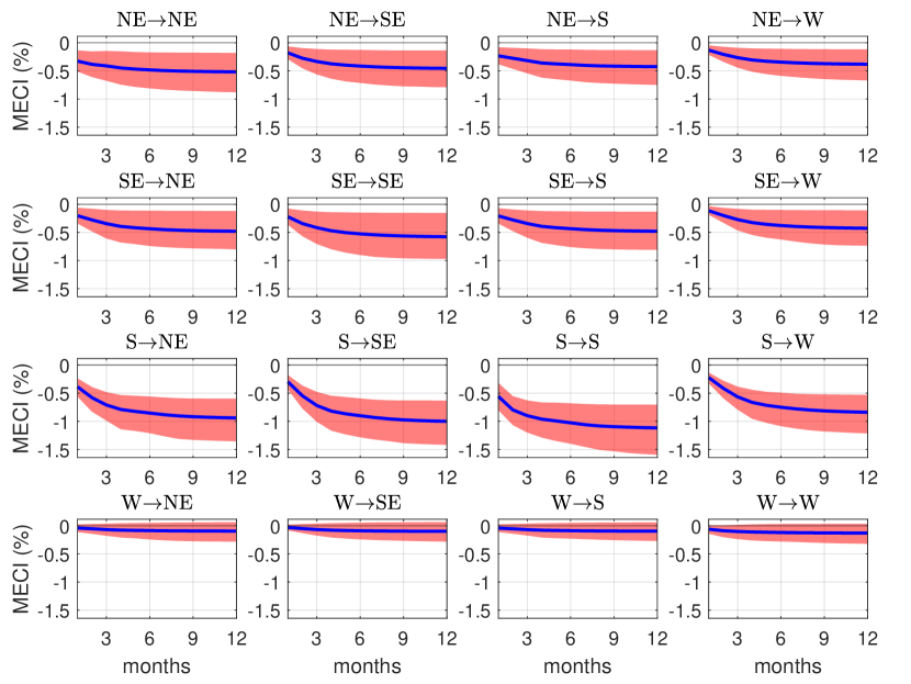
Figure 6: Impulse response functions - Monthly Economic Conditions Indicators

Notes: Responses of the Monthly Economic Conditions Indicator (MECI) to a weather shock hitting 100% of counties in the shocked region. The horizontal axis shows months, the vertical axis the responses in percentage points. Blue solid lines indicate bootstrap means and the red area the corresponding 10th and 90th percentile. Four climate regions are considered: Northeast (NE), Southeast (SE), South (S), and West (W). In titles, the first region indicates where the shock originates, while the second one is where it propagates.

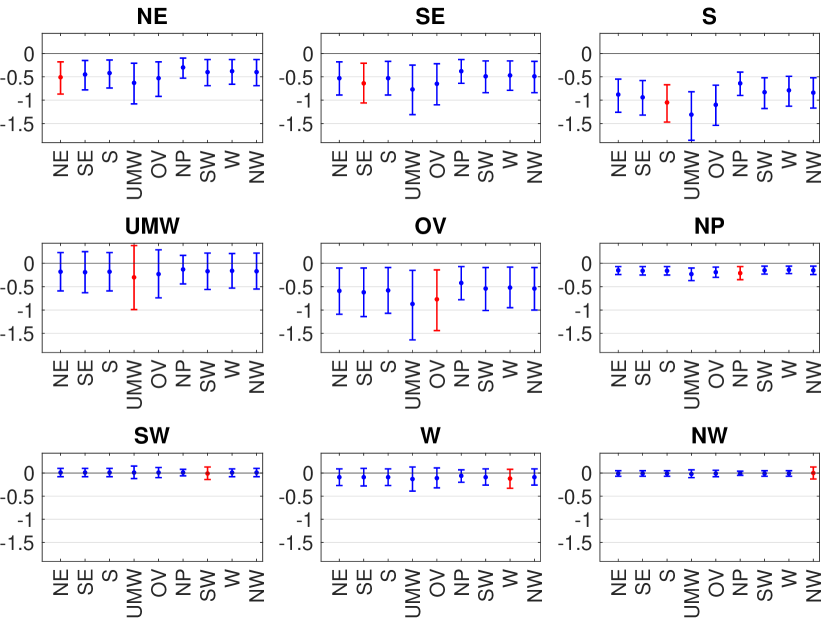
Figure 7: IRFs of Monthly Economic Conditions Indicators at 12-month horizon

Notes: The figure displays IRF bootstrap means along with their corresponding 10th and 90th percentile. The regions affected by shocks are specified on the x-axis, while the title identifies the origin of the shocks.

Remarkably, responses of real economic activity are generally negative, both within the shocked region and in regions not directly affected by the weather shock. Except for Western regions (W, NW, and SW), all regions generate significant spillovers. The IRFs generally converge within approximately one year after the shock. Because of the unit roots/near unit-root behavior of MECI, the model predicts permanent effects, but these may be simply considered as approximations of highly persistent effects, in line with the findings of previous literature on the effects of extreme climatic events (Batten, , 2018; Hsiang and Jina, , 2014).

Figure 7 reports the mean bootstrap response with the corresponding 10th and 90th percentile one year after the shock. The largest spillovers (in absolute values) are generated by the South (S), Southeast (SE) and Ohio Valley (OV) regions. Concerning the magnitude of the effects, the mean responses after one year are generally in the range from -1.3 to 0. This indicates, approximately, a drop of up to 1.3% in year-on-year growth rates of economic activity, in response to the region-wide weather shock. The single largest IRFs (in absolute values) is represented by the response of the Upper Midwest (UMW) region to a weather shock in the South (S).

4.2 The role of economic linkages and spatial adjacency

The GVAR model allows to estimate spillover effects, taking into account the economic interdependence between states. In this section, we assess the importance of explicitly considering economic linkages using interstate trade flows. To this aim, we re-estimate the GVAR model using alternative weight matrices $\mathbf{W}_{i}$ based on spatial adjacency.

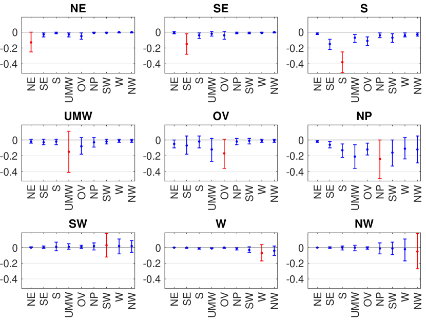
Figure 8: IRFs using spatial adjacency matrix, 12-month horizon

Notes: see notes to Figure 7.

Figure 8 reports the IRFs of MECI calculated based on geographical proximity. Cross-region effects of weather shocks are almost entirely wiped out, and intra-regional effects are substantially reduced, relative to the baseline results in Figure 7.

4.3 The role of parameter heterogeneity and disaggregation

A spatial dynamic model. In the GVAR specification parameters are heterogeneous across states. To highlight the importance of such heterogeneity, we compare the baseline GVAR results with the estimates of a spatial dynamic model (i.e., a model with both space and time lags), in which all states share the same parameters:

$$y_{it}=p\tilde{W_{i}}y_{it}+\gamma y_{i,t-1}+\rho\tilde{W_{i}}y_{i,t-1}+\beta s_{it}+c_{i}+e_{it}$$ (8)

where $\tilde{W_{i}}$ is a $N$-dimensional vector of trade weights, $p,\gamma,\rho,\beta$ are parameters, $c_{i}$ denotes state fixed effects and $e_{it}$ is the error term. We use a tilde to distinguish the vector of weights on which we rely here from the $2\times N$ matrix used in (4), but the bilateral weights are exactly the same in the two models. Yu et al., (2008) have developed quasi-maximum likelihood estimators for spatial dynamic panel models of the form (8). In Panel (a) of Table 1, we report bias-corrected estimates of model (8), using 1000 iterations of the Yu et al., (2008) algorithm. The coefficient on weather shocks is around $-0.073$ and statistically distinguishable from zero.

Table 1: The role of parameter heterogeneity and disaggregation

(a) A spatial dynamic model
variable	coefficient	std. error
$\tilde{W_{i}}y_{it}$	0.6910***	0.0094
$y_{i,t-1}$	0.1586***	0.0074
$\tilde{W_{i}}y_{i,t-1}$	-0.0309***	0.0119
$s_{it}$	-0.0734***	0.0099
(b) An aggregate U.S. ARDL model
variable	coefficient	std. error
$y_{t-1}$	0.6037***	0.0529
$y_{t-2}$	0.0811	0.0530
$s_{t}$	-0.2255	0.1572
$const$	0.0083	0.0118

(c) Heterogeneous coefficients of $s_{it}$ in the GVAR
parameter	average	std. dev.	min	max
$\theta_{i}$	$-0.066$	$0.11$	$-0.61$	$0.065$

Notes: Panel (a) reports estimates of a spatial dynamic panel model. The estimates of an autoregressive distributed lag (ARDL) model for the aggregate U.S. economy are shown in panel (b). Panel (c) displays the average point estimate of coefficient $\theta_{i}$ (i.e. the impact effect of weather shocks) across the state-specific ARX* models (3) composing the GVAR, along with the standard deviation of the estimates across states, and the minimum and the maximum estimates. In panels (a) and (b), ^∗∗∗ indicates 1% significance, the other coefficients in panel (b) are not significant at the 10% level.

A country-wide regression for the U.S. Next, we consider a model that does not feature geographical disaggregation. Specifically, we estimate an autoregressive distributed lag model (ARDL) for the aggregate U.S. economy at the monthly frequency. As shown in Panel (b) of Table 1, the effect of weather shocks is negative but statistically indistinguishable from zero. We conclude that disaggregation matters, when it comes to estimating the economic impact of weather events.

Finally, for comparison, panel (c) of Table 1 reports the average point estimate of the impact effect of weather shocks, $\theta_{i}$, across the state-specific ARX* models (3) composing the GVAR, along with the standard deviation of the estimates across states, the minimum and the maximum estimates. The average estimate of $\theta_{i}$ in the GVAR model ($-0.066$) is similar to the coefficient on weather shocks in the spatial dynamic model ($-0.073$). However, the dynamic panel model fails to capture the heterogeneity of the response to weather shocks across states. As highlighted in panel (c), the estimated effects of weather shocks vary substantially across states in the GVAR model: the point estimates of coefficient $\theta_{i}$ have a standard deviation of $0.11$ across states, with values in the range from $-0.61$ to $0.065$ (for Louisiana and Maine, respectively).

4.4 The economic effects of specific weather related disasters

The adverse weather conditions during winter and tropical storms - hurricanes in particular - are often the headline news due to their severe impacts on economic activity and supply chains. We thus focus on disasters triggered by such weather shocks in the climate regions where they happens more often.

In the case of shocks associated with adverse winter weather conditions, these are concentrated in the Northeast, Ohio Valley, and Southeast regions. As shown in the upper panel of Figure 9, shocks originating in any of these regions have significant negative impacts in all of the other regions. We can note that the Upper Midwest is particularly affected by shocks originating in the Northeast, Ohio Valley, and Southeast regions. This can be rationalized by looking at Figure 5, which shows that these regions are not only geographically close but also economically tightly linked through trade flows to the Upper Midwest.

As for shocks triggered by tropical storms, these are concentrated in the Northeast, Southeast, and South of the U.S. The lower panel of Figure 9 highlights that in this case only shocks originating in the South of the U.S. have negative and statistically significant impacts on the rest of the U.S. The magnitude of the response is larger for the neighboring regions and for the Northeast and the Upper Midwest than for western regions. This can be in part explained by the fact that the single most disruptive weather event in the recent history of the U.S. – Hurricane Katrina – has impacted the South of the country.

Figure 9: IRFs of Monthly Economic Conditions Indicators at 12-month horizon: Winter Weather and Tropical storms

(a) Winter Weather

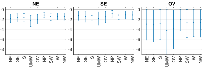
(b) Tropical Storms

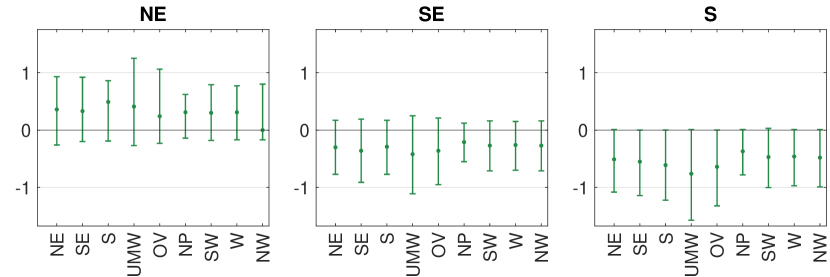
Notes: see notes to Figure 7.

4.5 Indirect effects of weather shocks on local activity

To quantify indirect effects of weather shocks on local activity for each state, we compare the IRFs derived from the GVAR model with alternative IRFs derived using state-specific ARDL ($ARX^{\star}$) models and assuming that RoUS variables are not affected by changes in state-specific variables. The difference between the IRFs in the two cases capture “second-round effects”: a weather shock in state $i$ causes economic adjustment in the other states, which in turn feeds back into state $i$.

Figure 10 isolates second-round effects by comparing GVAR and ARDL estimates of the response of MECI to a weather shock after a year. In absolute terms and independently of the model being used, these effects are especially strong in Louisiana (LA) and Illinois (IL). While the first response is chiefly driven by the impact of Hurricane Katrina in 2005, the second is associated with the Great Flood of 1993, which caused one of the most extensive financial losses and widespread devastation in modern U.S. history. More generally, we note that, as expected, GVAR estimates have wider confidence intervals but also tend to be greater in absolute value, hence reinforcing the conclusion that spillovers do matter in assessing the impacts of weather shocks. As a back-of-the-envelope calculation, the legend of the figure indicates that in absolute terms, both the average and median responses from the GVAR are larger than those from the ARDL model.

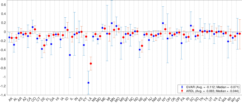
Figure 10: Second-round effects of weather shocks

Notes: For each state, the figure reports the point estimates of 12-month-ahead responses of state-level MECI to a simulated weather shock in the same state, provided by the U.S. GVAR model (blue squares) and by state-specific ARDL ($ARX^{\ast}$) models in which the rest of the U.S. economy is exogenous (red circles). The bars denote the 10% and 90% percentile from the bootstrap distribution.

5 Conclusions

We have investigated the effects of weather shocks on economic activity across U.S. states, with a particular focus on cross-border spillover effects. Using a GVAR framework, we have shown that severe weather shocks generally cause drops in state-level economic activity, with negative effects propagating to other regions through economic linkages between states. We estimate that an extreme weather event involving one climate region of the U.S. has the potential to reduce regional yearly growth rates by up to 1.3 percentage points, approximately. Because of indirect (second-round) effects, network relationships between states amplify the total impact that weather shocks have on the states where they occur.

References

- Ahmadi et al., (2022) Ahmadi, M., Casoli, C., Manera, M., and Valenti, D. (2022). Modelling the effects of climate change on economic growth: A Bayesian structural global vector autoregressive approach. Working Papers 2022.46, Fondazione Eni Enrico Mattei.
- Baker and Bloom, (2013) Baker, S. R. and Bloom, N. (2013). Does uncertainty reduce growth? Using disasters as natural experiments. NBER Working Paper 19475, National Bureau of Economic Research.
- Barro, (2006) Barro, R. J. (2006). Rare disasters and asset markets in the twentieth century. Quarterly Journal of Economics, 121(3):823–866.
- Barrot and Sauvagnat, (2016) Barrot, J.-N. and Sauvagnat, J. (2016). Input specificity and the propagation of idiosyncratic shocks in production networks. The Quarterly Journal of Economics, 131(3):1543–1592.
- Batten, (2018) Batten, S. (2018). Climate change and the macro-economy: A critical review. Bank of England working papers 706, Bank of England.
- Baumeister et al., (2022) Baumeister, C., Leiva-León, D., and Sims, E. (2022). Tracking weekly state-level economic conditions. The Review of Economics and Statistics, pages 1–45.
- Benzie, (2021) Benzie, M. (2021). Cross-border climate change impacts: Implications for the European Union. Regional Environmental Change, 19:763–776.
- Billio et al., (2020) Billio, M., Casarin, R., Cian, E. D., Mistry, M., and Osuntuyi, A. (2020). The impact of climate on economic and financial cycles: A markov-switching panel approach. Technical report, arXiv preprint arXiv:2012.14693.
- Bloesch and Gourio, (2015) Bloesch, J. and Gourio, F. (2015). The effect of winter weather on U.S. economic activity. Economic Perspectives, 39(1):1–20.
- Boehm et al., (2019) Boehm, C. E., Flaaen, A., and Pandalai-Nayar, N. (2019). Input linkages and the transmission of shocks: Firm-level evidence from the 2011 Tōhoku earthquake. The Review of Economics and Statistics, 101(1):60–75.
- Bokun et al., (2023) Bokun, K. O., Jackson, L. E., Kliesen, K. L., and Owyang, M. T. (2023). FRED-SD: A real-time database for state-level data with forecasting applications. International Journal of Forecasting, 39(1):279–297.
- Boldin and Wright, (2015) Boldin, M. and Wright, J. H. (2015). Weather-adjusting economic data. Brookings Papers on Economic Activity, Fall:227–260.
- Burke et al., (2015) Burke, M., Hsiang, S. M., and Miguel, E. (2015). Global non-linear effect of temperature on economic production. Nature, 527(7577):235–239.
- Carter et al., (2021) Carter, T. R., Benzie, M., Campiglio, E., Carlsen, H., Fronzek, S., Hildén, M., Reyer, C. P., and West, C. (2021). A conceptual framework for cross-border impacts of climate change. Global Environmental Change, 69:102307.
- Carvalho et al., (2020) Carvalho, V. M., Nirei, M., Saito, Y. U., and Tahbaz-Salehi, A. (2020). Supply Chain Disruptions: Evidence from the Great East Japan Earthquake. The Quarterly Journal of Economics, 136(2):1255–1321.
- Cashin et al., (2017) Cashin, P., Mohaddes, K., and Raissi, M. (2017). Fair weather or foul? The macroeconomic effects of El Niño. Journal of International Economics, 106:37–54.
- Cavallo et al., (2013) Cavallo, E., Galiani, S., Noy, I., and Pantano, J. (2013). Catastrophic natural disasters and economic growth. Review of Economics and Statistics, 95(5):1549–1561.
- Colacito et al., (2019) Colacito, R., Hoffmann, B., and Phan, T. (2019). Temperature and growth: A panel analysis of the United States. Journal of Money, Credit and Banking, 51(2-3):313–368.
- Colombo and Ferrara, (2024) Colombo, D. and Ferrara, L. (2024). Dynamic effects of weather shocks on production in European economies. CAMA Working Papers 2024-07, Centre for Applied Macroeconomic Analysis, Crawford School of Public Policy, The Australian National University.
- Dell et al., (2014) Dell, M., Jones, B. F., and Olken, B. A. (2014). What do we learn from the weather? The new climate-economy literature. Journal of Economic Literature, 52(3):740–798.
- (21) Dées, S., di Mauro, F., Pesaran, M. H., and Smith, L. V. (2007a). Exploring the international linkages of the euro area: A global VAR analysis. Journal of Applied Econometrics, 22(1):1–38.
- (22) Dées, S., Holly, S., Pesaran, M. H., and Smith, L. V. (2007b). Long run macroeconomic relations in the global economy. Economics - The Open-Access, Open-Assessment E-Journal, 3:1–20.
- Feng et al., (2023) Feng, A., Li, H., and Wang, Y. (2023). We are all in the same boat: Cross-border spillovers of climate shocks through international trade and supply chain. CESifo Working Paper Series 10402, CESifo.
- Forslid and Sanctuary, (2023) Forslid, R. and Sanctuary, M. (2023). Climate risks and global value chains: The impact of the 2011 Thailand flood on Swedish firms. CEPR Discussion Papers 17855, C.E.P.R. Discussion Papers.
- Gourio, (2012) Gourio, F. (2012). Disaster risk and business cycles. American Economic Review, 102(6):2734–66.
- Hsiang, (2016) Hsiang, S. (2016). Climate econometrics. Annual Review of Resource Economics, 8(1):43–75.
- Hsiang and Jina, (2014) Hsiang, S. M. and Jina, A. S. (2014). The causal effect of environmental catastrophe on long-run economic growth: Evidence from 6,700 cyclones. NBER Working Papers 20352, National Bureau of Economic Research, Inc.
- IPCC, (2023) IPCC (2023). Weather and climate extreme events in a changing climate, page 1513–1766. Cambridge University Press.
- Kahn et al., (2021) Kahn, M. E., Mohaddes, K., Ng, R. N., Pesaran, M. H., Raissi, M., and Yang, J.-C. (2021). Long-term macroeconomic effects of climate change: A cross-country analysis. Energy Economics, 104:105624.
- Karl and Koss, (1984) Karl, T. and Koss, W. J. (1984). Regional and national monthly, seasonal, and annual temperature weighted by area, 1895-1983. Technical Report 3-4, National Climatic Data Center.
- Kashiwagi et al., (2021) Kashiwagi, Y., Todo, Y., and Matous, P. (2021). Propagation of economic shocks through global supply chains—evidence from Hurricane Sandy. Review of International Economics, 29(5):1186–1220.
- Kim et al., (2021) Kim, H. S., Matthes, C., and Phan, T. (2021). Extreme weather and the macroeconomy. Working Paper 21-14, Federal Reserve Bank of Richmond.
- Mohaddes et al., (2022) Mohaddes, K., Ng, R. N. C., Pesaran, M. H., Raissi, M., and Yang, J.-C. (2022). Climate change and economic activity: Evidence from U.S. states. Oxford Open Economics, 2:odac010.
- Natoli, (2023) Natoli, F. (2023). The macroeconomic effects of temperature surprise shocks. Technical Report 1407, Bank of Italy.
- NOOA, National Centers for Environmental Information, (2018) NOOA, National Centers for Environmental Information (2018). U.S. Billion-Dollar Weather and Climate Disasters. https://www.ncdc.noaa.gov/billions/, accessed April 7, 2018.
- Pesaran et al., (2004) Pesaran, M. H., Schuermann, T., and Weiner, S. M. (2004). Modeling regional interdependencies using a global error correcting macroeconometric model. Journal of Business and Economic Statistics, 22(2):129–62.
- Ramey, (2016) Ramey, V. (2016). Macroeconomic shocks and their propagation. In Taylor, J. B. and Uhlig, H., editors, Handbook of Macroeconomics, volume 2, chapter 0, pages 71–162. Elsevier.
- Strömberg, (2007) Strömberg, D. (2007). Natural disasters, economic development, and humanitarian aid. Journal of Economic Perspectives, 21(3):199–222.
- Tran and Wilson, (2020) Tran, B. R. and Wilson, D. J. (2020). The local economic impact of natural disasters. Working Paper Series 2020-34, Federal Reserve Bank of San Francisco.
- van der List and Wilson, (2016) van der List, C. and Wilson, D. J. (2016). Clearing the fog: The effects of weather on jobs. FRBSF Economic Letter, 2016-29.
- Wilson, (2016) Wilson, D. J. (2016). The impact of weather on local employment: Using big data on small places. Working Paper Series 2016-21, Federal Reserve Bank of San Francisco.
- Yu et al., (2008) Yu, J., de Jong, R., and fei Lee, L. (2008). Quasi-maximum likelihood estimators for spatial dynamic panel data with fixed effects when both N and T are large. Journal of Econometrics, 146(1):118–134.