[1,2]\fnmJorge-Humberto \surUrrea-Quintero
[3]\fnmMichele \surMarino
[4]\fnmThomas \surWick
[1]\fnmUdo \surNackenhorst
1]\orgnameLeibniz University Hannover, \orgdivIBNM - Institute of Mechanics and Computational Mechanics, \orgaddress\streetAppelstraße 9a, \cityHannover, \postcode30167, \stateLower Saxony, \countryGermany
2]\orgnameTechnische Universtität Braunschweig, \orgdiviRMB - Institute for Computational Modeling in Civil Engineering, \orgaddress\streetPockelsstr. 3, \cityBraunschweig, \postcode38106, \stateLower Saxony, \countryGermany
3]\orgdivDepartment of Civil Engineering and Computer Science Engineering, \orgnameUniversity of Rome Tor Vergata, \orgaddress\streetVia del Politecnico 1, \cityRome, \postcode00133, \countryItaly
4]\orgnameLeibniz University Hannover, \orgdivInstitut für Angewandte Mathematik, \orgaddress\streetWelfengarten 1, \cityHannover, \postcode30167, \stateLower Saxony, \countryGermany
A comparative analysis of transient finite-strain coupled diffusion-deformation theories for hydrogels
Abstract
This work presents a comparative review and classification between some well-known thermodynamically consistent models of hydrogel behavior in a large deformation setting, specifically focusing on solvent absorption/desorption and its impact on mechanical deformation and network swelling. The proposed discussion addresses formulation aspects, general mathematical classification of the governing equations, and numerical implementation issues based on the finite element method. The theories are presented in a unified framework demonstrating that, despite not being evident in some cases, all of them follow equivalent thermodynamic arguments. A detailed numerical analysis is carried out where Taylor-Hood elements are employed in the spatial discretization to satisfy the inf-sup condition and to prevent spurious numerical oscillations. The resulting discrete problems are solved using the FEniCS platform through consistent variational formulations, employing both monolithic and staggered approaches. We conduct benchmark tests on various hydrogel structures, demonstrating that major differences arise from the chosen volumetric response of the hydrogel. The significance of this choice is frequently underestimated in the state-of-the-art literature but has been shown to have substantial implications on the resulting hydrogel behavior.
keywords:
hydrogels, finite element method, thermodynamic consistency, mathematical classification, large deformations, nonlinear coupled problems, FEniCS.1 Introduction
Hydrogels, a class of versatile soft materials with the unique ability to absorb and retain fluid within their three-dimensional network structures, have gained widespread attention in recent years across various industrial applications. Their diverse uses include serving as drug carriers in biomedical applications [43, 27], absorbents of pollutants in agriculture [27], and smart sensors or actuators in engineering [10, 32]. These properties can be fine-tuned by manipulating chemical composition, crosslinking density, and fluid content [9]. In this work, we aim to provide an in-depth examination of diffusion-deformation hydrogel theories and the implications of selecting underlying constitutive theory in the large deformation setting.
Several comprehensive reviews have emerged in the study of hydrogels, discussing topics ranging from hydrogel deformation theories to the microstructural impact on mechanical behaviors. [36] provided an exhaustive review of hydrogel deformation theories, blending both theoretical analyses and practical applications, emphasizing mechanics’ role. [26] delve into advances in constitutive models for hydrogels and shape memory polymers (SMPs), categorizing six primary hydrogel types and highlighting potential hyperelastic model adaptations. Meanwhile, [30] offered insights into hydrogel network models, discussing the microstructural impact on their mechanical behaviors like swelling, elasticity, and fracture. This research underscores the potential synergy between network modeling and continuum mechanics in capturing hydrogel dynamics.
Modeling the diffusion-deformation process in hydrogels necessitates a comprehensive understanding of the material’s behavior during swelling and mechanical deformation. This understanding hinges on a mathematical formulation that simultaneously accounts for the diffusion of fluid molecules within the hydrogel’s polymer network and the corresponding mechanical deformations induced by swelling. Two primary approaches can be employed to describe these phenomena: mixture theories and macro-scale theories. Mixture theories, representing the porous medium as spatially superimposed interacting layers [18], often involve a complex array of model parameters and constitutive choices, making them challenging to calibrate in practical applications. Consequently, this paper focuses on macro-scale poroelastic theories, which view the medium as a homogenous material characterized by a coupled deformation-diffusion response, as developed in the seminal works by Biot [e.g., 3]. Within this framework, the key equations, such as the mass balance and mechanical equilibrium equations, govern both the conservation of mass and the balance of forces within the hydrogel. An appropriate chemo-mechanical constitutive description for the macroscopic continuum completes the modeling framework. Constitutive laws couple the mechanical response of the polymer network (accounting, for example, for hyperelastic or viscoelastic effects) with changes in fluid distribution within the hydrogel mesh, describing mixing effects and the interaction between diffusion and deformation.
Over the years, various models have been developed to describe coupled diffusion-deformation effects in elastomeric gels. These models couple a common general poroelastic framework with the effects of different physical fields, resulting in a wide range of stimuli-based responses encountered in various applications. Regarding the general poroelastic framework, for instance, [25] and [49] provided a continuum mechanics framework, as well as analytical and finite element solutions, of the coupled problem in the large deformation setting. [12] provided a comprehensive thermodynamics-consistent formulation of the diffusion-deformation theory under isothermal conditions. In contrast, [38] benchmarked the diffusion-deformation theory against some experiments involving localized exposure of the gel boundary to a solvent, where large bending deformations appear during solvent absorption. With respect to more complex stimuli-based responses, [13] extended the theory and accounted for temperature effects as well. [14] summarized the main developments of the thermo-mechanically coupled theory for fluid permeation in elastomeric materials and provided an open-access Abaqus implementation to simulate hydrogel’s response in 3D.
A shared mathematical characteristic of these models is the saddle point structure of the underlying variational formulation. As a result of the finite element implementations, the Ladyzhenskaya-Babuska-Brezzi (LBB), i.e., discrete inf-sup, condition might be violated, requiring equilibrated inf-sup stable finite element spaces. Otherwise, oscillatory distributions of chemical potential as the primary variable controlling species diffusion arise. These challenges can be addressed in several ways. To name a few of these approaches, in [7], an in-depth analysis of Taylor-Hood elements (see, e.g., [20]) for gel modeling is provided, while [29] proposed an enhanced assumed strain (EAS) method for the coupled problem. [4] proposed a minimization formulation for the coupled diffusion-deformation problem of polymeric hydrogels at large strains and compared this variational framework to classical saddle point-based structures. Large volume changes with instability patterns in the presence of geometrical constraints were successfully modeled. [44] developed a numerical platform to simulate the dynamic behaviors of responsive gels. The authors of this study addressed some of the challenges that were not previously resolved, such as how to handle time-dependent and coupled mass diffusion and deformation fields in a very short time, as well as numerical instability issues.
Overall, there is no consensus on formulating a constitutive model for hydrogels and its numerical implementation. This study emphasizes the essential building blocks found in common across various hydrogel theories, mainly focusing on the standard poroelastic description. It is unclear whether the underlying constitutive choices at the free energy level are equivalent. The significance of fundamental choices in coupling diffusion and deformation is frequently overlooked. For example, such choices may relate to whether volume changes in the hydrogel are solely attributed to fluid content or involve elastic mechanisms as well. In the latter scenario, the detailed description of the volumetric response plays a crucial role. We aim to analyze the impact of such assumptions on the constitutive model.
Not only do these fundamental constitutive choices lead to differences in the observed physical response, but they also influence the feasibility and appropriateness of different numerical solutions. Some theories lend themselves to a monolithic implementation of the coupled problem, while others favor a staggered approach. Despite their importance, these considerations have been largely neglected in existing literature.
1.1 General goals
This paper reviews some of the most notable models that describe the diffusion-deformation process of elastomeric gels. The models were selected based on their consistency with thermodynamic principles, their ability to represent different behaviors, and the easiness to reproduce the results using the open-source computing platform FEniCS [2], serving as a benchmark for future studies. We provide a common mathematical framework and classifications from which both staggered and monolithic numerical algorithms are derived for studying the diffusion-deformation behavior of hydrogels despite their various derivation methods. We carefully examine the distinctions and similarities between different constitutive equations and analyze their impact on the deformation of hydrogels and the evolution of associated fields through simulations. This lays the foundation for future theoretical extensions, including additional mechanisms such as chemical reactions, degradation, or damage.
1.2 Open science context
Traditionally, researchers have relied on custom numerical solvers or commercial software like Abaqus or COMSOL. While [14] made their Abaqus code publicly available, a recent push has been towards open-source platforms for addressing coupled multiphysics models. Emerging software libraries such as deal.II111https://www.dealii.org/, OpenFOAM222https://www.openfoam.com/, MOOSE333https://mooseframework.inl.gov/, and FEniCS444https://fenicsproject.org/ exemplify this trend, signaling a shift in the way researchers approach the complex challenges of modeling hydrogels.
Unlike commercial software packages, open-source projects, like FEniCS, generally allow the user to have a direct hand in implementing the problem statement, the discretization, the numerical solution, and specific manipulations since all instances can be accessed. To this end, more information about the mathematical-numerical classification and design of algorithms is required. While this provides an advantage, granting users more liberty to develop and test novel numerical algorithms and discretizations, it also constitutes a challenge. The need for more hands-on implementation and debugging is time-consuming.
To include readerships interested in open-source software and as part of the broader scope of our paper, we establish mathematical classifications to derive numerical algorithms for the coupled problem, enabling the precise study of well-posedness and facilitating rigorous numerical analysis. This includes introducing inf-sup stable Taylor-Hood finite elements for spatial discretization and using a strongly -stable, first-order, implicit Euler scheme for temporal discretization. These technical developments are summarized into compact mathematical formulations that serve as the starting point for our FEniCS implementation, allowing for meticulous examination of the numerical algorithms.
1.3 Main contributions and paper outline
The main contributions of this paper are summarized as follows:
-
1.
Unification in the formulation and notation of some representative diffusion-deformation theories applied to the large deformation of hydrogels.
-
2.
Mathematical classification and subsequent derivation and computational comparison of monolithic and staggered numerical solutions accuracy in a variational setting using the finite element method (FEM).
-
3.
One- to three-dimensional numerical simulations of well-known prototype problems to study the theories’ capabilities and robustness of the FEM implementation.
-
4.
Comparison of the different constitutive models in a single benchmark problem highlighting their main characteristics.
The paper is organized as follows. Section 2 provides a common background knowledge of gels and the basic formulations of the chosen theories using a unified notation. Section 3 is devoted to the mathematical classification and numerical approximation using the FEM in variational settings. Section 4 explains the general setting of the numerical simulations campaign. Section 5 presents the simulation results for some well-known prototype problems of the diffusion-deformation of hydrogels. Section 6 presents a unified benchmark problem for the diffusion-deformation of hydrogels. Concluding remarks are given in Section 7.
2 Nonlinear theory for the diffusion-deformation of elastomeric gels
In this section, we summarize some of the well-known theories describing the diffusion-deformation mechanisms in elastomeric gels that undergo large deformations under isothermal conditions.
As notation rules, we denote gradient in the reference and current configuration by and , respectively, whereas the divergence in the reference and current configuration is denoted by and , respectively. The time derivative of any field is denoted by . The operator refers to the trace of the second-order tensor . We denote the spatial dimension with , and in this paper, we exclusively work with . Finally, let be the time interval with end time value and its closure.
2.1 Kinematics of the deformation
Consider a continuum homogeneous elastomeric body living in the Euclidean space and its boundary . Here, denotes the displacement boundary (Dirichlet), the traction boundary (Neumann), the fluid concentration-related boundary (Dirichlet), and the fluid flux boundary (Neumann). The outward normal vector to the domain boundaries in the reference configuration is denoted by . The current configuration of this homogeneous body at any instant of time can be described by a one-to-one transformation mapping , where refers to the reference configuration. In principle, selecting any state as the reference state (e.g., the stress-free dry gel) is possible. For convenience, authors have also chosen to define the initial state as an isotropically swollen configuration from the dry state, leading to better reproduction of experimental conditions [6, 24].
The position vector in the reference configuration is related to the one in the current configuration by . The displacement field reads . The transformation map can be described in terms of the deformation gradient,
| (1) |
with , the determinant, representing the volume change of a volume element from the reference () to the current () configuration, and being the identity tensor.
As is standard,
| (2) | ||||
| (3) |
denote the right and left Cauchy-Green tensors, respectively. Additionally, the first invariant of is given by
| (4) |
2.1.1 Chemical potential and swelling deformation
The solvent component of the hydrogel is described by introducing its chemical potential , that is, the energy absorbed or released due to a change in its content. Fluid absorption/desorption is kinematically described through an inelastic part of the deformation . The volume change associated with fluid absorption/desorption is linked with the referential fluid concentration variable , i.e., the number of absorbed fluid molecules per unit volume of the reference configuration, by enforcing:
| (5) |
where denotes the volume of a mole of fluid molecules. This relationship can also be equivalently described by introducing the polymer volume fraction variable , defined as:
| (6) |
resulting . The dry state of the gel corresponds to , and represents a swollen state.
A generally adopted choice is to assume an isotropic swelling deformation , hence reading as:
| (7) |
where represents the polymer network stretch due to swelling. It is noteworthy that, since by definition, it results in .
2.1.2 Elastic deformation
The total deformation of a hydrogel is obtained from the superimposition of the fluid-related deformation gradient and the elastic one . The latter originates from the effects of mechanical actions to restore compatibility. Based on the previously introduced choices, we obtain:
| (8) |
At this standpoint, depending on the volume change associated with the elastic deformation , a general classification between two classes of models is introduced:
-
1.
elastic compressible models (non-constrained formulations). In this case, the elastic part of the deformation is assumed to be compressible. It is then allowed ;
-
2.
elastic incompressible models (constrained formulations). In this case, the elastic part of the deformation is assumed to be perfectly incompressible, and the total volume change of the hydrogel is related only to fluid volume changes. In other words, it results in and the kinematic constraint,
(9) has to be enforced within the theoretical formulation.
2.2 Governing partial differential equations
The two governing partial differential equations (PDEs) for the vector-valued displacements and scalar-valued, time-dependent, fluid content in terms of the concentration when expressed in the reference configuration, consist of:
-
1.
The local form of the balance of linear momentum reads:
(10) Here, denotes the first Piola-Kirchhoff stress tensor, and its initial value at . An alternative stress measure also commonly employed is the Cauchy stress tensor . External actions consist of body forces per unit deformed volume in the reference configuration . Moreover, boundary conditions prescribe displacement and traction on separate portions of the boundary. Notice that inertial effects have been neglected due to the considerably slow dynamics of the fluid diffusion evolution w.r.t. the time scale of the wave propagation.
-
2.
The local form of the mass balance of fluid content inside the hydrogel reads:
(11) Here, is the fluid flux vector in the reference configuration, related to the one in the current configuration via . Boundary conditions prescribe values of chemical potential and fluid flux in the reference configuration on the boundaries. Moreover, refers to the initial value of the chemical potential inside the hydrogel. Notice that the mass balance of fluid content is written in terms of and , but its corresponding boundary and initial conditions involve a different variable, the chemical potential . The connection of equation (11) with becomes clear by introducing a constitutive relation for , e.g., through Fick’s laws of diffusion.
2.3 Constitutive equations: stress and chemical potential
This section introduces constitutive equations for the stress and chemical potential, addressing both compressible or perfectly incompressible formulations.
2.3.1 Compressible formulations
Following standard thermodynamic arguments [48, 21, 12, 13], the local form of the second law of thermodynamics reads:
| (12) |
where is the free energy density function (per unit reference volume). Guided by equation (12), the free energy density function can be regarded as a function of the total deformation and fluid concentration , that is:
| (13) |
Consequently, equation (12) can be reformulated as:
| (14) |
and the following thermodynamically-consistent constitutive relations can be established for the first Piola-Kirchhoff stress tensor (PK1):
| (15) |
and for the chemical potential:
| (16) |
Alternative formulations can be found in the state-of-the-art for defining stresses and chemical potential, built upon elastic stress and active chemical potential concepts. These are reviewed and discussed in appendix A, showing that both approaches lead to identical results.
2.3.2 Incompressible formulations
Incompressible models require a special treatment of the kinematic constraint in equation (9) that has to be satisfied a priori within the formulation. A first possibility is to extend the free energy in equation (13) in the context of Lagrangian formulations by introducing a constrained free-energy that reads:
| (17) |
where represents a pressure-like Lagrange multiplier to enforce the kinematic constraint in equation (9) through a variational framework. By replacing with , equation (14) reads:
| (18) |
since and . From equation (18), the following thermodynamically consistent choices can be introduced for the first Piola-Kirchhoff stress tensor:
| (19) |
and for the chemical potential:
| (20) |
Such an approach has been followed, for instance, by [6, 12].
Alternatively, the kinematic constraint in equation (9) can be embedded directly within the free-energy function. For instance, this rationale is described and adopted by [33, 34]. In this case, the fluid concentration is regarded as a dependent variable since it is related to the deformation gradient (or displacements ) through equation (9). Hence, the free energy can be reformulated in the form:
| (21) |
Then, equation (14) reads:
| (22) |
since from the incompressibility constraint. From equation (22) and noting that , the first Piola-Kirchhoff stress tensor can be expressed as:
| (23) |
As previously noted, the fluid concentration can no longer be considered as an independent variable. Therefore, the chemical potential shall now be considered as the problem’s primary variable. Consequently, a special treatment is required for the term in the mass balance equation (28). As introduced by [33, 34], the following relationship holds true from equation (9) between the time derivative of the fluid concentration and the determinant of the deformation gradient:
| (24) |
which yields
| (25) |
2.4 Constitutive equations: fluid flux
From equation (14), a thermodynamically motivated choice for the fluid flux is to assume that it is proportional to the gradient of the chemical potential in the current configuration, namely,
| (26) |
with the solvent concentration in the current configuration, related to the nominal concentration by , and is the solvent diffusivity assumed to be a constant. Notice that can be pulled back to the reference configuration by . Hence, the flux in the reference configuration reads:
| (27) |
Inserting equation (27) into (11) yields for the mass balance equation:
| (28) |
with from equation (16).
Notice that to make the units of equation (28) consistent, must have units of [mol], units of [J K-1], units of [K], units of [J mol-1], units of [m2 s-1], and is dimensionless. Some authors have defined constitutive equation (26) in terms of , where is the gasses constant, (see, e.g., [13] or [14]). In this case, units of [J].
2.5 Specialization of constitutive theories
Specific choices for the free energy function characterize different state-of-the-art models linking stress and chemical potential variations with diffusion-deformation mechanisms. We introduce constitutive models in accordance with the framework outlined in equation (13) for compressible formulations and equations (17) or (21) for incompressible formulations.
Unless explicitly specified otherwise, we choose to characterize fluid content using the concentration variable . As a result, we express fluid-related volume changes and polymer volume fractions as functions of , denoting them as and , respectively, based on equations (5) and (6), respectively. By inverting these relationships, we can reformulate the proposed theories using different primary variables to describe fluid content whenever needed.
The free energy function is, in general, written in a separable additive form:
| (29) |
Here, describes the mixing of the solvent with the polymer network. Overall, there is a rather consensus agreement that this is well described by the Flory-Huggins/Flory-Rehner theory (see, e.g., [12, 6, 34]), reading:
| (30) |
where is the chemical potential of the unmixed pure solvent, refers to Boltzmann’s constant, is the absolute temperature, and is a dimensionless parameter named Flory’s interaction parameter. The latter represents the disaffinity between the polymer and the fluid. In particular, if is increased, the fluid molecules are expelled from the gel, and it shrinks, while if is decreased, the gel swells.
Furthermore, is the contribution to the change in the free energy due to the deformation of the polymer network, for which elastic incompressible or compressible formulations differ by considering:
| (31) |
where is an entropic component and an energetic contribution.
The entropic component is usually defined following the arguments of classical statistical mechanics models for rubber elasticity, [13]. For small to moderate values of stretching, Gaussian statistics provide an estimate of the entropy change due to mechanical stretching of the polymer network resulting in the form of a Neo-Hooke material that takes the form [26]:
| (32) |
where is given in equation (4) and represents the shear modulus, with being the number of polymer chains per unit reference volume, i.e., crosslink polymer network density.
In contrast, different choices have been made by authors when it comes to defining the energetic component of the free energy due to the deformation of the polymer network. Some available solutions will be discussed in Section 2.5.2, and after that, some state-of-the-art perfectly incompressible models will be presented.
2.5.1 Incompressible constitutive models
Two incompressible constitutive models are presented here.
Constitutive model I: Following the ideas by [25, 49, 34], this model assumes a perfectly incompressible elastic material response, by introducing a constrained material response within the rationale presented in equation (21). Therefore, the constraint in equation (9) is directly embedded in the free-energy function, leading to:
| (33) |
where the mixing part of the energy respects with from equation (5) under the condition of equation (9). Considering the entropic component in equation (32), the first Piola-Kirchhoff stress tensor is derived from equation (23) as:
| (34) |
Here, is the equivalent volumetric stress:
| (35) |
Constitutive model II: This model has been introduced by [12]. Also, in this case, a perfectly incompressible elastic material response is assumed, introducing a constrained material response by following a Lagrangian approach as described in equation (17). By exploiting the kinematic constraints in equations (5) and (9), the entropic component in equation (32) is re-formulated as and the total free-energy reads:
| (36) |
The first Piola-Kirchhoff stress tensor is derived from equation (19) yielding:
| (37) |
where is the pressure term in the reference configuration. To be consistent with the original model, the fluid concentration is replaced in the formulation with the polymer volume fraction by means of equation (6). Accordingly, the chemical potential can be obtained from equations (20), (30), (32) and (36) as:
| (38) |
2.5.2 Compressible models
Compressible models are characterized by the superposition of an entropic energetic component (given in equation (32)) and an energetic part of the free energy. The latter reflects changes in the internal energy associated with the volumetric mechanical deformation of the swollen elastomer. Three well-established constitutive models for are here discussed:
| (39) |
where represents the bulk modulus of the gel.
Constitutive model III: The following formulation is based on the ideas by [7]. To be consistent with the original model, the swelling volume change is considered in place of within the formulation, but we highlight that this is straight linked through equation (5). Recalling that , the first Piola-Kirchhoff stress tensor considers the entropic and energetic components in equations (32) and (39)1, reading from equation (15):
| (40) |
with:
| (41) |
The chemical potential is obtained from equations (16), (29), (30) and (39)1 as:
| (42) |
It is worth noting that the mass balance equation (28) reads in this context as:
| (43) |
where denotes the species mobility tensor:
| (44) |
Constitutive models IV and V: Starting from the original incompressible model introduced in [12] (constitutive model II), the same group of authors presented alternative compressible formulations by adding energetic components as given in equations (39)2 ([13], constitutive model IV) and (39)3 ([14], constitutive model V). To be consistent with the original models, the polymer volume fraction is considered in place of within the formulation, but we highlight that this is straight linked through equation (6). Hence, recalling that , the first Piola-Kirchhoff stress tensor follows, for constitutive model IV, from equation (15) with equations (32) and (39)2 as:
| (45a) | |||
| and, for constitutive model V with (39)3, as: | |||
| (45b) | |||
Equation (16), together with equation (30), (39)2 and (39)3, yields the chemical potential:
| (46) |
with:
| (47) |
It is noteworthy that, in the original papers, authors formulate the theories based on the elastic PK1 and the active chemical potential, leading, however, to identical results as proved in appendix A. Moreover, in these contexts, the mass balance equation (28) is conveniently reformulated in terms of , instead of , as:
| (48) |
2.5.3 Preliminary comparisons between models and final considerations
In the context of compressible models, we can gain valuable insights by examining how different choices of the energy component impact the stress constitutive relationships. To illustrate this, let us focus on equation (40) within constitutive model III, which primarily penalizes substantial elastic deformations, that is, when . In contrast, constitutive models IV and V in equations (45) incorporate penalties for both significant elastic deformations and the fully swollen state, as evidenced by the behavior of , which approaches when , and inversely, it approaches as the polymer volume fraction approaches . However, it is worth noting that constitutive models IV and V diverge from each other in treating large swelling deformations. Specifically, constitutive model V penalizes these deformations, occurring when , whereas constitutive model IV does not.
Furthermore, as previously highlighted, constitutive models IV and V serve as the compressible counterparts to constitutive model II. This connection becomes evident when we observe that the Lagrange multiplier in equation (37) is effectively replaced by a term related to bulk modulus in equations (45). However, from a numerical implementation standpoint, this substitution carries significant implications. In general, represents an additional primary variable that must be determined through the stationary conditions of the constrained functional (17) with respect to the Lagrange multiplier. Only under specific circumstances, such as a traction-free condition in the presence of plane stresses, can be directly defined from equilibrium conditions. In these instances, constitutive model II simplifies to having only two primary variables, namely, u and (as demonstrated in, for example, equation (78) in the subsequent Section 5.2). From this point forward, we will exclusively focus on these special cases.
2.6 Weak formulations
The solution of the coupled PDE system consists of a vector-valued field of displacements () and, depending on the formulation, a scalar-valued field () given either by the concentration (), polymer volume fraction (), or chemical potential (). Hence, it results .
Here we adopt standard notation for the usual Lebesgue and Sobolev spaces, e.g., [47]. The functional space is a Sobolev space that consists of functions defined on a bounded domain , with square integrable partial derivatives up to the first order.
Here, . Specifically, a function , if it satisfies the following conditions, namely is square integrable: and the first-order partial derivatives of exist and are square-integrable such that .
The norm associated with this space is given by
| (49) |
This norm induces a complete metric space with respect to which the functions in can be well-defined and approximated.
The coupled system of equations is formulated in terms of a variational coupled system. To this end, we define the trial and test spaces as follows:
We notice that in , the boundary conditions may be given explicitly or implicitly through the relation . This is seen in the set of equations (11). To elucidate this, let us consider two distinct scenarios: i. for constitute models II, IV, and V, we seek , and the boundary condition is , i.e., and . On the other hand, ii. in constitutive model III, we have and . Then, we solve the coupled problem for and , where is implicitly obtained from equation (42). Once we know or , then can be recovered from (5).
To formulate both problem statements in an abstract fashion, we introduce for the displacement system the semi-linear form , which is nonlinear in the first argument (trial function) and linear in the second argument (test function). Furthermore, let be the given right-hand side data. Next, for the balance of fluid concentration, we use and . Then, the weak formulation can be written as:
Formulation 1.
(Diffusion-deformation of gels in ). Find , with , such that for it holds
| (50) | ||||
where
| (51) | ||||
| (52) | ||||
| (53) | ||||
| (54) |
with denoting the double contraction of the second-order tensors and , where is defined by either equation (34), (37), (40), or (45), depending of the constitutive model adopted. Whereas is given by equation (44).
Notice that the two balance equations are fully coupled through the constitutive equations of the stress and the species mobility tensor .
3 Classifications, discretization, and numerical solution
In this section, based on Formulation 1, we explain numerical coupling strategies, provide mathematical classifications, and introduce spatial and temporal discretizations. These derivations serve as a starting point for the implementation in FEniCS. The reader is referred to the introduction to understand the importance of this section, particularly when testing novel algorithms, comparing them, and pursuing our own numerical developments, including code debugging. This section provides the link between the strong form problem statements in Section 2 and the numerical simulations carried out in Section 5 by following the road map outlined in [46][Section 12.3].
3.1 Coupling strategies
There exist several ways for realizing numerically the coupling of several PDEs. Here, we discuss two fundamental strategies to be implemented later, namely, monolithic and partitioned approaches. In the former, Formulation 1, it treated all-at-once, while in a partitioned approach, the two subproblems are decoupled and solved in an iterative fashion. Here, we closely follow the concepts and notation introduced by [45][Chapter 3].
Variational-monolithic coupling: In the variational-monolithic setting, the coupling conditions are realized in an exact fashion in the weak (i.e., variational) formulation. Formulation 1 is given in such a variational-monolithic fashion and, more specifically, the coupling conditions are of volume-coupling type [45][Section 3.3.3].
In the monolithic approach, the entire PDE system can be either solved all-at-once, which usually requires physics-based preconditioners. Either the system is decoupled on the solver level within an outer monolithic iteration, e.g., GMRES (generalized minimal residual) or multigrid, and the preconditioner is constructed based on decoupled subproblems. In general, monolithic solutions can be computationally demanding depending on the complexity of the problem at hand.
The monolithic scheme can be naturally extended to account for time-dependent problems. In this case, we need to introduce a suitable time discretization scheme and solve the previous problem at each time step. As an alternative, a global space-time formulation can be formulated, discretized, and solved accordingly; see e.g., [19] for a specific space-time multigrid realization and analysis on the linear level.
Partitioned (staggered) approach: Conversely, in the partitioned approach, the system of PDEs is broken down into smaller subsystems, and each subsystem is solved independently using its own numerical method. The solutions of these subsystems are then coupled to obtain the solution of the entire system. The partitioned approach typically involves the following steps:
-
1.
Initialization: provide initial guesses and for the unknown fields and .
-
2.
Iteration: Let and be the trial values of and at the current and previous iterations, respectively.
Algorithm 1.
For , iterate:
-
•
Given , find :
(55) -
•
Given , find :
(56)
-
•
-
3.
Check for convergence: compare the updated and previous trial values. The iteration is considered converged if the difference is below a specified tolerance. That is, check whether
(57) If the criterion is fulfilled, stop and assign and . If not, increment and return to step 2.
The previous procedure extends to discrete formulations of time-dependent problems, for which a sequence of unknown fields and at time points with is sought for. Here, the previously introduced algorithm remains identical and performed at each time point . In this context, trial quantities at iteration step and time can be denoted as and .
3.2 Mathematical classification
We follow the ideas presented by [45] and classify the diffusion-deformation prototype problem in Formulation 1. This is the starting point to design appropriate algorithms, which are of interest in this work and have been introduced before. Moreover, such classifications are required for mathematical and numerical analysis, which both exceed the focus of this work. To this end, we can formally analyze the problem statement as follows:
-
1.
Orders in time and space: Equation (10) represents a quasi-static problem with no time derivatives and second order in space. In the thermodynamic context, this quasi-static problem is in a thermodynamic equilibrium at each instance. Equation (11) is a nonlinear, time-dependent, and of advection-diffusion type when solved for or . Equation (11) is first order in time and second order in space, i.e., a nonlinear parabolic PDE. On the other hand, when it is solved for , a minus sign appears in front of the time derivative term (see equation (48)), which is rather unusual.
-
2.
Nonlinearities: They appear due to two reasons in Formulation 1. First, the constitutive equations for and are nonlinear. The constitutive theories are formulated in a large deformation setting with compressibility constraints. Second, the coupling terms enter in a nonlinear fashion in the respective other problem.
-
3.
Type of coupling: The coupling is of domain-type and occurs via coefficients and solution variables. In a partitioned approach (see Section 3.1), assuming that one variable is given, the displacement PDE displays only the geometric nonlinearity coming from the Neo-Hookean type of constitutive equation for the deformation. On the other hand, the fluid balance concentration PDE can become quasi-linear if the problem is solved for or because a lower-order term of the solution variable is multiplied with the highest derivative. It can also remain fully nonlinear if the problem is solved for .
3.3 Temporal and spatial discretization
In this section, we discuss the discretization in time and space. A classical finite difference scheme is employed for the temporal discretization of the fluid balance concentration PDE, resulting in a quasi-stationary solution in space at each time point. The spatial discretization is based on a Galerkin FEM formulation [15]. Here, due to the structure of Formulation 1 of saddle-point type, the inf-sup stability, i.e., LBB (Ladyzhenskaya-Babuska-Brezzi), must be guaranteed, which requires on the discrete level using Taylor-Hood elements, also known as elements. The Taylor-Hood elements consist of quadratic basis functions () for the displacement field and linear basis functions () for the fluid concentration-related field. As just mentioned, the main reason for using Taylor-Hood elements lies in their ability to satisfy the LBB stability condition, which helps avoid numerical instabilities like spurious chemical potential oscillations [7]. The notation in this section mainly matches the notation adopted by [37] and [45].
Assume the computational domain is partitioned into open elements that depend on the spatial dimension . A mesh consists of quadrilateral, triangular, or hexahedron cells , all of them available in FEniCS. Here, we employ hexahedron cells. They perform a non-overlapping cover of the computational domain . Let be a conforming mesh of the bounded domain , with mesh size .
We employ Taylor-Hood elements, i.e., a pair of finite element spaces , where:
-
•
is the space of continuous, piecewise linear functions on , i.e.,
(58) -
•
is the space of continuous, piecewise quadratic functions on , i.e.,
(59)
Here, denotes the space of linear polynomials over the element in and denotes the space of quadratic polynomials over the element in .
Thus, the discrete variational monolithic formulation for the diffusion-deformation model reads:
Formulation 2.
(Semi-discrete in space variational monolithic diffusion-deformation of gels in ). Find , with , such that for it holds
| (60) | ||||
Moreover, the discrete variational formulation using the staggered approach reads:
Formulation 3.
(Semi-discrete in space variational diffusion-deformation of gels in ). Find and , with , such that, for the nonlinear iterations and it holds
| (61) | ||||
until the iteration converges, i.e., equation (57) is fulfilled.
The time-dependent term in the balance of fluid concentration is approximated using the first-order implicit Euler discretization for , with the final simulation time index at the final time , as
| (62) |
where and are the value of at the current and previous time step, respectively, and is the time step increment. Following [45][Chapter 5, Definition 52, p. 90], we split the semi-linear form into time derivative and non-derivative terms. To this end, we have
| (63) |
Then, the difference approximation of the time derivative with time step increment yields:
| (64) |
Then, the fully discrete variational monolithic formulation for the diffusion-deformation model reads:
Formulation 4.
(Fully-discrete in space variational monolithic diffusion-deformation of gels in ). Let be the spatial discretization parameter and the current time point index. Find , with , such that for it holds
| (65) | ||||
We notice that the abstract cycle from monolithic problem statements until the final linear solution is outlined in [45][Section 7.8.4]. Using the same abstract concept, but replacing the monolithic nonlinear solution with some iteration (Formulation 3), we obtain the fully discrete variational formulation using the staggered approach:
Formulation 5.
(Fully-discrete in space variational diffusion-deformation of gels in ). Let be the spatial discretization parameter and the current time point index. Find and , with , such that, for the nonlinear iterations and it holds
| (66) | ||||
until the iteration converges at time point , i.e., equation (57) is fulfilled, and then proceeds to . Then, we set as initial guesses of the nonlinear iterative scheme at the next time step .
3.4 Numerical solution
The numerical consequences of our previous classification (specifically the type of nonlinearities) are that we will always have to solve at least one fully nonlinear PDE, independently of whether the problem is solved in a monolithic, Formulation 4, or staggered way, Formulation 5. Here, we utilize a Newton-type solver [17] and the consistent linearization of the system of PDEs at each nonlinear iteration step. Specifically, for Formulation 4, a convenient way (see [45][Section 3.3.3.2 and Section 3.3.3.3]) is to formulate a common semi-linear form
| (67a) | |||
| and corresponding right-hand side: | |||
| (67b) | |||
with the joint unknown, trial function, and the joint test function . This corresponds to Step 4 [45][Section 7.8.4.1]. Then, we can proceed with Step 5 (Newton’s method) in [45][Section 7.8.4.1] for the nonlinear solution. The resulting solving system is analogous to equations (67) for Formulation 5, but with replaced by that collects trial values of unknown fields at step within the iterative solution scheme.
In this work, automatic differentiation offered by FEniCS was employed rather than calculating the Jacobian by hand. Sparse LU decomposition (Gaussian elimination) is used inside each Newton step to solve the arising linear equation systems. As we have the specific derivations in Formulation 4 and Formulation 5 at hand, a future extension is to employ iterative methods, like GMRES - generalized minimal residuals [41], or multigrid solvers [23], for which however, preconditioners need to be developed.
Finally, it is well known that Dirichlet boundary conditions on the chemical potential, see equation (11)4, might be the source of spurious numerical oscillations due to large sudden pressures within the hydrogel at the start of the simulation. Hence, whenever needed, such boundary condition is incrementally applied during the simulation, a strategy known as time-ramping boundary condition. In each case, the boundary condition is increased as fast as possible to meet a good compromise between numerical stability and physical reality. This is achieved by introducing a time-dependent exponential term that multiplies the Dirichlet boundary condition, i.e., , where is a positive constant that determines the rate of ramping.
4 General settings for the numerical simulation campaign
The coupled diffusion-deformation problem is faced by solving equations (10) with null body forces and (11) and discretized either as in equation (65) (Formulation 4, monolithic) or equation (66) (Formulation 5, staggered) together with the specific choices of Constitutive models I to V introduced in Section 2. Table 1 summarizes the main features of the models considered in this work and refers to their respective equations.
Two campaigns of numerical simulations will be presented. Section 5 addresses different representative prototype problems by adopting parameter settings presented in the original papers where each constitutive model has been originally presented. The aim is to explore the robustness of the developed numerical implementations. Section LABEL:res:benchmark presents a unified benchmark problem to have a unique reference simulation example that shows the differences in the response for each constitutive equation.
The solution strategy outlined in Section 3.1 is adopted in all simulation cases. The algorithms are implemented in FEniCS, and the code is provided so the reader can reproduce and verify the results (online repository link: https://doi.org/10.25835/5v49yfk0). The following material parameters remain constant in all cases: , , and . The remaining material parameters vary depending on the specific constitutive model and the adopted simulation setup. They can be found in the caption of the figures associated with each numerical result. For the sake of notation, let be introduced as a Cartesian coordinate system in the reference configuration (resp., in the current one), parametrized in , and (resp., , and ). Moreover, let the following stress components be introduced:
| (68) |
Numerical results will be reported in terms of displacements , stretch , and the evolution of since they are the most relevant to analyze from a physical viewpoint.
| Constitutive model | Reference | Equations | Primary variables | Solution strategy | Incompressible | ||
| monolithic | staggered | yes | no | ||||
| I | [34] | (10), (25), and (34) | and | x | x | ||
| II |
[12]111Constitutive model II originally has as a primary variable but, as discussed in Section 2.5.3, a functional dependency can be analytically determined in some special cases, like those addressed in this work.
Note: The rationale behind the selected solution strategies is detailed in the text of Section 5 for each constitutive model. |
(10), (37), (38), and (48) | and | x | x | x | |
| III | [7] | (10), (40), (42), and (43) | , and | x | x | ||
| IV | [13] | (10), (45a), (46)1, and (48) | and | x | x | x | |
| V | [14] | (10), (45b), (46)2, and (48) | and | x | x | x | |
5 Representative prototype problems
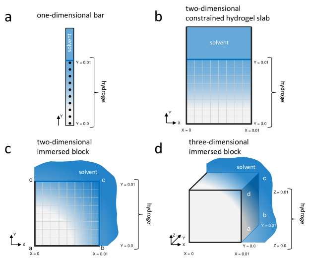
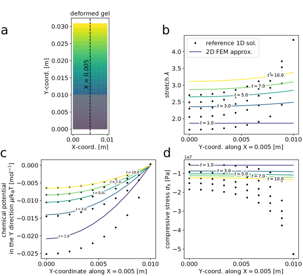
Four representative prototype problems are introduced. First, we consider a one-dimensional transient swelling of a hydrogel bar along the -direction. The bar is fixed at and free at where . At this latter end, the bar is exposed to a non-reactive solvent (see Figure 1a). The deformation gradient takes the form
| (69) |
occurring along the direction. For perfectly incompressible models (i.e., constitutive models I and II), it then results in , that is the total stretch is equal to the swelling volume change and inversely proportional to polymer volume fraction. Furthermore, from the equilibrium condition (10), it follows that , which, after considering traction free boundary conditions, leads to and, in consequence, . This problem has been studied previously by both linear and nonlinear theories, e.g., [6, 7]. Due to the simplicity of its numerical settings, this case study will serve as a reference, providing an estimate of the correct order of magnitude of the quantities of interest, i.e., , , or , in more complex case studies.
As a second example, we investigate the transient swelling of a constrained hydrogel slab in a two-dimensional setting in-plane strain (in the plane). In this example, the hydrogel block is placed in a rigid container with frictionless walls, and the deformation in the direction is constrained. Only the upper part of the hydrogel is exposed to a non-reactive solvent (see Figure 1b). This example has been previously considered by, e.g., [12] and [34], and represents the 2D counterpart of the previously introduced 1D example. However, it is noteworthy that the one-dimensional problem is numerically solved for a single scalar field (representing either or depending on the constitutive model), and the other quantities of interest are computed in the post-processing stage. On the other hand, the numerical solution of the two-dimensional problem is obtained by considering the complete sets of unknowns, that is, a scalar field describing the fluid content and the vector displacement field . Then, quantities of interest (e.g., the chemical potential ) are computed in the post-processing stage.
As a third example, we consider the transient free-swelling in a two-dimensional setting (in the plane) of a polymer gel with an initially square cross-section. A free hydrogel block is immersed in a non-reactive solvent. Due to the symmetry of the deformation, only a quarter of the whole model needs to be considered (see Figure 1c). A similar setup to this example can be found in, e,g., [13] and [34]. At the steady state, the deformation gradient is uniform within the domain, reading in the Cartesian representation as:
| (70) |
with referring to the (constant) 2D final stretch at the steady state.
The fourth and last example corresponds to the extension of the two-dimensional block example into three-dimensions, namely, a cube is immersed in a non-reactive solvent to swell due to the solvent absorption freely (see Figure 1d). In the steady state, the deformation gradient results:
| (71) |
with referring to the (constant) 3D final stretch at the steady state. This simulation resembles that presented, e.g., by [38] and will be only performed considering the constitutive model I.
We estimate the convergence order with a well-known heuristic formula. Let us denote the errors by , , and , where is the mesh size parameter as before. Under the assumption that our discretized problem has a convergence order of , then each error should be roughly times the previous error. Therefore, we can estimate by taking the logarithm base of the error ratios as:
| (72) |
5.1 Constitutive model I
One-dimensional transient swelling. Here, we follow the ideas presented by [34]. Recalling equations (34) and (35) with equation (69), the balance of linear momentum (10) reduces to:
| (73) |
Additionally, the fluid balance equation (11) in a one-dimensional setting yields
| (74) |
Differentiating equation (73) with respect to yields
| (75) |
Substituting equation (75) into equation (74) leads to a nonlinear partial differential equation with respect to .
The weak discretized form of equation (74) reads
| (76) |
where is given by equation (75) evaluated at . After solving equation (76), the chemical potential can be obtained from (73) and the stress component in the direction orthogonal to swelling as , with from equation (35).
The numerical results after solving equation (76) with the FEM are presented in Figure 2 (black dots). A one-dimensional mesh is created to discretize the hydrogel bar, with the number of elements and time steps defined from a convergence study on (results not shown). In the end, the reference solution is obtained with elements and time steps. The boundary condition at is obtained after solving equation (73) for with , which yields . The initial condition is defined as . It is worth mentioning that the obtained results accurately capture the ones presented by [34] in Figure 3 therein for the same problem setup.
Two-dimensional constrained hydrogel slab. Constitutive model I is now solved for the constrained hydrogel slab considered in Figure 1b.
Figure 2 presents the comparison between the solution previously obtained for the one-dimensional bar (black dots) and the two-dimensional constrained slab examples (different colored lines). For the two-dimensional case, we show results from different simulations with increasing number of elements and time steps. The deformed hydrogel at is displayed in Figure 2a, and a time step equal to ( time steps) was used to get Figure 2a. It is observed from Figures 2b - d that differences in numerical solution are rather small for mesh densities higher than . A zoom-in is included in Figure 2b to better distinguish between the different mesh densities. The discrepancy between the one- and two-dimensional cases can be assessed from Figure 2, which shows the effect of approximating the time derivative in the fluid concentration balance through the displacement and increasing the problem’s dimension.
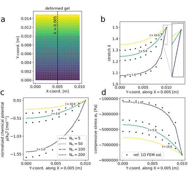
From Figure 2c, it is observed that the chemical potential’s rate increases fast in the beginning when the solvent starts entering the gel and becomes slower when it tends to the steady state. Stress follows a similar pattern as observed in Figure 2d. This behavior can be understood as follows. The gradient of is relatively large close to the top surface, at , and the compressive stress in the interior part of the hydrogel is the smallest, which are both helpful for the diffusion of the solvent content. The hydrogel’s network is relaxed and allows easy solvent absorption. The gradient of becomes smaller and larger as the solvent’s concentration increases in the hydrogel. This prevents the solvent from penetrating the hydrogel further and slows the diffusion process. There is less space within the hydrogel network, and it starts to saturate. Therefore, each quantity approaches the corresponding steady solution at a decreasing rate.
Next, a computational convergence analysis is performed to investigate the robustness and computational cost of the monolithic approach. We focus on investigating the effect of mesh density and the time step size on the behavior of the implemented numerical algorithm. We aim to understand how these parameters influence the performance of the algorithm in solving the nonlinear system of equations associated with the FEM discretization.
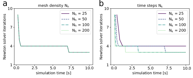
First, we conduct performance studies of the Newton solver for each time step to assess its efficiency in solving the nonlinear equations. We observe whether the mesh density and time step size influence the number of Newton iterations, determining if it remains consistent throughout the simulation. Figure 3 depicts time versus the number of Newton iterations, where Figure 3a showcases variations in mesh density and Figure 3b displays variations in time step size. From these findings, it is clear that at the beginning of the simulation, the number of Newton iterations is highest but subsequently decreases until it reaches a steady value of three iterations.
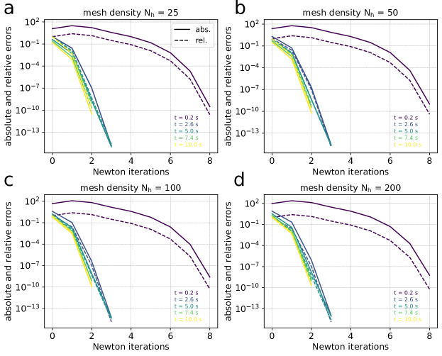
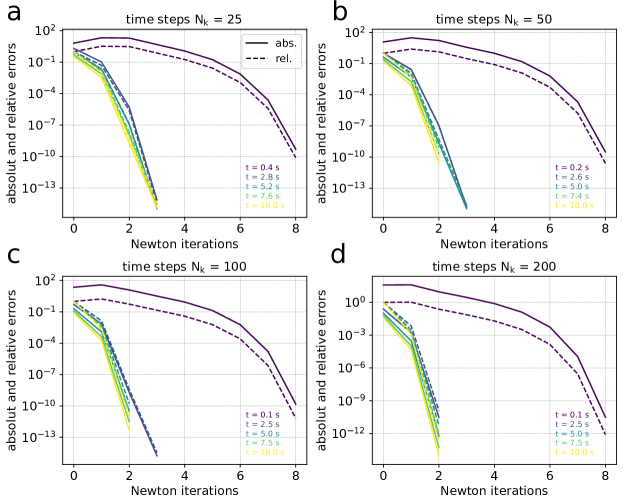
Additionally, we examine the Newton algorithm’s convergence behavior at five different time points during the simulation. We aim to confirm whether the Newton iteration has quadratic convergence in error. We also investigate whether changes in mesh density or time steps impact the Newton iteration’s convergence. Figures 4 and 5 demonstrate the convergence behavior, considering both absolute and relative errors. Figure 4 presents the results for various mesh density values, while Figure 5 displays the results for different time step sizes. Figures 4 and 5 reveal that the error decays very quickly for all the cases, except for the first iteration. But, the Newton iteration also converges in only iterations in this case. These results support the efficiency and robustness of the Newton algorithm. These findings are relevant as they assure the reliability of the numerical solution for the coupled problem solved using a monolithic approach.
After establishing that the Newton solver is reliable, we test whether using Taylor-Hood elements and the Euler method leads to the expected convergence in space and time. Specifically, we measure the error for various mesh densities and time step sizes with respect to the highest fidelity solution and the values of both displacement and chemical potential at the center of the top face of the two-dimensional hydrogel slab.
The convergence analysis is detailed in Tables 2 and 3, where the results demonstrate a second-order convergence for spatial discretization and a first-order convergence for temporal discretization. These findings are in accordance with the theoretically predicted orders from the FEM and Euler discretization scheme.
| Level |
|
|
Elements | DoFs | (0.5.1.0) | L2 error for | (1.0.1.0) | L2 error for | |||||
| 1 | 25 | 50 | 0.04 | 1250 | 5878 | -0.44017195 | 1.3896e-4 | 0.33459041 | 3.5884e-5 | ||||
| 2 | 50 | 50 | 0.02 | 5000 | 23003 | -0.43999694 | 3.4425e-5 | 0.33461516 | 9.0131e-6 | ||||
| 3 | 100 | 50 | 0.01 | 20000 | 91003 | -0.43994541 | 7.1092e-6 | 0.33462156 | 1.9465e-6 | ||||
| 4 | 200 | 50 | 0.005 | 80000 | 362003 | -0.43993062 | – | 0.33462318 | – | ||||
| conv. order | 1.80 | 1.93 | 1.98 | 1.93 |
| Level |
|
|
(0.5.1.0) | L2 error for | (1.0.1.0) | L2 error for | |||||
| 1 | 25 | 25 | 0.4 | -0.44915384 | 1.2353e-2 | 0.33195688 | 3.1447e-3 | ||||
| 2 | 25 | 50 | 0.2 | -0.44017195 | 5.5713e-3 | 0.33459041 | 1.4267e-3 | ||||
| 3 | 25 | 100 | 0.1 | -0.43534375 | 1.9333e-3 | 0.33601343 | 4.9668e-4 | ||||
| 4 | 25 | 200 | 0.05 | -0.43277477 | – | 0.33677258 | – | ||||
| conv. order | 0.91 | 0.90 | 0.91 | 0.88 |
Finally, it is noteworthy that we tested both monolithic and partitioned approaches for the solution of the constitutive model I by [34]. However, only the monolithic implementation produced physically consistent results. The reason seems to be due to the reformulation of the concentration-time derivative. The time-dependent concentration term is expressed in terms of in equation (25). Hence, such a term is highly nonlinear in terms of displacements, and its accuracy is highly affected by the adopted spatial discretization. Moreover, if the deformation process is very slow, i.e., , which is the case here, the time-dependent term in the balance of fluid concentration may become negligible, and this equation becomes quasi-static. These issues cause some numerical difficulties in the staggered approach to capture the transient behavior of the coupled problem.
Two-dimensional free swelling of a square block. A square block is immersed in a solvent with a reference chemical potential , as illustrated in Figure 1c. Recalling equations (34) and (35), and following the same procedure as in [34], the theoretical value of the steady state stretching results (see equation (70)).
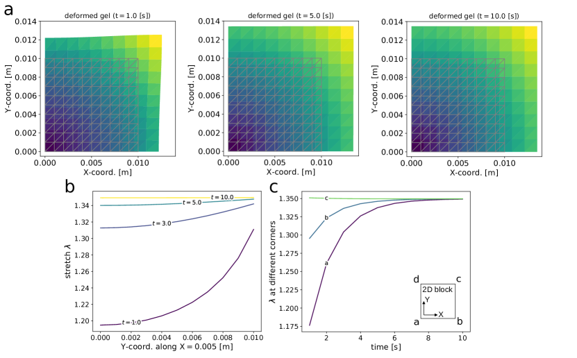
Figure 6 displays the simulation results of the transient diffusion-deformation process for the two-dimensional square block. The thick gray line in each subfigure in Figure 6a indicates the reference body. From Figure 6a, it is evidenced that the initially square block gets distorted at the beginning of the deformation process while swelling. The origin is the pronounced gradient in the early stage of the transient behavior as evidenced in Figure 6b. This distortion vanishes as time progresses and all corners reach a similar stretching value as Figure 6c shows. The two-dimensional blocks exhibit a diffusion-deformation process that aligns with the one observed in the two-dimensional slab. The final stretch reaches the steady state at the previously computed theoretical value .
Three-dimensional free swelling cubic block. The last example corresponds to the extension of the previous example from two to three dimensions as illustrated in Figure 1d. The steady-state stretching is estimated to be , which can be used to verify the simulation results at the steady state.
Figure 7 presents the simulation results of the transient diffusion-deformation process for the three-dimensional block. Compared to the two-dimensional block, the cube is less distorted, as seen in the and plane projections in Figure 7a. This can be explained by the increment in the diffusivity coefficient from to , where the latter is the minimum value that leads to the Newton algorithm iteration convergence. The diffusivity effect is observed in Figure 7b when compared to Figure 6b. The former displays a faster evolution of the stretch over time. Figure 7c shows the stretch evolution at different corners. It is observed that each observed corner presents a different stretch at the beginning of the simulation, but it fades over time. Consequently, as illustrated in Figure 7a, the three-dimensional block recovers its cube shape.
It is noted that the two-dimensional and three-dimensional problems are addressed without altering the diffusion-deformation model or its constitutive equations. Nonetheless, adjusting the diffusivity coefficient value was necessary. This is because a pronounced stretch gradient results in high-stress values and excessive distortion of the elements used for domain discretization as more degrees of freedom are added to the problem. This stability issue is commonly encountered in diffusion-deformation studies of hydrogels with non-reactive solvent absorption (refer to [7] for an in-depth discussion). Although beyond the scope of this study, stabilization methods can be employed to overcome this issue (see [29, 4] for more information). Our results provide a foundation for testing some of the approaches.
5.2 Constitutive model II
The second model under consideration is composed of the balance equations (10) and (11) together with constitutive equations (37) and (38).
One-dimensional transient swelling. Here, we follow the ideas presented by [12]. By considering the 1D deformation gradient in equation (69) under the incompressibility condition, the stress equation (37) yields:
| (77) |
Hence, it results:
| (78) |
Notice that this expression for is case specific and equation (78) holds true exactly only in the present 1D case. After some manipulations, the balance of fluid concentration given in equation (48) can be rewritten as
| (79) |
with
| (80) |
obtained after differentiating equation (38) with respect to .
The discretized weak form of equation (79) reads
| (81) |
where is given by equation (80) evaluated at . Again, equation (81) can be directly implemented in FEniCs with the corresponding boundary and initial conditions and solved using the FEM. Solution of equation (81) serves as a reference solution for the diffusion-deformation problem adopting constitutive model II. The stress can be computed replacing into equation (37), yielding:
| (82) |
which for results in a compressive stress state. Whereas the chemical potential in equation (38) becomes
| (83) |
after the definition of .
The numerical solution of equation (81) is presented in Figure 8 (black dots). A one-dimensional mesh is created to discretize the hydrogel bar. As a result of a convergence study, the final number of elements equals , and time steps are chosen (). The boundary condition at is determined from equation (38), which gives . The initial condition is defined as , which corresponds to a pre-swollen state conveniently chosen to alleviate the numerics and allow for a comparison between the one and two-dimensional models. In the original work by [12], this one-dimensional problem is numerically approximated using a finite difference method in space. The simulation results here obtained with the FEM can be quantitatively compared to those reported by [12] for a similar example (see Figures 3, 5, and 7 in [12]).
Two-dimensional constrained hydrogel slab. Constitutive model II is solved for the constrained hydrogel slab considered in Figure 1b. Initial and boundary conditions for are kept analogous to the one-dimensional case. Hence, since we have a dominant diffusion along the -direction also in this case and an analogous stress state, we approximate the Lagrange multiplier by employing the one obtained in the 1D case, i.e. with equation (78). Under the limitations of such approximation, the stress for the two-dimensional case hence reads:
| (84) |
after replacing equation (78) into equation (37). Since the same approximation for would be inaccurate in a free swelling condition, we will not face these case studies for constitutive model II.
Figure 8 presents the comparison between the one-dimensional bar (black dots) and two-dimensional constrained slab examples (different colored lines). The one-dimensional simulation is taken as the reference solution to the problem. The two-dimensional slab problem is solved for different mesh densities and different number of time steps. It was concluded that a mesh density of and time steps are enough to produce accurate results, so the following simulation results are produced using this simulation setup. The deformed hydrogel at is displayed in Figure 8a. Figures 8b - d show the time evolution of , and . It is observed that the numerical solutions for the one and two-dimensional problems coincide. This is not surprising since the large deformation displayed by the hydrogel slab makes it behave like a one-dimensional bar.
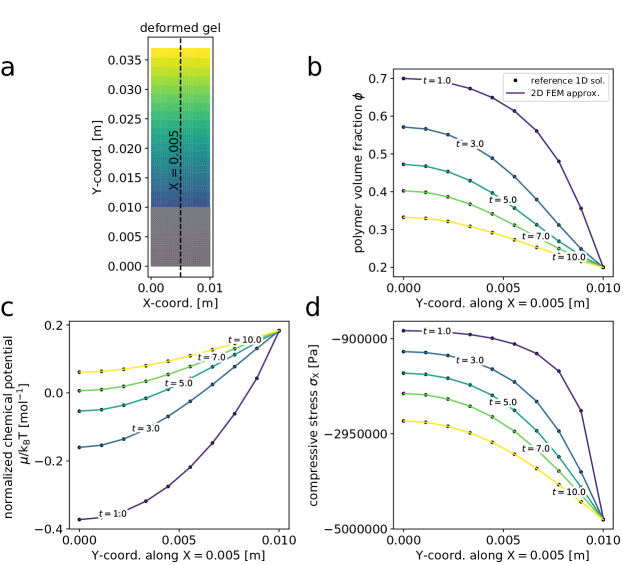
In Figure 8c, it is observed that the chemical potential’s rate increases fast in the beginning when the solvent starts entering the gel and becomes slower when it tends to the steady state. The pronounced gradient of along the spatial dimension in the beginning and a relaxed polymer network facilitates solvent absorption. As the gradient of flattens out and the compressive stress increases, solvent diffusion slows down.
[6] and [14] proposed to solve an additional nonlinear equation either for or at the Gauss integration point to fully determine the time derivative term and then solve the balance of fluid concentration for the chemical potential. If equations (43) and (48) are solved for , either equation (42), (38), or (46) must be solved as an implicit nonlinear equation at each Gauss integration point for either or , depending of the adopted constitutive model, as suggested by [7] and [12, 14].
In [14], the coupled problem was solved using the commercial software Abaqus, via an UMAT routine. The coupled problem was solved for , , and . In particular, was defined as a local variable, and the nonlinear equation (38) was solved at each Gauss integration point. This approach allowed to fully determine the time derivative in equation (48)2 at each time instance. Thus, a static problem for and is solved also at each time step. A similar idea was adopted by [7].
We decided to test an alternative approach. That is, to find a suitable expression for in equation (48) from the constitutive equation (38). Then, solve the couple problem only for and . Such an approach allows us to avoid the computation of at each integration point. By following this approach, we noticed that the solution becomes less prompt to numerical instabilities, and monolithic and staggered formulations can be adopted to solve the resulting coupled problem. It is worth remarking that without the automatic differentiation capabilities of FEniCs, the computation of can be a very tedious task, and it is not difficult to imagine that was the reason why [14] opted for their approach.
We conduct an investigation to assess the staggered approach’s behavior. We verify the number of staggered iterations between the displacement and polymer volume fraction sub-systems and, as for the monolithic case, we examine the effects of mesh density and time step size on the algorithm’s performance, focusing particularly on the Newton solver’s efficiency and convergence.
For the staggered solution, we modify the strategy slightly. Instead of computing the total number of Newton iterations required for convergence, we compute the average number of Newton iterations over the inner iteration loop for each time increment for the displacement and polymer volume fraction sub-systems. This approach provides us with insights into the staggered solution’s convergence behavior and whether the number of staggered and Newton iterations remains stable throughout the simulation time. It allows us to gauge the efficiency and stability of the staggered approach, and compare it to the monolithic approach.
Figure 9 illustrates the time versus the staggered and Newton iterations for different mesh densities and time step sizes. Figures 9a and 9d show how many staggered iterations are necessary at each time step to reach an error lower than both for and , respectively. It is observed that the number of iterations is never higher than three, independent of the mesh density and time step size. This highlights the effectiveness of the staggered approach.
The convergence patterns for the Newton iterations and the impact of variations in mesh density and time step size were consistent with those observed in the monolithic approach. Figures 9b, e focuses on the Newton iteration for the displacement sub-system, whereas Figure 9c,f reports the Newton iterations along time for the polymer volume fraction sub-system, for different mesh densities and time step sizes, respectively. Results in Figure 9 reveal a similar trend to the monolithic case regarding the Newton iterations at each time increment.
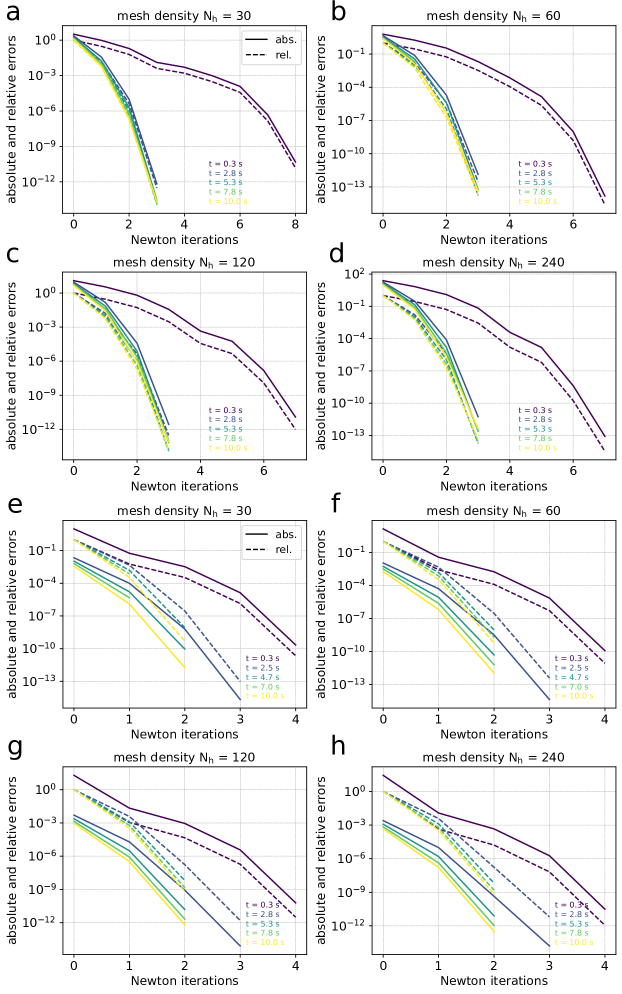
Additionally, we explored the Newton algorithm’s convergence behavior at five distinct simulation moments, examining the quadratic convergence in error and the influence of mesh density and time step size. Figure 10 shows the error decay with respect to the Newton iterations. Sub-figures 10a, b, c, d correspond to the displacement, while sub-figures 10e, f, g, h refer to the polymer volume fraction, both for different mesh densities. The results are analogous to the monolithic approach, where the absolute and relative errors decay fast as the Newton iteration increases, demonstrating the staggered approach’s robustness.
The observed similarities in the convergence behaviors between the monolithic and staggered approaches further underline the robustness and reliability of the numerical solutions, confirming the applicability of both methods to the coupled problem at hand.
Concerning convergence analyses for the discretization itself, for the Taylor-Hood elements and Euler method, our findings for spatial and temporal discretization yielded a second-order and first-order convergence, respectively. These outcomes are summarized in Tables 4 and 5, reinforcing the staggered approach’s validity in solving the coupled diffusion-deformation problem.
| Level |
|
|
Elements | DoFs | (0.5.1.0) | L2 error for | (1.0.1.0) | L2 error for | |||||
| 1 | 30 | 40 | 0.033 | 1800 | 8403 | 0.31318141 | 2.2590e-5 | 2.83246074 | 1.4800e-4 | ||||
| 2 | 60 | 40 | 0.016 | 7200 | 33003 | 0.31309735 | 5.4560e-6 | 2.83288465 | 3.4709e-5 | ||||
| 3 | 120 | 40 | 0.008 | 28800 | 130803 | 0.31307316 | 1.2288e-6 | 2.83299197 | 9.0328e-6 | ||||
| 4 | 240 | 40 | 0.004 | 115200 | 520803 | 0.31306639 | – | 2.83301882 | – | ||||
| conv. order | 1.83 | 2.02 | 2.00 | 2.14 |
| Level |
|
|
(0.5.1.0) | L2 error for | (1.0.1.0) | L2 error for | |||||
| 1 | 30 | 20 | 0.5 | 0.31996593 | 8.2017e-3 | 2.72595105 | 9.6975e-02 | ||||
| 2 | 30 | 40 | 0.25 | 0.31309911 | 3.7086e-3 | 2.80367321 | 4.3200e-02 | ||||
| 3 | 30 | 80 | 0.125 | 0.30939811 | 1.2936e-3 | 2.84445820 | 1.4871e-02 | ||||
| 4 | 30 | 160 | 0.0625 | 0.30741375 | – | 2.86582984 | – | ||||
| conv. order | 0.90 | 0.90 | 0.93 | 0.92 |
5.3 Constitutive model III
The third model under consideration comprises the balance equations (10) and (11) together with constitutive equations (40) and (42).
One-dimensional transient swelling. The basic ingredients to describe the hydrogel deformation considering an energetic constraint were presented by [6, 7]. By considering the 1D deformation gradient in equation (69), the balance of fluid concentration reads
| (85) |
with
| (86) |
and
| (87) |
where refers to the initial swelling ratio of the gel.
The discretized weak form of equation (85) reads
| (88) |
where and are given by equations (86) and (87) evaluated at , respectively. Equation (88) can be solved using the FEM with FEniCS. The postprocessing quantities and results:
| (89) |
and
| (90) |
respectively. Notice that in equation (42) was replaced in by to get equation (89). More details about the derivation of equations (89) and (90) can be found in appendix A of [7].
Two-dimensional constrained hydrogel slab. Example’s geometry corresponds to that illustrated in Figure 1b. Initial and boundary conditions correspond to those defined for the one-dimensional case.
Figure 11 presents the comparison between the one-dimensional bar (black dots) and two-dimensional constrained slab examples (different colored lines). The two-dimensional slab problem is solved for a mesh density and time steps (). This setup yields an acceptable numerical accuracy for the two-dimensional configuration. The deformed hydrogel at is displayed in Figure 11a. Figures 11b - d show the time evolution of , and . It is observed that the numerical solutions for the one and two-dimensional problems are on the same order of magnitude and get closer as the two-dimensional slab becomes larger and progressively resembles a one-dimensional domain. The same pattern was observed for the constitutive model I. However, the hydrogel experiences a lower level of stretch when considering the two-dimensional setup. This is the effect of determining first through the nonlinear equation and then from the static PDE. The boundary condition can only be imposed on , not as in the one-dimensional case.
The transient behavior of the hydrogel follows the already observed evolution for constitutive models I and II. At the beginning of the deformation, the solvent enters the gel faster because of the high gradient and low compressible stress. From Figure 11, it is noticed that the hydrogel slab undergoes a rather large deformation, i.e., the final size is about times the original one, despite the presence of the energetic constrain in the free energy function. The small shear modulus value can justify this large deformation.
Constitutive model III as considered in this work was formally presented by [6] and solved using the FEM by [7]. The coupled problem was solved for , , and . In particular, was defined as a local variable, and the nonlinear equation (42) was solved at each Gauss integration point to determine the time derivative in equation (43) at each time instant. Next, and are computed by the solution of a static problem defined by equations (10) and (11) at each time step.
Here we tried to find a suitable expression for in equation (48) from the constitutive equation (42) using FEniCS automatic differentiation tools and avoid the solution of the nonlinear equation at the Gauss points for the two-dimensional example. Although we got some numerical results, these appear highly inaccurate compared to the reference 1D outcomes. Consequently, we only report the results obtained following [7] original formulation.
It should be highlighted that among the constitutive models accounted for in this work, constitutive model III numerical solution is the most fragile. There is not much room to explore different values for the model parameters. Small changes in their values would lead to the divergence of the Newton-Raphson algorithm. It is also not possible to arbitrarily increase the mesh density or make the time step smaller. This is not surprising since [7] presented a detailed analysis of the induced instabilities in hydrogels in the presence of geometrical constraints. These instabilities arise because the exposure of a gel to a fluid not only leads to a large increase in volume but also to a wave-like buckling pattern. Free surfaces expand due to the species influx and are bonded to unswollen inner parts of the gel simultaneously. For high osmotic pressure, this mechanism leads to buckling patterns, that have extensively been analyzed within experimental setups (see, e.g., [22, 16, 31] for more details on hydrogels instabilities).
Due to this numerical fragility, it was not possible to perform a convergence analysis in the same manner as for the two previous constitutive models. However, for the chosen simulation setup presented in this sub-section, both the absolute and relative errors decay faster as the Newton iterations increase, in a manner similar to that observed for constitutive model II (see Figures 4 and 5).
Two-dimensional free swelling of a square block. Figure 1c illustrates the considered example. For the solvent concentration boundary conditions, the edges ab and ad (the symmetry edges) are prescribed a zero fluid flux, and on the edges bc and cd, the chemical potential is set equal to zero. The initial condition for is defined as . In this case, it was not necessary to apply a time-ramping strategy.
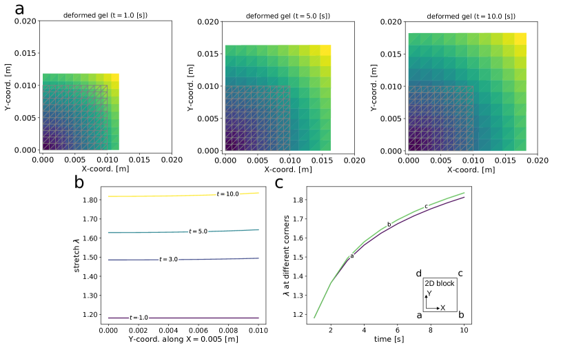
The simulation results for the two-dimensional square block are presented in Figure 12. The box plotted with a thick gray line in Figure 12a corresponds to the reference body before undergoing deformation. In contrast to the constitutive model I, the block tends to keep its square shape along the simulation time. This can be attributed to the value of the diffusivity that prevents high gradients as observed in Figure 12b. However, we chose this simulation setup because it leads to numerical convergence. For simulation setup producing more pronounced gradients, bigger distortion, or larger deformations, suitable stabilization techniques are required (see, e.g., [29, 4] for some approaches), which are out of the scope of the current research. An important difference between constitutive model III and the previous constitutive models is that does not tend to a steady state value as time simulation progresses. This can be appreciated from Figure 12c.
5.4 Constitutive models IV and V
The fourth and fifth models under consideration are composed of the balance equations (10) and (11) together with constitutive equations (45) and (46) for the stress and chemical potential, respectively.
To avoid redundancies, we only present results for the two-dimensional free swelling of a square block with constitutive models IV and V. It is worth recalling that the main difference between constitutive model II and IV - V is the addition of an energetic component in the free energy function, thus eliminating the need to introduce a Lagrange multiplier as in constitutive model II.
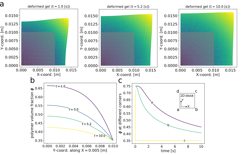
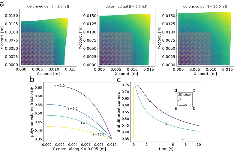
6 A reference benchmark problem
In this section, the two-dimensional square block problem is studied again as a unified benchmark problem for the diffusion-deformation of hydrogels. As a matter of fact, previous results cannot be directly compared due to the disparate value of the material parameters selected by authors in the original papers (and adopted for the prototype problems presented in the previous section). Our goal here is to have a unique reference simulation example and show the differences in the response for each constitutive equation. We are interested in testing how much the diffusion-deformation behavior is affected by the different constitutive choices under the same simulation setup.
Hydrogels are a type of material that can vary significantly in their physical properties due to factors such as the particular polymer used, the degree of crosslinking, and the presence of any additives [9]. As such, the shear modulus () and bulk modulus () can have a wide range of values. Typically, the shear modulus of hydrogels can range from to , with softer, more water-rich gels being at the lower end of the scale and more crosslinked or polymer-rich gels being at the higher end. Among the studies considered in this research, we found very different values for the shear modulus ranging from in [12, 13] to as reported by [35].
Similarly, the bulk modulus, which is a measure of a material’s resistance to uniform compression, can also vary widely for hydrogels. The bulk modulus is typically larger than the shear modulus. For many hydrogels, the bulk modulus can range from around to several . However, these values should only be used as a rough guide, as the specific values for any particular hydrogel can vary significantly depending on its formulation and preparation details. One needs to refer to specific experimental data for the particular hydrogel of interest for a precise value. The most common value for reported in the reviewed papers was .
In the present study, motivated by state-of-the-art values, we choose and . The diffusion coefficient is used as the free parameter to tune the simulation such that the results become comparable and the numerical stability is guaranteed. All other parameters remain the same as for the previously reported simulation results. Notice that this simulation setup is similar to the one used to solve constitutive models II, and IV - V and it was inspired by [14].
H
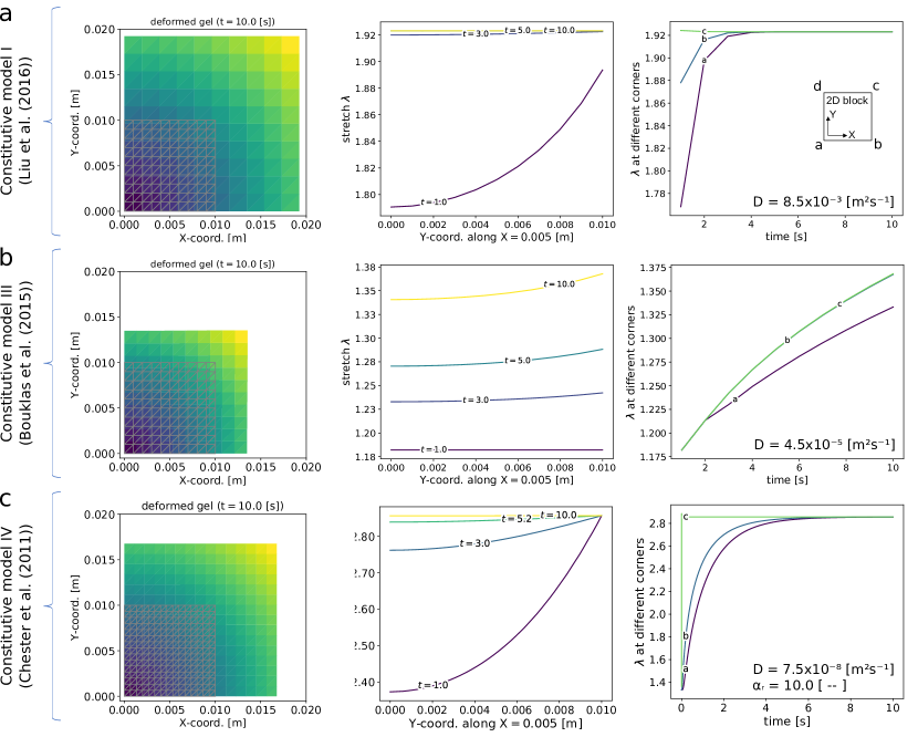
Figure 15 shows the simulation results for the two-dimensional square block problem. Results are reported for constitutive models I, III, and IV. The reason for this selection is twofold: i. constitutive model II introduces an additional field represented by the Lagrange multiplier, thus requiring ad hoc numerical treatments outside of the scopes of present work; ii. the same example was solved for constitutive model V with the same parameters and results in Figure 15 can be directly compared with those plotted in Figure 14.
From Figure 15, first column, it is possible to observe that the level of deformation achieved in each case by the end of the simulation is different despite the similarity of the parameters. However, it is not on the deformation or stretch where the main difference between the different models becomes evident. It is on the transient evolution of the solvent as appreciated in the second and third columns of the figure. Constitutive models I and IV reach their steady state in about (Figure 15a, third column) and (Figure 15c, third column), respectively, whereas constitutive model III is far from reaching the steady state (Figure 15b, third column).
It is important to note that the diffusivity values used in the benchmark problem for constitutive models I and III are the lowest possible before encountering numerical issues. For constitutive models III - IV, it is feasible to set the diffusivity to , matching constitutive model I. However, given our simulation setup, this is an exceptionally high value. Consequently, the system will reach steady in both scenarios almost immediately, eliminating any transient behavior. In summary, the mentioned diffusivity values differ significantly from each other. They belong to different time scales. This difference can be attributed to the distinct solution strategies adopted for solving the diffusion equation in each case. We delved into the specifics of this when introducing each constitutive model.
One takeaway drawn from this comparison study is that further refinement may be required for the constitutive models such that closer predictions are achieved. In particular, each model predicts a different level of deformation and requires a fine-tuning of some parameters to ensure numerical convergence. This can complicate the model’s experimental validation because it could lead to different values of the material parameters and, for instance, ambiguity regarding which values are correct and their interpretability. Nonetheless, there is still room for improvement in selecting the energetic component of the constitutive model, which can fix the issue. In the end, all constitutive models capture the diffusion-deformation process in a reasonable way and offer valuable insights into the coupled problem.
7 Conclusion
This study presented a detailed classification and analysis of various nonlinear models that depict the diffusion-deformation process in hydrogels caused by non-reactive solvent absorption. We have consolidated these theories into a unified framework, demonstrating that, despite not being evident, all theories follow equivalent thermodynamic arguments. For instance, while having a common set of governing equations, each model showcases differences in the enforcement of incompressibility and formulation of the constitutive model — particularly in terms of the free energy function’s components, mainly at the energetic level. At present, further research appears necessary to conveniently account for the energetic component, ultimately aiming for a cohesive and unified constitutive model.
Different numerical approaches adopted by various researchers to solve these models were analyzed. Our implemented numerical methods presented reasonable predictions for the diffusion-deformation process. However, our findings suggest that the superiority of one strategy over another remains inconclusive. The selection of an appropriate model should be grounded in a comprehensive understanding of the hydrogel’s composition and must be validated experimentally. Notice that some of the theories here introduced have been extended to account for temperature variations, chemical reactions, and damage (refer to, e.g., [42, 39, 28, 24] for more details). So, they represent a solid foundation for the study of elastomeric materials.
We emphasized on discerning the differences among the leading models in the literature and verifying whether the results presented by different authors are still valid in light of open-source general-purpose software available nowadays, such as FEniCS. To this end, an important part of this work is Section 3 with the mathematical classification and resulting numerical discretization and algorithms. These allowed us to carefully design mathematical formulations, which were then implemented and used to study the previously mentioned models.
Advances in automated solution techniques for the finite element method (FEM), such as FEniCS, provide the user with a streamlined approach for solving systems of partial differential equations compared to traditional model development. Unlike models implemented on commercial software (e.g., Abaqus), the implementation of our models grants users considerable control over several components.
The simulation results indicate that there is not a one-size-fits-all model compatible with the parameters across all scenarios. Depending on the specific problem configuration being simulated, adjustments to one or multiple parameters are necessary to guarantee the numerical stability of the solution. Our observations in Section 5 revealed a strong dependency of the numerical solution’s convergence on the diffusion coefficient and bulk modulus value. In fact, very different diffusion coefficients for each example featured in this study were required. Nonetheless, once a suitable value for the material parameters is identified, the numerical solution achieves reliable accuracy and robustness, as evidenced by the convergence analysis. Here, a consistent number of Newton iterations was displayed along the simulation time to reach absolute and relative errors smaller than . Moreover, concerning the spatial and temporal discretization, quadratic and linear convergence orders, respectively, for the FEM and Euler schemes for both the monolithic and staggered approaches were observed.
Furthermore, constitutive model III stands to be the more fragile in terms of numerical stability. Because constitutive model III directly penalizes the material compressibility, it calls for a numerical solution using a mixed formulation where the stress becomes a primary variable as it is standard in the literature dealing with incompressible materials (see, e.g., [8] or [40]).
Another observation was regarding the application of boundary conditions. Depending on the specific simulation scenario, it might be necessary to adopt a time-ramping strategy to prevent numerical instabilities, which is well known in continuum mechanics and due to the mathematical functional framework in order to have compatible conditions. However, these mathematical assumptions might not be met in many engineering applications. Therefore, one must be careful with any assumption made while numerically solving the problem at hand to avoid unphysical numerical results.
As an overall outcome, in Section 5, we found that each model presents diverse deformation states and solute concentrations within the hydrogel, highlighting the complexity of the investigated problem. It is evident that pinpointing a single appropriate model to describe the diffusion-deformation of hydrogels remains a challenge, given the different calibration mechanisms each offers. These differences underscore the need for more comprehensive experimental data to reconcile these theoretical distinctions with actual observations. With the models’ validation, we can transition from merely describing the process to predicting hydrogel behavior, thereby using the model for designing new materials or optimizing the mechanical properties of existing ones.
Some efforts have been made to validate the diffusion-deformation process of hydrogels as predicted by the coupled model. For example, [11] performed a validation of a very similar theory as presented by [6] with a major focus on the linear theory. Several measurements of the strain experienced by a gelatin-glycerol-water hydrogel under free-swelling conditions are reported, and the best-fitting parameters are identified. Neither the time evolution of the diffusion process nor the internal stress were investigated. [5, 1] performed an experimental work to validate an extension of the original models presented by [14]. The extended models account for the viscoelastic response of elastomeric gels under isothermal and non-isothermal conditions. Again, the transient behavior of the diffusion process is neglected, and only the stresses are computed for the steady state under external loading conditions. Consequently, no study has been carried out to validate the models as presented in this study.
Supplementary information No supplementary information was produced from this research.
Acknowledgments MM acknowledges the funding of Regione Lazio (project n. A0375-2020-36756, Progetti di Gruppi di Ricerca 2020, POR FESR LAZIO 2014) and the Italian National Group for Mathematical Physics GNFM-INdAM.
Declarations
Funding: The authors declare that no funds, grants, or other support were received during the preparation of this manuscript.
Conflict of interest/Competing interests: On behalf of all authors, the corresponding author states that there is no conflict of interest.
Code availability: Codes to reproduce the results presented in this manuscript can be freely accessed at the following link: https://doi.org/10.25835/5v49yfk0.
Appendix A Alternative forms: the notion of active chemical potential
The total deformation gradient depends on fluid concentration from equation (8). To better distnguish between elasti- and fluid-related effects, the stress power can be reformulated as:
| (91) |
where represents the PK1 stress tensor from the intermediate to the current configuration (also referred to as the elastic PK1) and is the Mandel stress tensor in the intermediate configuration555In the state-of-the-art, two different stress measures can be found in the present context, namely and , [12]. These definitions are analogous but the corresponding stress measures refer to the reference configuration.:
| (92) |
At this standpoint, a mean normal pressure can be introduced,
| (93) |
representing the pull-back of the hydrostatic pressure from the current to the intermediate configuration. Finally, upon enforcing the kinematic constraint defined in equation (5), the stress-power equation (91) may be written as:
| (94) |
Hence, the local form of the second law of thermodynamics, equation (12), reads also as:
| (95) |
from which it appears convenient defining the free energy density function as function of the elastic deformation and fluid concentration , that is
| (96) |
By defining the active chemical potential as:
| (97) |
equation (95) yields:
| (98) |
from which the following constitutive choices follow for the elastic PK1 stress tensor:
| (99) |
and the active chemical potential:
| (100) |
It is straightforward to show that constitutive choices in equations (15) and (16) are equivalent to the ones in equations (99) and (100) given that:
| (101) |
In fact, by employing the chain rule and considering equation (101), it results from equation (99):
| (102) |
where it follows that by definition (cf. equation (92)), recovering the constitutive relationship for the PK1 stress tensor in equation (15).
Moreover, it results from equation(93), (97) and (100) that:
| (103) |
where, considering equation (101), the first term reads also as (accounting for the dependency from equation (8)):
| (104) |
while the second term as (with equation (102)):
| (105) |
Hence, since:
| (106) |
the chemical potential computed from equation (100) is equivalent to the one from equation (16), given that equation (101) holds true.
References
- \bibcommenthead
- Alkhoury et al [2022] Alkhoury K, Bosnjak N, Wang Y, et al (2022) Experiments and modeling of the thermo-mechanically coupled behavior of vhb. International Journal of Solids and Structures 242:111523
- Alnæs et al [2015] Alnæs M, Blechta J, Hake J, et al (2015) The FEniCS project version 1.5. Archive of Numerical Software 3(100)
- Biot and Willis [1957] Biot MA, Willis DG (1957) The elastic coefficients of the theory of consolidation. Journal of Applied Mechanics 24(4):594–601
- Böger et al [2017] Böger L, Nateghi A, Miehe C (2017) A minimization principle for deformation-diffusion processes in polymeric hydrogels: constitutive modeling and FE implementation. International Journal of Solids and Structures 121:257–274
- Bosnjak et al [2020] Bosnjak N, Nadimpalli S, Okumura D, et al (2020) Experiments and modeling of the viscoelastic behavior of polymeric gels. Journal of the Mechanics and Physics of Solids 137:103829
- Bouklas and Huang [2012] Bouklas N, Huang R (2012) Swelling kinetics of polymer gels: comparison of linear and nonlinear theories. Soft Matter 8(31):8194–8203
- Bouklas et al [2015] Bouklas N, Landis CM, Huang R (2015) A nonlinear, transient finite element method for coupled solvent diffusion and large deformation of hydrogels. Journal of the Mechanics and Physics of Solids 79:21–43
- Brink and Stein [1996] Brink U, Stein E (1996) On some mixed finite element methods for incompressible and nearly incompressible finite elasticity. Computational Mechanics 19(1):105–119
- Cascone et al [2018] Cascone S, Lamberti G, Barba A (2018) Hydrogels: experimental characterization and mathematical modelling of their mechanical and diffusive behaviour. Chemical Society Reviews 47(7):2357–2373
- Chaterji et al [2007] Chaterji S, Kwon IK, Park K (2007) Smart polymeric gels: Redefining the limits of biomedical devices. Progress in polymer science 32(8-9):1083–1122
- Chen et al [2020] Chen S, Huang R, Ravi-Chandar K (2020) Linear and nonlinear poroelastic analysis of swelling and drying behavior of gelatin-based hydrogels. International Journal of Solids and Structures 195:43–56
- Chester and Anand [2010] Chester SA, Anand L (2010) A coupled theory of fluid permeation and large deformations for elastomeric materials. Journal of the Mechanics and Physics of Solids 58(11):1879–1906
- Chester and Anand [2011] Chester SA, Anand L (2011) A thermo-mechanically coupled theory for fluid permeation in elastomeric materials: application to thermally responsive gels. Journal of the Mechanics and Physics of Solids 59(10):1978–2006
- Chester et al [2015] Chester SA, Di Leo CV, Anand L (2015) A finite element implementation of a coupled diffusion-deformation theory for elastomeric gels. International Journal of Solids and Structures 52:1–18
- Ciarlet [1987] Ciarlet PG (1987) The finite element method for elliptic problems, 2nd edn. North-Holland, Amsterdam [u.a.]
- Dervaux and Amar [2012] Dervaux J, Amar MB (2012) Mechanical instabilities of gels. Annu Rev Condens Matter Phys 3(1):311–332
- Deuflhard [2011] Deuflhard P (2011) Newton Methods for Nonlinear Problems, Springer Series in Computational Mathematics, vol 35. Springer Berlin Heidelberg
- Ehlers and Bluhm [2002] Ehlers W, Bluhm J (2002) Porous media: theory, experiments and numerical applications. Springer Science & Business Media
- Gander and Neumüller [2016] Gander MJ, Neumüller M (2016) Analysis of a new space-time parallel multigrid algorithm for parabolic problems. SIAM J Sci Comput 38(4):A2173–A2208
- Girault and Raviart [1986] Girault V, Raviart PA (1986) Finite Element method for the Navier-Stokes equations. Number 5 in Computer Series in Computational Mathematics, Springer-Verlag
- Gurtin et al [2010] Gurtin ME, Fried E, Anand L (2010) The mechanics and thermodynamics of continua. Cambridge university press
- Guvendiren et al [2010] Guvendiren M, Burdick JA, Yang S (2010) Solvent induced transition from wrinkles to creases in thin film gels with depth-wise crosslinking gradients. Soft Matter 6(22):5795–5801
- Hackbusch [1985] Hackbusch W (1985) Multi-Grid Methods and Applications. Springer
- Hajikhani et al [2021] Hajikhani A, Wriggers P, Marino M (2021) Chemo-mechanical modelling of swelling and crosslinking reaction kinetics in alginate hydrogels: A novel theory and its numerical implementation. Journal of the Mechanics and Physics of Solids 153:104476
- Hong et al [2008] Hong W, Zhao X, Zhou J, et al (2008) A theory of coupled diffusion and large deformation in polymeric gels. Journal of the Mechanics and Physics of Solids 56(5):1779–1793
- Huang et al [2020] Huang R, Zheng S, Liu Z, et al (2020) Recent advances of the constitutive models of smart materials—hydrogels and shape memory polymers. International Journal of Applied Mechanics 12(02):2050014
- Kabir et al [2018] Kabir SF, Sikdar PP, Haque B, et al (2018) Cellulose-based hydrogel materials: Chemistry, properties and their prospective applications. Progress in biomaterials 7:153–174
- Konica and Sain [2020] Konica S, Sain T (2020) A thermodynamically consistent chemo-mechanically coupled large deformation model for polymer oxidation. Journal of the Mechanics and Physics of Solids 137:103858
- Krischok and Linder [2016] Krischok A, Linder C (2016) On the enhancement of low-order mixed finite element methods for the large deformation analysis of diffusion in solids. International Journal for Numerical Methods in Engineering 106(4):278–297
- Lei et al [2021] Lei J, Li Z, Xu S, et al (2021) Recent advances of hydrogel network models for studies on mechanical behaviors. Acta Mechanica Sinica 37:367–386
- Liaw et al [2019] Liaw CY, Pereyra J, Guvendiren M (2019) Wrinkling on covalently anchored hydrogels. Wrinkled Polymer Surfaces: Strategies, Methods and Applications pp 205–227
- Lin et al [2010] Lin G, Chang S, Hao H, et al (2010) Osmotic swelling pressure response of smart hydrogels suitable for chronically implantable glucose sensors. Sensors and Actuators B: Chemical 144(1):332–336
- Liu et al [2015a] Liu Y, Zhang H, Zhang J, et al (2015a) Constitutive modeling for polymer hydrogels: A new perspective and applications to anisotropic hydrogels in free swelling. European Journal of Mechanics-A/Solids 54:171–186
- Liu et al [2016] Liu Y, Zhang H, Zhang J, et al (2016) Transient swelling of polymeric hydrogels: A new finite element solution framework. International Journal of Solids and Structures 80:246–260
- Liu et al [2010] Liu Z, Hong W, Suo Z, et al (2010) Modeling and simulation of buckling of polymeric membrane thin film gel. Computational Materials Science 49(1):S60–S64
- Liu et al [2015b] Liu Z, Toh W, Ng TY (2015b) Advances in mechanics of soft materials: A review of large deformation behavior of hydrogels. International Journal of Applied Mechanics 7(05):1530001
- Logg et al [2012] Logg A, Mardal KA, Wells G (2012) Automated solution of differential equations by the finite element method: The FEniCS book, vol 84. Springer Science & Business Media
- Lucantonio et al [2013] Lucantonio A, Nardinocchi P, Teresi L (2013) Transient analysis of swelling-induced large deformations in polymer gels. Journal of the Mechanics and Physics of Solids 61(1):205–218
- Mao and Anand [2018] Mao Y, Anand L (2018) A theory for fracture of polymeric gels. Journal of the Mechanics and Physics of Solids 115:30–53
- Pantuso and Bathe [1997] Pantuso D, Bathe KJ (1997) On the stability of mixed finite elements in large strain analysis of incompressible solids. Finite elements in analysis and design 28(2):83–104
- Saad [2003] Saad Y (2003) Iterative methods for sparse linear systems. SIAM
- Sain et al [2018] Sain T, Loeffel K, Chester S (2018) A thermo–chemo–mechanically coupled constitutive model for curing of glassy polymers. Journal of the Mechanics and Physics of Solids 116:267–289
- Sun and Tan [2013] Sun J, Tan H (2013) Alginate-based biomaterials for regenerative medicine applications. Materials 6(4):1285–1309
- Wang et al [2018] Wang X, Zhai Z, Chen Y, et al (2018) A facile, robust and versatile finite element implementation to study the time-dependent behaviors of responsive gels. Extreme Mechanics Letters 22:89–97
- Wick [2020] Wick T (2020) Multiphysics phase-field fracture: modeling, adaptive discretizations, and solvers, vol 28. Walter de Gruyter GmbH & Co KG
- Wick [2023] Wick T (2023) Space-time methods: formulations, discretization, solution, goal-oriented error control and adaptivity. https://thomaswick.org/links/Wi23_st_book_preprint_Aug_8_2023.pdf, to appear in Springer, Compact Textbooks in Mathematics
- Wloka [1987] Wloka J (1987) Partial differential equations. Cambridge University Press
- Wriggers [2008] Wriggers P (2008) Nonlinear finite element methods. Springer Science & Business Media
- Zhang et al [2009] Zhang J, Zhao X, Suo Z, et al (2009) A finite element method for transient analysis of concurrent large deformation and mass transport in gels. Journal of Applied Physics 105(9):093522