Measurements and modeling of induced flow in collective vertical migration

Abstract

Hydrodynamic interactions among swimming or flying organisms can lead to complex flows on the scale of the group. These emergent fluid dynamics are often more complex than a linear superposition of individual organism flows, especially at intermediate Reynolds numbers. This paper presents an approach to estimate the flow induced by multiple swimmer wakes in proximity using an analytical model that conserves mass and momentum in the aggregation. This analytical model was informed by and validated with empirical measurements of induced vertical migrations of brine shrimp, Artemia salina. The response of individual swimmers to ambient background flow and light intensity was evaluated. In addition, the time-resolved three-dimensional spatial configuration of the swimmers was measured using a recently developed laser scanning system. Computational experiments using the analytical model found that the induced flow at the front of the aggregation was insensitive to the presence of downstream swimmers, with the induced flow reaching an asymptote beyond a threshold aggregation length. Closer swimmer spacing led to higher induced flow, in some cases leading to model predictions of induced flow exceeding swimmer speeds required to maintain a stable spatial configuration. This result was reconciled by comparing two different models for the near-wake of each swimmer. Our results demonstrate that aggregation-scale flows result from a complex, yet predictable interplay amongst organism-scale wake structure, swimmer spacing and configuration, and aggregation size.

1 Introduction

Various species of swimming and flying organisms exhibit collective motion, characterised by coordinated movement within groups of organisms (Vicsek & Zafeiris, 2012). The emergent hydrodynamic properties of collective groups of swimming and flying organisms are vital to understanding flow-mediated communication (Mathijssen et al., 2019), fluid transport (Katija, 2012), and the hydrodynamic performance of collectives (Weihs, 1973; Zhang & Lauder, 2023). Applications of these fluid mechanics include control mechanisms for robotic swarms (Berlinger et al., 2021) and climate modelling (Stemmann & Boss, 2012).

One of the most common manifestations of collective behaviour found in the ocean is diel vertical migration (DVM). Prevalent among freshwater and marine zooplankton taxa globally, DVM involves the migration of zooplankton from deep regions in the water column during the day to shallower depths at night over a vertical distance on the order of 1 km; it is the largest migration on Earth by mass (Bandara et al., 2021). However, the scale of flow induced by a DVM event remains unresolved despite field measurements (Fernández Castro et al., 2022; Dewar et al., 2006; Farmer et al., 1987; Gregg & Horne, 2009), laboratory observations (Houghton et al., 2018), and theoretical estimates (Huntley & Zhou, 2004; Dewar et al., 2006) of biogenic mixing due to collective swimming.

Studies of flows on the individual organism scale include a comprehensive set of experimental (Lauder & Madden, 2008; Dabiri, 2005), theoretical (Derr et al., 2022; Wu, 2011) and computational (Pedley & Hill, 1999; Eldredge, 2007) estimates. Direct numerical simulation has been used to study the hydrodynamics of collective motion (Ko et al., 2023), including the mixing induced by Stokes squirmers (Ouillon et al., 2020; Wang & Ardekani, 2015; Lin et al., 2011). However, due to the nonlinear coupling between individual and collective flow fields at intermediate and high Reynolds numbers, a more general approach to connecting these individual flows to the fluid dynamics on the collective scale remains an open challenge.

At low Reynolds numbers, Stokesian dynamics (Brady & Bossis, 1988) can be used to estimate hydrodynamic interactions through linear superposition (Ishikawa et al., 2006; Pushkin et al., 2013; Lauga & Powers, 2009). For organisms characterised by high Reynolds number dynamics, the linearity of potential flow theory allows for approaches based on linear superposition to estimate the combined effect of flow within a group (Weihs, 1973, 2004). However, for swimmers operating in an intermediate Reynolds regime, such as the majority of vertically migrating swimmers in the ocean (Katija, 2012), neither Stokesian nor potential flow assumptions accurately capture the dominant hydrodynamic forces, resulting in nonlinear governing dynamical equations that are not readily suitable for linear superposition.

Although not strictly justified from first principles, superposition has been successfully applied to estimate wake interactions in wind farms without using potential flow assumptions. Initial efforts, exemplified by the linear superposition model proposed by Lissaman (1979), assumed a large wind turbine spacing and weak wake interactions to linearly sum wake velocity deficits. Subsequent critiques highlighted the potential overestimates of the wake deficit within densely arranged wind turbine arrays, where there are significant wake interactions (Crespo et al., 1999). In response to this limitation, several alternative superposition methods have been proposed. Katic et al. (1987) posited that the combined velocity deficit in the wake overlap regions can be estimated by a sum of the squares of individual velocity deficits. Voutsinas et al. (1990) proposed a model that assumes that the total energy loss in the superposed wake is equal to the sum of the energy losses of each turbine upwind. Each of the aforementioned models demonstrated improved agreement with the measurement data, especially with stronger wake interactions. However, each model lacks a theoretical justification based on the conservation of mass and momentum in the wake. Recently, Zong & Porté-Agel (2020) introduced a model that explicitly conserves mass and momentum in regions of wake overlap. This approach demonstrated superior performance over previous models compared to experimental and large-eddy simulation data.

Here, we adapt the approach of Zong & Porté-Agel (2020) to develop an analytical model that estimates the three-dimensional (3D) flow induced by wake interactions of swimmers using brine shrimp as a model organism. The model was developed to conserve mass and momentum, drawing empirical parameters from the swimming trajectories of brine shrimp during induced vertical migration. We introduced an estimated convection velocity term to calculate mass flux in a linearised momentum equation. This was used to develop an analytical wake superposition model based on each swimmer’s local flow and the geometric configuration of the collective group (§2). The swimming trajectories of brine shrimp were measured (§3.1,3.3) to discern the effects of environmental variables (§4.1,4.2) on the behaviour of individual swimmers. These empirical findings informed and validated the parameters used for computational experiments (§3.4). We found that the aggregate-scale induced flow was a function of the individual wake shape, length of the group, and animal number density. In addition, we found that the induced flow can be significantly stronger than the flow associated with individual swimmers (§4.3).

2 Analytical model

2.1 Individual swimmer wake model

This section introduces an analytical model to compute the flow field generated by many individual wakes in close proximity while conserving mass and momentum. This method is similar to the approach adopted by Zong & Porté-Agel (2020) to superpose wind turbine wakes. We assume that a vertical swimmer generates a downstream wake defined in the swimmer-fixed frame $u_{w}(x,y,z)$ to generate a net force $F_{z}$ that counteracts negative buoyancy and thus maintains a constant swimming speed $u_{0}$ through a fluid with constant density $\rho$. These assumptions allow for the simplification of the integral form of the momentum equation:

$$F_{z}=\rho\iint_{wake}{u_{w}(x,y,z)}(u_{w}(x,y,z)-u_{0})\;dxdy.$$ (1)

By introducing the wake velocity surplus, $u_{s}=u_{w}-u_{0}$, and substituting this definition into equation 1 we obtain the following.

$$F_{z}=\rho\iint_{wake}{u_{w}(x,y,z)}u_{s}(x,y,z)\;dxdy.$$ (2)

We introduce an effective wake convection velocity, $u_{c}(z)$, which varies with downstream distance from the swimmer, but is constant in the spanwise directions. Consequently, the net vertical force can be rewritten as:

$$F_{z}=\rho{u_{c}(z)}\iint_{wake}u_{s}(x,y,z)\;dxdy.$$ (3)

This wake convection velocity effectively represents the average speed at which the local velocity surplus is advected in the wake of the swimmer. To derive a mathematical expression for $u_{c}$, substitute 3 into 2:

$${u_{c}(z)}=\frac{\displaystyle\iint_{wake}{u_{w}(x,y,z)}u_{s}(x,y,z)\;dxdy}{\displaystyle\iint_{wake}u_{s}(x,y,z)\;dxdy}.$$ (4)

The numerical evaluation of equation 4 is described in §3.4.1.

2.2 Wake superposition

To calculate the flow field in wake overlap regions, we define $U_{\infty}$ as the swimming speed of all organisms in the volume, or the free stream velocity in a swimmer-fixed frame. Furthermore, we introduce $U_{w}(x,y,z)$ as the global flow field generated by the swimmers. Lastly, $U_{s}$ is defined as the velocity surplus generated by the swimmers expressed as $U_{s}(x,y,z)=U_{w}(x,y,z)-U_{\infty}$. Following a procedure analogous to that in §2.1, the effective convection velocity of the combined wakes is given by the following:

$${U_{c}(z)}=\frac{\displaystyle\iint{U_{w}(x,y,z)}U_{s}(x,y,z)\;dxdy}{\displaystyle\iint U_{s}(x,y,z)\;dxdy}.$$ (5)

The force exerted by the $i$th swimmer in the streamwise direction is denoted $F_{z}^{i}$. To conserve momentum in the wake, we must require:

$$\sum_{i}F_{z}^{i}=\rho{U_{c}(z)}\iint U_{s}(x,y,z)\;dxdy.$$ (6)

Substituting the left-hand side of 6 with 3 yields the following:

$$\sum_{i}\rho{u_{c}^{i}(z)}\iint u_{s}^{i}(x,y,z)\;dxdy=\rho U_{c}(z)\iint U_{s}(x,y,z)\;dxdy.$$ (7)

The velocity experienced by the $i$th organism is denoted $u_{0}^{i}$ and defined as $U_{w}(x^{i},y^{i},z^{i})$ based on upstream swimmers. The wake velocity induced by the $i$th organism is $u_{w}^{i}$, and the wake velocity surplus for the $i$th organism, $u_{s}^{i}$, is expressed as $u_{w}^{i}-u_{0}^{i}$. The rearrangement of these terms and the subsequent application of the analysis across the entire volume lead to the derivation of an expression for the global wake surplus:

$$U_{s}(x,y,z)=\sum_{i}\frac{u_{c}^{i}(z)}{U_{c}(z)}u_{s}^{i}(x,y,z).$$ (8)

In light of 5, which describes $U_{c}$ as a function of $U_{s}$ and 8, which characterises $U_{s}$ as a function of $U_{c}$, an iterative methodology is used to solve for $U_{s}$ and $U_{c}$. The procedure begins with the assumption $U_{c}=U_{\infty}$, where $U_{\infty}$ denotes the velocity of the free stream. Equation 8 is then used to evaluate $U_{s}$, and the resulting value of $U_{s}$ is replaced by 5 to refine the calculation of $U_{c}$. This iterative process persists until the value of $U_{c}$ converges, satisfying condition $|U_{c}-U_{c}^{*}|/U_{c}^{*}\leq\epsilon$, where $U_{c}$ is calculated from the preceding iteration, $U_{c}^{*}$ is calculated from the ongoing iteration, and $\epsilon=.01$. The iterative development of local and global estimated convective velocities captures inherent nonlinearity and ensures the conservation of momentum in the establishment of the final 3D flow field.

3 Experimental methods

Experiments with brine shrimp, Artemia salina, which operate at a Reynolds number around 100, provided a model for planktonic vertical migrations at intermediate Reynolds numbers. As demonstrated in previous work (Houghton et al., 2018; Fu et al., 2021), brine shrimp exhibit a phototactic response, swimming toward a nearby light source. This facilitates controllable vertical migrations in a laboratory setting. The flow and light intensity encountered by an individual swimmer depend on its specific location within the collective. Therefore, the dynamics of each swimmer in aggregation were anticipated to depend on the local light stimulus and ambient flow. Consequently, §3.1 describes experiments designed to characterise the response of brine shrimp to varying light stimuli and background flows. In §3.3, we detail the techniques developed to measure 3D reconstructions of swimming trajectories, aiming to establish the relationship between the number of swimmers migrating and the average nearest neighbour distance, a descriptor of the swimmer configuration. Finally, §3.4 uses the insights gained from these experiments to set the modelling parameters and formulate computational experiments aimed at simulating the flow induced by collective vertical migration.

3.1 Individual swimmer response to light stimulus

The response of brine shrimp to different light intensities was investigated in a controlled environment. A 1.2 m tall tank with a cross-section of 0.3 x 0.3 m (figure 1) was filled with 35 parts per thousand salt water using Instant Ocean Sea Salt (Spectrum Brands). To reduce the influence of swimmer wakes on one another, the tank was populated with less than 1500 swimmers, or 0.015 animals/cm³. All experiments were carried out within 24 hours of animal acquisition.

To ensure consistency between trials, the animals were gathered at the bottom of the tank using a flashlight, and a minimum settling time of 30 minutes was allowed between each trial. Initiating a vertical migration involved turning off the flashlight at the tank’s bottom and activating a target flashlight (PeakPlus LFX1000, 1000 lumens) positioned above the tank. The light intensity of this upper flashlight was adjusted using three different neutral density (ND) filters: 1/2, 1/4, and 1/8 transmittance (Neewer 52mm ND Filter Kit). A light intensity metre (TEKCOPLUS Lux Metre with Data Logging) was used to measure the illumination at the bottom of the tank for each filter.

A high-speed camera (Edgertronic SC1) was set up with a 20 x 25 cm (1024 x 1280 pixels) field of view, 60 cm above the bottom of the tank. For each test, a recording was manually triggered once the first swimmer entered the camera field of view and captured for 30 seconds at 40 fps. Four trials were carried out with each of the three filters (800, 1500, 2300 lumens per square metre), without a filter present (4000 lumens per square metre), and without the target light (0 lumens per square metre). An infrared (850 nm) light was used to illuminate the tank and collect control data for the case in which no visible illumination was present. For consistency across all tests, this infrared illumination remained on for all tests.

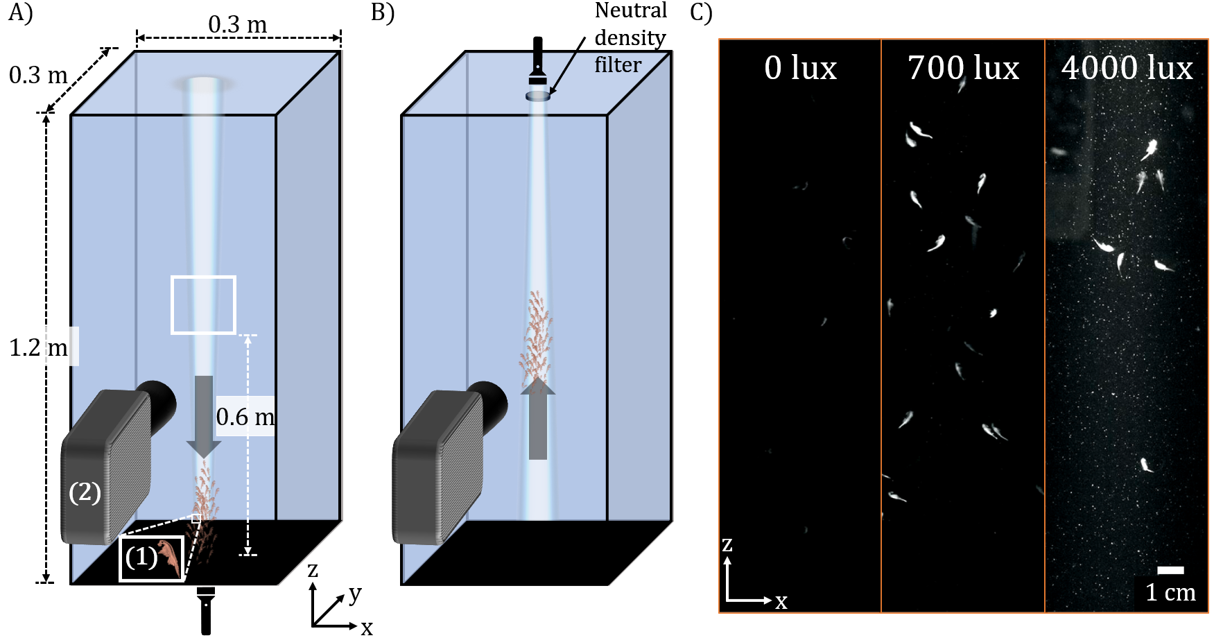
Figure 1: Schematic of experimental protocol for characterisation of phototactic response. A) A flashlight at the bottom of the tank was used to gather brine shrimp (1) at the bottom of a 1.2 m tall tank. B) The bottom flashlight was turned off, and the top flashlight was turned on inducing a vertical migration of swimmers. The light intensity of the top flashlight was adjusted using neutral density filters. Once the swimmers entered the field of view of the high-speed camera (2) a recording was started manually. C) Example frames captured of the x-z plane during vertical migrations with different neutral density filters and thus different light intensities. All trials were completed in the presence of an infrared tank illuminator, which was used alone in the 0 lux case. Three trials were conducted for each light intensity: 0, 800, 1500, 2300, and 4000 lumens per square metre (lux).

3.2 Individual swimmer response to background flow

To simulate vertical flows relevant to the behaviour of brine shrimp, water was drained from a 2.4 m tall tank with a cross section of 0.5 x 0.5 m, producing bulk flows in the range of 0.05-0.5 cm/s (figure 2). Before testing, the tank was filled with 10 $\mu$m silver-coated glass spheres (CONDUCT-O-FIL, Potters Industries, Inc.) to facilitate imaging of the flow field with a laser sheet. To confirm the quiescence of the tank, particle image velocimetry (PIV) was employed after introducing the animals with a 15 mL centrifuge tube. The tank was considered quiescent when the maximum time-averaged streamwise velocity was below 0.02 cm/s. Flow rate control was achieved using two series connected flow valves (1 inch NPT PVC Ball Valve), one for flow control and one for shut-off, and an inline flow metre (FLOMEC Flowmetre/Totalizer).

Once the tank was confirmed to be quiscent with PIV, a migration was induced with the same procedure explained in §3.1. A high-speed camera (Edgertronic SC1) was set up with a field of view of 21 x 26 cm (1024 x 1280 pixels), 90 cm up from the bottom of the tank. Once the first swimmer entered the camera field of view, the shut-off valve was manually opened to initiate the flow, and the camera was manually triggered to record for 30 seconds at 15 fps. Three trials were carried out for each of the five target speeds: 0, 0.07, 0.14, 0.21 and 0.3 cm/s. The trials were carried out on different days using different animals, considering the limited number of trials achievable with the volume of the tank.

To identify potential sources of measurement uncertainty, two significant factors were addressed. First, before the onset of the flow, a stream-wise velocity variation of 0.02 cm/s was allowed. Second, the flow speed was manually set using a ball valve and changed during each test due to variations in the height of the water column during draining. To address these uncertainties, an additional camera recorded flow rates displayed on the inline flow metre during each test. Both of these sources of variability were accounted for in the error bars of all flow measurements.

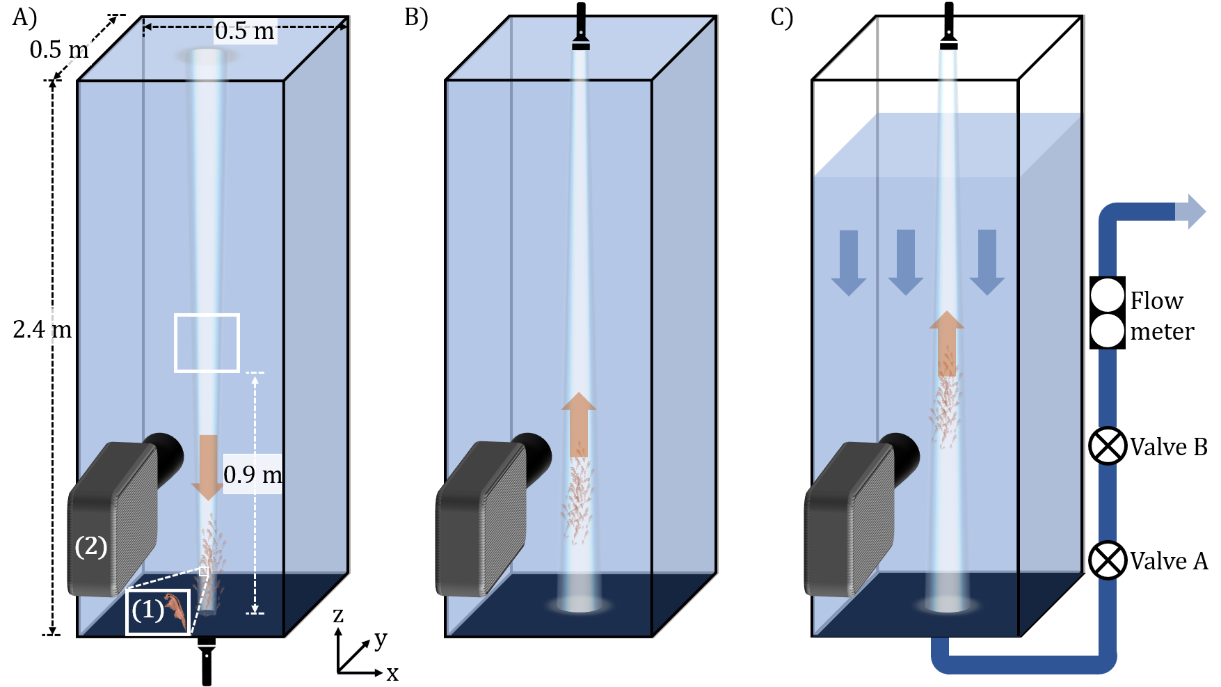
Figure 2: Schematic of experimental protocol for characterisation of flow response. A) A flashlight on the bottom of the tank was used to gather brine shrimp (1) at the bottom of a 1.2 m tall tank. B) The bottom flashlight was turned off and top flashlight was turned on inducing a vertical migration of swimmers. C) Once the swimmers entered the view of the high-speed camera (2) a flow valve was opened, exposing upward swimmers to bulk flow in the opposite direction of their motion and recording was started manually. Flow rate was set using a system of 2 flow valves and a flow meter in series. Three trials were conducted for each target speed: 0, 0.07, 0.14, 0.21 and 0.3 cm/s.

The captured videos of the vertical migration of brine shrimp were analysed using FIJI (Schindelin et al., 2012) and the wrMTrck plugin (Husson, 2012). The resulting swimming trajectories were fitted in MATLAB with a smoothing spline algorithm, which minimises a combination of squared residuals and curvature penalties utilising cubic smoothing spline interpolation to fit a curve to the provided data points. A smoothing parameter of 0.95 (figure 3) was selected to prioritise the reduction of oscillations, effectively smoothing out the fitted curve while preserving the overall trend of the data.

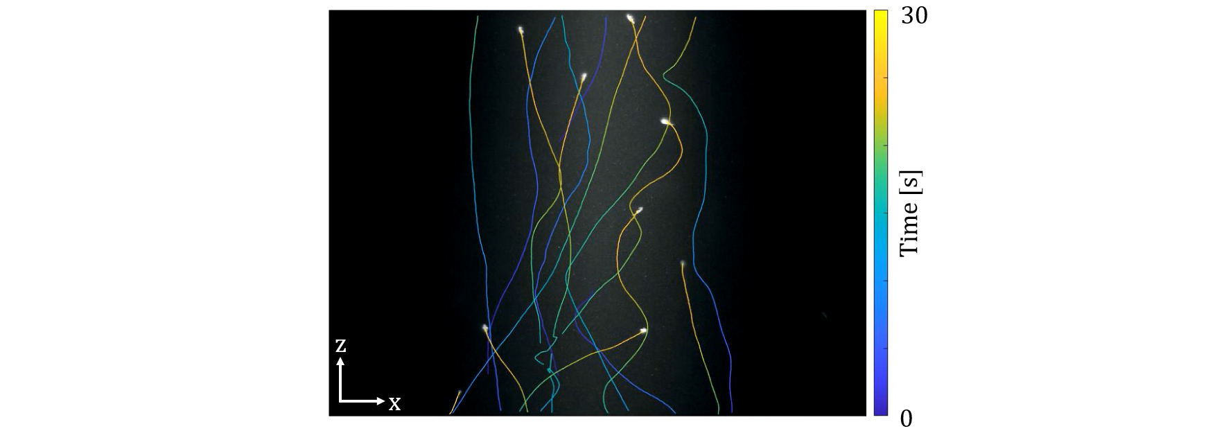
Figure 3: Plot of animal swimming trajectories from ImageJ wrMTrck over 30 seconds with the color indicating the swimmer position at each time.

3.3 Characterizing collective swimming

To reconstruct the 3D swimming trajectories of brine shrimp during induced vertical migration, a 3D Particle Tracking Velocimetry (PTV) method was used (figure 4), using scanning optics and a single high-speed camera (Photron FASTCAM SA-Z) (Fu et al., 2021). A 671 nm continuous wave laser (5-Watt Laserglow LRS0671 DPSS Laser System) was directed through a condenser lens (370 mm back focal length) and a sheet-forming glass rod by a mirror to ensure parallel beams. The distance between the laser plane and the high-speed camera was adjusted with a galvanometer (Thorlabs GVS211/M) controlled by a signal from an arbitrary function generator (Tektronix AFG3011C).

Each laser sheet sweep covered 6.6 cm of tank depth and took 0.1 seconds to complete. The high-speed camera captured three hundred two-dimensional (2D) 22 x 22 cm slices during this period. The scanned volume was centred on the tank cross section and positioned 0.9 m from the tank floor.

The experiments were carried out in the tank described in §3.1. The brine shrimp were added to the tank in densely packed ¼ teaspoons (approximately 125 swimmers) and 3 vertical migrations were induced as explained in §3.1 for each increment of swimmers added. Throughout vertical migration, the centre of the tank was scanned for 6 seconds every 50 seconds, totalling 7.5 minutes, to assess configuration changes over time.

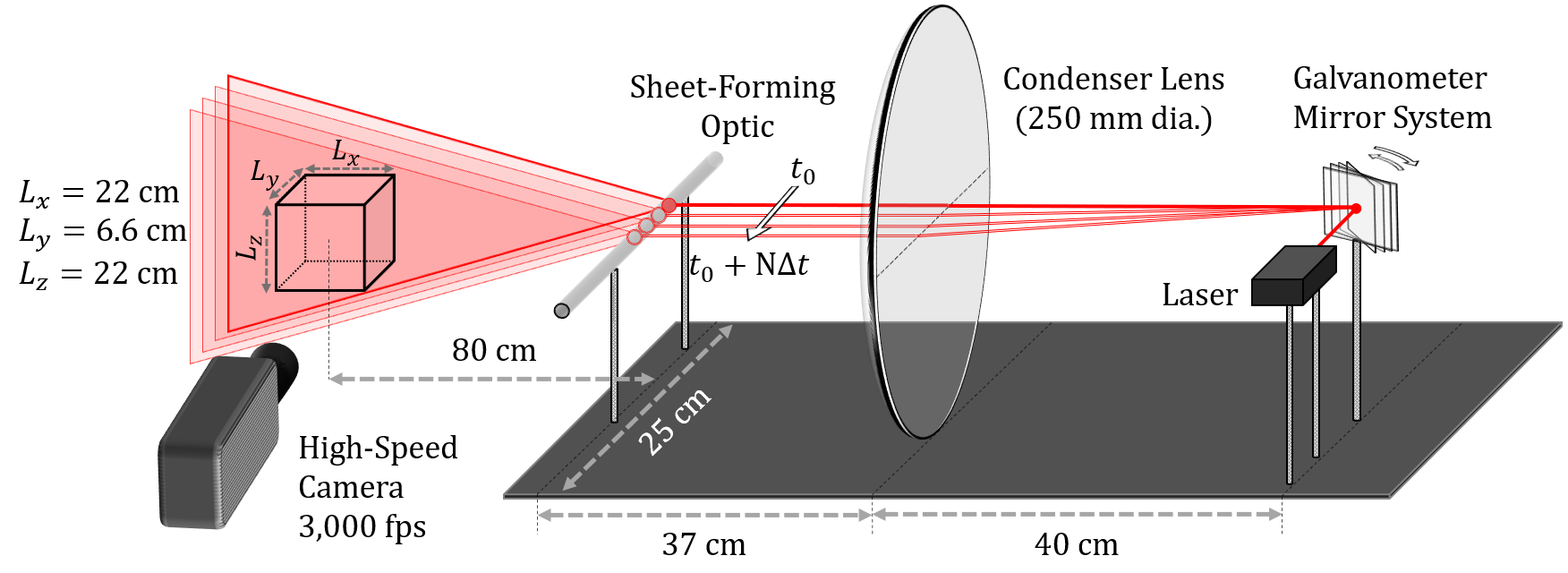
Figure 4: Diagram of the scanning system modified from Fu et al. (2021). Laser beam was directed at a mirror whose angle was controlled by a galvanometer. Following reflection by the mirror, the beam was passed through a condenser lens and glass rod in order to generate a laser sheet parallel to the camera field of view.

A 3D volume was constructed from 295 2D slices for each laser sweep (figure 5A) using a custom Matlab script, and the animal centroids were located using image processing tools. Then, a forward and backward nearest neighbour search in time was used to identify and label swimming trajectories (figure 5B).

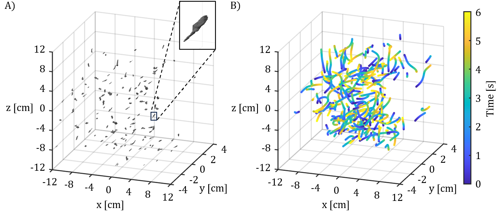
Figure 5: Volume reconstruction and animal tracking during an induced vertical migration in the positive z direction. A) 3D scanned reconstruction of 100 animal bodies. Close up of an individual animal shown for reference. B) Six second 3D swimming trajectories with color indicating the time at which the swimmer was at each position.

3.4 Modelling assimilation

3.4.1 Wake profile models

Two models for the individual wake structure were studied to explore the impact of local flow geometry on the aggregation-scale flow. The local flow was defined as a function of the radial distance, $r=\sqrt{x^{2}+y^{2}}$, and the characteristic width of the wake, $\sigma(z)$, at each value of z. First, a Gaussian model was implemented, consistent with the wake models previously used for wind turbine modelling:

$$\xi_{gaussian}\left(\frac{r}{\sigma(z)}\right)=e^{-\frac{r^{2}}{2\sigma(z)^{2}}}.$$ (9)

Second, a Ricker wavelet model was used to represent a local flow both in the direction of swimming and in the opposite direction of swimming:

$$\xi_{wavelet}\left(\frac{r}{\sigma(z)}\right)=-\left(1-\frac{r^{2}}{2\sigma(z)^{2}}\right)\>e^{-\frac{r^{2}}{3\sigma(z)^{2}}}.$$ (10)

These will be referred to as the Gaussian model and the wavelet model, respectively. The Gaussian model is commonly used in wind turbine modelling (Zong & Porté-Agel, 2020) and represents the flow behind the swimmer entirely downward. The modified Ricker wavelet is the equation for the second derivative of a Gaussian function, with a prefactor in the exponent denominator in order to create a function with a nonzero integral evaluation and allows for an annular region of downward flow (corresponding to the thrust generated by the legs) surrounding a region of upward flow (corresponding to drag of the body).

We modelled the spatial evolution of the propulsive jet as a self-similar, axisymmetric jet:

$$u_{s}=u_{0}\;c(z)\;\xi\left(\frac{r}{\sigma(z)}\right),$$ (11)

where $c(z)$ is a scaling factor and the shape of the wake is determined by $\xi(r/\sigma(z))$. An expression for $c(z)$ that conserves momentum by definition was derived by prescribing $u_{0}$, $\xi(r/\sigma(z))$, and $F_{z}$ (detailed steps provided in appendix A):

$$u_{s,gaussian}(x,y,z)=u_{0}\left(1-\sqrt{1+\frac{F_{z}}{\pi\rho\sigma(z)^{2}u_{0}^{2}}}\right)e^{-\frac{r^{2}}{2\sigma(z)^{2}}}.$$ (12)

$$u_{s,wavelet}(x,y,z)=u_{0}\left(\frac{4}{5}-\frac{4}{5}\sqrt{1+\frac{5F_{z}}{12\pi\rho\sigma(z)^{2}u_{0}^{2}}}\right)\left(-1\left(-\frac{r^{2}}{2\sigma(z)^{2}}\right)\>e^{-\frac{r^{2}}{3\sigma(z)^{2}}}\right),$$ (13)

Substituting the above equations 13 and 12 into 4 and integrating in the streamwise direction over a circular cross section with infinite radius, the expressions for $u_{c}$ is obtained:

$$u_{c,gaussian}(z)=\frac{u_{0}}{2}\left(1+\sqrt{1+\frac{F_{z}}{\pi\rho\sigma(z)^{2}u_{0}^{2}}}\right).$$ (14)

$$u_{c,wavelet}(z)=\frac{u_{0}}{2}\left(1+\sqrt{1+\frac{5F_{z}}{12\pi\rho\sigma(z)^{2}u_{0}^{2}}}\right),$$ (15)

A swimmer moving vertically at constant velocity must overcome the negative buoyancy that arises from the swimmer having a greater density than sea water. The balance of force on the swimmer is expressed as follows:

$$F_{thrust}=gV_{s}(\rho_{s}-\rho)$$ (16)

The thrust is introduced over some distance and not at an exact point in the flow. Therefore, we amended this expression to:

$$F_{thrust}(z)=gV_{s}(\rho_{s}-\rho)\frac{1+\operatorname{erf}\frac{z}{L_{s}}}{2},$$ (17)

for a more gradual development of the wake, where $L_{s}$ is the length of the swimmer’s body length. Similarly, an empirical model for the effective diameter of the wake as a function of the streamwise distance from the swimmer was used to capture the wake expansion:

$$\sigma(z)=0.25+0.25\ \text{log}(1+e^{(z-1.5)/L_{s}})$$ (18)

The variables explicitly defined for the analytical model are listed in table 1. These values were approximated to be on the order of observations made during lab experiments using brine shrimp. We used $L_{s}$, the body length of a swimmer, to normalize computational experiments and results.

Symbol	Variable	Value	Unit
$U_{\infty}$	swimming velocity	1	cm/s
$g$	gravitational acceleration	9.8	m/s2
$V_{s}$	swimmer volume	$0.3\pi$	cm3
$\rho_{s}$	swimmer density	1055	kg/m3
$\rho$	seawater density	1025	kg/m3
$L_{s}$	body length	1	cm

Table 1: Variables used in wake superposition model for induced flow in vertical migration.

3.4.2 Computational experiments

Computational experiments were designed to examine the impact of aggregate characteristics on induced flow. First, changes due to group length were examined. The length of the group was increased in each test, while animal number density and width remained constant (table 2A). To maintain constant animal number density and width of the group, the number of swimmers increased linearly with increasing length of the group. Second, to test the impact of animal number density on the resulting flow, the number of swimmers and the length of the group were kept constant while increasing the cross-sectional area in the spanwise dimensions (table 2B). This resulted in an animal number density that decreased with increasing width as 1/width². For each experiment with a selected set of parameters, 3 iterations of swimmers were placed randomly with these specifications while maintaining a minimum nearest neighbour distance of 1 body length.

A)	Length tests
Test	Number (N)	Length (L)	Width (W)	Number density
Units	swimmers	body length	body length	swimmers/body length3
1	40	4	5	0.4
2	100	10	5	0.4
3	200	20	5	0.4
4	400	40	5	0.4
5	520	52	5	0.4

B)	Animal number density tests
Test	Number (N)	Length (L)	Width (W)	Number density
Units	swimmers	body length	body length	swimmers/body length3
1	100	20	2.2	1
2	100	20	3	0.6
3	100	20	4	0.3
4	100	20	7	0.1
5	100	20	10	0.05
6	100	20	19	0.01

Table 2: Parameters to be examined are the number of swimmers in the group, $N$, the length of the group, $L$, and the width of the group, $W$. Together, these three parameters result in a group metric that we refer to as the animal number density, measured in animals per body length³ and calculated as $N/(W^{2}L)$. These parameters are used to experiment with changes in A) group length, and B) animal number density.

4 Results

4.1 Swimmer response to light and background flow

Swimmers involved in vertical migration patterns are subject to varying degrees of light exposure and background flow, influenced by the presence of upstream swimmers that obstruct the light source and create wakes. However, brine shrimp consistently maintained swimming speeds irrespective of flow conditions and light intensities tested (figure 6). Consequently, in subsequent modelling experiments, swimmers were posited to maintain constant velocity.

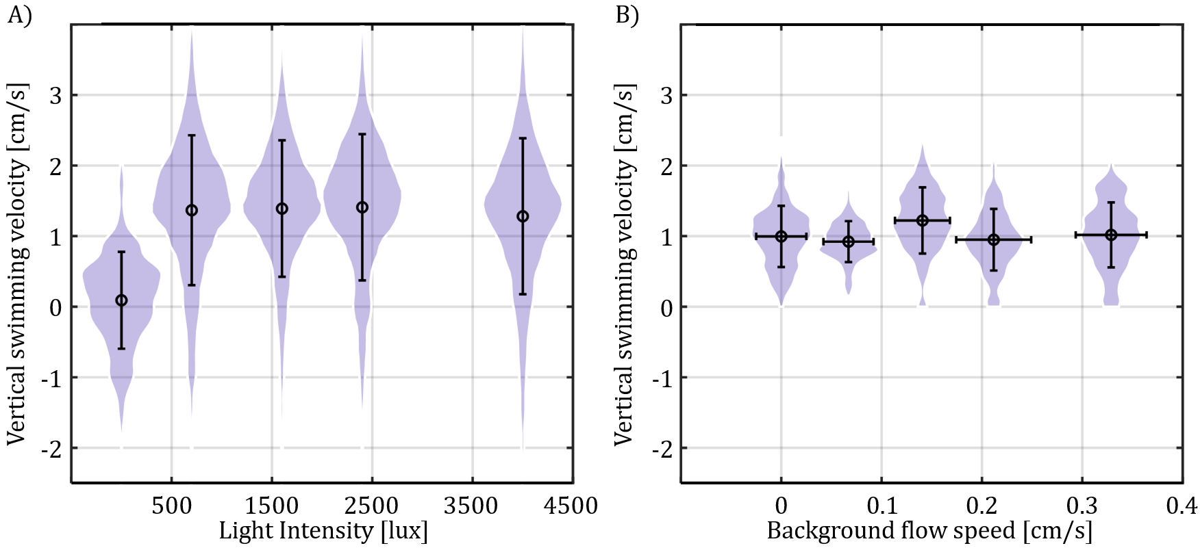
Figure 6: Brine shrimp maintain a constant velocity with environmental changes. A) Vertical swimming speed as a function of lumens per square metre (lux). Infrared lamp only shown as a control, 0 lux. B) Vertical swimming speed as a function of background flow. Horizontal error bars represent range of flows experienced.

4.2 Collective swimming dynamics

As the number of swimmers within the scanned volume increases, the average nearest neighbor distance decreases but reaches a limit, evidence of exclusion zones (figure 7). To determine the asymptotic limit of the data, we employed the MATLAB fit function to determine the best-fit power law relationship between animal number density, $x$, and the average nearest neighbor distance, $y$). The power law fit was calculated as $y=a+\frac{b}{cx^{d}}$. This approach allowed us to investigate how the average nearest neighbor distance converges as the animal number density increases. The asymptote value, $a$, of the fit was found to be 1.16. Consequently, we approximated the minimum space between swimmers for modelling purposes to be 1 cm.

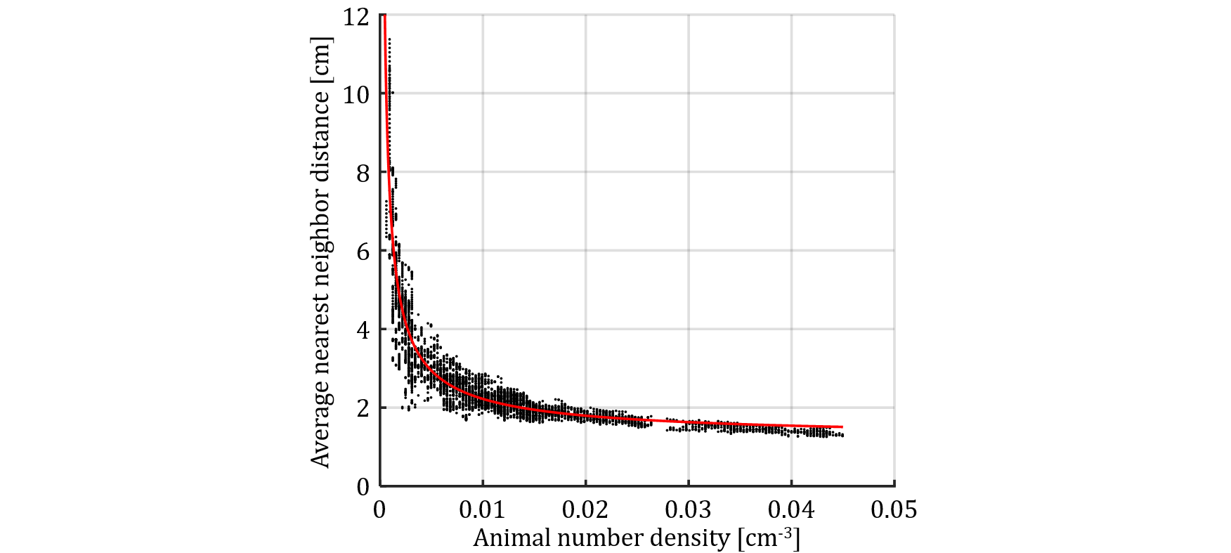
Figure 7: Changes in average nearest neighbour distance during an induced vertical migration with increasing number of brine shrimp within the scanned volume. Power law best fit plotted in red, $y=1.16+\frac{-0.02}{-0.64x^{0.74}}$, with $R^{2}$ value of 0.85.

4.3 Modelled collective hydrodynamics

The variables derived experimentally above were incorporated into the analytical model to characterise the collectively induced flow. All calculations were done in the swimmer-fixed reference frame. However, for the sake of clarity, the results presented here are depicted and discussed in the lab-fixed frame.

4.3.1 Dependence on aggregation size

In our first experiment, we examine the flow induced by groups with the same animal number density, 0.4 animals per body length³ but different lengths (figure 8). Three trials of each group length were generated with randomly placed swimmers. The average convection velocity and standard deviation of each group length was plotted (figure 9). The convection velocity generated within the groups were found to overlap each other. This indicated that the upstream portion of the flow generated within a group was not affected by the downstream flow. Furthermore, the induced flow ceased to exhibit a discernible dependence on the group length beyond a certain threshold, estimated at around 20-30 body lengths in this case. Consequently, we found that the dynamics of both longer and shorter groups can be approximated by studying the flow generated by any group longer than this threshold length.

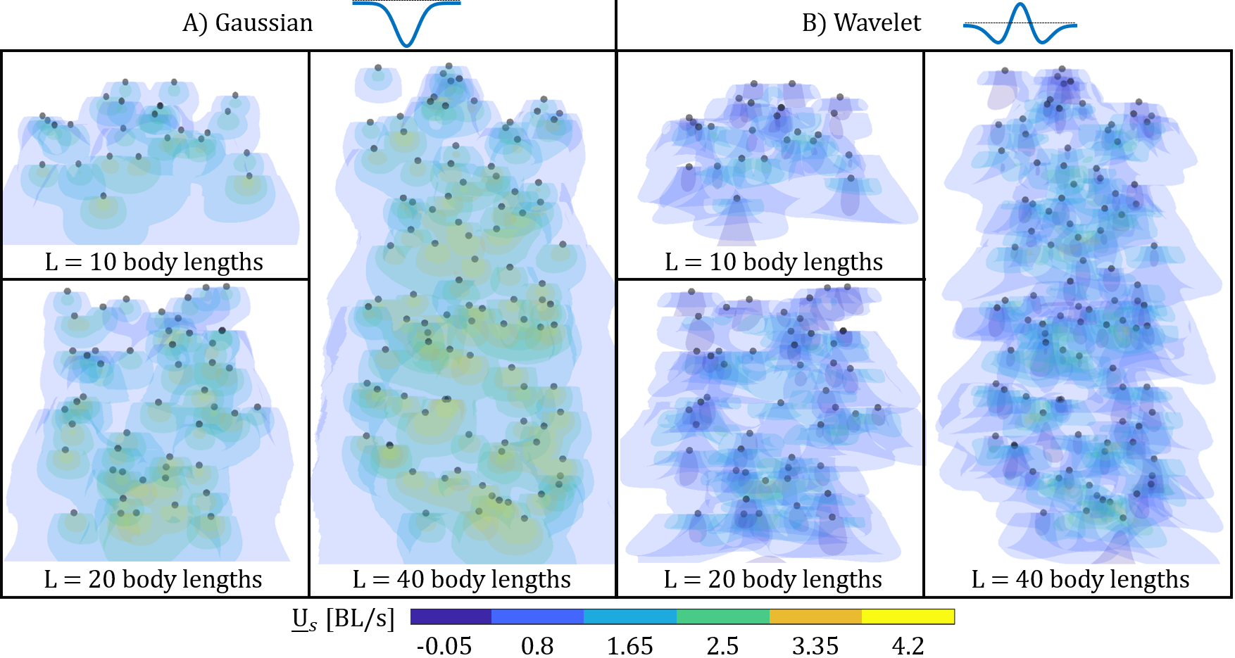
Figure 8: 2D projection of group geometry and induced flow contour map are shown for groups with an animal number density of 0.2 animals per body length³ with increasing group length. Black spheres are used to show the positions of swimmers. Five isosurfaces of the 3D flow field output generated from the analytical model are superimposed with the color indicating the flow magnitude. Results are shown side by side from A) the wavelet model and B) the Gaussian model.

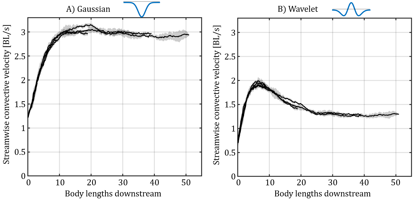
Figure 9: Lab frame convection velocity, $U_{c}(z)-U_{\infty}$ measured in body lengths per second, within the collective plotted against streamwise distance from start of group, $z$. Each line shown as the average with shaded standard deviation based on 3 randomised iterations. Five group lengths: 4, 10, 20, 40, and 52 body lengths, are superimposed on top of each other using A) the Gaussian model and B) the wavelet model.

4.3.2 Dependence on swimmer spacing

In our second experiment, we investigate the influence of swimmer spacing on the flow generated by the collective. We randomly placed 100 swimmers within a volume of constant length but varying widths, resulting in changes in animal number densities (figure 10). Three trials were initiated for each case. Our findings reveal a positive correlation between induced convective flow and animal number density (Figure 11). Specifically, for groups with animal number densities exceeding 0.05 animals per body length³ using the Gaussian model, a consistent trend emerged: the flow increased steadily with length until reaching a threshold length, beyond which the dependence on length decreased to a near-stable state. Groups with animal number densities below 0.05 animals per body length³ with the Gaussian model and all number densities for the wavelet model exhibited peak flow early in the aggregation process, followed by substantial decreases in flow, sometimes to a flow lower than that generated at the beginning of the aggregation. In these cases, the flow still reached a threshold length, after which the dependence of flow on length diminished.

We also observe that in many cases the estimated convection velocity exceeds the velocity prescribed to swimmers in this model, which was set at 1 body length/second. Although this model captures an instantaneous snapshot in time for a specific configuration of swimmers, in reality, swimmers facing a flow exceeding 1 body length/second would be pushed in the opposite direction to their swimming motion. Thus, these configurations are paradoxical since we have initialised a configuration of swimmers that creates a flow that would make this animal number density impossible to maintain.

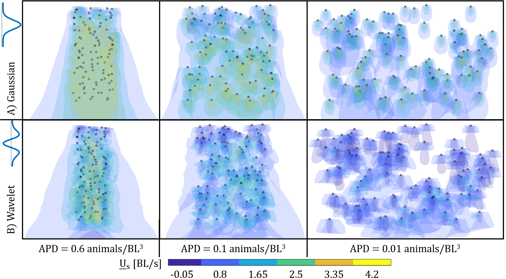
Figure 10: 2D projection of group geometry and induced flow contour map for 100 swimmers with increasing group width, resulting in decreasing animal number density. Black spheres are used to show the positions of swimmers. Five isosurfaces of the 3D flow field output generated from the analytical model are superimposed with the color indicating the flow magnitude. Results are shown side by side from A) the wavelet model and B) the Gaussian model.

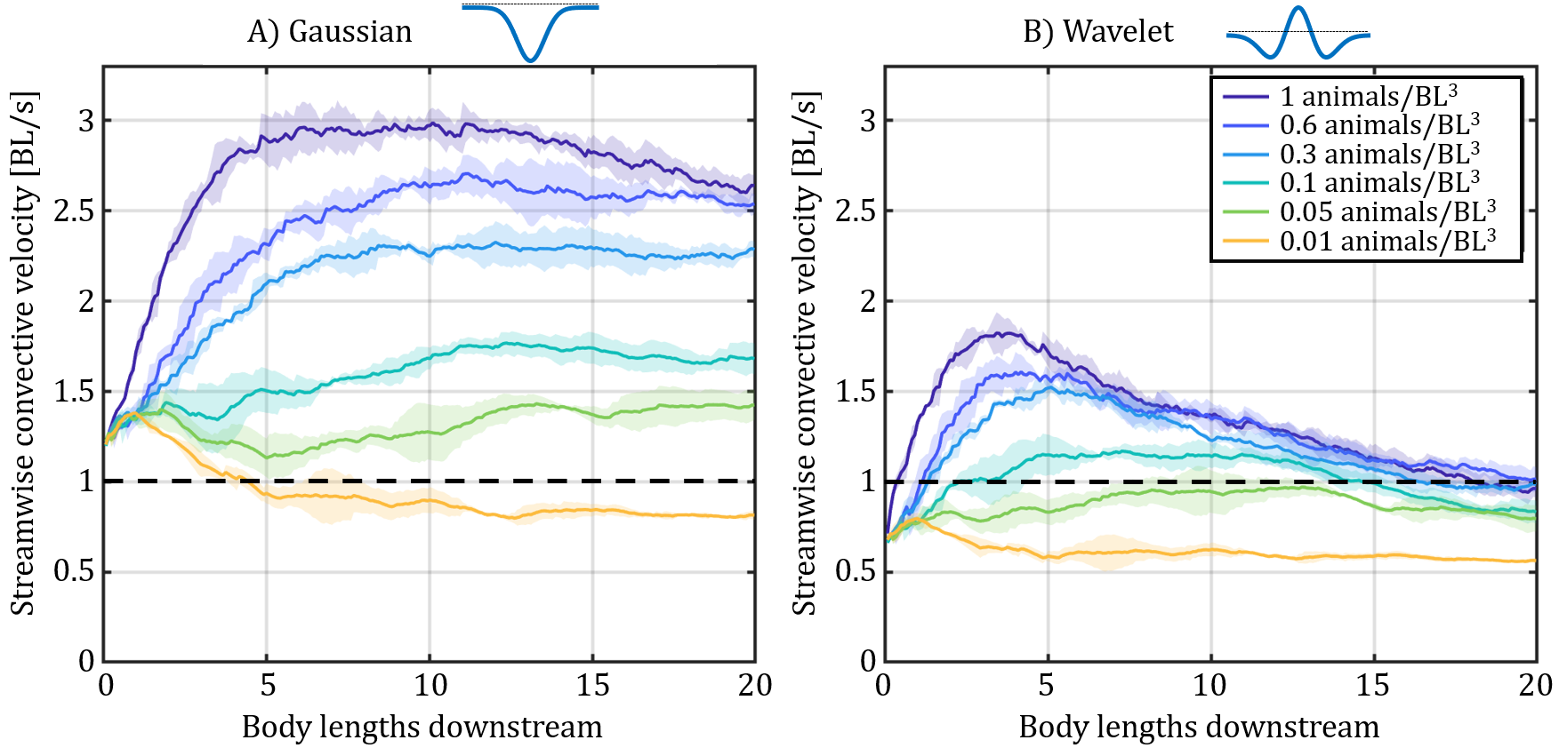
Figure 11: Lab frame convection velocity, $U_{c}(z)-U_{\infty}$ measured in body lenghts per second, within the collective plotted against streamwise distance from start of group, $z$. Each line shown as the average with shaded standard deviation based on 3 randomized iterations. Six animal number densities, 0.01, 0.05, 0.1, 0.3, 0.6, and 1 animal per body length³ are plotted with A) the Gaussian model and B) the wavelet model. Dashed line is added to show the swimming speed prescribed in the model, 1 body length per second

To further investigate the stability of the aggregation, we analysed the flow experienced by individual swimmers within the collective. The distribution of flow velocities for varying animal number densities (figure 12) revealed that a significant proportion of swimmers in groups denser than 0.1 animals per body length³ experience a flow exceeding 1 body length per second. The magnitude and range of these flows experienced, especially in denser groups, indicate an unsustainable configuration. However, it is also important to note that the experienced flows may vary based on the position within the swarm, contributing to the range of flow velocities observed among swimmers.

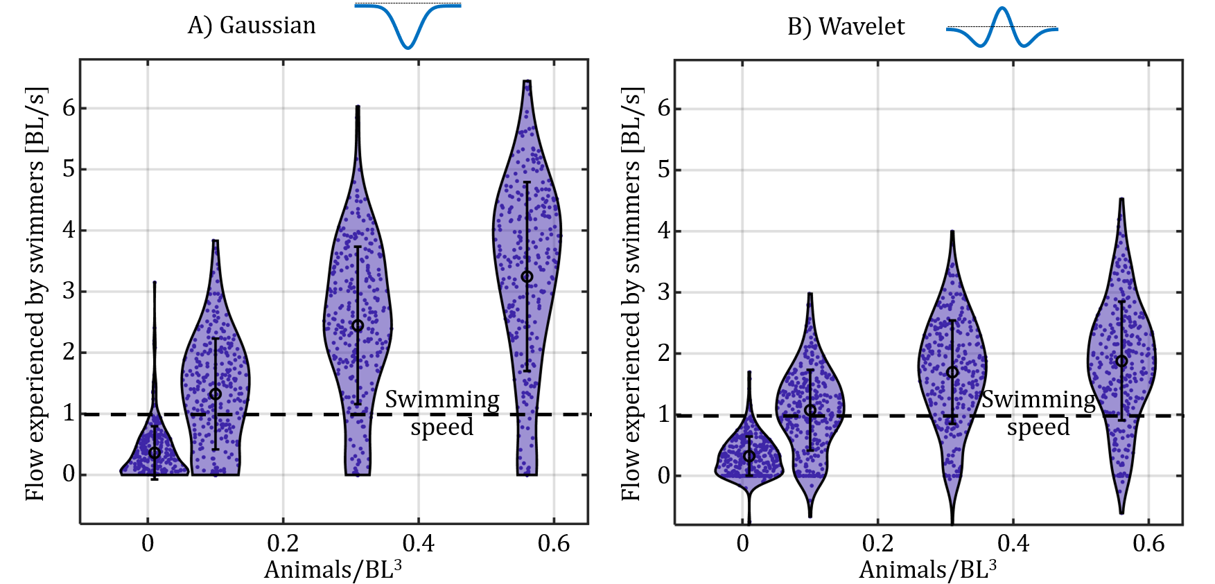
Figure 12: Distribution of flow experienced by swimmers, $u_{0}^{i}-U_{\infty}$, at different animal number densities using A) the Gaussian model and B) the wavelet model.

4.3.3 Dependence on relative swimmer position

Therefore, we proceeded to investigate how the positioning of individual swimmers within the group affects the flow experienced by them. Analysing three trials of the case of 0.6 animals per body length³, we observed that swimmers positioned closer to the centre of the group encountered progressively higher induced flow velocities (figure 13).

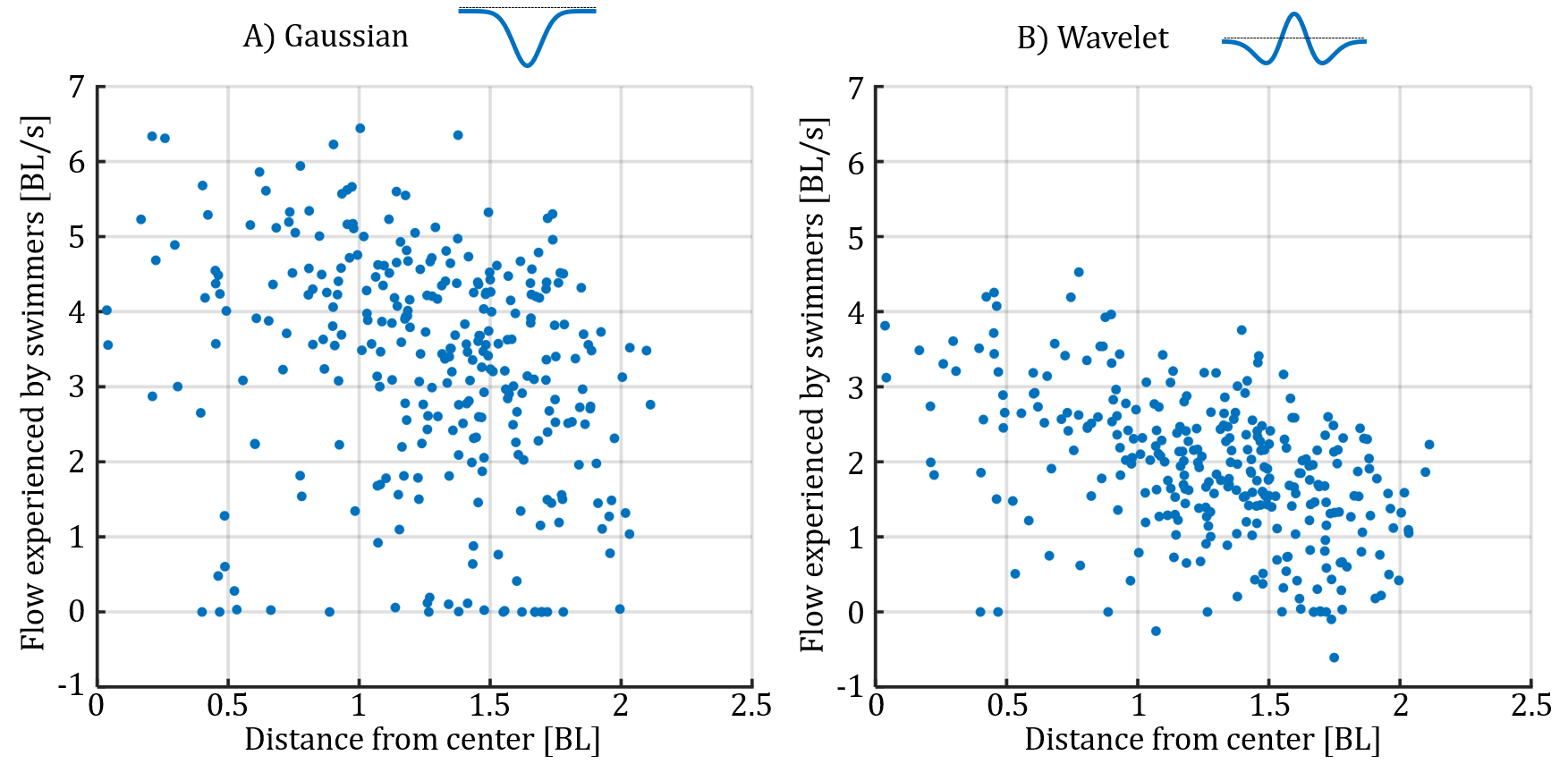
Figure 13: Flow experienced by individual swimmers, $u_{0}^{i}-U_{\infty}$ as a function of radial distance from the centre of the group, $r=\sqrt{x^{2}+y^{2}}$. Data shown from the 3 randomised trials of 100 swimmers with 0.6 animals per body length³.

Next we studied the flow experienced by swimmers as a function of distance from the start of the group. Using the same three trials of the 0.6 animals per body length³ case, we observed that swimmers positioned closer to the start of the group encountered lower flow velocities (figure 14).

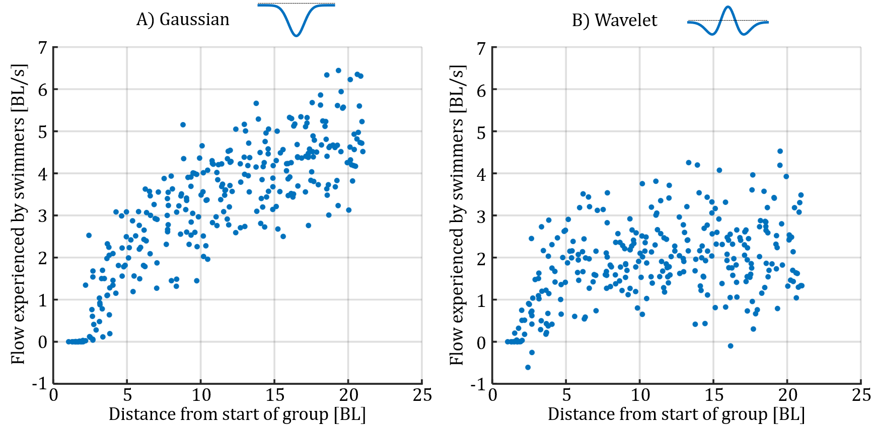
Figure 14: Flow experienced by individual swimmers, $u_{0}^{i}-U_{\infty}$ as a function of distance from the start of the group, $z$. Data shown from the 3 randomised trials of 100 swimmers with 0.6 animals per body length³.

In all previous computational experiments, the swimmers were randomly placed with specified parameters. To provide context to these findings, we conducted a final test by initialising the computational model with a swimmer configuration obtained by 3D PTV of induced brine shrimp migrations from the previous section. We used an case in which 100 brine shrimp were scanned and reconstructed within the volume ($L$= 22 cm, $W_{1}$= 6.6 cm, $W_{2}$= 22 cm), resulting in an animal number density of 0.03 animals/cm³ (figure 15). The flow derived from the experimentally obtained swimmer configuration resulted in a higher convection magnitude than the 0.05 animals/cm³ animal number density randomised experiment, although the experimental configuration was sparser (figure 16). However, it should be noted that we observed a denser pack of swimmers in the centre of the migration compared to the outer region. Therefore, a portion of this difference can be attributed to the animal number density being overly generalised and not capturing spatial variations in the configuration.

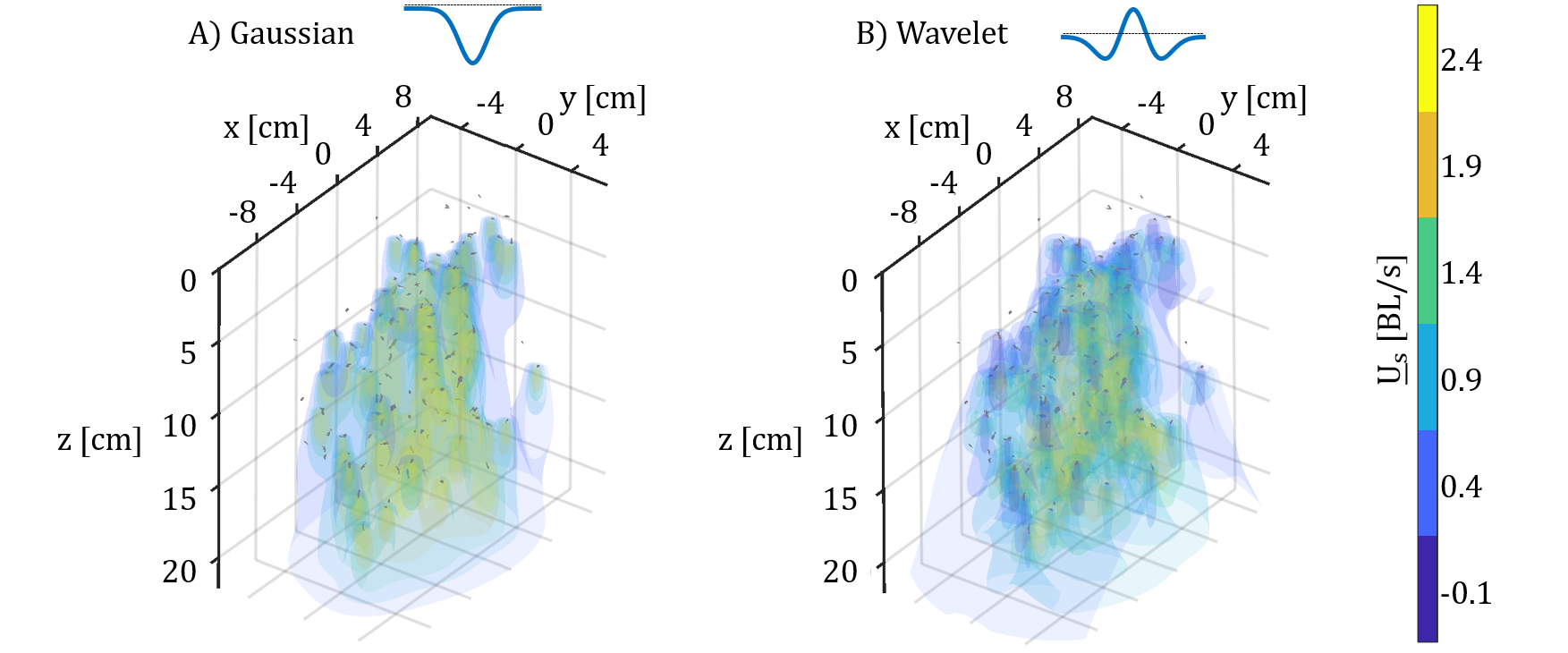
Figure 15: Scanned and reconstructed brine shrimp from 3D PTV overlayed with flow field, $U_{s}(x,y,z)$ generated by A) the Gaussian wake model and B) the wavelet wake model.

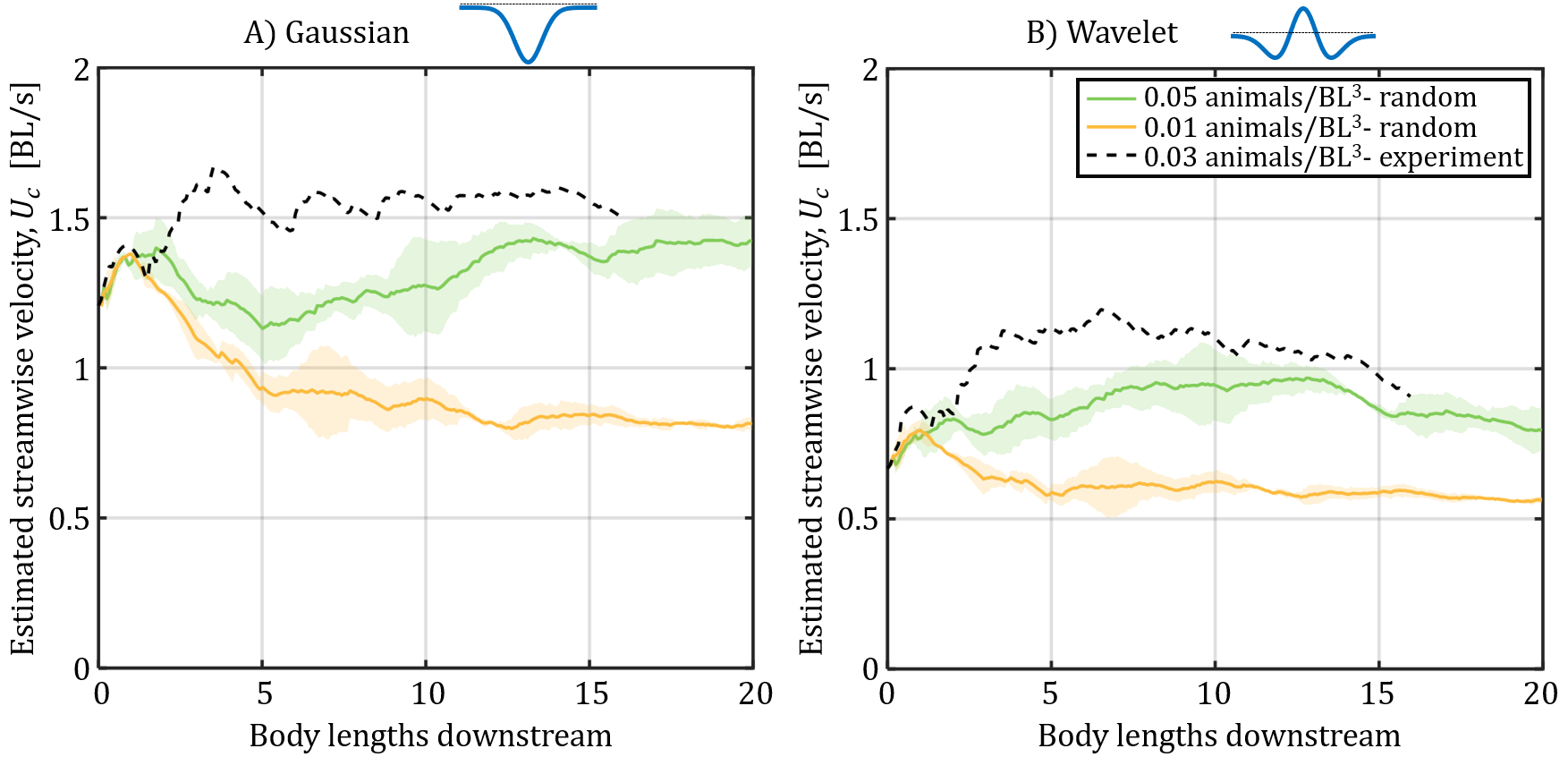
Figure 16: Comparing convective veloicty generated by randomly distributed swimmer locations and experimentally initialised swimmer locations. Estimated convection velocity plotted against streamwise distance from start of group, $z$ for randomised computational experiments and for a model initialised with locations of brine shrimp during induced vertical migration using A) the Gaussian model and B) the wavelet model.

5 Discussion

We have developed an analytical wake superposition model for groups of hydrodynamically interacting organisms. This model was implemented numerically with parameters derived from empirical observations of brine shrimp, incorporating observed responses to light and flow as well as 3D swimming trajectories. Computational experiments with this model produce a 3D flow field and an estimated convection velocity. This analytical model provides a quantitative framework for understanding hydrodynamic interactions within swimming aggregations at intermediate Reynolds numbers.

Our findings highlight the intricate interplay between wake kinematics, swimmer spacing, and overall group size and arrangement in inducing flows within swimming collectives. Notably, the wavelet wake model, when compared to the Gaussian wake model, generates lower-magnitude convective velocities, resulting in swimmers within the group experiencing slower flows. The positive flow regions in the wavelet have an annular shape with the maximum flow value reached over a circle in space. In contrast, the Gaussian wake reaches a maximum value at a single point. Thus, the wavelet model has a more spread-out region of positive flow. In addition, the negative flow region was averaged when looking at the convective velocity. The differences between the flow induced by Gaussian and wavelet wake models exemplify the importance of local flow kinematics and thus motivate continuing work to measure and model individual organism-level flows.

By comparing groups of different lengths, we found that the flow within the group exhibits decreased sensitivity to the length of the group beyond a threshold. With a uniform distribution of swimmers, there was a constant infusion of momentum to the flow with streamwise distance from the start of the group. However, the velocity of the induced flow increases within the group length only until the mass flux term of the momentum balance dominates, and each individual adds less velocity to the flow than those upstream. The impact of this added velocity decreases further with diffusion before reaching downstream swimmers. In addition, we found that the upstream portion of the flow within the group was not affected by the group downstream. Thus the dynamics of shorter groups can be extracted from the dynamics of groups longer than a certain threshold.

Experimenting with group densities, we found that the collective convective velocity increased with the animal number density. Dense configurations resulted in flows that exceeded the swimming speed of the organism, resulting in unstable structures. This observation raises questions about the apparent stability of swimmer aggregations in field observations, where these high-density configurations are known to persist. The contrast between experimental results and observed natural behaviour prompts inspiration for future model improvements to explore mechanisms used by organisms to navigate and thrive in environments characterised by dynamic collective swimming. For example, there is evidence that animals exploit fluid structures to improve locomotion (Weber et al., 2020; Oteiza et al., 2017). In the present study, all experiments were initialised with randomly placed swimmers in a prescribed volume swimming directly upward. The only constraint in swimming placement was the exclusion zones that maintain a minimum nearest neighbour distance. If the model included some parameters to actively optimise swimmer placement, downstream swimmers might exploit the drag region within the wavelet model, which provides flow in the desired swimming direction. Continued work to study the stability of these systems could incorporate discrete time-step dynamics to investigate how collective flow-inducing systems evolve.

This model is highly adaptable to different wake profiles and aggregation configurations, allowing future exploration of flows generated by other organisms with different wake profiles and collective behaviours. Furthermore, this model is applicable across a spectrum of ecological and engineering contexts, including active and passive particle systems such as marine snow and multiphase flows.

Appendix A

We model the spatial evolution of the propulsive jet as a self-similar, axisymmetric jet:

$$u_{s}=u_{0}\;c(z)\;\xi\left(\frac{r}{\delta(z)}\right).$$ (19)

In the following derivation $u_{0}$, $\xi(r/\delta(z))$, and $F_{z}$ are prescribed, and 19 is plugged into simplified momentum:

$$F_{z}=\rho\iint_{wake}{u_{w}(x,y,z)}u_{s}(x,y,z)\;dxdy,$$ (20)

to arrive at:

$$F_{z}=\rho\iint u_{0}^{2}\;\left(c(z)\;\xi(r,z)-\left[c(z)\;\xi(r,z)\right]^{2}\right)\;drd\theta,$$ (21)

to derive an expression for $c(z)$ that conserves momentum by definition. Next, $\xi(r/\delta(z))$ is defined as follows for each of the two wake models, and $\delta(z)$ is defined to be the standard deviation at each value of z, $\sigma(z)$. Note that when these functions are used in signal processing and analysis, a normalised version is used, ensuring that the total energy or power is conserved across different scales, which is important for accurate signal analysis. In this derivation, the prefactor $c(z)$ is constructed to conserve momentum directly, negating the need for commonly used normalisation prefactors. To solve for $c_{g}(z)$ and $c_{w}(z)$, the prefactors for the Gaussian and wavelet wake models, respectively, the two wake shapes:

$$\xi_{gaussian}\left(\frac{r}{\sigma(z)}\right)=e^{-\frac{r^{2}}{2\sigma(z)^{2}}},$$ (22)

$$\xi_{wavelet}\left(\frac{r}{\sigma(z)}\right)=-\left(1-\frac{r^{2}}{2\sigma(z)^{2}}\right)\>e^{-\frac{r^{2}}{3\sigma(z)^{2}}}$$ (23)

are substituted into 21:

$$F_{z}=\rho\iint u_{0}^{2}\;\left(c_{g}(z)e^{-\frac{r^{2}}{2\sigma(z)^{2}}}-\left(c_{g}(z)e^{-\frac{r^{2}}{2\sigma(z)^{2}}}\right)^{2}\right)\;drd\theta,$$ (24)

$$F_{z}=\rho\iint u_{0}^{2}\;\left(c_{w}-\left(1-\frac{r^{2}}{2\sigma(z)^{2}}\right)\>e^{-\frac{r^{2}}{3\sigma(z)^{2}}}-\left(c_{w}(z)-\left(1-\frac{r^{2}}{2\sigma(z)^{2}}\right)\>e^{-\frac{r^{2}}{3\sigma(z)^{2}}}\right)^{2}\right)\;drd\theta$$ (25)

and then integrated in the streamwise direction over a circular cross section with infinite radius. For each shape, there are 2 solutions for $c(z)$. We select the solution that is negative and tends to 0 with increasing positive z values:

$$c_{g}(z)=1-\sqrt{1+\frac{F_{z}}{\pi\rho\sigma(z)^{2}u_{0}^{2}}},$$ (26)

$$c_{w}(z)=\frac{4}{5}-\frac{4}{5}\sqrt{1+\frac{5F_{z}}{12\pi\rho\sigma(z)^{2}u_{0}^{2}}}.$$ (27)

Combining 22 with 26 and 23 with 27 and plugging into 19 to derive the final expressions for $u_{s}$:

$$u_{s,wavelet}(x,y,z)=u_{0}\left(\frac{4}{5}-\frac{4}{5}\sqrt{1+\frac{5F_{z}}{12\pi\rho\sigma(z)^{2}u_{0}^{2}}}\right)\left(-1\left(-\frac{r^{2}}{2\sigma(z)^{2}}\right)\>e^{-\frac{r^{2}}{3\sigma(z)^{2}}}\right),$$ (28)

$$u_{s,gaussian}(x,y,z)=u_{0}\left(1-\sqrt{1+\frac{F_{z}}{\pi\rho\sigma(z)^{2}u_{0}^{2}}}\right)e^{-\frac{r^{2}}{2\sigma(z)^{2}}}.$$ (29)

Finally, substituting the above equations 28 and 29 into the wake convection velocity, $u_{c}$:

$${u_{c}(z)}=\frac{\displaystyle\iint_{wake}{u_{w}(x,y,z)}u_{s}(x,y,z)\;dxdy}{\displaystyle\iint_{wake}u_{s}(x,y,z)\;dxdy},$$ (30)

we arrive at:

$$u_{c,wavelet}(z)=\frac{u_{0}}{2}\left(1+\sqrt{1+\frac{5F_{z}}{12\pi\rho\sigma(z)^{2}u_{0}^{2}}}\right),$$ (31)

$$u_{c,gaussian}(z)=\frac{u_{0}}{2}\left(1+\sqrt{1+\frac{F_{z}}{\pi\rho\sigma(z)^{2}u_{0}^{2}}}\right).$$ (32)

References

- Bandara et al. (2021) Bandara, K., Varpe, Ø., Wijewardene, L., Tverberg, V. & Eiane, K. 2021 Two hundred years of zooplankton vertical migration research. Biological Reviews 96 (4), 1547–1589.
- Berlinger et al. (2021) Berlinger, F., Gauci, M. & Nagpal, R. 2021 Implicit coordination for 3d underwater collective behaviors in a fish-inspired robot swarm. Science Robotics 6.
- Brady & Bossis (1988) Brady, J. F. & Bossis, G. 1988 Stokesian dynamics. Annual Review of Fluid Mechanics 20 (1), 111–157.
- Crespo et al. (1999) Crespo, A., Hernández, J. & Frandsen, S. 1999 Survey of modelling methods for wind turbine wakes and wind farms. Wind Energy 2 (1), 1–24.
- Dabiri (2005) Dabiri, J. O. 2005 On the estimation of swimming and flying forces from wake measurements. Journal of Experimental Biology 208 (18), 3519–3532.
- Derr et al. (2022) Derr, N. J., Dombrowski, T., Rycroft, C. H. & Klotsa, D. 2022 Reciprocal swimming at intermediate reynolds number. Journal of Fluid Mechanics 952, A8.
- Dewar et al. (2006) Dewar, W., Bingham, R., Iverson, R., Nowacek, D., Laurent, L. & Wiebe, P. 2006 Does the marine biosphere mix the ocean? Journal of Marine Research 64.
- Eldredge (2007) Eldredge, J. D. 2007 Numerical simulation of the fluid dynamics of 2d rigid body motion with the vortex particle method. Journal of Computational Physics 221 (2), 626–648.
- Farmer et al. (1987) Farmer, D. D., Crawford, G. B. & Osborn, T. R. 1987 Temperature and velocity microstructure caused by swimming fish1. Limnology and Oceanography 32 (4), 978–983.
- Fernández Castro et al. (2022) Fernández Castro, B., Peña, M., Nogueira, E., Gilcoto, M., Broullón, E., Comesaña, A., Bouffard, D., Naveira G., Alberto C. & Mouriño-Carballido, B. 2022 Intense upper ocean mixing due to large aggregations of spawning fish. Nature Geoscience 15 (44), 287–292.
- Fu et al. (2021) Fu, M. K., Houghton, I. A. & Dabiri, J. O. 2021 A single-camera, 3d scanning velocimetry system for quantifying active particle aggregations. Experiments in Fluids 62 (8), 168.
- Gregg & Horne (2009) Gregg, M. C. & Horne, J. K. 2009 Turbulence, acoustic backscatter, and pelagic nekton in monterey bay. Journal of Physical Oceanography 39 (5), 1097–1114.
- Houghton et al. (2018) Houghton, I. A., Koseff, J. R., Monismith, S. G. & Dabiri, J. O. 2018 Vertically migrating swimmers generate aggregation-scale eddies in a stratified column. Nature 556, 497–500.
- Huntley & Zhou (2004) Huntley, M. E. & Zhou, M. 2004 Influence of animals on turbulence in the sea. Marine Ecology Progress Series 273, 65–79.
- Husson (2012) Husson, S. J. 2012 Keeping track of worm trackers. WormBook p. 1–17.
- Ishikawa et al. (2006) Ishikawa, T., Simmonds, M. P. & Pedley, T. J. 2006 Hydrodynamic interaction of two swimming model micro-organisms. Journal of Fluid Mechanics 568, 119–160.
- Katic et al. (1987) Katic, I., Højstrup, J. & Jensen, N. O. 1987 A simple model for cluster efficiency. EWEC 1, 407–410.
- Katija (2012) Katija, K. 2012 Biogenic inputs to ocean mixing. Journal of Experimental Biology 215 (6), 1040–1049.
- Ko et al. (2023) Ko, H., Lauder, G. & Nagpal, R. 2023 The role of hydrodynamics in collective motions of fish schools and bioinspired underwater robots. Journal of The Royal Society Interface 20 (207), 20230357.
- Lauder & Madden (2008) Lauder, G. V. & Madden, P. G. A. 2008 Advances in comparative physiology from high-speed imaging of animal and fluid motion. Annual Review of Physiology 70 (1), 143–163.
- Lauga & Powers (2009) Lauga, E. & Powers, T. R. 2009 The hydrodynamics of swimming microorganisms. Reports on Progress in Physics 72 (9), 096601.
- Lin et al. (2011) Lin, Z., Thiffeault, J. & Childress, S. 2011 Stirring by squirmers. Journal of Fluid Mechanics 669, 167–177.
- Lissaman (1979) Lissaman, P. B. S. 1979 Energy effectiveness of arbitrary arrays of wind turbines. Journal of Energy 3 (6), 323–328.
- Mathijssen et al. (2019) Mathijssen, A. J. T. M., Culver, J., Bhamla, M. S. & Prakash, M. 2019 Collective intercellular communication through ultra-fast hydrodynamic trigger waves. Nature 571, 560–564.
- Oteiza et al. (2017) Oteiza, P., Odstrcil, I., Lauder, G., Portugues, R. & Engert, F. 2017 A novel mechanism for mechanosensory-based rheotaxis in larval zebrafish. Nature 547, 445–448.
- Ouillon et al. (2020) Ouillon, R., Houghton, I. A., Dabiri, J. O. & Meiburg, E. 2020 Active swimmers interacting with stratified fluids during collective vertical migration. Journal of Fluid Mechanics 902, A23.
- Pedley & Hill (1999) Pedley, T. J. & Hill, S. J. 1999 Large-amplitude undulatory fish swimming: fluid mechanics coupled to internal mechanics. Journal of Experimental Biology 202 (23), 3431–3438.
- Pushkin et al. (2013) Pushkin, D. O., Shum, H. & Yeomans, J. M. 2013 Fluid transport by individual microswimmers. Journal of Fluid Mechanics 726, 5–25.
- Schindelin et al. (2012) Schindelin, J., Arganda-Carreras, I., Frise, E., Kaynig, V., Longair, M., Pietzsch, T., Preibisch, S., Rueden, C., Saalfeld, S., Schmid, B., Tinevez, J., White, D. J., Hartenstein, V., Eliceiri, K., Tomancak, P. & Cardona, A. 2012 Fiji: an open-source platform for biological-image analysis. Nature Methods 9 (77), 676–682.
- Stemmann & Boss (2012) Stemmann, L. & Boss, E. 2012 Plankton and particle size and packaging: From determining optical properties to driving the biological pump. Annual Review of Marine Science 4 (1), 263–290.
- Vicsek & Zafeiris (2012) Vicsek, T. & Zafeiris, A. 2012 Collective motion. Physics Reports 517 (3), 71–140.
- Voutsinas et al. (1990) Voutsinas, S., Rados, K. & Zervos, A. 1990 On the analysis of wake effects in wind parks. Wind Engineering 14 (4), 204–219.
- Wang & Ardekani (2015) Wang, S. & Ardekani, A. M. 2015 Biogenic mixing induced by intermediate reynolds number swimming in stratified fluids. Scientific Reports 5 (11), 17448.
- Weber et al. (2020) Weber, P., Arampatzis, G., Novati, G., Verma, S., Papadimitriou, C. & Koumoutsakos, P. 2020 Optimal flow sensing for schooling swimmers. Biomimetics 5 (11), 10.
- Weihs (1973) Weihs, D. 1973 Hydromechanics of fish schooling. Nature 241 (53875387), 290–291.
- Weihs (2004) Weihs, D. 2004 The hydrodynamics of dolphin drafting. Journal of Biology 3 (2), 8.
- Wu (2011) Wu, T. Y. 2011 Fish swimming and bird/insect flight. Annual Review of Fluid Mechanics 43 (1), 25–58.
- Zhang & Lauder (2023) Zhang, Y. & Lauder, G. V. 2023 Energetics of collective movement in vertebrates. Journal of Experimental Biology 226 (20), jeb245617.
- Zong & Porté-Agel (2020) Zong, H. & Porté-Agel, F. 2020 A momentum-conserving wake superposition method for wind farm power prediction. Journal of Fluid Mechanics 889, A8.