Heterogeneous Nucleation and Growth of Sessile Chemically Active Droplets

Abstract

Droplets are essential for spatially controlling biomolecules in cells. To work properly, cells need to control the emergence and morphology of droplets. On the one hand, driven chemical reactions can affect droplets profoundly. For instance, reactions can control how droplets nucleate and how large they grow. On the other hand, droplets coexist with various organelles and other structures inside cells, which could affect their nucleation and morphology. To understand the interplay of these two aspects, we study a continuous field theory of active phase separation. Our numerical simulations reveal that reactions suppress nucleation while attractive walls enhance it. Intriguingly, these two effects are coupled, leading to shapes that deviate substantially from the spherical caps predicted for passive systems. These distortions result from anisotropic fluxes responding to the boundary conditions dictated by the Young-Dupré equation. Interestingly, an electrostatic analogy of chemical reactions confirms these effects. We thus demonstrate how driven chemical reactions affect the emergence and morphology of droplets, which could be crucial for understanding biological cells and improving technical applications, e.g., in chemical engineering.

I Introduction

Droplets comprised of biomolecules, also known as biomolecular condensates, are crucial for organize biological cells. For example, such droplets separate molecules, control chemical reactions, and exert forces Brangwynne et al. (2009); Hyman, Weber, and Jülicher (2014); Banani et al. (2017); Dignon, Best, and Mittal (2020); Su, Mehta, and Zhang (2021). To fulfill these functions, it is likely that cells control the nucleation, location, size, and shape of droplets. While nucleation can happen spontaneously inside the cytoplasm Shimobayashi et al. (2021), most droplets might be nucleated heterogeneously involving other structures as nucleation sites. Indeed, many droplets interact with other structures inside cells, like cytoskeletal elements Shimobayashi et al. (2021); Böddeker et al. (2022, 2023), membrane-bound organelles Brangwynne et al. (2009); Zhao and Zhang (2020); Kusumaatmaja et al. (2021), and the plasma membrane Beutel et al. (2019); Mangiarotti et al. (2023); Pombo-García, Martin-Lemaitre, and Honigmann (2022). Such interactions of liquid-like droplets with more solid-like structures is known as wetting Gennes, Brochard-Wyart, and Quéré (2004), and directly linked to heterogeneous nucleation Young (1805); Cahn (1977); De Gennes (1981). However, most traditional examples of heterogeneous nucleation, e.g., by dust particles in clouds Zhang et al. (2012), concern passive systems. In contrast, biological cells use external energy input to control processes actively, but it is unclear how activity affects heterogeneous nucleation and the properties of the subsequently forming droplets attached to the solid surface (sessile droplets).

Driven chemical reactions that affect the droplet material are one crucial example for an active process that controls droplets in cells Hondele et al. (2019); Söding et al. (2019). If such reactions take place in the entire system, droplet size can be controlled Söding et al. (2019); Kirschbaum and Zwicker (2021); Zwicker, Hyman, and Jülicher (2015), droplets can divide spontaneously Zwicker et al. (2017), and homogeneous nucleation is suppressed Ziethen, Kirschbaum, and Zwicker (2023). Moreover, if reactions are restricted to the boundary, Liese and Zhao et al. recently demonstrated modified shapes of sessile droplets Liese et al. (2023). However, the generic case of wetting in the presence of bulk chemical reactions has not been considered so far.

To study how boundaries affect the behavior of chemically active droplets, we consider a continuous description of phase separation with driven reactions in the bulk and a passive interaction of the droplet material with a flat wall. Our stochastic simulations Cook (1970) and analytical results from an equilibrium surrogate model reveal that reactions generally suppress nucleation, whereas attractive walls facilitate them. However, both processes exhibit a complex interplay, which is connected to substantial shape deformations: While critical nuclei maintain their stereotypic spherical cap shapes, macroscopic droplets often exhibit elongated shapes along the boundary.

II Model

We consider an isothermal system of fixed volume $V$ filled with an incompressible, binary mixture of droplet and solvent material with equal molecular volume $\nu$. The state of the fluid is described by the concentration field $c(\bm{r},t)$ of the droplet material, whereas the solvent concentration is $\nu^{-1}-c(\mathbf{r},t)$. We describe the interactions and entropy in the system using a free energy comprised of bulk and surface terms given by Cahn and Hilliard

$$F=\int_{V}\left[f(c)+\frac{\kappa}{2}|\nabla c|^{2}\right]\mathrm{d}\bm{r}-\int_{\partial V}g(c)\mathrm{d}A\;,$$ (1)

where $f(c)$ is the local free energy density, $\kappa$ penalizes compositional gradients, and $g(c)$ is the contact potential describing the interaction of the fluid with the immobile boundary $\partial V$ of the system. For simplicity, we focus on the linear order of the expansion $g(c)=g_{0}+g_{1}c+\mathcal{O}(c^{2})$ since $g_{0}$ merely shifts the total free energy $F$, but does not affect the behavior de Gennes (1985). In contrast, we describe the bulk interactions by

$$f(c)=-\frac{a_{2}}{2}\left(c-\frac{1}{2\nu}\right)^{2}+\frac{a_{4}}{4}\left(c-\frac{1}{2\nu}\right)^{4}\;,$$ (2)

where $a_{2},a_{4}>0$ are phenomenological coefficients.

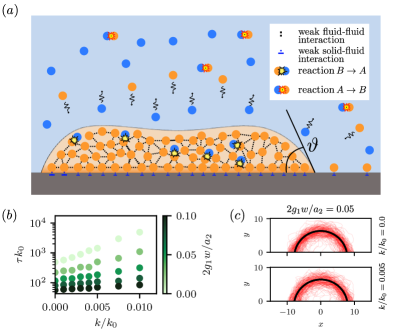
Figure 1: Driven reactions delay heterogeneous nucleation. (a) Schematic picture of a sessile reactive droplet. Droplet material is attracted to the wall and itself, leading to phase separation from solvent. In addition, active chemical reactions convert droplet material to solvent material inside the droplet, while the converse happens outside. This process leads to long-ranged diffusive fluxes, resulting in deformed macroscopic droplets. (b) Numerically determined nucleation times $\tau$ as a function of reaction rate $k$ for various wall affinities $g_{1}$. (c) Ensemble of critical nuclei for two reaction rates $k$ and positive wall affinity $g_{1}=0.025\,a_{2}/w$. (b-c) Simulations are detailed in the SI, section A; Model parameters are $\nu c_{0}=0.1$, $a_{2}/(\nu k_{B}T)=200$, $\nu=w^{2}$, $a_{4}=4a_{2}\nu$, and $k_{0}=\Lambda_{\mathrm{d}}a_{2}w^{-2}$.

Equilibrium states minimize the free energy $F$. As a necessary condition, the variation of $F$ with respect to $c$ must vanish, which yields the two conditions

$$f^{\prime}(c)-\kappa\nabla^{2}c =\mathrm{const}$$ (in the bulk) (3a)

$$\bm{n}\cdot\nabla c =\frac{g_{1}}{\kappa} \text{(at the boundary)}\;,$$ (3b)

where $\bm{n}$ denotes the outward normal of the surface $\partial V$. The first equation describes the balance of the exchange chemical potential $\mu=f^{\prime}(c)-\kappa\nabla^{2}c$, where the constant is determined from material conservation Weber et al. (2019). This generically yields a dense phase of concentration $c^{(0)}_{\mathrm{in}}\approx(2\nu)^{-1}+\sqrt{a_{2}/a_{4}}$ that is separated from a dilute phase of concentration $c^{(0)}_{\mathrm{out}}\approx(2\nu)^{-1}-\sqrt{a_{2}/a_{4}}$ by an interface of width $w=\sqrt{2\kappa/a_{2}}$. The dense phase typically assumes a spherical shape to minimize the surface tension $\gamma_{\mathrm{ds}}=2\sqrt{2\kappa a_{2}^{3}}/(3a_{4})$ between the two phases Weber et al. (2019). In contrast, Eq. (3b) describes a boundary condition, which determines the behavior of the system close to the wall. In particular, the droplet material is repelled from the wall if $g_{1}<0$ Gennes, Brochard-Wyart, and Quéré (2004). Since the droplet still maintains its spherical shape, its geometry at the wall is fully quantified by the contact angle $\vartheta$, which is given by the Young-Dupré equation, $\cos(\vartheta)=(\gamma_{\mathrm{ws}}-\gamma_{\mathrm{wd}})/\gamma_{\mathrm{ds}}$ Young (1805), where $\gamma_{\mathrm{ws}}$, $\gamma_{\mathrm{wd}}$, and $\gamma_{\mathrm{ds}}$ denote the surface tensions between wall-solvent, wall-droplet, and droplet-solvent, respectively. Since $g(c)$ directly quantifies surface energies, we have $\gamma_{\mathrm{wd}}\approx-g_{1}c^{(0)}_{\mathrm{in}}$ and $\gamma_{\mathrm{ws}}\approx-g_{1}c^{(0)}_{\mathrm{out}}$, resulting in

$$\cos(\vartheta)\approx\frac{3g_{1}}{a_{2}}\sqrt{\frac{a_{4}}{2\kappa}}\;.$$ (4)

This equation can only be solved for $\vartheta$ if the interactions between the droplet and the wall are weak, $|g_{1}|<g_{*}$ with $g_{*}\approx\sqrt{(2a_{2}^{2}\kappa)/(9a_{4})}$. In contrast, the droplet will be repelled from the wall if $g_{1}<-g_{*}$, and it will fully wet the wall if $g_{1}>g_{*}$. Since the interesting process of heterogeneous nucleation is related to partial wetting where $\vartheta$ is defined, we concentrate on the case $|g_{1}|<g_{*}$. In particular, we consider the case $g_{1}>0$, corresponding to an attractive wall that is the most probable site for nucleation.

To describe nucleation, we next specify the dynamics of the system. We start with the continuity equation

$$\partial_{t}c+\nabla\cdot\bm{j}=s\;,$$ (5)

where $\bm{j}$ denotes the diffusive exchange flux between droplet material and the solvent, and the source term $s$ describes chemical transitions Weber et al. (2019). The passive diffusive flux $\bm{j}$ is driven by gradients of the exchange chemical potential, $\bm{j}=-\Lambda_{\mathrm{d}}\nabla\mu+\bm{\eta}$, where $\Lambda_{\mathrm{d}}$ is the diffusive mobility and $\bm{\eta}$ denotes diffusive thermal noise, which obeys $\langle\eta_{i}(\bm{r},t)\rangle=0$ and the fluctuation dissipation theorem $\langle\eta_{i}(\bm{r},t)\eta_{j}(\bm{r}^{\prime},t^{\prime})\rangle=2k_{\mathrm{B}}T\Lambda_{\mathrm{d}}\delta_{ij}\delta\left(\bm{r}-\bm{r}^{\prime}\right)\delta\left(t-t^{\prime}\right)$, where $k_{\mathrm{B}}T$ is the thermal energy Jülicher, Grill, and Salbreux (2018); De Groot and Mazur (1984); God (1991). The system becomes active when we drive the reactions described by $s$ out of equilibrium Kirschbaum and Zwicker (2021). We focus on driven reactions that result in size-controlled droplets, which requires production of droplet material outside the droplet, while it is degrade inside Kirschbaum and Zwicker (2021); Weber et al. (2019). This behavior can be captured by the linear expression

$$s(c)=-k(c-c_{0})\;,$$ (6)

where $k$ sets the reaction rate and $c_{0}$ denotes the stationary state of the reaction scheme. We have shown previously that this case faithfully describes homogeneous nucleation in active systems and that the thermal noise associated with the reactions can be neglected since the diffusive noise $\bm{\eta}$ dominates on the length scales relevant for nucleation Ziethen, Kirschbaum, and Zwicker (2023). Taken together, our system is described by the stochastic partial differential equation

$$\partial_{t}c=\Lambda_{\mathrm{d}}\nabla^{2}\mu-k(c-c_{0})+\nabla\cdot\bm{\eta}\;,$$ (7)

augmented by the no-flux boundary condition $\bm{n}\cdot\bm{j}=0$, and Eq. (3b) describing local equilibrium at the boundary.

III Chemical reactions suppress heterogeneous nucleation

III.1 Numerical simulations reveal increased nucleation times

To investigate heterogeneous nucleation, we performed numerical simulations of Eq. (7) in a two-dimensional system. Here, we used finite differences to approximate derivatives and an Euler-Maruyama scheme to perform the time stepping Zwicker (2020). We applied periodic boundary conditions along the $x$-direction and Eq. (3b) on both boundaries in the $y$-directions. Repeating the simulations many times, we observed that the time $t_{\mathrm{nucl}}$, quantifying when the first droplet nucleates, follows an exponential distribution; see Supplementary Fig. 9. We thus define the nucleation time $\tau$ as the ensemble average of $t_{\mathrm{nucl}}$. Fig. 1b shows that $\tau$ decreases for stronger droplet-wall attraction (larger $g_{1}$), as expected for nucleation of passive droplets Kalikmanov (2013). In contrast, larger reaction rates $k$ lead to longer nucleation times $\tau$, indicating that active chemical reactions hinder nucleation, consistent with the results for homogeneous nucleation Ziethen, Kirschbaum, and Zwicker (2023). These numerical simulations indicate that repulsive walls (small $g_{1}$) and larger reactions (larger $k$) suppress heterogeneous nucleation, but they do not reveal the underlying principles governing the nucleation process.

III.2 Equilibrium surrogate model reveals trade-off between wall affinity and chemical reactions

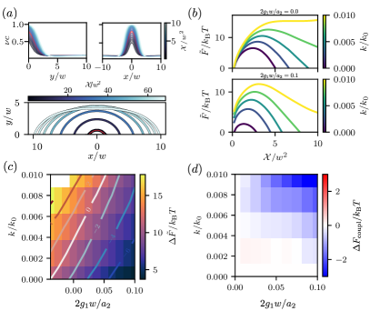
Figure 2: Reactions raise energy barrier of nucleation. (a) Cuts through concentration profile $c(x,y)$ along the two axes (top) and shape of droplet interface (bottom) along the nucleation path (colors) for $k/k_{0}=0.01$ and $g_{1}w/a_{2}=0.05$. The shape of the critical nucleus is indicated in red. (b) Energy $\tilde{F}$ of the surrogate model as a function of the nucleation coordinate $\mathcal{X}$ for various reaction rates $k$ for a neutral wall ($g_{1}=0$) and an attractive wall ($g_{1}=0.05\,a_{2}/w$). (c) Energy barrier $\Delta\tilde{F}$ as a function of $g_{1}$ and $k$. (d) Energy $F_{\mathrm{coupl}}$ following from Eq. 10 as a function of $g_{1}$ and $k$. (a-d) Model parameters are as in Fig. 1.

To understand the nucleation path in detail, we next map the active system onto a surrogate equilibrium system with long-ranged interactions, which is possible for the special case of the linear reactions that we consider. Briefly, we can re-write the dynamics given by Eq. (7) as $\partial_{t}c=\Lambda_{\mathrm{d}}\nabla^{2}\delta\tilde{F}[c]/\delta c+\nabla\cdot\bm{\eta}$ when we use the augmented free energy functional

$$\tilde{F}[c]=F[c]+F_{\mathrm{react}}[c]\;,$$ (8)

where

$$F_{\mathrm{react}}[c] =\frac{k}{2\Lambda_{\mathrm{d}}}\int\bigl{[}c(\bm{r})-c_{0}\bigr{]}\Psi(\bm{r})\,\mathrm{d}\bm{r}$$ (9)

captures the energy associated with reactions Liu and Goldenfeld (1989); Christensen, Elder, and Fogedby (1996); Muratov (2002). Here, $\Psi$ is the solution to the Poisson equation $\nabla^{2}\Psi=c_{0}-c(\bm{r})$ and describes the long-ranged interactions, which originate from the interplay of chemical reactions and diffusion in the original model. Since the surrogate model requires mass conservation, we solve for $\Psi$ employing Neumann boundary conditions, $\bm{n}.\nabla\Psi=0$.

We used the free energy of the surrogate model, given by Eq. (8), to map out the minimal energy path connecting the homogeneous state with the state where a droplet wets the wall. To do this, we used constrained optimization to obtain concentration profiles at successively larger values of a nucleation coordinate $\mathcal{X}$, which measures the amount of material inside the droplet; see SI, section B. Fig. 2a shows an example of such a minimal energy path, indicating that the maximal concentration inside the droplet increases alongside its size.

The minimal energy path allows us to evaluate the critical energy and the critical nucleus, which is the transition state of the nucleation process. Fig. 2b shows that chemical reactions generally increase $\tilde{F}$, potentially explaining why reactions suppress nucleation. However, reactions also increase $\tilde{F}$ of the homogeneous state when the wall is attractive ($g_{1}>0$). This is because the boundary condition given by Eq. (3b) perturbs the homogeneous state in a layer with a thickness of roughly the interfacial width $w$, leading to local reactive fluxes. To see how chemical reactions affect nucleation, we thus evaluated the energy difference $\Delta\tilde{F}$ between the transition state and the homogeneous initial state. Fig. 2c shows that $\Delta\tilde{F}$ increases with the reaction rate $k$, while it decreases with more attractive walls (larger $g_{1}$), which is expected Ziethen, Kirschbaum, and Zwicker (2023); Kalikmanov (2013).

We next quantified how chemical reactions interact with the wall affinity by decomposing the free energy barrier,

$$\Delta\tilde{F}(g_{1},k)=\Delta F_{\mathrm{pas}}(g_{1})+\Delta F_{\mathrm{react}}(k)+\Delta F_{\mathrm{coupl}}(g_{1},k)\;,$$ (10)

where $\Delta F_{\mathrm{pas}}=\Delta\tilde{F}(g_{1},k=0)$ quantifies the barrier for passive heterogeneous nucleation, $\Delta F_{\mathrm{react}}=\Delta\tilde{F}(g_{1}=0,k)$ is the energy barrier of chemically driven droplets at a neutral wall, and $\Delta F_{\mathrm{coupl}}(g_{1},k)$ denotes the energy due to the interaction of the two effects. Since we directly determined $\Delta\tilde{F}(g_{1},k)$, $\Delta F_{\mathrm{pas}}(g_{1})$, and $\Delta F_{\mathrm{react}}(k)$, we can infer $\Delta F_{\mathrm{coupl}}(g_{1},k)$ from Eq. (10). The data shown in Fig. 2d indicates a significant negative coupling between the wall affinity and the reactions, i.e., strong affinity to the wall can decrease the relative effect of chemical reactions.

The coupling between the wall affinity $g_{1}$ and the reaction rate $k$ is also apparent in the contour lines of equal $\Delta\tilde{F}$, where reactions and wall affinity compensate each other; see Fig. 2c. We show in the SI, section D that concave contour lines would be expected without coupling ($\Delta F_{\mathrm{coupl}}=0$), so that the slight convex shape of the observed lines is a strong indication for coupling. To analyze these contour lines in more detail, we approximate the coupling by a bilinear function, $\Delta F_{\mathrm{coupl}}(g_{1},k)=hg_{1}k$ with pre-factor $h$, motivated by Fig. 2d. Moreover, we use a linear approximation for the reactive energy Ziethen, Kirschbaum, and Zwicker (2023), $\Delta F_{\mathrm{react}}=mk$, and we express the energy associated with the passive case as Kalikmanov (2013)

$$\Delta F_{\mathrm{pas}}(g_{1}) =\frac{\gamma_{\mathrm{ds}}^{2}}{\Delta f}\bigl{[}2\vartheta(g_{1})-\sin(2\vartheta(g_{1}))\bigr{]}\;,$$ (11)

where $\Delta f=f(c_{0})-f(c_{\mathrm{in}}^{\mathrm{eq}})+f^{\prime}(c_{0})(c_{\mathrm{in}}^{\mathrm{eq}}-c_{0})$ and $\vartheta$ is given by Eq. (4). Taken together, the contour line associated with energy $\Delta F_{\mathrm{c}}$ then satisfies

$$k=\frac{1}{m+hg_{1}}\left[\Delta F_{\mathrm{c}}-\Delta F_{\mathrm{pas}}(g_{1})\right]\;.$$ (12)

We show in the SI, section D that the curvature of these contour lines is typically negative ($\partial^{2}k/\partial g_{1}^{2}>0$), consistent with the observed convex shape.

To explore the observed coupling further, we next ask how the energy $F_{\mathrm{react}}$, defined by Eq. (9), changes with the wall affinity $g_{1}$. We thus initialized droplets of fixed volume for various affinities $g_{1}$ and numerically calculated $F_{\mathrm{react}}$ inside the droplet; see SI, section D.4. Supplementary Fig. 11 shows that $F_{\mathrm{react}}$ indeed decreases with larger $g_{1}$, consistent with the negative effect we found above. However, this analysis only probes how different contact angles affect the reactions, whereas the reactions potentially also change the entire droplet shape away from a spherical cap.

IV Sessile active droplets spread along walls

IV.1 Droplets deviate from spherical cap shape after nucleation

The minimal energy paths that we obtained from the surrogate model not only provide energy barriers for nucleation but also the most likely droplet shape along the nucleation path. Fig. 2a shows that small droplets are shaped like a spherical cap, which corroborates the sampled critical droplet shapes shown in Fig. 1c. However, Fig. 2a also shows that larger droplets can deviate significantly from this equilibrium shape.

The droplet shape originates from a minimization of the free energy $\tilde{F}$ of the surrogate equilibrium model. If reactions are absent, surface tension $\gamma_{\mathrm{ds}}$ minimizes the interface between droplet and solvent material, resulting in a spherical shape with constant mean curvature. At the systems boundary, the shape must be compatible with the contact angle $\vartheta$ controlled by the energy balance that led to Eq. (4), which implies that attractive walls result in flatter spherical caps. The situation is more complicated with chemical reactions. The long-ranged interaction described by Eq. (9) leads to a repulsion of the droplet material, analogously to electrostatic repulsion of charged material. Consequently, different parts of the droplet repel each other Rayleigh (1882), which can induce spontaneous splitting for large bulk droplets Golestanian (2017); Zwicker et al. (2017) and explains why active droplets spread along the wall.

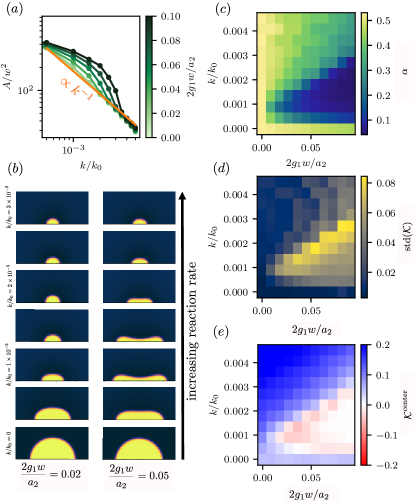
Figure 3: Active droplets spread along walls. (a) Droplet area as a function of the reaction rate $k$ for different wall affinities $g_{1}$. (b) Concentration fields of sessile droplets for two values of $g_{1}$ and various $k$. (c) Aspect ratio $\alpha$ of sessile droplet as a function of $g_{1}$ and $k$. (d) Standard deviation of the interface curvature $\mathcal{K}$ as a function of $g_{1}$ and $k$. (e) $\mathcal{K}$ evaluated at the droplet center as a function of $g_{1}$ and $k$. (a–e) Model parameters given in Fig. 1.

IV.2 Interplay of reactions and wall affinity can deform macroscopic droplets

To understand how the interplay between wall affinity and driven chemical reaction influences the droplet shape, we next study the stationary shapes of sessile droplets numerically. We initialized droplets at the wall and simulated their time evolution for different reaction rates $k$ and wall affinities $g_{1}$ until steady states were reached. To get an initial understanding, we first quantified droplet size, which is an area in our two-dimensional simulations. If droplet size is controlled by the reaction-diffusion length scale $L=(D/k)^{1/2}$, with some diffusivity $D$, we expect the droplet size to scale with $k^{-1}$. Fig. 3a indeed reveals such a scaling, at least for large reaction rates. In contrast, for intermediate rates, we observe significant deviations, which increase with the wall affinity. The snapshots shown in Fig. 3b suggest that intermediate reaction rates $k$ lead to strongly deformed droplets, which could explain the observed size-dependence.

We next quantified droplet shapes by analyzing the curve describing the interface, defined as the iso-contour $c=0.5$. First, we determined the aspect ratio $\alpha$, which is defined as the quotient of the lengths of the minor and major axis (see Fig. 3c). Second, we quantified the curvature $\mathcal{K}$ of the interface (see SI, section C) and determined its variation along the interface (see Fig. 3d) as well as the curvature at the center point (see Fig. 3e). All three quantifications shown reveal the same fundamental dependence: Droplets are essentially spherical caps when reactions are absent ($k=0$), consistent with expectations Gennes, Brochard-Wyart, and Quéré (2004). Moreover, droplets are spherical for neutral walls ($g_{1}=0$), even when reactions are strong, because all fields are radially symmetric in this symmetric case. Interestingly, droplets also exhibit a spherical cap shape for large reaction rates, likely because strong reactions reduce droplet size so interfacial effects dominate. Between these extreme values, we observe strong deviations from a spherical shape, both in the snapshots (Fig. 3b) and in the quantifications (Fig. 3c–e). In fact, for a given wall attraction $g_{1}$, we empirically find an intermediate rate $k$ for which the deformations are maximally, and this rate increases with $g_{1}$. Taken together, these quantifications reveal an interplay between wall attraction and reactions, which leads to macroscopic deformations of sessile droplets.

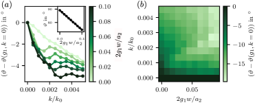
Figure 4: Reactions affect contact angles. (a, b) Deviation of contact angle $\vartheta$ from passive case ($k=0$) as a function of reaction rate $k$ for various wall affinities $g_{1}$. The inset shows $\vartheta$ as a function of $g_{1}$ for $k=0$. Model parameters given in Fig. 1.

The macroscopic deformations induced by the reactions affect the entire interface and could thus also impact the contact angle $\vartheta$. To test this, we evaluated the slope $-\partial_{x}c/\partial_{y}c$ along the implicit curve $c(x_{I},y_{I})=0.5$ and measured the associated $\vartheta$ at the boundary. The inset in Fig. 4a shows that $\vartheta$ decreases with increasing wall affinity $g_{1}$, consistent with the prediction from Eq. (4). However, the data in Fig. 4a also indicates that $\vartheta$ decreases for larger reaction rates $k$, indicating an effect of the reactions. For attractive walls ($g_{1}>0$), the contact angle first declines sharply for increasing $k$, although this decline becomes weaker for larger $k$ and there is even a brief non-monotonic behavior. The value of $k$, where this non-monotonic behavior is observed, depends on $g_{1}$ and coincides with the maximal shape deformation of the droplets (compare Fig. 4b to Fig. 3a). Chemically active sessile droplets thus exhibit changes in apparent contact angle concomitantly with global shape deformations.

IV.3 Anisotropic fluxes cause droplet deformation

To gain further insights into shape deformations, we next analyze how reactions disturb the spherical cap shapes expected for passive droplets. We consider a spherical cap described by a radius $R$ and contact angle $\vartheta$ in the half-space $y>0$. To describe the droplet shape explicitly, we use an effective droplet model Weber et al. (2019), assuming a thin interface ($w\ll R$), so we can approximate the dynamics of the concentration fields $c_{i}$ by reaction-diffusion equations

$$\partial_{t}c_{i}\approx D\nabla^{2}c_{i}-k(c_{i}-c_{0})\;,$$ (13)

inside ($i=\mathrm{in}$) and outside ($i=\mathrm{out}$) the droplet; see SI, section E. Here, we linearized Eq. (7) without noise around the concentrations $c^{(0)}_{\mathrm{in}}$ and $c^{(0)}_{\mathrm{out}}$, so the diffusivity is given by $D=\Lambda_{\mathrm{d}}f^{\prime}{{}^{\prime}}(c^{(0)}_{\mathrm{in}})=\Lambda_{\mathrm{d}}f^{\prime}{{}^{\prime}}(c^{(0)}_{\mathrm{out}})$ for our choice of a symmetric free energy Weber et al. (2019). To solve the reaction-diffusion problem, we employ polar coordinates $(r,\varphi)$ centered at the sphere describing the spherical cap. We impose $\partial_{y}c_{i}|_{y=0}=0$ and $\partial_{r}c_{\mathrm{out}}|_{r\rightarrow\infty}=0$ at the system boundary. The conditions at the droplet interface are governed by the local phase equilibrium and read $c_{i}(R)=c_{i}^{(0)}+\beta_{i}\gamma_{\mathrm{ds}}/R$, where $\beta_{i}=2/[(c_{\mathrm{in}}^{(0)}-c_{\mathrm{out}}^{(0)})f^{\prime\prime}(c_{i}^{(0)})]$ quantifies surface tension effects for $i=\mathrm{in},\mathrm{out}$ Weber et al. (2019). For simplicity, we consider the quasi-stationary situation where the concentration fields equilibrate faster than the interfacial shape. The resulting stationary state solutions to Eq. (13) then depend on the reaction-diffusion length scale $L=\sqrt{D/k}$, the average concentration $c_{0}$, and the boundary conditions. The general solution of this Helmholz equation reads

$$c_{i}(r,{\varphi})=c_{0}\\ +\sum_{n=0}^{\infty}\!\left[A_{n}^{i}I_{\lambda_{n}}\!\!\left(\frac{r}{L}\right)+B_{n}^{i}K_{\lambda_{n}}\!\!\left(\frac{r}{L}\right)\right]\!\cos(\lambda_{n}\bigl{(}{\varphi}-\vartheta)\bigr{)}\;,$$ (14)

where $I_{\lambda_{n}}(z)$ and $K_{\lambda_{n}}(z)$ are the modified Bessel functions of first and second kind. Here, the wavelength $\lambda_{n}=n\pi/\vartheta$ of the polar coordinate is quantized by the boundary conditions, which can also be used to determine the series coefficients $A_{n}^{i}$ and $B_{n}^{i}$ as described in the SI, section E. Taken together, this approach provides approximate solutions for the concentration profiles inside and outside the droplet.

The concentration fields imply fluxes $\bm{j}_{i}=-D\nabla c_{i}$, which can affect droplet shapes. Indeed, the interface speed ${v}_{\mathrm{n}}$ normal to the interface reads Weber et al. (2019)

$${v}_{\mathrm{n}}(\varphi)=\frac{\bm{j}_{\mathrm{in}}(r=R,\varphi)-\bm{j}_{\mathrm{out}}(r=R,\varphi)}{c_{\mathrm{in}}^{(0)}-c_{\mathrm{out}}^{(0)}}\cdot\bm{n}\;,$$ (15)

where $\bm{n}$ is the normal vector of the interface. Using Eq. (14), we find

$${v}_{\mathrm{n}}=\frac{1}{c_{\mathrm{in}}^{(0)}-c_{\mathrm{out}}^{(0)}}\sum_{n=0}^{\infty}\mathcal{C}_{n}(R,L,\vartheta)\cos\left(\lambda_{n}{\varphi}\right)\;,$$ (16)

with

$$\mathcal{C}_{n}(R,L,\vartheta)=\left(D_{\text{out }}A_{n}^{\text{out }}-D_{\text{in }}A_{n}^{\text{in }}\right)I_{\lambda_{n}}^{\prime}\left(\frac{R}{L}\right)\\ +\left(D_{\text{out }}B_{n}^{\text{out }}-D_{\text{in }}B_{n}^{\text{in }}\right)K_{\lambda_{n}}^{\prime}\left(\frac{R}{L}\right).$$ (17)

This interfacial speed ${v}_{\mathrm{n}}$ quantifies how chemical reactions would disturb the spherical cap shape.

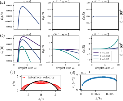
Figure 5: Reactions cause non-isotropic interface speeds. (a) Series coefficients $\mathcal{C}_{n}$ as a function of droplet size $R$ for $n=0,1,2$ at a neutral wall ($g_{1}=0$, contact angle $\vartheta=90^{\circ}$) for $k=0.0025$. (b) $\mathcal{C}_{n}$ as a function of $R$ for an attractive wall ($\vartheta=60^{\circ}$). (c) Interface velocity $v_{\mathrm{n}}\bm{n}$ (red arrows) predicted from Eq. (16) using the first three modes for a spherical cap of $R/w=7$ for $\vartheta=60^{\circ}$ (black line). (d) $|\mathcal{C}_{1}|$ as a function of the reaction rate $k$ for $\vartheta=60^{\circ}$. (a–d) Additional parameters are derived from values given in Fig. 1.

We start by examining the shape of a droplet on a neutral wall ($g_{1}=0$). Fig. 5a shows that only the $n=0$ mode contributes, whereas $A^{i}_{n}=B^{i}_{n}=0$ for $n\geq 1$, consistent with the observed spherical shapes. The zeroth mode is essentially unchanged for an attractive wall ($g_{1}>0$, $\vartheta<\pi/2$, Fig. 5b), but the first and second modes become important for larger droplet sizes, indicating non-spherical droplet shapes. The dependence of these modes on the droplet radius $R$ captures the behavior we observed so far: For very small radii, the zeroth mode is negative, indicating an unstable size. Consequently, droplets can only grow spontaneously when $R$ exceed the first root of $\mathcal{C}_{0}(R)$, which thus corresponds to the size of the critical nucleus. At the critical size, the higher modes shown in the right two panels in Fig. 5b are vanishingly small, consistent with the spherical shape of critical nuclei observed in Fig. 1c. Droplets larger than the critical size grow until they reach a stationary state, marked by the second root of $\mathcal{C}_{0}(R)$ in Fig. 5b; see also ref. Zwicker, Hyman, and Jülicher (2015). At this stationary state, the zeroth mode does not contribute to the dynamics, but higher-order modes, which are connected to shape deformations, do. Indeed, Fig. 5c shows that the interface speed of a stationary droplet with radius $R^{*}$, chosen such that $\mathcal{C}_{0}(R^{*})=0$, is such that the droplet flattens and spreads along the walls. Taken together, the analysis of the first mode of a droplet with a stationary size indicates that fluxes caused by the driven reactions deform the droplet.

To understand droplet deformations in detail, we next focus on the first mode ($n=1$). Fig. 5d shows that its magnitude $|\mathcal{C}_{1}(R=R^{*},k)|$ vanishes when reaction are absent ($k=0$), consistent with the expected spherical cap shape of passive droplets. Larger reaction rates $k$ first cause $|\mathcal{C}_{1}|$ to increase, but $|\mathcal{C}_{1}|$ then decreases beyond a critical value of $k$. This non-monotonic behavior is qualitatively consistent with the shape deformations shown in Fig. 3 and might be related to the steady state size of reactive droplets: Higher reaction rates $k$ reduce the droplet size (see Fig. 3a and ref. Zwicker, Hyman, and Jülicher (2015)), leading to smaller magnitudes of the droplet deforming modes; see Fig. 5b. In summary, chemical reactions combined with symmetry breaking by an attractive wall lead to non-isotropic flows that cause droplet deformation.

IV.4 Reactions deform sessile 3D droplets

So far, we analyzed deformed droplets only in two spatial dimensions. To check whether the observed effects persist in three dimensions, we performed a simulation for the parameter regime where droplets are deformed. Supplementary Fig. 13 shows that such droplets are circular in the $xy$-plane and are deformed only in the $z$-direction. Consequently, simulations using cylindrical symmetry are suitable to describe the problem. Fig. 6 shows that we find spherical cap shapes for small and large reaction rates $k$, and strongly deformed droplets between these extremes, consistent with our results for attractive walls in two-dimensional systems. Taken together, we thus expect that our results translate directly to three-dimensional systems.

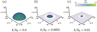
Figure 6: Reactions deform sessile 3D droplets. Concentration profiles $c(x,y,z)$ of 3D droplets in stationary state for various reaction rates $k$ at an attractive wall ($g_{1}=0.05\,a_{2}/w$). Simulations were performed in cylindrical symmetry using the parameters $r_{\mathrm{max}}/w=64$, $dr/w=1$, $z_{\mathrm{max}}/w=32$, $dz/w=0.25$. Additional parameters can be found in Fig. 1.

V Electrostatic analogy explains effects of driven reactions

So far, we have focused on simulating the dynamical equation (7) and analyzed the simplified reaction-diffusion equation (13). In this final section, we now investigate the equilibrium surrogate model given by Eq. (8) in detail, which will allow us to interpret the reactions as long-ranged electrostatic interactions.

The energy $F_{\mathrm{react}}$ associated with reactions, given by Eq. (9), reveals that the deviation of the concentration field $c(\bm{r})$ from the reaction equilibrium $c_{0}$ can be interpreted as a charge density. This interpretation only works for the linearized reactions given by Eq. (6) and when the average concentration field is equal to $c_{0}$, e.g., when $\int c\,\mathrm{d}V=c_{0}V$, which implies a charge neutral system in the electrostatic interpretation. Fig. 7(a) shows a typical concentration profile of a sessile droplet, indicating that the droplet can be interpreted as a positively charged ball surrounded by a cloud of negative charges, so that the entire system is charge neutral. The reaction-diffusion length scale $L=\sqrt{D/k}$ controls the extent of the cloud and the reaction rate $k$ determines the magnitude of the electrostatic interaction. Even though the sessile droplet in Fig. 7(a) looks as if it would form a dipole with the surrounding negative charges, this is not the case since image charges restore the symmetry. Distant droplets thus hardly interact with each other.

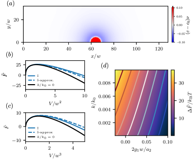
Figure 7: Electrostatic analogy explains nucleation behavior. (a) Effective charge density $c(\bm{r})-c_{0}$ of a sessile droplet for reaction rate $k/k_{0}=0.005$. (b, c) Energy barrier $\tilde{F}$ as a function of the volume $V$ in 2D (panel b, $k/k_{0}=0.001$) and 3D (panel c, $k/k_{0}=0.01$) for various approximations: The full theory (solid blue lines, see Eq. (82) and Eq. (96)) is compared to the approximations given in Eqs. (18) (dashed lines) and the expression for $k=0$ (black lines). The contact angle is $\vartheta=80^{\circ}$. (d) Nucleation barrier $\Delta\tilde{F}$ determined from maximizing $\tilde{F}(V)$ given by Eq. (18a) for various $k$ and $g_{1}$. (a–d) Additional parameters are given in Fig. 1.

To be more quantitative, we next calculate the total energy of a single sessile droplet in the limit of a thin interface, also known as a capillary approximation; see SI, section G. The approximate expressions for small droplets in two and three dimensions read Ziethen, Kirschbaum, and Zwicker (2023); Muratov (2002)

$$\tilde{F}_{\mathrm{2D}} \approx\bigl{[}0.029+0.32\log(LV_{\mathrm{2D}}^{-\frac{1}{2}})\bigr{]}\frac{(c_{\mathrm{in}}^{(0)}-c_{0})^{2}}{\Lambda_{\mathrm{d}}}kV_{\mathrm{2D}}^{2}$$

$$\quad-\Delta fV_{\mathrm{2D}}+\gamma_{\mathrm{ds}}A_{\mathrm{2D}}\;,$$ (18a)

$$\tilde{F}_{\mathrm{3D}} \approx 0.039\frac{(c_{\mathrm{in}}^{(0)}-c_{0})^{2}}{\Lambda_{\mathrm{d}}}kV_{\mathrm{3D}}^{\frac{5}{3}}-\Delta fV_{\mathrm{3D}}+\gamma_{\mathrm{ds}}A_{\mathrm{3D}}\;,$$ (18b)

where the bulk energy proportional to $\Delta f=f(c_{0})-f(c_{\mathrm{in}})+f^{\prime}(c_{0})(c_{\mathrm{in}}-c_{0})$ scales with the droplet volume $V$, whereas the surface energy proportional to $\gamma_{\mathrm{ds}}$ scales with the effective size of the interface, which depends on the contact angle $\vartheta$: $A_{\mathrm{2D}}=\sqrt{2V_{\mathrm{2D}}(2\vartheta-\sin(2\vartheta))}$ and $A_{\mathrm{3D}}=4\pi(3V_{\mathrm{3D}}/[\pi(2+\cos(\vartheta))(1-\cos(\frac{\vartheta}{2})^{2})])^{\frac{2}{3}}\sin(\frac{\vartheta}{2})^{4}$. For simplicity, we neglect the influence of $\vartheta$ on the electrostatic energies associated with the charge distribution given by the respective first terms proportional to $k$. Instead, we use the expression for one half of a spherical droplet on a wall as an approximation; see SI, section G. Neglecting logarithmic corrections, we thus find that reactive energies scale as $R^{2+d}$, bulk energies as $R^{d}$, and surface energies as $R^{d-1}$, when droplets are small and $d$ is the space dimension.

We first use the approximate energies to investigate nucleation. The surface energy dominates for small droplets, explaining why nucleated droplets close to the critical size are spherical; see Fig. 1c. Eqs. (18) also show that chemical reactions raise the nucleation barrier (see Fig. 7(b,c)), consistent with suppressed nucleation. The associated energy barrier $\Delta\tilde{F}$ shown in Fig. 7d exhibits a very similar dependence on the reaction rate $k$ and the wall affinity $g_{1}$ compared to the numerically determined barriers shown in Fig. 2c. However, since we do not consider the contact angle $\vartheta$ in the simplified electrostatic energy given in Eq. (18), this approximation cannot capture the coupling between $k$ and $g_{1}$ we revealed above. Moreover, the capillary approximation used here is known to overestimates the energy barrier for droplet formation Kalikmanov (2013) since it assumes a well-defined separation of the droplet and the surrounding dilute phase during nucleation. Yet, we can conclude that the electrostatics do not affect the shape of small droplets, but they oppose their formation, thus lowering nucleation rates.

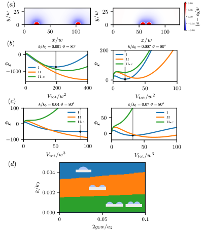
Figure 8: Electrostatic analogy explains droplet deformations. (a) Effective charge density $c(\bm{r})-c_{0}$ of two sessile droplet that are well-separated (left) or directly adjacent (right) for for a reaction rate $k/k_{0}=0.005$. (b, c) Energy barrier $\tilde{F}$ as a function of the total volume $V_{\mathrm{tot}}$ of one droplet (I, blue lines) and two droplets that are well-separated (II, orange lines) or adjacent (II-c, green lines) in 2D (b) and 3D (c) determined using the full theory; see  SI, section G. Parameters are indicated in the panels. (d) State diagram indicating which state has the lowest energy $\tilde{F}$ at the total volume where a single droplet is stable as a function of reaction rate $k$ and wall affinity $g_{1}$. The single droplet has the lowest energy in the blue region and for $k=0$, whereas the separated droplets have lower energy in the orange region, and both connected and separated droplets have lower energies in the green region. (a–d) Additional parameters are given in Fig. 1.

To discuss shape deformations and splitting of droplets, we next approximate these two situations by considering two sessile droplets with total volume $V_{\mathrm{tot}}$ that either touch each other or are well-separated; see Fig. 8a. If $\tilde{F}(V_{\mathrm{tot}})$ denotes the energy of the single droplet of volume $V_{\mathrm{tot}}$, the two well-separated droplets have a total energy of $2\tilde{F}(\frac{1}{2}V_{\mathrm{tot}})$. In addition, the two connected droplets exhibit an electrostatic repulsion, which we approximate as the repulsion between two point charges; see SI, section G. Since the approximations given in Eqs. (18) only hold for small droplets, we here obtain $\tilde{F}(V)$ from Eq. (82) and Eq. (96) in the Supplement. Taken together, we can thus compare the energies of the two droplets at different separation to the energy of a single droplet in 2D and 3D for various $V_{\mathrm{tot}}$; see Fig. 8(b,c). Without reactions ($k=0$), the energy of two droplets is always higher than that of a single droplet, consistent with a minimization of surface energies and absent droplet deformations. Moreover, $\tilde{F}(V)$ decreases monotonously beyond the critical size, implying that droplets grow until they are limited by system size. The picture changes qualitatively when reactions are enabled (and droplets become charged in the electrostatic picture): Even for arbitrarily small $k$, $\tilde{F}(V)$ develops a minimum at a finite size $V$ and the electrostatic energy makes larger droplets unfavorable; see Fig. 8(b,c). Since the minimal energy is negative (implying that the droplet is favored over the homogeneous state), we observe that the states with two droplets (orange curves) have lower minima than the one-droplet states (blue curves), which implies that a large system would prefer to have many droplets. A large droplet count could emerge either from nucleating additional droplets or from splitting existing droplets.

To investigate droplet splitting, we compare the minimal energy of a single droplet with the energy of the two-droplet states at the corresponding total volume $V_{\mathrm{tot}}$. Fig. 8b shows that the two-droplet states can have lower energy for small reaction rates $k$, suggesting that a droplet with this volume might deform spontaneously. In contrast, the right panel shows that a single droplet has lower energy for large reaction rates $k$, suggesting that the single droplet is stable. The transition between these cases marks the onset of droplet deformation, which depends on the reaction rate $k$ and the wall affinity $g_{1}$. Fig. 8d suggests that droplets deform if reactions are not too strong and larger $g_{1}$ favor deformations; similar to Fig. 3(c-e). However, in contrast to Fig. 3(c-e), the simple scaling theory predicts that the deformed droplets (mimicked by the two adjacent droplets) are favored even when $g_{1}=0$. It is likely that deformations are kinetically suppressed, i.e., that small deformations are energetically unfavorable and we thus do not observe them.

The predicted transition from a single to a deformed and then split droplet can be understood as a competition between surface energies (favoring compact droplets) and effective electrostatic repulsion (favoring elongated droplets) in conjunction with the favored finite droplet size due to reactions. Droplets are spherical at large reaction rates $k$ since large $k$ implies small droplets where surface energies dominate. Smaller reactions imply larger droplets, where the electrostatic effects are stronger and eventually favor deformed droplets that can also split. However, if reactions are absent, we again observe spherical droplets since there are no electrostatic effects.

In summary, interpreting the reactions using electrostatics explains the delayed nucleation and droplet deformation. Nucleation is suppressed since electrostatics disfavor an accumulation of charges, but the critical droplets are still spherical since surface energies dominate. In contrast, larger droplet can minimize the total energy by deforming, which enlarges the average distance between charges and thus lowers the electrostatic energy at the expense of a larger surface energy. In this case, the deformed droplets can also grow beyond the volume predicted for spherical shapes, consistent with Fig. 3a.

VI Discussion

We showed that nucleation is accelerated by attractive walls and suppressed by active chemical reactions, consistent with our previous results Ziethen, Kirschbaum, and Zwicker (2023). However, we also found an intricate interplay between the two processes, likely stemming from shape modifications in sessile droplets. While the shape of critical nuclei is in agreement with a spherical cap, consistent with passive scenarios Gennes, Brochard-Wyart, and Quéré (2004), we found massive deformations for larger droplets at intermediate reaction rates. Within the surrogate model, the elongated droplets can also be interpreted as a trade-off between surface tension and effective electrostatic repulsion, which demonstrates that the active chemical reactions mediate a repulsive long-ranged interaction.

Our study of sessile active droplets provides the first step toward understanding the interplay of chemically active droplets with other structures. For simplicity, we focused on a two-component mixture, whereas cells exhibit a staggering complexity involving thousands of different components, which could be described by a multicomponent extension of our theory Mao et al. (2018); Zwicker and Laan (2022). Furthermore, we considered reactions that depend linearly on composition, but realistic, thermodynamically consistent reactions are more complex Zwicker (2022). While our previous work suggests that linear reactions capture nucleation quantitatively Ziethen, Kirschbaum, and Zwicker (2023), the shape of macroscopic droplets might change drastically, e.g., when surface reactions are additionally taken into account Liese et al. (2023). Finally, we only studied flat walls, but boundaries in cells are typically curved and deformable Agudo-Canalejo et al. (2021); Kusumaatmaja et al. (2021). Incorporating these aspects will likely require more advanced computational methods (such as Mokbel et al. (2023)), but we expect the general behavior that we unveiled here to persist.

Active control of phase separation is a challenge in cells. Our work suggests that cells could use chemical reactions to fine-tune the rate of heterogeneous nucleation as well as the shape of sessile droplets. Such deformed droplets may offer better control of wall deformations by condensation, e.g., by using less material than a spherical cap to achieve the same deformation. Such a regulation process would be a fascinating example combining control via active chemistry and a membrane surface Snead and Gladfelter (2019). Moreover, our model serves as an intriguing example of boundary effects in active field theories, inviting comparisons with other active field theories Turci and Wilding (2021); Turci, Jack, and Wilding (2023).

Data Availability Statement

The data that support the findings of this study are available from the corresponding author upon reasonable request.

AUTHOR DECLARATIONS

Conflict of Interest

The author have no conflicts to disclose.

Author Contribution

N.Z. performed the numerical simulations, did the formal analysis, and wrote the first draft of the manuscript. All authors conceived the project, analyzed the data, and edited the manuscript.

Appendix A Direct sampling of nucleation times and critical droplet shapes

To extract the mean nucleation time, we used direct sampling of the nucleation events. To do so, Eq. 5 in the main text was solved using py-pde Zwicker (2020). The simulation was stopped when a droplet was detected, and the concentration field of the critical droplet was saved. We used the mean concentration inside the largest cluster as a nucleation coordinate. During nucleation this quantity shows a steep increase which marks the nucleation event. The nucleation time is not sensitive on the threshold of the order parameter since there is a clear time scale separation between the formation of a critical nucleus and the growth of the droplet. The statistics of the nucleation time was extracted over multiple simulations and the time scale of the exponential probability distribution (see Fig. 9) function was evaluated. To get the ensemble of critical nuclei, the contours of the critical droplets were extracted from the critical phase fields using a marching squares algorithm van der Walt et al. (2014).

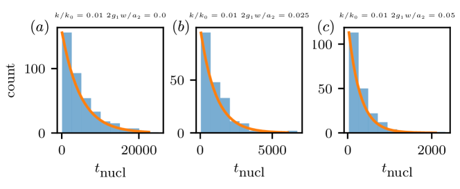
Figure 9: Distribution of nucleation times for different wall affinities $g_{1}$ and constant non-zero reaction rate $k_{0}$.

Appendix B Constrained optimizations to uncover minimal energy path

The minimal energy path comprises a sequence of concentration profiles that connects the homogeneous state to a stationary droplet. We determine the path using a reaction coordinate $\mathcal{X}$, which measures the mass concentrated in the nucleus,

$$\mathcal{X}[c]=\int\frac{1}{2}\left[1+\tanh\left(\Gamma c-\frac{\Gamma}{2\nu}\right)\right]\mathrm{d}V\;,$$ (19)

where $\Gamma=10$. We determine the minimal energy path by minimizing the free energy $\tilde{F}$ (given in Eq. 9 of the main text) with constrained values of $\mathcal{X}$. We impose a value $\mathcal{X}_{0}$ of the reaction coordinate using a Lagrange multiplier $\lambda$ and minimize

$$\hat{F}[c,\lambda]=\tilde{F}[c]-\lambda(\mathcal{X}[c]-\mathcal{X}_{0})$$ (20)

by evolving the partial differential equations

$$\partial_{t}c =\Lambda_{D}\nabla^{2}\frac{\delta\hat{F}}{\delta c}\;,$$ (21a)

$$\partial_{t}\lambda =-\Lambda_{L}\frac{\delta\hat{F}}{\delta\lambda}\;,$$ (21b)

which corresponds to conserved and non-conserved dynamics with mobilities $\Lambda_{D}$ and $\Lambda_{L}$, respectively. We use $\Lambda_{D}=1$ and $\Lambda_{L}=100$, which proved a good compromise between speed and stability. Using this procedure, the profiles $c(\bm{r})$ that minimize $\hat{F}$ for each value $\mathcal{X}_{0}$ of the constraint comprise the minimal free energy path. The profile with the largest energy $\tilde{F}$ corresponds to the saddle point and thus the critical nucleus.

Appendix C Curvature calculation

The curvature $\mathcal{K}$ and the slope $s$ of an implicit curve defined by $c(x_{I},y_{I})=0.5$ can be calculated as Goldman (2005)

$$\mathcal{K} =\frac{-(\partial_{y}c)^{2}\partial_{x}^{2}c+2\partial_{x}c\partial_{y}c\partial_{xy}c-(\partial_{x}c)^{2}\partial_{y}^{2}c}{((\partial_{x}c)^{2}+(\partial_{y}c)^{2})^{(3/2)}}\;,$$ (22)

$$s =-\frac{\partial_{x}c}{\partial_{y}c}\;,$$ (23)

evaluated at $\{x_{I},y_{I}\}$. Since the numerical fields are discrete, we use linear interpolation to evaluate the curvature and the slope on the interface line.

Appendix D Coupling of chemical reactions and wall affinities are crucial to explain the energy barriers

D.1 Passive energy barrier

The passive energy of a sessile droplet can be written as

$$F=-\Delta fV+\gamma_{\mathrm{ds}}A_{\mathrm{ds}}+\gamma_{\mathrm{wd}}A_{\mathrm{wd}}+\gamma_{\mathrm{ws}}(A_{\mathrm{w}}-A_{\mathrm{wd}})\;,$$ (24)

where $\Delta f=f(c_{0})-f(c_{\mathrm{in}}^{\mathrm{eq}})+\partial_{c}f(c_{0})(c_{\mathrm{in}}^{\mathrm{eq}}-c_{0})$, $A_{\mathrm{ds}}$ is the droplet solvent interface, $A_{\mathrm{wd}}$ is the wall droplet interface and $A_{\mathrm{w}}$ is the total area of the wall. Since $\gamma_{\mathrm{ds}}\cos(\vartheta)=\gamma_{\mathrm{ws}}-\gamma_{\mathrm{wd}}$, we can rewrite this expression as

$$F=-\Delta fV+\gamma_{\mathrm{ds}}\left(A_{\mathrm{ds}}-A_{\mathrm{wd}}\cos(\vartheta)\right)+\gamma_{\mathrm{ws}}A_{\mathrm{w}}\;.$$ (25)

The last term only gives a constant offset and will be dropped in the following. For a spherical cap geometry in two dimensions, we obtain

$$F=\left(\frac{1}{2}\Delta fR^{2}+\gamma_{\mathrm{ds}}R\right)(2\vartheta-\sin(2\vartheta))\;,$$ (26)

and a critical droplet radius of $R_{\mathrm{crit}}=\gamma_{\mathrm{ds}}/\Delta f$. The resulting energy barrier is then given by

$$\Delta F=\frac{\gamma_{\mathrm{ds}}}{2\Delta f}(2\vartheta-\sin(2\vartheta))\;.$$ (27)

The wetting angle $\vartheta$ can also be expressed as a function of our microscopic parameters, $\vartheta=\arccos\left(\frac{3g_{1}}{a_{2}}\sqrt{\frac{a_{4}}{2\kappa}}\right)$.

D.2 Augmented energy barrier by chemical reactions

The simplest assumption for how chemical reactions and wall affinities affect the energy barrier between homogeneous and droplet state is a simple superposition of the two. We consequently propose

$$\Delta F=\frac{\gamma_{\mathrm{ds}}^{2}}{2\Delta f}(2\vartheta-\sin(2\vartheta))+mk,$$ (28)

where we for simplicity assumed a linear relation for the reactive energy barrier, $\Delta F_{\mathrm{react.}}=mk$, in line with our previous results Ziethen, Kirschbaum, and Zwicker (2023). We now want to look at contour lines of the energy barrier (where chemical reactions and wall affinity compensate each other) and obtain

$$k_{\mathrm{contour}}=\frac{1}{m}\left[\mathrm{const}-\frac{\gamma^{2}}{\Delta f}\left(2\vartheta-\sin(2\vartheta)\right)\right]\;.$$ (29)

The second derivative is given by

$$\frac{\partial^{2}k_{\mathrm{contour}}}{\partial g_{1}^{2}}=-\frac{2d^{3}g_{1}\gamma_{\mathrm{ds}}^{2}}{\Delta f\sqrt{1-d^{2}g_{1}^{2}}}<0\;,$$ (30)

where $d=\frac{3}{a_{2}}\sqrt{\frac{a_{4}}{2\kappa}}$. Consequently, the contour lines are concave functions of $g_{1}$, whereas the contours in the data are slightly convex.

D.3 Additional coupling

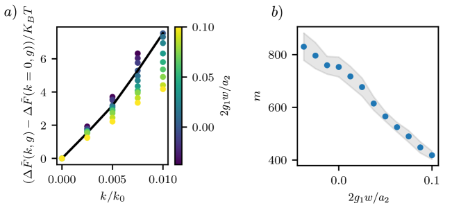
Figure 10: (a) Relative increase of the energy barrier $\Delta\tilde{F}$ with the reaction rate $k$ for different wall affinities $g_{1}$. (b) Fitted slope of the data in panel a as a function of the wall affinity $g_{1}$.

We measured the slope of the energy barrier $m$ for different values of $g_{1}$ and found a linear decrease (see Fig. 10). To capture this observation we add the lowest order coupling between reactions and wall affinities,

$$\Delta F=\Delta F_{\mathrm{wall}}(g_{1})+mk+hkg_{1}\;,$$ (31)

and we obtain for the contour line

$$k_{\mathrm{contour}}=\frac{1}{m+hg_{1}}\left[\mathrm{const}-\Delta F_{\mathrm{wall}}(g_{1})\right]\;.$$ (32)

The second derivative in the limit of small wall affinities is then given by

$$\frac{\partial^{2}k_{\mathrm{contour}}}{\partial g_{1}^{2}}=\frac{2((\mathrm{const}-\frac{\pi\gamma_{\mathrm{ds}}^{2}}{\Delta f})+\frac{\gamma_{\mathrm{ds}}^{2}}{\Delta f}dg_{1})h^{2}-\frac{8\gamma_{\mathrm{ds}}^{2}dh}{\Delta f}(g_{1}h+m)}{(g_{1}h+m)^{3}}\;,$$ (33)

which for typical parameters is positive and thus shows concave behavior in agreement with the data for $h<0$.

D.4 Effect of spherical cap shape on reactive energy

To test the effect of different contact angles $\vartheta$ on the reactive energy, we initialized droplets for different wall affinities $g_{1}$. We then evaluated the reactive energy by integrating Eq. 9, neglecting the contribution from the bulk phase. The resulting reactive energy as a function of the wall affinity is depicted in Fig. 11.

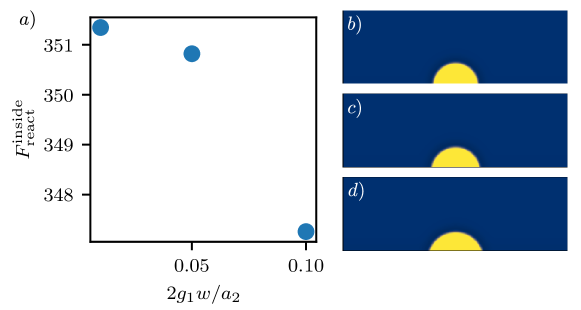
Figure 11: (a) Reactive energy inside a droplet for different wall affinities. (b-d) Corresponding snapshots of droplets.

Appendix E Series expansion of reaction-diffusion fluxes

In the following, we want to approximate Eq. 5 of the main text by two reaction-diffusion equations. We approximate the state of the system by a concentration field inside ($c_{\mathrm{in}}$) and outside ($c_{\mathrm{out}}$) the droplet, which are connected by a thin interface. Since $c_{\mathrm{in}}$ and $c_{\mathrm{out}}$ show little variation in their respective phase, we can expand the chemical potential around the respective equilibrium concentration, $\mu(c_{i})\approx\partial_{c}\mu|_{c=c_{i}^{(0)}}(c-c_{i}^{(0)})$ Weber et al. (2019). Inserting this expression into Eq. 5 of the main text, we obtain the reaction-diffusion equation

$$\partial_{t}c_{i}=D\nabla^{2}c_{i}-k(c_{i}-c_{0})\;,\qquad i=\mathrm{in}/\mathrm{out}\;.$$ (34)

The diffusivity $D=\Lambda_{\mathrm{d}}f^{\prime\prime}(c_{\mathrm{in}}^{(0)})=\Lambda_{\mathrm{d}}f^{\prime\prime}(c_{\mathrm{out}}^{(0)})$ is the same in both phases in our model. Note that we also neglected the fourth order derivative since we assume low concentration variations. The geometry of the problem is depicted in Fig. 12. The expected droplet shape follows a circular segment (corresponding to the spherical cap in 3D) with an opening angle of $2\vartheta$, where $\vartheta$ is the contact angle. The distance between the origin of the circular segment and the droplet wall interface is given by $y_{0}=R\cos(\vartheta)$. Since we assume fast relaxation of the concentration fields inside each phase, we seek a steady state solution of Eq. (34). For the steady state equation ($\partial_{t}c=0$), it is instructive to define the reaction-diffusion length scale $L=\sqrt{D/k}$. The solution for the concentration field in the given polar geometry is given by Polyanin (2002)

$$c_{i}(r,{\varphi})=c_{0}+\sum_{n=0}^{\infty}\left[A_{n}^{i}I_{\lambda_{n}}\left(\frac{r}{L}\right)+B_{n}^{i}K_{\lambda_{n}}\left(\frac{r}{L}\right)\right]\cos(\lambda_{n}\bigl{(}{\varphi}-\vartheta)\bigr{)}\;,\qquad i=\mathrm{in}/\mathrm{out}\;.$$ (35)

Here, $I_{\lambda_{n}}(z)$ and $K_{\lambda_{n}}(z)$ are the modified Bessel functions of first and second kind, and $\lambda_{n}$ is the separation variable which has to fulfill $\lambda_{n}=n\pi/\vartheta$ to be consistent with the boundary conditions. We next will determine the coefficients $A_{n}^{i}$ and $B_{n}^{i}$ from the boundary conditions.

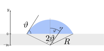
Figure 12: Geometry of a sessile droplet with attractive wall droplet interaction.

E.1 Concentration field inside the droplet

The relevant boundary conditions are

$$\left.\frac{\partial c}{\partial y}\right|_{y=0} =0 c(r=R) =c_{\mathrm{in}}^{(0)}+\beta_{\mathrm{in}}\gamma_{\mathrm{ds}}/R\;.$$ (36)

Translating the first boundary condition to polar coordinates gives

$$\left.\frac{\partial c(r(x,y),{\varphi}(x,y)}{\partial y}\right|_{0}=\frac{\partial c}{\partial r}\frac{\partial r}{\partial y}+\frac{\partial c}{\partial\varphi}\frac{\partial\varphi}{\partial y}=\left[\frac{\partial c}{\partial r}\cos({\varphi})-\frac{\partial c}{\partial{\varphi}}\frac{\sin({\varphi})}{r}\right]_{r_{0}({\varphi})=R\frac{\cos(\vartheta)}{\cos({\varphi})}}=0\;.$$ (37)

We rewrite the second boundary condition as

$$\sum_{n}A_{n}d_{n}({\varphi})+B_{n}e_{n}({\varphi})=c_{\mathrm{in}}^{(0)}+\beta_{\mathrm{in}}\gamma_{\mathrm{ds}}/R\;,$$ (38)

with

$$d_{n}({\varphi}) =I_{\lambda_{n}}(R/L)\cos({\lambda_{n}}{\varphi}) e_{n}({\varphi}) =K_{\lambda_{n}}(R/L)\cos({\lambda_{n}}{\varphi})\;.$$ (39)

Next, we define the projection operator

$$P[f]\equiv\int_{-\vartheta}^{\vartheta}f({\varphi})h_{m}({\varphi})\text{d}{\varphi}$$ (40)

for a well behaving function $h_{m}({\varphi})$, which will be defined explicitly later. Applying the projection operator to the boundary condition leads to

$$\sum_{n}\left[A^{n}\left(I_{\lambda_{n}}(R/L)\int_{-\vartheta}^{\vartheta}\cos({\lambda_{n}}{\varphi})h_{m}({\varphi})\text{d}{\varphi}\right)+B^{n}\left(K_{\lambda_{n}}(R/L)\int_{-\vartheta}^{\vartheta}\cos({\lambda_{n}}{\varphi})h_{m}({\varphi})\text{d}{\varphi}\right)\right]\\ =\left(c_{\mathrm{in}}^{(0)}+\frac{\beta_{\mathrm{in}}\gamma_{\mathrm{ds}}}{R}-c_{0}\right)\int_{-\vartheta}^{\vartheta}h_{m}({\varphi})\text{d}{\varphi}\;.$$ (41)

We rewrite this expression as

$$\sum_{n}(C_{mn}A_{n}+D_{mn}B_{n})=b_{m}\;\Leftrightarrow\;\mathbf{C}A+\mathbf{D}B=b$$ (42)

with coefficients

$$C_{mn} =\int_{-\vartheta}^{\vartheta}d_{n}({\varphi})h_{m}({\varphi})\text{d}{\varphi}\;,$$ (43a)

$$D_{mn} =\int_{-\vartheta}^{\vartheta}e_{n}({\varphi})h_{m}({\varphi})\text{d}{\varphi}\;,$$ (43b)

$$b_{m} =\left(c_{\mathrm{in}}^{(0)}+\frac{\beta_{\mathrm{in}}\gamma_{\mathrm{ds}}}{R}-c_{0}\right)\int_{-\vartheta}^{\vartheta}h_{m}({\varphi})\text{d}{\varphi}\;.$$ (43c)

Consequently, we recast the boundary condition into a system of linear equations. The number of equations is in principle infinite, but we can hope to obtain an accurate approximation by looking at finite number $m$ of modes. We want to treat the droplet-wall boundary condition in a similar way. We can insert the solution for the concentration field into the boundary condition and obtain

$$\sum_{n}\left[A^{n}\frac{I_{\lambda_{n}-1}\left(\frac{R\cos(\vartheta)}{L\cos({\varphi})}\right)+I_{\lambda_{n}+1}\left(\frac{R\cos(\vartheta)}{L\cos({\varphi})}\right)}{2L}-B^{n}\frac{K_{\lambda_{n}-1}\left(\frac{R\cos(\vartheta)}{L\cos({\varphi})}\right)+K_{\lambda_{n}+1}\left(\frac{R\cos(\vartheta)}{L\cos({\varphi})}\right)}{2L}\right]\cos(\lambda_{n}{\varphi})\\ +\sum_{n}\left[A^{n}I_{\lambda_{n}}\left(\frac{R\cos(\vartheta)}{L\cos({\varphi})}\right)+B^{n}K_{\lambda_{n}}\left(\frac{R\cos(\vartheta)}{L\cos({\varphi})}\right)\right]\frac{\sin(\lambda_{n}{\varphi})\sin({\varphi})}{R\cos(\vartheta)}=0\;,$$ (44)

which we rewrite as

$$\sum_{n}A_{n}f_{n}({\varphi})+B_{n}g_{n}({\varphi})=0\;,$$ (45)

with

$$f_{n}({\varphi}) =\frac{I_{\lambda_{n}-1}\left(\frac{R\cos(\vartheta)}{L\cos({\varphi})}\right)+I_{\lambda_{n}+1}\left(\frac{R\cos(\vartheta)}{L\cos({\varphi})}\right)}{2L}\cos(\lambda_{n}{\varphi})+I_{\lambda_{n}}\left(\frac{R\cos(\vartheta)}{L\cos({\varphi})}\right)\frac{\sin(\lambda_{n}{\varphi})\sin({\varphi})}{R\cos(\vartheta)}\;,$$ (46a)

$$g_{n}({\varphi}) =\frac{-K_{\lambda_{n}-1}\left(\frac{R\cos(\vartheta)}{L\cos({\varphi})}\right)-K_{\lambda_{n}+1}\left(\frac{R\cos(\vartheta)}{L\cos({\varphi})}\right)}{2L}\cos(\lambda_{n}{\varphi})+K_{\lambda_{n}}\left(\frac{R\cos(\vartheta)}{L\cos({\varphi})}\right)\frac{\sin(\lambda_{n}{\varphi})\sin({\varphi})}{R\cos(\vartheta)}\;.$$ (46b)

After applying the projection operator $P$, we then obtain another system of linear equations

$$\sum_{n}E_{mn}A_{n}+F_{mn}B_{n}=0\;\Leftrightarrow\mathbf{E}A+\mathbf{F}B=0\;,$$ (47)

where the coefficients are given by

$$E_{mn} =\int_{-\vartheta}^{\vartheta}f_{n}({\varphi})h_{m}({\varphi})\text{d}{\varphi}\;,$$ (48a)

$$F_{mn} =\int_{-\vartheta}^{\vartheta}g_{n}({\varphi})h_{m}({\varphi})\text{d}{\varphi}\;.$$ (48b)

Finally, the only task left to do is to solve the two matrix equations

$$\mathbf{C}A+\mathbf{D}B=b\;,$$ (49a)

$$\mathbf{E}A+\mathbf{F}B=0\;.$$ (49b)

We can combine both equations to

$${\scriptstyle\begin{pmatrix}\mathbf{C}&\mathbf{D}\\ \mathbf{E}&\mathbf{F}\end{pmatrix}\begin{pmatrix}A\\ B\end{pmatrix}=\begin{pmatrix}b\\ 0\end{pmatrix}\;,}$$ (50)

and invert the full matrix numerically. We choose $h_{m}({\varphi})=\cos(\pi m{\varphi}/\vartheta)$ in the projection operator and $m\in[0,3]$.

E.2 Concentration field outside the droplet

For the concentration profile outside we have in principle three boundary conditions

$$c(R) =c_{\mathrm{out}}^{(0)}+\beta_{\mathrm{out}}\gamma_{\mathrm{ds}}/R \left.\frac{\partial c}{\partial z}\right|_{z=z_{0}} =0 \lim_{r\rightarrow\infty}\frac{\partial c}{\partial r} =0\;.$$ (51)

The projection method we used before is not well suited for this situation since the first and the last boundary condition are defined over ${\varphi}\in[-\vartheta,\vartheta]$, whereas the second one is defined over ${\varphi}\in[-\pi/2,-\vartheta]\cup[\vartheta,\pi/2]$. We can define the operators over the specified range of ${\varphi}$ and get three equations for two unknowns, which gives an overdetermined system. One way around this is to consider a domain given by the opening angle $2\vartheta$. If we use the same quantization of the separation variable $\lambda=\pi n/\vartheta$, we can solve the problem with the two boundary conditions which are defined over the opening angle. Using the same operator as defined for the inside concentration we get the two equations

$$\mathbf{C}A+\mathbf{D}B =\mathbf{b}_{out}\;,$$ (52a)

$$\mathbf{G}A+\mathbf{H}B =0\;,$$ (52b)

where

$$G_{mn} =\int_{-\vartheta}^{\vartheta}k_{n}({\varphi})h_{m}({\varphi})\text{d}{\varphi}\;,$$ (53a)

$$H_{mn} =\int_{-\vartheta}^{\vartheta}l_{n}({\varphi})h_{m}({\varphi})\text{d}{\varphi}\;,$$ (53b)

$$b_{m}^{\mathrm{out}} =\left(c_{\mathrm{out}}^{(0)}+\frac{\beta_{\mathrm{in}}\gamma_{\mathrm{ds}}}{R}-c_{0}\right)\int_{-\vartheta}^{\vartheta}h_{m}({\varphi})\text{d}{\varphi}\;,$$ (53c)

with

$$k_{n}({\varphi}) =\frac{I_{\lambda_{n}-1}\left(\frac{R_{\infty}}{L}\right)+I_{\lambda_{n}+1}\left(\frac{R_{\infty}}{L}\right)}{2L}\cos(\lambda_{n}{\varphi})\;,$$ (54a)

$$l_{n}({\varphi}) =\frac{-K_{\lambda_{n}-1}\left(\frac{R_{\infty}}{L}\right)-K_{\lambda_{n}+1}\left(\frac{R_{\infty}}{L}\right)}{2L}\cos(\lambda_{n}{\varphi})\;.$$ (54b)

We can solve for the coefficients as before by inverting the combined matrix. Note that $\mathbf{b}_{\mathrm{out}}$ is defined as before but with a different constant value.

$${\scriptstyle\begin{pmatrix}\mathbf{C}&\mathbf{D}\\ \mathbf{G}&\mathbf{H}\end{pmatrix}\begin{pmatrix}A\\ B\end{pmatrix}=\begin{pmatrix}b_{\mathrm{out}}\\ 0\end{pmatrix}\;.}$$ (55)

E.3 Special case of a neutral wall

In the case of a neutral wall the opening angle is $2\vartheta=\pi$, and we obtain a slightly different matrix equation for the coefficient, which needs extra treatment.

E.3.1 Concentration field inside the droplet

The solution to the Helmholtz equation is still given by the concentration field

$$c(r,{\varphi})=c_{0}+\sum_{n=0}^{\infty}(A^{n}I_{\lambda}(r/L)+B^{n}K_{\lambda}(r/L))\cos(\lambda{\varphi})\;.$$ (56)

For the neutral wall, we obtain the boundary conditions for the concentration profile inside the droplet as

$$\left.\frac{\partial c}{\partial r}\right|_{r=0} =0 \left.\frac{\partial c}{\partial{\varphi}}\right|_{{\varphi}=\pm\pi/2} =0\;.$$ (57)

This allows us to eliminate $B^{n}=0$. The second boundary condition is already fulfilled by the choice of the separation variable $\lambda_{n}=n\pi/\vartheta$. We are left with the boundary condition

$${c}(R) =c_{\mathrm{in}}^{(0)}-c_{0}+\beta\mathrm{in}\gamma_{\mathrm{ds}}/R$$

$$=\sum_{n}A_{n}I_{\lambda_{n}}(R/L)\cos(\lambda_{n}{\varphi})=c_{\mathrm{in}}^{(0)}-c_{0}+\beta_{\mathrm{in}}\gamma_{\mathrm{ds}}/R\;.$$ (58)

We can then apply the projection $P$ operator and get

$$\begin{split}\sum_{n}A_{n}I_{\lambda_{n}}(R/L)\int_{-\pi/2}^{\pi/2}\cos(\lambda_{n}{\varphi})h_{m}({\varphi})\text{d}{\varphi}=(-c_{0}+\beta\gamma/R)\int_{-\pi/2}^{\pi/2}h_{m}({\varphi})\text{d}{\varphi}\end{split}$$ (59)

The corresponding matrix equation can be written as

$$\sum_{n}\bar{C}_{mn}A_{n}=b_{m}\;\Leftrightarrow\;\mathbf{\bar{C}}A=b$$ (60)

with coefficients

$$\bar{C}_{mn} =I_{\lambda_{n}}(R/L)\int_{-\pi/2}^{\pi/2}\cos(\lambda_{n}{\varphi})h_{m}({\varphi})\text{d}{\varphi}\;,$$ (61a)

$$b_{m} =(c_{\mathrm{in}}^{(0)}-c_{0}+\beta\gamma/R)\int_{-\pi/2}^{\pi/2}h_{m}({\varphi})\text{d}{\varphi}\;.$$ (61b)

E.3.2 Concentration field outside the droplet

The concentration outside $c_{\mathrm{out}}$ can now be solved for the full domain. Fortunately, the equations remain the same as in the case of an attractive wall, see Sec. E.2.

All matrix equations where then solved using numpy for the first four modes Harris et al. (2020).

Appendix F Reactions deform sessile 3D droplets

To test whether the observed droplet deformations also persist in 3D, we first performed simulations in Cartesian coordinates. Fig. 13 shows that we indeed find deformed, flattened droplet shapes as expected from our analysis in 2D. Since the simulations exhibit a cylindrical symmetry, we used cylindrical coordinates for the simulations shown in the main text to minimize the computational cost.

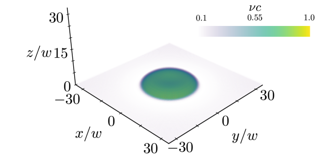
Figure 13: Concentration profile $c(x,y,z)$ of a stationary 3D droplet for reaction rate $k/k_{0}=0.0053$ and wall affinity $g_{1}=0.05a_{2}/w$. Simulations were performed in Cartesian coordinates using $L_{\mathrm{x}}=L_{\mathrm{y}}=64w$, $L_{\mathrm{z}}=32w$ with a discretization of $0.5w$.

Appendix G Electrostatic analogy explains effects of driven reactions

In this section, we investigate the equilibrium surrogate model given by Eq. (8) in the main text in detail, allowing us to interpret the reactions as long-ranged electrostatic interactions. By adopting this energy perspective, we can assess the conditions under which droplet deformation and droplet splitting might be favorable.

G.1 Geometry of the problem

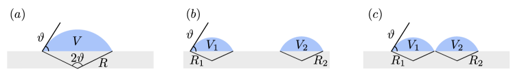
Figure 14: Geometry of the one droplet state (a) compared to the two separated droplets (b) and two connected droplets.

We want to compare the energy of the three scenarios depicted in Fig. 14: The first one consist of a single droplet (I), the second one consists of two smaller separated droplets (II), and the third one consists of two smaller adjacent droplets (II-c). We assume that the contact angle $\vartheta$ is constant and only depends on $g_{1}$ (as defined in the main text). Since we want to discuss the 2D and 3D case alongside, we introduce $V_{\mathrm{2D}}$ for the area of a circular segment and $V_{\mathrm{3D}}$ as the volume of a spherical cap. For a circular segment/spherical cap, we can calculate the volume $V$, the arc length $a$ (surface of sphere in 3D), and the chord length $c$ as (surface of droplet-wall interface),

$$V_{\mathrm{2D}} =\frac{R^{2}}{2}(2\vartheta-\sin(2\vartheta))\;, a_{\mathrm{2D}} =2\vartheta R\;, c_{\mathrm{2D}} =2R\sin(\vartheta)\;.$$ (62a)

$$V_{\mathrm{3D}} =\frac{\pi}{3}R^{3}(2+\cos(\vartheta))(1-\cos(\vartheta))^{2}\;, a_{\mathrm{3D}} =2\pi R^{2}(1-\cos(\vartheta))\;, c_{\mathrm{3D}} =\pi\sin^{2}(\vartheta)R^{2}\;.$$ (62b)

Since we assume constant total volume, we can relate the radii of the two smaller droplets ($R_{1}$ and $R_{2}$) to the radius of the single droplet by $R_{1}=R_{2}=R/\sqrt{2}$ in 2D and by $R_{1}=R_{2}=R/\sqrt[3]{2}$ in 3D. The distance between the centers of the two droplets is given by $l=2R_{1}\sin(\vartheta)$ for the adjacent droplets since we assume that they touch each other. For the separated droplets we assume no interaction between them. We consider a wall of length $L_{\mathrm{sys}}$.

G.2 Energy contributions for a single droplet

We expect that the behavior of the system is governed by three energy contributions: interfacial energy, volume energy, and a contribution that captures the influence of reactions. The volume energy is given by

$$E_{V}^{\mathrm{2D}} =-\Delta fV_{\mathrm{2D}}=-\Delta f\frac{R^{2}}{2}(2\vartheta-\sin(2\vartheta))\;,$$ (63a)

$$E_{V}^{\mathrm{3D}} =-\Delta fV_{\mathrm{3D}}=-\Delta f\frac{\pi}{3}R^{3}(2+\cos(\vartheta))(1-\cos(\vartheta))^{2}\;.$$ (63b)

The interfacial energy is given by $E_{\mathrm{int}}=\gamma_{\mathrm{ds}}a+\gamma_{\mathrm{wd}}c+\gamma_{\mathrm{ws}}(L_{\mathrm{sys}}-c)$. Since $\gamma_{\mathrm{ds}}\cos(\vartheta)=\gamma_{\mathrm{ws}}-\gamma_{\mathrm{wd}}$, we generally obtain $E_{\mathrm{int}}=\gamma_{\mathrm{ds}}(a-c\cos(\vartheta))+\gamma_{\mathrm{ws}}L_{\mathrm{sys}}$, which for the concrete systems read

$$E^{\mathrm{2D}}_{\mathrm{int}} =\gamma_{\mathrm{ds}}R(2\vartheta-\sin(2\vartheta))+\gamma_{\mathrm{ws}}L_{\mathrm{sys}}\;,$$ (64a)

$$E^{\mathrm{3D}}_{\mathrm{int}} =\gamma_{\mathrm{ds}}4\pi R^{2}\sin(\vartheta/2)^{4}+\gamma_{\mathrm{ws}}L_{\mathrm{sys}}\;.$$ (64b)

We can also express the interfacial energy as a function of the volume by substituting $R=\sqrt{2V^{\mathrm{2D}}/(2\vartheta-\sin(2\vartheta)}$ and $R=\left(\frac{3V_{\mathrm{3D}}}{\pi(2+\cos(\vartheta)(1-\cos(\vartheta)^{2})}\right)^{(2/3)}$,

$$E^{2D}_{\mathrm{int}} =\gamma_{\mathrm{ds}}\sqrt{2V_{\mathrm{2D}}(2\vartheta-\sin(2\vartheta))}\;,$$ (65a)

$$E^{3D}_{\mathrm{int}} =4\pi\left(\frac{3V_{\mathrm{3D}}}{\pi(2+\cos(\vartheta))(1-\cos(\vartheta)^{2})}\right)^{(2/3)}\sin^{4}(\vartheta/2)\;.$$ (65b)

The reactive energy can be determined from the electrostatic analogy, but we do not have a precise expression. To derive a scaling relation, we use the electrostatic energy of a droplet on a neutral wall, which serves as an upper bound for the energy of a spherical cap.

G.2.1 Energy of single chemically active droplet in dilute phase in two-dimensional system

As established in III.2, we can map the chemically active system onto an electrostatic system with the energy

$$F_{\mathrm{react}}=\frac{k}{2\Lambda_{\mathrm{d}}}\int(c-c_{0})\Psi\text{d}V\;,$$ (66)

with

$$\nabla^{2}\Psi=-(c-c_{0})\;.$$ (67)

We want to solve this equation and consequently need an expression for the concentration field, which we can approximate as solution to reaction-diffusion equations

$$\partial_{t}c_{i}=D\nabla^{2}c_{i}-k(c-c_{0})\;,~{}i\in\{\text{inside},\text{outside}\}$$ (68)

in stationary state, i.e., we assume quasi-stationarity. The solutions, with vanishing derivative at the origin and infinity and $c_{\mathrm{in}}(R)=c_{\mathrm{in}}^{(0)}$, $c_{\mathrm{out}}(R)=c_{\mathrm{out}}^{(0)}$, are given by

$$c_{\mathrm{in}}=c_{0}+(c_{\mathrm{in}}^{\mathrm{(0)}}-c_{0})\frac{I_{0}(r/L)}{I_{0}(R/L)}\;,$$ (69a)

$$c_{\mathrm{out}}=c_{0}+(c_{\mathrm{out}}^{\mathrm{(0)}}-c_{0})\frac{K_{0}(r/L)}{K_{0}(R/L)}\;,$$ (69b)

where $L=\sqrt{D/k}$ is the reaction-diffusion length scale as defined in the main text. These concentration profiles reproduce the main features of the solution to the full phase field equations. However, they do not conserve mass in the current form, which is easily seen by calculating the integrated reactive current inside and outside,

$$S_{\mathrm{in}} =-\frac{k2\pi(c_{\mathrm{in}}^{\mathrm{(0)}}-c_{0})}{I_{0}(R/L)}\int_{0}^{R}{I_{0}(r/L)}r\text{d}r=-\frac{k2\pi(c_{\mathrm{in}}^{\mathrm{(0)}}-c_{0})}{I_{0}(R/L)}LRI_{1}(\frac{R}{L})\;,$$ (70a)

$$S_{\mathrm{out}} =-\frac{k2\pi(c_{\mathrm{out}}^{\mathrm{(0)}}-c_{0})}{K_{0}(R/L)}\int_{R}^{\infty}{K_{0}(r/L)}r\text{d}r=-\frac{k2\pi(c_{\mathrm{out}}^{\mathrm{(0)}}-c_{0})}{K_{0}(R/L)}LRK_{1}(R/L)\;.$$ (70b)

This breaking of mass conservation is inconsistent with the initial equations Eq. (5) and Eq. (6) in the main text, which conserve the overall mass if the average density in the system is $c_{0}$. In contrast, the thin-interface model with quasi-stationary that we here use for simplicity breaks this mass conservation. Since this is a crucial feature of our system, we correct the mass by demanding a modified equilibrium concentration outside the droplet,

$$c_{\mathrm{out}}^{\mathrm{(0),mod}}=-(c_{\mathrm{in}}^{\mathrm{(0)}}-c_{0})\frac{I_{1}(R/L)K_{0}(R/L)}{I_{0}(R/L)K_{1}(R/L)}+c_{0}\;,$$ (71)

which we use in the following. We can then solve the energy integral

$$F_{\mathrm{react}}=\frac{k}{2\Lambda_{\mathrm{d}}}\int(c-c_{0})\Psi\text{d}V\;,$$ (72)

by rewriting it as

$$F_{\mathrm{react}}=-\frac{k}{2\Lambda_{\mathrm{d}}}\int(\nabla^{2}\Psi)\Psi\text{d}V\;.$$ (73)

The function $c-c_{0}$ is not continuous, so we integrate piecewise by parts

$$F_{\mathrm{react}} =-\frac{k}{2\Lambda_{\mathrm{d}}}\left(\int_{V_{\mathrm{in}}}(\nabla^{2}\Psi)\Psi\text{d}V+\int_{V_{\mathrm{out}}}(\nabla^{2}\Psi)\Psi\text{d}V\right)\;,$$

$$=-\frac{k}{2\Lambda_{\mathrm{d}}}\left(\int_{\partial V_{\mathrm{in}}}\Psi\nabla\Psi\mathbf{n}\text{d}A-\int_{V_{\mathrm{in}}}\nabla\Psi\nabla\Psi\text{d}V+\int_{\partial V_{\mathrm{out}}}\Psi\nabla\Psi\mathbf{n}\text{d}A-\int_{V_{\mathrm{out}}}\nabla\Psi\nabla\Psi\text{d}V\right)\;.$$ (74)

Using polar coordinates and the fact that we have Neumann conditions on $\Psi$ at $R=0$ and $R\to\infty$, we find

$$F_{\mathrm{react}}=-\frac{k}{2\Lambda_{\mathrm{d}}}\left(2\pi R(\Psi_{\mathrm{in}}\partial_{r}\Psi_{\mathrm{in}}-\Psi_{\mathrm{in}}\partial_{r}\Psi_{\mathrm{in}})-\int_{V_{\mathrm{in}}}(\partial_{r}\Psi_{\mathrm{in}})^{2}\text{d}V-\int_{V_{\mathrm{out}}}(\partial_{r}\Psi_{\mathrm{out}})^{2}\text{d}V\right)\;.$$ (75)

We next define the potential $\Omega=\partial_{r}\Psi$, plug it into the Poisson equation given by Eq. (67), and solve for $\Omega$,

$$\partial_{r}\Omega_{\mathrm{in}}+\frac{\Omega_{\mathrm{in}}}{r} =-(c_{\mathrm{in}}^{\mathrm{(0)}}-c_{0})\frac{I_{0}(r/L)}{I_{0}(R/L)}\;,$$ (76a)

$$\Omega_{\mathrm{in}} =\frac{d_{2}}{r}-(c_{\mathrm{in}}^{\mathrm{(0)}}-c_{0})\frac{I_{1}(r/L)L}{I_{0}(R/L)}\;,$$ (76b)

where $d_{2}$ is an integration constant. The constant $d_{2}$ needs to be zero since the field needs to be divergence-free at $r=0$. Similarly, we obtain

$$\Omega_{\mathrm{out}}=-\frac{L(c_{0}-{c_{\mathrm{out}}})K_{1}\left(\frac{r}{L}\right)}{K_{0}\left(\frac{R}{L}\right)}\;.$$ (77)

We immediately see that with the modified outside concentration we have $\Omega_{\mathrm{in}}(R)=\Omega_{\mathrm{out}}(R)$ and the boundary term in Eq. (75) vanish. Importantly, the boundary terms do not vanish by themselves but only after integration over full space. We thus find

$$F_{\mathrm{react}}=-\frac{k}{2\Lambda_{\mathrm{d}}}\left(-\int_{V_{\mathrm{in}}}(\partial_{r}\Psi_{\mathrm{in}})^{2}\text{d}V-\int_{V_{\mathrm{out}}}(\partial_{r}\Psi_{\mathrm{out}})^{2}\text{d}V\right)\;.$$ (78)

We then integrate the inside contribution of the energy,

$$F_{\mathrm{react}}^{\mathrm{in}} =\frac{2\pi k}{2\Lambda_{\mathrm{d}}}\int_{0}^{R}\Omega_{\mathrm{in}}^{2}r\text{d}r=\frac{2\pi k}{2\Lambda_{\mathrm{d}}}\left(\frac{(c_{\mathrm{in}}-c_{0})L}{I_{0}(R/L)}\right)^{2}\frac{1}{2}R\left(-RI_{0}\left(\frac{R}{L}\right){}^{2}+2LI_{1}\left(\frac{R}{L}\right)I_{0}\left(\frac{R}{L}\right)+RI_{1}\left(\frac{R}{L}\right){}^{2}\right)\;,$$

$$\approx\frac{\pi k}{16\Lambda_{\mathrm{d}}}\left(c_{\mathrm{in}}-c_{0}\right)^{2}R^{4}\;,$$ (79)

where the last approximation holds for small droplet radii $R$ and is in general a lower bound to the entire function. For the outside contribution we get

$$F_{\mathrm{react}}^{\mathrm{out}} =\frac{2\pi k}{2\Lambda_{\mathrm{d}}}\left(\frac{(c_{\mathrm{out}}-c_{0})L}{K_{0}(R/L)}\right)^{2}\int_{R}^{\infty}K_{1}(r/L)^{2}r\text{d}r\;,$$

$$=\frac{2\pi k}{2\Lambda_{\mathrm{d}}}\left(\frac{(c_{\mathrm{out}}-c_{0})L}{K_{0}(R/L)}\right)^{2}\left(\frac{1}{2}R\left(RK_{0}\left(\frac{R}{L}\right){}^{2}+2LK_{1}\left(\frac{R}{L}\right)K_{0}\left(\frac{R}{L}\right)-RK_{1}\left(\frac{R}{L}\right){}^{2}\right)\right)\;,$$

$$=\frac{\pi k}{\Lambda_{\mathrm{d}}}\left({(c_{\mathrm{out}}-c_{0})L}\right)^{2}R^{2}\left(\frac{1}{2}+L\frac{K_{1}\left(\frac{R}{L}\right)}{K_{0}\left(\frac{R}{L}\right)R}-\frac{1}{2}\frac{K_{1}\left(\frac{R}{L}\right){}^{2}}{K_{0}\left(\frac{R}{L}\right){}^{2}}\right)\;.$$ (80)

To determine the scaling behavior of this expression with $R$, we need to plug in the modified outside concentration

$$F_{\mathrm{react}}^{\mathrm{out}} =\frac{\pi k(c_{\mathrm{in}}^{\mathrm{(0)}}-c_{0})^{2}L^{2}}{\Lambda_{\mathrm{d}}}\left({\frac{I_{1}(R/L)K_{0}(R/L)}{I_{0}(R/L)K_{1}(R/L)}}\right)^{2}R^{2}\left(\frac{1}{2}+L\frac{K_{1}\left(\frac{R}{L}\right)}{K_{0}\left(\frac{R}{L}\right)R}-\frac{1}{2}\frac{K_{1}\left(\frac{R}{L}\right){}^{2}}{K_{0}\left(\frac{R}{L}\right){}^{2}}\right)\;$$

$$\approx\frac{\pi k(c_{\mathrm{in}}^{\mathrm{(0)}}-c_{0})^{2}}{\Lambda_{\mathrm{d}}8}{\left(2\log\left(\frac{2L}{R}\right)-(2\gamma_{\mathrm{euler}}+1)\right)}R^{4}$$ (81)

Consequently the total energy scaling is given by

$$F_{\mathrm{react}}^{\mathrm{tot}}=\frac{\pi k(c_{\mathrm{in}}^{\mathrm{(0)}}-c_{0})^{2}}{8\Lambda_{\mathrm{d}}}\left({2\log\left(\frac{2L}{R}\right)-(2\gamma_{\mathrm{euler}}+\frac{1}{2})}\right)R^{4}$$ (82)

where $\gamma_{\mathrm{euler}}\approx 0.577$ is the Euler number. This expression is again valid for small droplet radii but the approximation becomes unphysical as one approaches the reaction-diffusion length scale $L=\sqrt{D/k}$. The approximation then becomes negative, whereas the full expression approaches an almost linear positive increase.

G.2.2 Energy of single chemically active droplet in dilute phase in three-dimensional system

We perform the same calculations as above for three dimensions, which will give slight modifications. We again start from the two reaction-diffusion equations

$$\partial_{t}c_{i}=D\nabla^{2}c_{i}-k(c-c_{0});,~{}i\in\{\text{inside},\text{outside}\}.$$ (83)

We can write these equations in spherical coordinates and then solve for the stationary state

$$\partial_{r}^{2}c+\frac{2}{r}\partial_{r}c-\frac{1}{L^{2}}(c-c_{0})=0\;.$$ (84)

With boundary conditions $\partial rc_{\mathrm{in}}|_{r=0}=0$, $c(R)=c_{\mathrm{in}}$ the solution is given by

$$c_{\mathrm{in}}=\frac{R({c_{\mathrm{in}}^{\mathrm{(0)}}}-{c_{0}})\sinh\left(\frac{r}{L}\right)\text{csch}\left(\frac{R}{L}\right)}{r}+{c_{0}}\;.$$ (85)

For the outside, with boundary conditions $\lim_{r\to\infty}\partial_{r}c_{\mathrm{in}}|_{r=0}=0$ and $c(R)=c_{\mathrm{out}}^{\mathrm{(0)}}$, we find

$$c_{\mathrm{in}}=c_{0}+(c_{\mathrm{out}}^{\mathrm{(0)}}-c_{0})\frac{\exp((-r+R)/L)R}{r}\;.$$ (86)

From the concentration fields, we can next calculate the integrated reactive flux for the inside

$$S_{\mathrm{in}} =\int_{V_{\mathrm{in}}}-k(c_{\mathrm{in}}^{\mathrm{(0)}}-c_{0})\text{d}V\;,$$

$$=-4\pi kR\frac{(c_{\mathrm{in}}^{\mathrm{(0)}}-c_{0})}{\sinh(R/L)}\int_{0}^{R}\frac{\sinh(r/L)}{r}r^{2}\text{d}r\;,$$

$$=-4\pi kR\frac{(c_{\mathrm{in}}^{\mathrm{(0)}}-c_{0})}{\sinh(R/L)}L\left(R\cosh\left(\frac{R}{L}\right)-L\sinh\left(\frac{R}{L}\right)\right)\;,$$

$$=-4\pi kR{(c_{\mathrm{in}}^{\mathrm{(0)}}-c_{0})}L\left(R\coth\left(\frac{R}{L}\right)-L\right)\;,$$ (87)

and the outside

$$S_{\mathrm{out}} =\int_{V_{\mathrm{out}}}-k(c_{\mathrm{out}}-c_{0})\text{d}V\;,$$

$$=-4\pi k(c_{\mathrm{out}}^{\mathrm{(0)}}-c_{0})R\exp(R/L)\int_{R}^{\infty}\exp(-r/L)r\text{d}r\;,$$

$$=-4\pi k(c_{\mathrm{out}}^{\mathrm{(0)}}-c_{0})R\exp(R/L)L^{2}\;.$$ (88)

To balance the two fluxes, which ensures the solvability of the Poisson problem, we obtain a modified outside concentration,

$$c_{\mathrm{out}}^{\mathrm{(0),mod}} =\frac{(c_{\mathrm{in}}^{\mathrm{(0)}}-c_{0})}{\sinh(R/L)}\left(R\cosh\left(\frac{R}{L}\right)-L\sinh\left(\frac{R}{L}\right)\right)\frac{\exp(-R/L)}{L}+c_{0}\;,$$

$$=\frac{e^{-\frac{R}{L}}\left(c_{\text{in}}^{\text{(0)}}-c_{0}\right)\left(L-R\coth\left(\frac{R}{L}\right)\right)}{L}+c_{0}\;.$$ (89)

Next, we need to calculate the potential $\Omega=\partial_{r}\Psi$. We get for the inside

$$\Omega_{\mathrm{in}}=-\frac{R({c_{\mathrm{in}}^{\mathrm{(0)}}}-{c_{0}})}{\sinh(R/L)}\frac{Lr\cosh\left(\frac{r}{L}\right)-L^{2}\sinh\left(\frac{r}{L}\right)}{r^{2}}\;,$$ (90)

and for the outside

$$\Omega_{\mathrm{out}}=(c_{\mathrm{out}}^{\mathrm{(0)}}-c_{0}){\exp((R)/L)R}\frac{Le^{-\frac{r}{L}}(L+r)}{r^{2}}\;.$$ (91)

The inside energy is then given by

$$F_{\mathrm{react}}^{\mathrm{in}} =\frac{4\pi k}{\Lambda_{\mathrm{d}}2}\int_{0}^{R}\Omega^{2}r^{2}\text{d}r\;,$$

$$=\frac{4\pi k}{\Lambda_{\mathrm{d}}2}\left(\frac{RL(c_{\mathrm{in}}^{\mathrm{(0)}}-c_{0})}{\sinh(R/L)}\right)^{2}\int\frac{(r\cosh(r/L)-L\sinh(r/L))^{2}}{r^{2}}\text{d}r\;,$$

$$=\frac{\pi kL^{2}(c_{\mathrm{in}}^{\mathrm{(0)}}-c_{0})^{2}}{2\Lambda_{\mathrm{d}}}\left(\frac{R}{\sinh(R/L)}\right)^{2}\left(-\frac{4L^{2}\sinh^{2}\left(\frac{R}{L}\right)}{R}+L\sinh\left(\frac{2R}{L}\right)+2R\right)\;,$$

$$\approx\frac{\pi k(c_{\mathrm{in}}^{\mathrm{(0)}}-c_{0})^{2}}{2\Lambda_{\mathrm{d}}}\frac{4}{45}R^{5}\;,$$ (92)

where we expanded for small droplet radii in the last line. The outside energy can be expressed as

$$F_{\mathrm{react}}^{\mathrm{out}} =\frac{4\pi k}{\Lambda_{\mathrm{d}}2}\int_{0}^{R}\Omega^{2}r^{2}\text{d}r\;,$$

$$=\frac{4\pi k}{\Lambda_{\mathrm{d}}2}\left((c_{\mathrm{out}}^{\mathrm{(0)}}-c_{0}){\exp((R)/L)RL}\right)^{2}\int_{R}^{\infty}\left(\frac{e^{-\frac{r}{L}}(L+r)}{r^{2}}\right)^{2}r^{2}\text{d}r\;,$$

$$=\frac{4\pi k(c_{\mathrm{out}}^{\mathrm{(0)}}-c_{0})^{2}L^{2}}{\Lambda_{\mathrm{d}}2}\left({\exp((R)/L)R}\right)^{2}\frac{Le^{-\frac{2R}{L}}(2L+R)}{2R}\;,$$

$$=\frac{4\pi k(c_{\mathrm{out}}^{\mathrm{(0)}}-c_{0})^{2}L^{2}}{\Lambda_{\mathrm{d}}2}\left(L^{2}R+LR^{2}/2\right)\;.$$ (93)

Now, we still need to consider the modified outside concentration

$$c_{\mathrm{out}}=\frac{e^{-\frac{R}{L}}\left(c_{\text{in}}^{\text{(0)}}-c_{0}\right)\left(L-R\coth\left(\frac{R}{L}\right)\right)}{L}+c_{0}\;.$$ (94)

We then get

$$F_{\mathrm{react}}^{\mathrm{out}} =\frac{4\pi k(c_{\mathrm{in}}^{\mathrm{(0)}}-c_{0})^{2}L^{2}}{\Lambda_{\mathrm{d}}2}\left(\frac{e^{-\frac{R}{L}}\left(L-R\coth\left(\frac{R}{L}\right)\right)}{L}\right)^{2}\left(L^{2}R+LR^{2}/2\right)\;,$$

$$\approx\frac{2\pi k(c_{\mathrm{in}}^{\mathrm{(0)}}-c_{0})^{2}}{\Lambda_{\mathrm{d}}9}R^{5}\;,$$ (95)

where we expanded for small droplet radii in the last line. The total energy is thus given by

$$F_{\mathrm{react}}^{\mathrm{tot}}=\frac{4}{15}\frac{\pi k(c_{\mathrm{in}}^{\mathrm{(0)}}-c_{0})^{2}}{\Lambda_{\mathrm{d}}}R^{5}\;.$$ (96)

G.2.3 Approximation for sessile droplets

We now want to use the two expressions above to estimate the reactive energy $F_{\mathrm{react}}^{\text{sph.cap}}$ for sessile droplets forming a spherical cap on a wall. The volume of a spherical cap translates to its radius as

$$R^{2\mathrm{D}}(V) =\sqrt{2V^{2\mathrm{D}}/\pi}\;,$$ (97a)

$$R^{3\mathrm{D}}(V) =({3V^{3\mathrm{D}}/(2\pi)})^{\frac{1}{3}}\;.$$ (97b)

We can now insert these identities into the full expressions for the energy of a sessile droplet on an attractive wall to obtain an upper estimate for the energy of a neutral spherical cap. Note that we need to correct this energy by a factor of $\frac{1}{2}$ since we calculated the energy of a full droplets. Hence,

$$F_{\mathrm{react}}^{\text{sph.cap}}\approx\frac{1}{2}F_{\mathrm{react}}^{\mathrm{tot}}(R(V))\;,$$ (98)

where $F_{\mathrm{react}}^{\mathrm{tot}}$ is given by Eq. (82) for 2D and by Eq. (96) for 3D.

G.3 Energy contributions for two droplets

For the two-droplet scenarios, the energy scaling with the volume remains unchanged. For the interface contribution, we now need to consider two contributions with half of the total volume. We thus get

$$E^{2D}_{\mathrm{int}} =\sqrt{2}\gamma_{\mathrm{ds}}\sqrt{2V(2\vartheta-\sin(2\vartheta))}\;,$$ (99a)

$$E^{3D}_{\mathrm{int}} =\sqrt[3]{2}4\pi\left(\frac{3V^{\mathrm{3D}}}{\pi(2+\cos(\vartheta))(1-\cos(\vartheta)^{2})}\right)^{(2/3)}\sin^{4}(\vartheta/2)\;.$$ (99b)

The reactive energy can be calculated as follows

$$F^{\mathrm{2D}}_{\mathrm{react}} =b_{\mathrm{2D}}kV_{1}^{2}+b_{\mathrm{2D}}kV_{2}^{2}=2b_{\mathrm{2D}}k\left(\frac{V}{2}\right)^{2}=\frac{1}{2}bkV^{2}\;,$$ (100a)

$$F^{\mathrm{3D}}_{\mathrm{react}} =b_{\mathrm{3D}}kV_{1}^{(5/3)}+b_{\mathrm{3D}}kV_{2}^{(5/3)}=2b_{\mathrm{3D}}k\left(\frac{V}{2}\right)^{(5/3)}=\frac{\sqrt[3]{2}}{2}b_{\mathrm{3D}}kV^{(5/3)}\;.$$ (100b)

G.4 Energy of two interacting chemically active droplets

We next consider an additional energy contribution to describe the repulsion between the two adjacent droplets. To keep it simple, we approximate the two droplets as point charges with separation $l_{\mathrm{2D}}=2R_{1}\sin(\vartheta)=\sqrt{2}R\sin(\vartheta)$, and $l_{\mathrm{3D}}=2R_{1}\sin(\vartheta)=(2/\sqrt[3]{2})R\sin(\vartheta)$. The total charge inside each droplet is given by $q=\int(c_{0}-c(\mathbf{r}))dV\approx(c_{0}-c_{\mathrm{in}})V/2$ and the potential is

$$\Psi_{\mathrm{2D}} =\frac{1}{2\pi}q\log\left(|x|^{-1}\right)\;,$$ (101a)

$$\Psi_{\mathrm{3D}} =\frac{1}{4\pi}q(|x|)^{-1}\;,$$ (101b)

where we assume that the connection between the two droplet centers is along the $x$-axis and one charge is located at the origin. The associated energy to bring a charge from the boundary of the system to the position $l$ is then in 2D given by

$$F^{\mathrm{2D}}_{\mathrm{rep}} =\frac{k}{2\Lambda_{\mathrm{d}}}\int_{L_{\mathrm{sys}}}^{l}q\delta(-x)\Psi\text{d}x\;,$$

$$=\frac{k(c_{\mathrm{in}}-c_{0})^{2}V^{2}}{16\pi\Lambda_{\mathrm{d}}}\log(L_{\mathrm{sys}}/l)\;,$$

$$=\frac{k(c_{\mathrm{in}}-c_{0})^{2}}{16\pi\Lambda_{\mathrm{d}}}\log\left(L_{\mathrm{sys}}/\left(\sqrt{2}\sqrt{2V^{\mathrm{2D}}/(2\vartheta-\sin(2\vartheta)}\sin(\vartheta)\right)\right)V^{2}\;.$$ (102)

In three dimensions, we can safely assume an infinite system, such that the reference point of the potential vanishes. We consequently get

$$F^{\mathrm{3D}}_{\mathrm{rep}} =\frac{k(c_{\mathrm{in}}-c_{0})^{2}}{32\pi\Lambda_{\mathrm{d}}}\left((2/\sqrt[3]{2})\left(\frac{3V^{\mathrm{3D}}}{\pi(2+\cos(\vartheta)(1-\cos(\vartheta)^{2})}\right)^{(2/3)}\sin(\vartheta)\right)^{-1}V^{2}\;.$$ (103)

References

- Brangwynne et al. (2009) C. P. Brangwynne, C. R. Eckmann, D. S. Courson, A. Rybarska, C. Hoege, J. Gharakhani, F. Julicher, and A. A. Hyman, “Germline p granules are liquid droplets that localize by controlled dissolution/condensation,” Science 324, 1729–1732 (2009).
- Hyman, Weber, and Jülicher (2014) A. A. Hyman, C. A. Weber, and F. Jülicher, “Liquid-liquid phase separation in biology,” Annu. Rev. Cell Dev. Biol. 30, 39–58 (2014).
- Banani et al. (2017) S. F. Banani, H. O. Lee, A. A. Hyman, and M. K. Rosen, “Biomolecular condensates: organizers of cellular biochemistry,” Nature Reviews Molecular Cell Biology 18, 285–298 (2017).
- Dignon, Best, and Mittal (2020) G. L. Dignon, R. B. Best, and J. Mittal, “Biomolecular phase separation: From molecular driving forces to macroscopic properties,” Annu. Rev. Phys. Chem. 71, 53–75 (2020).
- Su, Mehta, and Zhang (2021) Q. Su, S. Mehta, and J. Zhang, “Liquid-liquid phase separation: Orchestrating cell signaling through time and space,” Molecular Cell 81, 4137–4146 (2021).
- Shimobayashi et al. (2021) S. F. Shimobayashi, P. Ronceray, D. W. Sanders, M. P. Haataja, and C. P. Brangwynne, “Nucleation landscape of biomolecular condensates,” Nature 599, 503–506 (2021).
- Böddeker et al. (2022) T. J. Böddeker, K. A. Rosowski, D. Berchtold, L. Emmanouilidis, Y. Han, F. H. T. Allain, R. W. Style, L. Pelkmans, and E. R. Dufresne, “Non-specific adhesive forces between filaments and membraneless organelles,” Nat. Phys. (2022).
- Böddeker et al. (2023) T. J. Böddeker, A. Rusch, K. Leeners, M. P. Murrell, and E. R. Dufresne, “Actin and microtubules position stress granules,” PRX Life 1, 023010 (2023).
- Zhao and Zhang (2020) Y. G. Zhao and H. Zhang, “Phase separation in membrane biology: The interplay between membrane-bound organelles and membraneless condensates,” Developmental Cell 55, 30–44 (2020).
- Kusumaatmaja et al. (2021) H. Kusumaatmaja, A. I. May, M. Feeney, J. F. McKenna, N. Mizushima, L. Frigerio, and R. L. Knorr, “Wetting of phase-separated droplets on plant vacuole membranes leads to a competition between tonoplast budding and nanotube formation,” Proceedings of the National Academy of Sciences 118, e2024109118 (2021).
- Beutel et al. (2019) O. Beutel, R. Maraspini, K. Pombo-García, C. Martin-Lemaitre, and A. Honigmann, “Phase separation of zonula occludens proteins drives formation of tight junctions,” Cell 179, 923–936.e11 (2019).
- Mangiarotti et al. (2023) A. Mangiarotti, N. Chen, Z. Zhao, R. Lipowsky, and R. Dimova, “Wetting and complex remodeling of membranes by biomolecular condensates,” Nature Communications 14, 2809 (2023).
- Pombo-García, Martin-Lemaitre, and Honigmann (2022) K. Pombo-García, C. Martin-Lemaitre, and A. Honigmann, “Wetting of junctional condensates along the apical interface promotes tight junction belt formation,” (2022), 10.1101/2022.12.16.520750.
- Gennes, Brochard-Wyart, and Quéré (2004) P.-G. Gennes, F. Brochard-Wyart, and D. Quéré, “Capillarity and wetting phenomena,” (2004).
- Young (1805) T. Young, “Iii. an essay on the cohesion of fluids,” Philosophical Transactions of the Royal Society of London 95, 65–87 (1805), https://royalsocietypublishing.org/doi/pdf/10.1098/rstl.1805.0005 .
- Cahn (1977) J. W. Cahn, “Critical point wetting,” 66 (1977).
- De Gennes (1981) P. G. De Gennes, “Polymer solutions near an interface. adsorption and depletion layers,” Macromolecules 14, 1637–1644 (1981).
- Zhang et al. (2012) R. Zhang, A. Khalizov, L. Wang, M. Hu, and W. Xu, “Nucleation and growth of nanoparticles in the atmosphere,” Chemical Reviews 112, 1957–2011 (2012).
- Hondele et al. (2019) M. Hondele, R. Sachdev, S. Heinrich, J. Wang, P. Vallotton, B. M. A. Fontoura, and K. Weis, “Dead-box atpases are global regulators of phase-separated organelles,” Nature 573, 144–148 (2019).
- Söding et al. (2019) J. Söding, D. Zwicker, S. Sohrabi-Jahromi, M. Boehning, and J. Kirschbaum, “Mechanisms for active regulation of biomolecular condensates,” Trends in Cell Biology , S0962892419301795 (2019).
- Kirschbaum and Zwicker (2021) J. Kirschbaum and D. Zwicker, “Controlling biomolecular condensates via chemical reactions,” Journal of The Royal Society Interface 18, 20210255 (2021).
- Zwicker, Hyman, and Jülicher (2015) D. Zwicker, A. A. Hyman, and F. Jülicher, “Suppression of ostwald ripening in active emulsions,” Physical Review E 92, 012317 (2015).
- Zwicker et al. (2017) D. Zwicker, R. Seyboldt, C. A. Weber, A. A. Hyman, and F. Jülicher, “Growth and division of active droplets provides a model for protocells,” Nat. Phys. 13, 408–413 (2017).
- Ziethen, Kirschbaum, and Zwicker (2023) N. Ziethen, J. Kirschbaum, and D. Zwicker, “Nucleation of chemically active droplets,” Physical Review Letters 130, 248201 (2023).
- Liese et al. (2023) S. Liese, X. Zhao, C. A. Weber, and F. Jülicher, “Chemically active wetting,” (2023), arXiv:2312.07239 [cond-mat.soft] .
- Cook (1970) H. Cook, “Brownian motion in spinodal decomposition,” Acta Metallurgica 18, 297–306 (1970).
- (27) J. W. Cahn and J. E. Hilliard, “Free energy of a nonuniform system. iii. nucleation in a two-component incompressible fluid,” , 13.
- de Gennes (1985) P. G. de Gennes, “Wetting: statics and dynamics,” Reviews of Modern Physics 57, 827–863 (1985).
- Weber et al. (2019) C. A. Weber, D. Zwicker, F. Jülicher, and C. F. Lee, “Physics of active emulsions,” Reports on Progress in Physics 82, 064601 (2019), arXiv: 1806.09552.
- Jülicher, Grill, and Salbreux (2018) F. Jülicher, S. W. Grill, and G. Salbreux, “Hydrodynamic theory of active matter,” Reports on Progress in Physics 81, 076601 (2018).
- De Groot and Mazur (1984) S. R. De Groot and P. Mazur, Non-equilibrium thermodynamics (NY: Dover Publications, 1984).
- God (1991) Solids far from equilibium, Collection Aléa-Saclay (Cambridge University Press, Cambridge ; New York, 1991).
- Zwicker (2020) D. Zwicker, “py-pde: A python package for solving partial differential equations,” Journal of Open Source Software 5, 2158 (2020).
- Kalikmanov (2013) V. Kalikmanov, “Nucleation theory,” Lecture Notes in Physics 860, 1–331 (2013).
- Liu and Goldenfeld (1989) F. Liu and N. Goldenfeld, “Dynamics of phase separation in block copolymer melts,” Physical Review A 39, 4805–4810 (1989).
- Christensen, Elder, and Fogedby (1996) J. J. Christensen, K. Elder, and H. C. Fogedby, “Phase segregation dynamics of a chemically reactive binary mixture,” Physical Review E 54, R2212–R2215 (1996).
- Muratov (2002) C. B. Muratov, “Theory of domain patterns in systems with long-range interactions of coulomb type,” Physical Review E 66, 066108 (2002).
- Rayleigh (1882) L. Rayleigh, “On the equilibrium of liquid conducting masses charged with electricity’, lond,” Philos. Mag. 14, 184–186 (1882).
- Golestanian (2017) R. Golestanian, “Origin of life: Division for multiplication,” Nat. Phys. 13, 323–324 (2017).
- Mao et al. (2018) S. Mao, D. Kuldinow, M. Haataja, and A. Košmrlj, “Phase behavior and morphology of multicomponent liquid mixtures,” Soft Matter 15, 1297 (2018).
- Zwicker and Laan (2022) D. Zwicker and L. Laan, “Evolved interactions stabilize many coexisting phases in multicomponent liquids,” Proceedings of the National Academy of Sciences 119, e2201250119 (2022).
- Zwicker (2022) D. Zwicker, “The intertwined physics of active chemical reactions and phase separation,” Curr. Opin. Colloid Interface Sci. 61, 101606 (2022).
- Agudo-Canalejo et al. (2021) J. Agudo-Canalejo, S. W. Schultz, H. Chino, S. M. Migliano, C. Saito, I. Koyama-Honda, H. Stenmark, A. Brech, A. I. May, N. Mizushima, and R. L. Knorr, “Wetting regulates autophagy of phase-separated compartments and the cytosol,” Nature 591, 142–146 (2021).
- Mokbel et al. (2023) M. Mokbel, D. Mokbel, S. Liese, C. A. Weber, and S. Aland, “A simulation method for the wetting dynamics of liquid droplets on deformable membranes,” (2023).
- Snead and Gladfelter (2019) W. T. Snead and A. S. Gladfelter, “The control centers of biomolecular phase separation: How membrane surfaces, ptms, and active processes regulate condensation,” Mol. Cell (2019), 10.1016/j.molcel.2019.09.016.
- Turci and Wilding (2021) F. Turci and N. B. Wilding, “Wetting transition of active brownian particles on a thin membrane,” Physical Review Letters 127, 238002 (2021).
- Turci, Jack, and Wilding (2023) F. Turci, R. L. Jack, and N. B. Wilding, “Partial and complete wetting of droplets of active brownian particles,” (2023), arXiv:2310.07531 [cond-mat].
- van der Walt et al. (2014) S. van der Walt, J. L. Schönberger, J. Nunez-Iglesias, F. Boulogne, J. D. Warner, N. Yager, E. Gouillart, T. Yu, and the scikit-image contributors, “scikit-image: image processing in Python,” PeerJ 2, e453 (2014).
- Goldman (2005) R. Goldman, “Curvature formulas for implicit curves and surfaces,” Computer Aided Geometric Design 22, 632–658 (2005).
- Polyanin (2002) A. D. Polyanin, Handbook of linear partial differential equations for engineers and scientists (Chapman & Hall/CRC, Boca Raton, 2002).
- Harris et al. (2020) C. R. Harris, K. J. Millman, S. J. van der Walt, R. Gommers, P. Virtanen, D. Cournapeau, E. Wieser, J. Taylor, S. Berg, N. J. Smith, R. Kern, M. Picus, S. Hoyer, M. H. van Kerkwijk, M. Brett, A. Haldane, J. F. del Río, M. Wiebe, P. Peterson, P. Gérard-Marchant, K. Sheppard, T. Reddy, W. Weckesser, H. Abbasi, C. Gohlke, and T. E. Oliphant, “Array programming with NumPy,” Nature 585, 357–362 (2020).