SM⁴Depth: Seamless Monocular Metric Depth Estimation
across Multiple Cameras and Scenes by One Model

Abstract

The generalization of monocular metric depth estimation (MMDE) has been a longstanding challenge. Recent methods made progress by combining relative and metric depth or aligning input image focal length. However, they are still beset by challenges in camera, scene, and data levels: (1) Sensitivity to different cameras; (2) Inconsistent accuracy across scenes; (3) Reliance on massive training data. This paper proposes SM⁴Depth, a seamless MMDE method, to address all the issues above within a single network. First, we reveal that a consistent field of view (FOV) is the key to resolve “metric ambiguity” across cameras, which guides us to propose a more straightforward preprocessing unit. Second, to achieve consistently high accuracy across scenes, we explicitly model the metric scale determination as discretizing the depth interval into bins and propose variation-based unnormalized depth bins. This method bridges the depth gap of diverse scenes by reducing the ambiguity of the conventional metric bin. Third, to reduce the reliance on massive training data, we propose a “divide and conquer” solution. Instead of estimating directly from the vast solution space, the correct metric bins are estimated from multiple solution sub-spaces for complexity reduction. Finally, with just 150K RGB-D pairs and a consumer-grade GPU for training, SM⁴Depth achieves state-of-the-art performance on most previously unseen datasets, especially surpassing ZoeDepth and Metric3D on mRI_θ. The code can be found at https://github.com/1hao-Liu/SM4Depth.

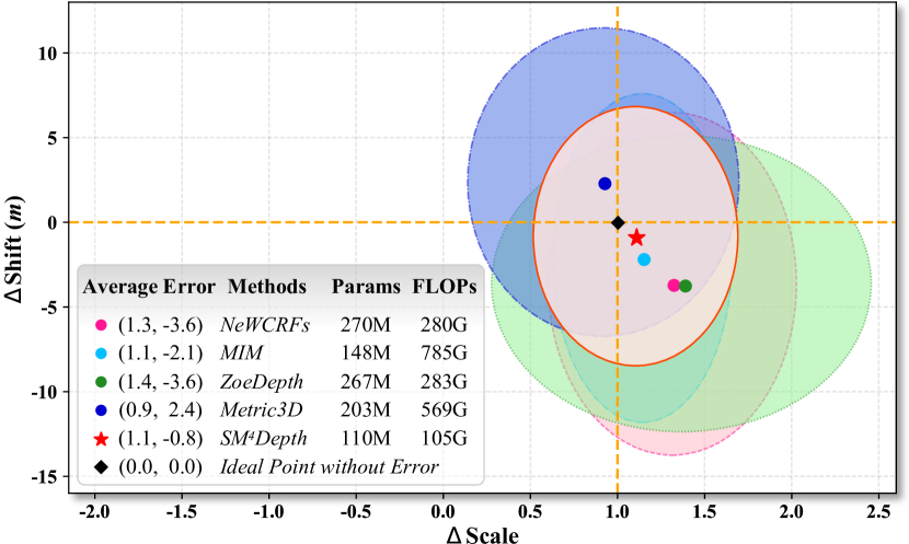
Figure 1: Confidence eclipses of $\Delta$scale and $\Delta$shift(m) between the prediction and the ground truth for all data in multiple zero-shot datasets (iBims-1[22], DIODE[46], nuScenes-val[7], DDAD[18], and ETH3D[39]).

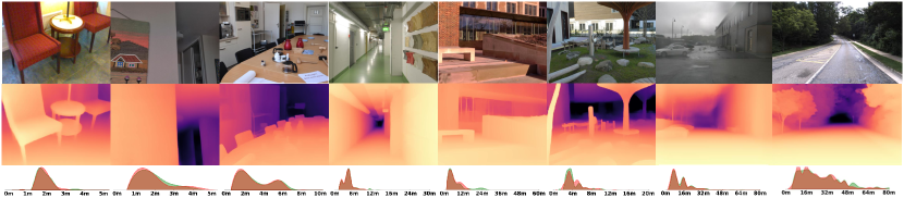
Figure 2: Depth and distribution visualization of SM⁴Depth. Our method enables good generalization across multiple metric depth datasets captured by different sensors. Top: input images. Middle: depth prediction. Bottom: distribution of the prediction (red) and ground truth (green). Six datasets: SUN-RGBD[41], DIODE[46], iBims-1[22], ETH3D[39], nuScenes-val[7], and DDAD[18].

1 Introduction

Monocular depth estimation is a fundamental visual task with wide-ranging applications in navigation [42, 6], 3D reconstruction [28, 47], 3D object perception [19, 32], visual SLAM [52, 58], and human pose estimation [43, 33]. In this community, early research focused on MMDE [23, 8, 51], which were trained only on specific datasets. As a result, they suffered from poor generalization when applied to unseen datasets, which limited their applications in the real world. To solve this issue, much research shifted their focus to monocular relative depth estimation (MRDE) [26, 55, 36] while disregarding the metric scale. Leveraging diverse and easily accessible relative depth data, these studies have achieved impressive performance, enabling their application in scale-free tasks, such as image editing [30, 11] and image stylization [21, 29], but not scale-sensitive applications, e.g., obstacle avoidance [53, 50, 49], 3D reconstruction [44], and virtual reality [1].

Beyond these approaches, universal MMDE has recently gained prominence for its generalization capabilities, marked by ZoeDepth [5] and Metric3D [56]. The former combined relative depth pre-training and metric depth fine-tuning. The latter achieved higher generalization by training on 8M data at the same focal length. However, both of them still face challenges in the three aspects of MMDE:

1. Camera Level: The existing method [56] aligned all images to one focal length by maintaining a canonical camera space, which is not straightforward for a pre-processing unit.

2. Scene Level: Real-world scenes vary widely in depth, ranging from $[1m,2m]$ (indoor close-up) to $[0.5m,80m]$ (street scenes), making models tend to focus on specific scenes and causing inconsistent accuracy across scenes. As depicted in Fig. 1, the previous works suffered from large accuracy fluctuations and high average errors.

3. Data Level: The reliance on massive training data (8M metric depth data for Metric3D) remains due to the high complexity of determining a unique metric scale from a vast solution space of the natural scene.

Aiming to address these issues, we propose a Seamless Model for MMDE across Multiple cameras and scenes (SM⁴Depth for short). First, to be compatible with all cameras, we analyze the key role of FOV in solving the metric ambiguity, which guides us to design a more straightforward FOV alignment unit for consistent inputs. For the second issue, we explicitly model metric scale determination as discretizing the depth interval into bins [3], and propose variation-based unnormalized bins. This method reduces the bin ambiguity between images which was inherent in previous width-based bins. This facilitates the learning of large-gap depth ranges from diverse scenes. Regarding the third issue, we propose a domain-aware bin estimation mechanism based on the “divide and conquer” idea, which estimates metric bins from various solution sub-spaces, not the entire one, for reducing complexity. Divide: we divide the common depth range into several range domains (RDs) offline and generate independent metric bins for each RD online. Conquer: we predict the RD that the input image belongs to, and weightedly fuse all bins into a single one. By solving all three issues, SM⁴Depth obtains correct depth distributions and ranges in all scenes displayed in Fig. 2.

Our primary contributions are as follows:

1. Camera level: We delve deep into the factor of “metric ambiguity”, and deduce the crucial role of FOV consistency. This sparks the design of our FOV alignment unit, which is more efficient than the previous one.

2. Scene level: To facilitate depth learning across scenes, we reveal the previously omitted bin ambiguity. This inspires us to propose the variation-based depth bins that bridge the gaps in scenes by reducing this ambiguity.

3. Data level: We propose the domain-aware bin estimation mechanism inspired by the “divide and conquer” idea. It reduces the complexity of metric bin estimation and thus eliminates the need for massive training data.

4. SM⁴Depth achieves state-of-the-art zero-shot performance but is trained on only 150K RGB-D pairs without needing a GPU cluster. With the aid of these accomplishments, SM⁴Depth significantly enhances the practical applicability of MMDE.

2 Related Work

Monocular metric depth estimation is a classic visual task, in which determining metric scales is a crucial point, and there are two paradigms. Mainstream MMDE methods [14, 23, 51, 8, 56] have directly modeled this task as a pixel-wise regression problem (predicting continuous depth values in the real metric space), where metric scales are implicitly encoded. In contrast, since [17], several methods [40, 3, 4] have defined this task as a classification problem. Among them, Adabins [3] explicitly encoded the metric scale into image-level depth bins. We follow the latter paradigm as this paper focuses on recovering metric scale. However, the same bin on two images with a large gap in depth range represents drastically different depths, causing misleading back-propagation during training. In this paper, we introduce variation-based bins to overcome this issue.

Zero-shot generation has become a new trend of monocular depth estimation in recent years. Early works [26, 34, 35] mainly achieved this goal by training with more accessible relative depth data. Initially, Li et al. [26] developed a pipeline of MRDE on large-scale relative depth data. Ranftl et al. [34] trained an MRDE model on five datasets and re-applied the training strategy to [35]. For high practicality, the universal MMDE was first proposed in [5] which combined relative depth and metric depth to achieve generalization. Yin et al. [56] trained the model on 8M metric depth data for generalization. This reliance on numerous training data is due to the complexity of determining correct metric scales from diverse natural scenes. Our approach aims to reduce the reliance on training data.

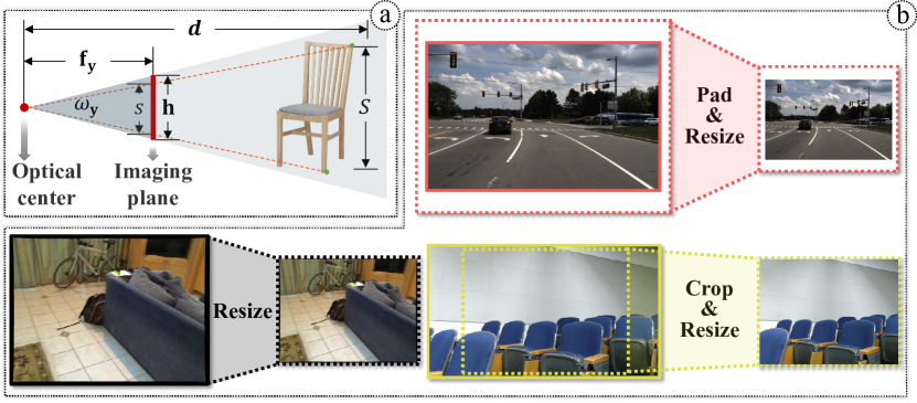
Figure 3: Principle and examples of FOV Alignment. (a) Side view of the pinhole camera model. (b) Cases of FOV alignment.

3 Problem Analysis and Countermeasures

In this section, we delve deep into the three issues of MMDE at the camera, scene, and data levels, and provide specific solutions for each issue.

3.1 Camera level: Sensitivity to Different Cameras

Analysis of metric ambiguity. According to Metric3D [56], due to different intrinsic parameters, two cameras produce different projections when observing an object at the same distance, which is well known as “metric ambiguity”. Next, we investigate the key of eliminating metric ambiguity by Fig. 3 that illustrates the imaging process of the pinhole camera model. Assuming that $d$ denotes the depth of the object, and $\mathbf{f_{y}}$ denotes the Y-direction focal length of the camera, measured in pixels. According to the similarity principle, there is an equation:

$$\frac{d}{S}=\frac{\mathbf{f_{y}}}{s}$$ (1)

where $S$ and $s$ are the actual height (in millimeters) and the imaging height (in pixels) of the object respectively. Based on Eq. (1), the object’s depth can be formulated as $d=S\big{[}\frac{\mathbf{f_{y}}}{s}\big{]}$. Therefore, a fixed value of $\big{[}\frac{\mathbf{f_{y}}}{s}\big{]}$ is crucial for a consistent depth $d$ across different cameras. In practice, all images need to be resized into the same resolution before being fed into the deep network:

$$d=S\Big{[}\frac{(\mathbf{f_{y}^{{}^{\prime}}}/\mathbf{f_{y}})\mathbf{f_{y}}}{(\mathbf{h}^{{}^{\prime}}/\mathbf{h})s}\Big{]}$$ (2)

where $\mathbf{f_{y}^{{}^{\prime}}}$ and $\mathbf{h}^{{}^{\prime}}$ are the focal length and height of the network input, $\mathbf{h}$ is the original height of the image, and $(\mathbf{f_{y}^{{}^{\prime}}}/\mathbf{f_{y}})=(\mathbf{h}^{{}^{\prime}}/\mathbf{h})$. Note that, since $\mathbf{f_{y}^{{}^{\prime}}}$ and $\mathbf{h}^{{}^{\prime}}$ are two pre-set values, the consistency of $\frac{\mathbf{h}}{\mathbf{f_{y}}}$ ensures a consistent depth $d$ across different cameras. Furthermore, the value $\frac{\mathbf{h}}{\mathbf{f_{y}}}$ follows an arctangent function relationship with the camera’s vertical FOV denoted as $\omega_{\mathbf{y}}$:

$$\omega_{\mathbf{y}}=2\arctan(\frac{\mathbf{h}}{2\mathbf{f_{y}}})$$ (3)

Thus, the consistency of $\omega_{\mathbf{y}}$ is essential for consistent depth and eliminating metric ambiguity across different cameras. The same applies to horizontal FOV denoted as $\omega_{\mathbf{x}}$.

FOV alignment for solving metric ambiguity. Following the analysis above, we propose an FOV alignment unit to ensure input consistency across cameras. Given an input image $\mathbf{I}$ with focal length $(\mathbf{f_{x}},\mathbf{f_{y}})$, we first preset the input resolution of network as $(h,w)$ and define the target FOV as $(\omega^{{}^{\prime}}_{\mathbf{x}},\omega^{{}^{\prime}}_{\mathbf{y}})$ in radians. Then, according to Eq. (3), an rectangular region $I^{{}^{\prime}}\!\in\!\mathbb{R}^{h^{{}^{\prime}}\!\times w^{{}^{\prime}}\!\times 3}$ on $\mathbf{I}$ equivalent to the target FOV $(\omega^{{}^{\prime}}_{\mathbf{x}},\omega^{{}^{\prime}}_{\mathbf{y}})$ is calculated by:

$$\!\!w^{{}^{\prime}}=2\mathbf{f_{x}}\tan(\frac{\omega^{{}^{\prime}}_{\mathbf{x}}}{2})\,\,,\,\,h^{{}^{\prime}}=2\mathbf{f_{y}}\tan(\frac{\omega^{{}^{\prime}}_{\mathbf{y}}}{2})$$ (4)

Next, we crop this region $I^{{}^{\prime}}$ from the original image $\mathbf{I}$, and fill the pixels beyond $\mathbf{I}$ with 255. Finally, the region $I^{{}^{\prime}}$ is resized to the target resolution $(h,w)$ for generating a new image $I$ as input of the network, as shown in Fig. 3 (b). Unlike transforming images to the same intrinsic parameter [56], we aim to ensure consistent inputs by unifying the FOV of images, thus do not need to maintain a canonical camera space.

3.2 Scene level: Inconsistent Accuracy

Generally, real-world images exhibit vastly different depth ranges, e.g. $[1m,2m]$ for indoor close-up and $[0.5m,80m]$ for street scenes. Such a large gap causes the model to overly concentrate on specific scenes instead of all scenes, leading to inconsistent accuracy across different scenes. In this section, we solve this issue by novel depth bins that bridge the gap of metric scale representation across scenes. Before that, we briefly review the conventional depth bin [3] and outline its weakness.

Reviewing width-based depth bin and its weakness. Given the input image $I\!\in\!\mathbb{R}^{h\times w\times 3}$, Adabins [3] generates an $N$-channel probability map $P\in\mathbb{R}^{h\times w\times N}$ and a vector $c\in\mathbb{R}^{N\times 1}$ representing the centers of $N$ depth bins discreted from the depth interval, which are linearly combined to obtain a metric depth map $D\in\mathbb{R}^{h\times w}$:

$$D(i)=\sum\nolimits_{n=1}^{N}c_{n}P_{n}(i)$$ (5)

where $D(i)$ is the $i^{\text{th}}$ pixel’s predicted depth, and $P_{n}(i)$ denotes the probability for pixel $i$ that its depth is equal to the $n^{\text{th}}$ bin center $c_{n}$. In Eq. (5), the bin center $c_{n}$ is calculated by accumulating the width of each bin $b\in\mathbb{R}^{N\times 1}$:

$$c_{n}=d_{\text{min}}+\left(d_{\text{max}}-d_{\text{min}}\right)(b_{n}/2+\sum\nolimits_{j=1}^{n-1}b_{j})$$ (6)

where $b_{n}=(b^{{}^{\prime}}_{n}+\epsilon)/\sum_{i=1}^{N}(b^{{}^{\prime}}_{i}+\epsilon)$ denotes the normalized width of the $n^{\text{th}}$ depth bin, with $\epsilon=10^{-3}$ and $b^{{}^{\prime}}_{n}\in[0,+\infty)$ being the unnormalized width predicted through a feedforward neural network (FFN) with the ReLU activation function. During training, the bi-directional Chamfer loss [16] is employed to enforce the small width $b^{{}^{\prime}}$ within the interesting depth interval in the ground truth depth map $\mathbf{D}$:

$$\mathcal{L}_{bin}(c,\mathbf{D})=\sum_{\mathbf{d}\in\mathbf{D}}\!\min_{c_{n}\in c}\!||\mathbf{d}-c_{n}||^{2}+\sum_{c_{n}\in c}\!\min_{\mathbf{d}\in\mathbf{D}}\!||\mathbf{d}-c_{n}||^{2}$$ (7)

where $\mathbf{d}$ is the pixel’s correct depth.

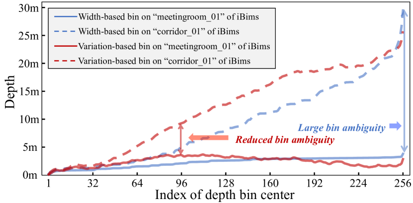
Figure 4: The bin center curves illustrate the bin ambiguity between a distant view image ($[0m,30m]$) and a close-up one ($[0m,3.5m]$). They are unnormalized, which was proved to have no effect in [3].

Since the depth width $b^{{}^{\prime}}_{n}$ is strictly positive, the bin centers $c_{n}$ increase monotonically with $n$ until approaching $d_{\text{max}}$, which enlarges the distinction in the bin center at the same index between two images. An excessive distinction would confuse the physical metric meaning of the probability map’s channels $P_{n}$. Thus, there is an ambiguity in pixel-wise classification when generating $P_{n}$, in turn leading to back-propagation of misleading signals during training. We term this phenomenon as “bin ambiguity”. As shown in Fig. 4, there is a significant difference between the same depth bin of the long-distance image (blue dashed line) and that of the close-up image (blue solid line).

Depth variation based bins for consistent accuracy. Our idea for reducing bin ambiguity is to use only the front part of the depth bin when the input image has a small depth range. To achieve this, we propose the variation-based unnormalized depth bins. Unlike the conventional bin $b^{{}^{\prime}}_{n}$, we use only an FFN without ReLU activation. In this way, the FFN outputs variations that allow negative values, denoted as $\hat{b}^{{}^{\prime}}\in\mathbb{R}^{N\times 1}$. Then, we re-formulate the bin center $c$ in Eq. (6) as an unnormalized bin center $\hat{c}$ to no longer be limited by the depth range of specific datasets (e.g., $[0m,10m]$ for NYUDv2 and $[0m,80m]$ for KITTI):

$$\hat{c}_{n}=\epsilon+\hat{b}_{n}^{{}^{\prime}}/2+\sum\nolimits_{j=1}^{n-1}\hat{b}_{j}^{{}^{\prime}}$$ (8)

Since the depth variations $\hat{b}^{{}^{\prime}}$ are allowed to be negative, the bin center value $\{\hat{c}_{n}|n\in[1,N]\}$ does not increase monotonically, as shown by the red lines in Fig. 4. In this way, the Chamfer loss (see Eq. (7)) forces an intermediate bin center $\hat{c}_{\mathbf{n}}(\mathbf{n}\!\!\in\!\![1,N])$ to have the maximum depth, not necessarily the last bin center $\hat{c}_{N}$. As a result, it reduces the ambiguity of the bins across different images, as indicated by the red double-headed arrows in Fig. 4. Specifically, since the front bin centers $\{\hat{c}_{n}|n\!\!\in\!\![1,\mathbf{n}]\}$ indicate depths from 0 to the maximum depth $d_{\text{max}}$, there is a lack of supervision for the latter bin centers $\{\hat{c}_{n}|n\!\!\in\!\!(\mathbf{n},N]\}$, causing them to be roughly suppressed below the maximum depth $d_{\text{max}}$. Consequently, the latter channels of the probability map $\{P_{n}|n\!\!\in\!\!(\mathbf{n},N]\}$ are filled with small values.

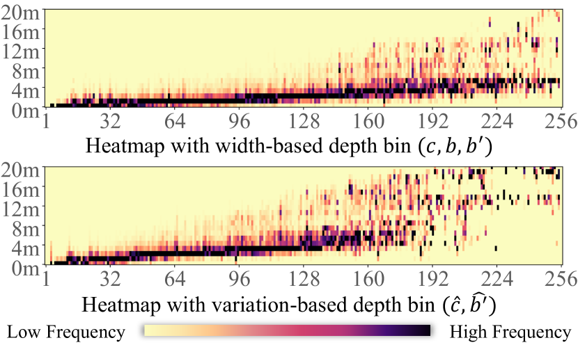
Figure 5: The heatmaps show the frequency of depth values occurring in each depth bin, which are obtained from iBims-1 [22]. If a square $(\mathcal{X},\mathcal{Y})$ appears darker, it indicates that the depth value $\mathcal{Y}$ mainly occurs within the $\mathcal{X}^{th}$ depth bin.

Fig. 5 presents additional statistics information, i.e., the frequency of depth values occurring in each depth bin. For the width-based depth bin $(c,b,b^{{}^{\prime}})$, depths below $4m$ occur most frequently across all bins. Conversely, variation-based depth bin $(\hat{c},\hat{b}^{{}^{\prime}})$ exhibits larger depths in the latter bins. This means that the depth values represented by each bin center are pulled apart on the level of the entire dataset, suppressing the bin ambiguity.

3.3 Data level: Reliance on Massive Training Data

Reason behind the reliance. Practical applications differ from specific datasets in that images are taken from various camera angles and innumerable scenes. Due to the diverse nature of appearance, mapping from visual cues to a wide range of depth values becomes highly intricate and cannot be exhaustively presented. Consequently, determining metric depth bins entails exploring a vast solution space, which necessitates greater attention to reducing its complexity. However, previous works have overlooked this crucial aspect by directly making prediction (e.g., [5] solves for metric bins and [56] predicts metric depth) from the entire solution space, inevitably requiring massive training data. To address this issue, we first divide the whole solution space into several sub-spaces. Then a “divide and conquer” method is proposed to generate metric bins in each sub-space and predict the best metric bins for the input.

Stage 1: Online depth range domain generation. To divide the solution space into sub-spaces, the previous approaches group all images according to semantic categories [5, 27]. However, a large gap in depth range may exist within one scene category. Unlike them, we group all training images according to the depth range that better constrains the camera angle and scene from which the image is taken.

According to [17], the amount of information for depth estimation decreases as the depth value increases. Thus, we employ a space-increasing strategy to gain more image groups (named range domain, RD) when the depth value is smaller. Assuming that the depth range is $[Z_{\text{min}},Z_{\text{max}}]$ and there are $K$ RDs, the $k^{\text{th}}$ RD can be formulated as:

$$RD_{k}=\Big{[}Z_{\text{min}},Z_{\text{min}}+\sum\nolimits_{i=1}^{k}{\frac{2i(Z_{\text{max}}-Z_{\text{min}})}{K(1+K)}}\Big{]}$$ (9)

We further visualize the RDs in the supplementary material.

Stage 2: Online domain-aware bin estimation design. We design a domain-aware bin estimation mechanism that generates metric bins for each RD and finds the best-matching metric bins, following the “divide and conquer” idea in two steps.

The “Divide” step aims to discretize each depth interval $RD_{k}$ into $N$ bins. Specifically, given the deep feature of the input image, we leverage a transformer encoder to learn the relationship between the deep feature and $K$ preset learnable 1-D embeddings (called bin queries). The output embeddings of these queries are fed into an FFN to generate $K$ depth variation vectors $\{\hat{b}^{{}^{\prime}[k]}|k\!\!\in\!\![1,K]\}$, and calculate the bin center vectors $\{\hat{c}^{[k]}|k\!\in\![1,K]\}$ based on Eq. (8). To illustrate our idea, we compare our design with two other possible choices:

• $1$ Query + $K$ FFNs: Using $K$ FFNs to process the output of only one query.

• $K$ Queries + $K$ FFNs: Using $K$ FFNs to process the outputs of $K$ queries in a one-to-one way.

• $K$ Queries + $1$ FFN (Ours): Using only one FFN to process the outputs of $K$ queries.

The first two designs both employ $K$ FFNs. Thus, each FFN only learns the knowledge of a single RD during training, which leads to drastically different outputs of these FFNs and makes them sensitive to input noise. The last design is recommended as the best choice and the experiments (in Sec.5.6) verify its superiority over other options.

The “Conquer” step aims to estimate the correct RD for the input image and determine the best-matching metric bins. Specifically, we preset an additional 1-D embedding (called domain query) alongside the bin queries. Its corresponding output is then fed into a classification head (CLS) to generate the probability that the input image belongs to each RD, denoted as $\{y_{k}\in[0,1]|k\in[1,K]\}$.

Subsequently, considering the possibility of images being positioned near the decision boundary of RD classification, we do not select the top-scoring metric bin but instead combine all bin center vectors $\hat{c}^{[k]}$ to a single one by using the RD probabilities $\{y_{k}|k\in[1,K]\}$ as weights:

$$\mathbf{c}=\sum\nolimits_{k\in[1,K]}\hat{c}^{[k]}y_{k}$$ (10)

where $\mathbf{c}$ is the final bin center vector.

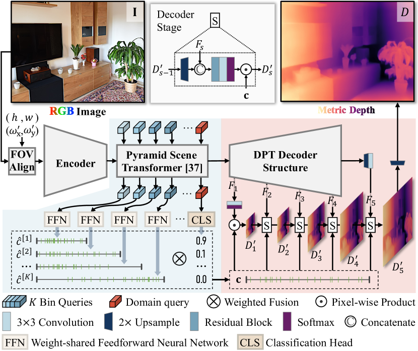
Figure 6: Pipeline of SM⁴Depth. The blue block denotes the domain-aware bin estimation. The red one denotes our decoder.

4 Architecture of SM⁴Depth

Pipeline. Fig. 6 illustrates the structure of our network. Given an RGB image $\mathbf{I}\!\in\!\mathbb{R}^{\mathbf{h}\times\mathbf{w}\times 3}$ and its pixel-presented focal length $(\mathbf{f_{x}},\mathbf{f_{y}})$, we use the FOV alignment unit (in Sec.3.1) to align $\mathbf{I}$ to a preset FOV $(\omega^{{}^{\prime}}_{\mathbf{x}},\omega^{{}^{\prime}}_{\mathbf{y}})$ and resolution $(h,w)$, obtaining an image without metric ambiguity $I\!\in\!\mathbb{R}^{h\times w\times 3}$. Then, we employ a Swin-Transformer as the encoder to extract the deep feature from $I$. Next, a pyramid scene transformer (PST) [40] is positioned between the encoder and decoder. It consists of three parallel transformer encoders with inputs of different patch sizes, respectively. We employ the transformer encoder with the smallest patch size to process all queries. Based on the mechanism in Sec.3.3, we obtain the bin center vector $\mathbf{c}$ of image $I$. Finally, we leverage a decoder with hierarchical scale constraints (HSC-Decoder) to anchor the metric scale in multiple resolutions and output the metric depth map $D$.

Categories	Method	SUN RGB-D				iBims-1 Benchmark				ETH3D Indoor				DIODE Indoor
		$\mathbf{\delta_{1}\uparrow}$	REL $\downarrow$	RMSE $\downarrow$	mRI${}_{\theta}\uparrow$	$\mathbf{\delta_{1}\uparrow}$	REL $\downarrow$	RMSE $\downarrow$	mRI${}_{\theta}\uparrow$	$\mathbf{\delta_{1}\uparrow}$	REL $\downarrow$	RMSE $\downarrow$	mRI${}_{\theta}\uparrow$	$\mathbf{\delta_{1}\uparrow}$	REL $\downarrow$	RMSE $\downarrow$	mRI${}_{\theta}\uparrow$
MMDE	BTS [24]	0.718	0.181	0.533	-31.45%	0.536	0.233	1.059	-32.82%	0.360	0.324	2.210	-18.73%	0.208	0.419	2.382	-34.57%
	AdaBins [3]	0.751	0.167	0.493	-23.07%	0.548	0.216	1.078	-29.56%	0.283	0.361	2.347	-31.23%	0.173	0.442	2.450	-40.95%
	NeWCRFs [57]	0.779	0.159	0.437	-14.67%	0.543	0.209	1.031	-26.43%	0.452	0.268	1.874	0.76%	0.183	0.402	2.307	-33.51%
	MIM [48]	0.844	0.147	0.341	0.00%	0.717	0.163	0.813	0.00%	0.453	0.287	1.800	0.00%	0.416	0.317	1.960	0.00%
Universal MMDE	ZoeD-N [5]	0.850	0.125	0.357	3.66%	0.652	0.171	0.883	-7.53%	0.388	0.275	1.678	-1.13%	0.376	0.331	2.198	-8.72%
	SM4Depth-N	0.874	0.121	0.303	10.80%	0.715	0.162	0.801	0.60%	0.486	0.249	1.662	9.40%	0.418	0.298	1.790	5.05%
	ZoeD-NK [5]	0.841	0.129	0.367	1.42%	0.610	0.189	0.952	-15.99%	0.353	0.280	1.691	-4.53%	0.386	0.335	2.211	-8.57%
	Metric3D[56]	0.033	2.631	5.633	×	0.818	0.158	0.582	15.18%	0.536	0.335	1.550	5.16%	0.505	0.427	1.687	0.21%
	SM4Depth	0.869	0.127	0.301	9.43%	0.790	0.134	0.673	15.06%	0.527	0.233	1.407	18.99%	0.356	0.300	1.721	1.04%
Categories	Method	nuScenes-val				DDAD				ETH3D Outdoor				DIODE Outdoor
		$\mathbf{\delta_{1}\uparrow}$	REL $\downarrow$	RMSE $\downarrow$	mRI${}_{\theta}\uparrow$	$\mathbf{\delta_{1}\uparrow}$	REL $\downarrow$	RMSE $\downarrow$	mRI${}_{\theta}\uparrow$	$\mathbf{\delta_{1}\uparrow}$	REL $\downarrow$	RMSE $\downarrow$	mRI${}_{\theta}\uparrow$	$\mathbf{\delta_{1}\uparrow}$	REL $\downarrow$	RMSE $\downarrow$	mRI${}_{\theta}\uparrow$
MMDE	BTS [24]	0.420	0.285	9.140	-9.24%	0.802	0.146	7.611	-13.07%	0.175	0.831	5.746	7.19%	0.172	0.838	10.475	-34.70%
	AdaBins [3]	0.483	0.272	10.178	-7.45%	0.757	0.155	8.673	-22.80%	0.110	0.889	6.480	-12.65%	0.162	0.853	10.322	-36.09%
	NeWCRFs [57]	0.415	0.280	7.402	-0.64%	0.866	0.120	6.359	2.66%	0.258	0.799	5.061	29.57%	0.177	0.841	9.304	-29.25%
	MIM [48]	0.396	0.283	6.868	0.00%	0.859	0.134	6.157	0.00%	0.159	0.889	6.048	0.00%	0.269	0.625	7.819	0.00%
Universal MMDE	ZoeD-K [5]	0.379	0.290	6.900	-2.41%	0.833	0.130	7.154	-5.41%	0.303	1.012	5.853	26.65%	0.269	0.823	6.891	-6.60%
	SM4Depth-K	0.623	0.229	7.175	23.98%	0.841	0.160	5.677	-4.56%	0.452	0.294	3.168	99.61%	0.280	0.552	8.335	3.06%
	ZoeD-NK [5]	0.371	0.299	6.988	-4.57%	0.821	0.139	7.274	-8.77%	0.337	0.752	4.758	49.56%	0.207	0.735	7.570	-12.49%
	Metric3D*[56]	0.868	0.143	8.506	48.27%	0.896	0.119	7.262	-0.01%	0.324	0.724	9.830	19.93%	0.169	0.499	9.353	-12.21%
	SM4Depth	0.672	0.214	7.221	29.65%	0.890	0.123	5.390	8.09%	0.348	0.273	3.274	78.01%	0.190	0.487	8.435	-5.05%

Table 1: Quantitative results on zero-shot datasets. mRI_θ denotes the mean relative improvement compared to MIM across all metrics($\delta_{1}$, REL, RMSE). All methods undergo evaluation consistently within a specific region. The best results are in bold and the second-best ones are underlined. $\times$ indicates poor performance. * means that Metric3D was trained on DDAD.

Decoder with hierarchical scale constraints. Our decoder draws inspiration from the refinement decoder structures [24, 8], but the divergence lies in scale constraints on the metric depth at each stage. As shown in Fig. 6, taking the PST’s output, denoted as $F_{1}$, as input, we employ the DPT’s decoder [35] to gradually recover the resolution of features, denoted as $F_{s}$ with a size $\frac{h}{2^{(6-s)}}\times\frac{w}{2^{(6-s)}}$, where $s\in\{1,2,3,4,5\}$ is the stage number. In the first stage, $F_{1}$ is compressed into $N$-channel and then multiplied pixel-wisely with $\mathbf{c}$ by Eq. (5), generating a low-resolution depth map $D^{{}^{\prime}}_{1}\in\mathbb{R}^{\frac{h}{32}\times\frac{w}{32}}$. In the following $s^{\text{th}}$ stage, the depth map of the former stage $D^{{}^{\prime}}_{s-1}$ is upsampled and fused with feature $F_{s}$ by a residual convolution block [8]. Then, we linearly combine the fused feature and the bin centers $\mathbf{c}$ to generate the depth map $D^{{}^{\prime}}_{s}\in\mathbb{R}^{\frac{h}{2^{(6-s)}}\times\frac{w}{2^{(6-s)}}}$. In this way, the depth map of the last stage $D^{{}^{\prime}}_{5}\in\mathbb{R}^{\frac{h}{2}\times\frac{w}{2}}$ is obtained. Compared to the previous refinement decoder [8], HSC-Decoder incorporates the metric bins into each stage to refine the depth range progressively, thus performing better in recovering the depth range. The loss functions are further described in the supplementary material.

5 Experiments

5.1 Datasets

Training. We randomly sample RGB-Depth pairs from various datasets for training. Specifically, we sample 24K pairs from ScanNet [13], 15K pairs from Hypersim [37], 51K pairs from DIML [10], 36K pairs from UASOL [2], 14K pairs from ApolloScape [20], and 11K pairs from CityScapes [12]. During training, NYUD [31] and KITTI [45] are used for validation. In addition, we apply the same pre-processing steps to the training data as [34, 5], elaborated in supplementary materials.

Testing. To evaluate the zero-shot performance, we employ eight datasets that are not used during the training process: SUN RGB-D [41], iBims-1 [22], ETH3D Indoor [38], DIODE Indoor [46] for indoor scene; nuScenes-val [7], DDAD [18], ETH3D Outdoor [38], DIODE Outdoor [46] for outdoor scene. Note that, we remove the test set of NYUD from SUN RGB-D to avoid unfair comparisons.

5.2 Metrics

We employ four widely used metrics [3] for evaluation: the accuracy under threshold ($\delta_{k}<1.25^{k},k=1,2,3$), the absolute relative error (REL), and the root mean squared error (RMSE). In addition, we use the relative improvement (RI) across datasets (mRI_η) and metrics (mRI_θ) in [5].

During the evaluation, the final output is obtained by averaging the predictions for an image and its mirror image. In addition, the final output is upsampled to match the original image size, and all metrics are computed within the same FOV. Note that, we cap the evaluation depth at 80m (compared to only 8m for SUN RGB-D and 10m for NYUD).

5.3 Implementation Details

SM⁴Depth employs the Swin Transformer Base as the backbone, and runs on a single NVIDIA RTX 3090 GPU. The network is trained by the Adam optimizer with parameters $(\beta_{1},\beta_{2})=(0.9,0.999)$. The training runs for 20 epochs with a batch size of 10. The initial learning rate is set to $2\times 10^{-5}$ and gradually reduced to $2\times 10^{-6}$. Note that, an over-large fixed FOV would cause too large invalid area in the small FOV dataset, making the network underfitting. We empirically set the fixed FOV to $(\omega^{{}^{\prime}}_{\mathbf{x}},\omega^{{}^{\prime}}_{\mathbf{y}})\!=\!(58^{\circ},45^{\circ})$ and the fixed resolution to $(w,h)\!=\!(564,424)$.

Method	Backbone	NYUD						RANK (mRIθ)
		$\mathbf{\delta_{1}\uparrow}$	$\mathbf{\delta_{2}\uparrow}$	$\mathbf{\delta_{3}\uparrow}$	REL$\downarrow$	RMSE$\downarrow$	log10$\downarrow$
ZoeD-N [5]	Beit-Large	0.956	0.995	0.999	0.075	0.279	0.032	1.00
ZoeD-NK [5]	Beit-Large	0.954	0.996	0.999	0.076	0.286	0.033	1.15
SM4Depth-N	Swin-Base	0.932	0.991	0.998	0.088	0.328	0.038	2.22
Metric3D [56]	ConvNeXt-Large	0.926	0.984	0.995	0.091	0.340	0.038	2.43
SM4Depth	Swin-Base	0.860	0.981	0.997	0.126	0.417	0.052	5.00
Method	Backbone	KITTI						RANK (mRIθ)
		$\mathbf{\delta_{1}\uparrow}$	$\mathbf{\delta_{2}\uparrow}$	$\mathbf{\delta_{3}\uparrow}$	REL$\downarrow$	RMSE$\downarrow$	log10$\downarrow$
ZoeD-K [5]	Beit-Large	0.978	0.998	0.999	0.049	2.221	0.021	1.00
ZoeD-NK [5]	Beit-Large	0.971	0.994	0.996	0.053	2.415	0.024	1.62
SM4Depth-K	Swin-Base	0.971	0.996	0.999	0.054	2.477	0.023	1.61
Metric3D [56]	ConvNeXt-Large	0.962	0.993	0.998	0.060	2.969	0.026	2.57
SM4Depth	Swin-Base	0.928	0.985	0.996	0.087	3.272	0.038	5.00

Table 2: Quantitative result on NYUD and KITTI. All methods undergo evaluation in a consistent region. The best results are in bold and the second-best ones are underlined.

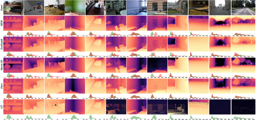
Figure 7: Qualitative comparison with MDE methods on zero-shot datasets. The depth distribution is under the depth maps with green for ground truth and red for prediction. Our method performs better on images with multiple viewpoints and diverse scenes.

5.4 Quantitative Result

We employ two classical MMDE methods, i.e., BTS [24] and AdaBins [3], as well as two more advanced MMDE approaches, i.e., NeWCRFs [57] and MIM [59], for comparison. Moreover, the universal MMDE methods, i.e., Metric3D [56] and ZoeDepth-N/K/NK [5], are also employed for comparison (N indicates NYUD fine-tuning and K for KITTI fine-tuning; they are also applicable to SM⁴Depth).

In Table 1, the upper part shows the zero-shot performance on four indoor datasets, and the lower part shows that on four outdoor datasets. Intuitively, our method outperforms most MMDE methods. Compared to Metric3D, SM⁴Depth performs better on most datasets, (i.e., SUN RGB-D, ETH3D, DIODE, and DDAD) and similar on iBims-1, but is only trained 150K images, which proves the effectiveness of SM⁴Depth. Especially, SM⁴Depth outperforms Metric3D by +58.08% and +8.10% mRI_θ on ETH3D Outdoor and DDAD. In addition, SM⁴Depth outperforms Metric3D on nuScenes-val by -1.285 of RMSE, but falls behind on $\delta_{1}$ and REL, as Metric3D is trained on much more self-driving datasets, which endows it an advantage in such scenes. Compared with ZoeDepth, SM⁴Depth leads on all datasets regardless of fine-tuning or not, not only in absolute metrics ($\delta_{1}$, RMSE) but also in relative metrics (REL), illustrating that SM⁴Depth learns more accurate relative depth from metric depth data. Note that, Metric3D shows a noticeable accuracy drop on SUN RGB-D, where all images are cropped beforehand. This degradation is due to the lack of constraint on the ratio $\frac{f}{\mathbf{h}}$ in Eq. (2). Specifically, the cropping operation alters the image size ($\mathbf{h},\mathbf{w}$), thereby invalidating this equation and resulting in a potential metric ambiguity in depth estimation. Furthermore, most methods struggle with accurate depth estimation on DIODE due to its high proportion of upward-perspective images that contain numerous invalid pixels.

Table 2 displays the results on NYUD and KITTI. In the comparison of the zero-shot setting, our method obtains lower $\delta_{1}$ and higher RMSE than Metric3D on NYUD and KITTI. However, after being fine-tuned on NYUD and KITTI, SM⁴Depth achieves competitive accuracy with the state-of-the-art methods, while avoiding a significant degradation in accuracy on zero-shot datasets (see in Table 1).

5.5 Qualitative Result

Fig. 7 visualizes several methods’ predictions and depth distributions. The $1^{\text{st}}-3^{\text{rd}}$ columns show close-up scenes with unusual perspectives, challenging depth range determination. Previous methods obtain the incorrect depth distributions, while Metric3D tends to push the background farther when the foreground boundary is clearly delineated. The $4^{\text{th}}-7^{\text{th}}$ columns show indoor scenes where other methods suffer from incorrect depth range, while SM⁴Depth recovers the depth distribution accurately, as our decoder optimizes the metric scale at multiple resolutions. The $8^{\text{th}}-10^{\text{th}}$ columns show multiple outdoor scenes. The predictions of MIM and ZoeDepth exhibit overall shifts, while Metric3D fails to distinctly differentiate between the front objects and the background wall. In contrast, due to training on multiple metric depth datasets, SM⁴Depth generates a visually reasonable depth distribution, while it does not assign an extreme depth value to sky regions because they are set to 0 during training. The last two columns show images from self-driving scenes. Although all methods generate good depth maps, SM⁴Depth obtains a more accurate depth distribution and captures richer shape details than other methods. Especially in the $12^{\text{th}}$ column, where objects are up to 80m away, our method correctly predicts their farthest depths as well as generating fine tree trunk edges.

Solutions	SUN RGB-D	ETH3D	DIODE	DDAD	mRIη $\uparrow$
CSTM_label [56]	1.051	2.648	5.950	28.094	0.00%
FOV Alignment	0.301	2.373	5.605	5.390	46.23%

Table 3: RMSE results using metirc ambiguity solutions on SM⁴Depth. The best results are in bold.

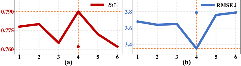
Figure 8: Parameter experiment about $K$. The performance, as measured by $\delta_{1}$ and RMSE, is optimal when $K$ equals 4. The dots represent the use of the uniform partition strategy for training.

5.6 Detail Analysis

Comparing metric ambiguity elimination methods. Metric3D [56] proposed two methods to solve metric ambiguity, i.e., CSTM_label and CSTM_image. However, only the code of CSTM_label is released. Thus, we employ CSTM_label to compare with our FOV alignment. As shown in Table 3, the proposed solution outperforms CSTM_label by +46.23% on the comprehensive metric mRI_η, especially on SUN RGB-D and DDAD. This performance gap arises from the cropping operation. Note that neither model was trained on DDAD, but the model using the CSTM_label appears to be incompatible with DDAD. This experiment proves the superiority of the FOV alignment in metric ambiguity elimination.

Number of depth range domain. We explore the optimal number of RD, i.e., $K$, and additionally evaluate the uniform partition strategy [17] when using the best $K$. Fig. 8 shows all variants’ performance on the mixing test sets. As $K$ increases, RMSE decreases slowly. RMSE suddenly drops below 3.4 when $K$ = 4, and rises again at 5 or 6. We argue that this phenomenon occurs because RDs better describe images with different appearance when $K$ = 4 and prevents excessive similarity between RDs due to redundant division. In addition, using the uniform partition strategy leads to a notable decrease in $\delta_{1}$ and RMSE.

Ablation study. We conduct the ablation study by gradually removing our designs and comparing all variants. In Table 4, the baseline (last row) consists of only an encoder-decoder structure and a PST [40]. Observably, the RMSEs increase overall as the proposed modules and innovations are gradually removed. The depth-variation based bins make the greatest contribution (+4.89% mRI_η), indicating its effectiveness in learning large depth range gaps. The entire domain aware bin estimation increases mRI_η by 2.36%, with the weighted fusion scheme contributing 1.5% of this. In addition, the HSC-decoder improves mRI_η by 3.67%.

Comparing designs for domain-aware bin estimation. As shown in Table 5, we compare three design choices of our domain-aware bin estimation mentioned in Sec.3.3 on the same four datasets in the ablation study. Compared to the other settings, “$K$*Query+$1$*FFN” achieves the lowest RMSE and highest mRI_η. The reason is that the single FFN is trained on multiple RDs and thus learns common knowledge for bin estimation from multiple RDs.

V-Bin1	WF-Bin2.1	DBE2.2	HSC3	iBims-1	ETH3D	DIODE	DDAD	mRIη $\uparrow$
$\surd$	$\surd$	$\surd$	$\surd$	0.673	2.373	5.605	5.390	10.92%
$\times$	$\surd$	$\surd$	$\surd$	0.692	2.504	6.033	5.726	6.03%
$\times$	$\times$	$\surd$	$\surd$	0.701	2.692	6.111	5.486	4.53%
$\times$	$\times$	$\times$	$\surd$	0.741	2.566	6.163	5.587	3.67%
$\times$	$\times$	$\times$	$\times$	0.695	2.695	6.107	6.767	0.00%
1: Depth-Variation based Bin			2.2: Domain-aware Bin Estimation
2.1: Weighted Fusion of Bins			3: Decoder with Hierarchical Scale Constraints

Table 4: RMSE results of the ablation study. The best results are in bold, while the second-best ones are underlined.

Design Choices	iBims-1	ETH3D	DIODE	DDAD	mRIη $\uparrow$
$1$   * Query   + $K$ * FFNs	0.770	2.522	5.982	6.601	0.00%
$K$ * Queries + $K$ * FFNs	0.734	2.401	5.820	6.920	1.84%
$K$ * Queries + $1$  * FFN	0.673	2.373	5.605	5.390	10.79%

Table 5: RMSE results of the domain-ware bin estimation. The best results are in bold, while the second-best ones are underlined.

6 Conclusion

In this paper, we address three issues of MMDE. At the camera level, we analyze the key role of FOV in resolving metric ambiguity, and propose a more straightforward pre-processing unit. At the scene level, we discuss the inherent issue of the bin-based methods when learning depth range with large discrepancies, that is the large inconsistency of the same bin in different images. To address this issue, we propose the depth-variation based bins that improve the network’s ability to learn scenes across different depth ranges. At the data level, to reduce the complexity of estimating correct metric bins from a vast solution space, this paper designs a “divide and conquer” method to determine metric bins from multiple solution sub-spaces, thereby reducing the network’s reliance on massive training data. Our method achieves state-of-the-art performance with only 150K RGB-D pairs for training. Therefore, SM⁴Depth improves the practicality of MMDE in practical applications.

Appendix A Appendix: More Details of SM⁴Depth

A.1 Visualization of images in different RDs

Fig. 9 visualizes the RDs in different colors with $K=4$. It can be observed that the images of the same RD exhibit different appearances but similar depth ranges.

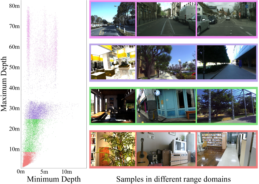
Figure 9: Range domain (RD) visualization. Different colors on the scatter plot represent images within different range domains.

A.2 Loss function of SM⁴Depth

Our network is supervised by multiple loss functions. As defined in the main paper, $\mathbf{D}$ represents the ground truth depth map, while $D$ signifies the predicted depth map. $D_{s}^{{}^{\prime}}$ denotes the depth map of the $s^{\text{th}}$ stage in the HSC-decoder. Additionally, $\mathbf{c}\in\mathbb{R}^{N\times 1}$ refers to the combined metric bin centers, and $y\in\mathbb{R}^{K\times 1}$ signifies the generated probabilities for $K$ RD. At the pixel level, we employ scale-invariant logarithmic (Silog) loss [15] to minimize per-pixel depth errors:

$$\!\!\mathcal{L}_{silog}(D,\mathbf{D})\!=\!\!\!\sqrt{\frac{1}{T}\!\!\sum_{i=1}^{T}\!\Big{(}\!\ln{\frac{D(i)}{\mathbf{D}(i)}}\Big{)}^{2}\!\!\!\!-\!\frac{\lambda}{T^{2}}\Big{(}\sum_{i=1}^{T}\!\ln{\frac{D(i)}{\mathbf{D}(i)}}\Big{)}^{2}}$$ (11)

where $T$ denotes the number of pixels with valid ground truth values, and we set $\lambda=0.85$. Then, we employ a multi-scale gradient matching term [34] to supervise the discontinuities between pixels in the depth map:

$$\mathcal{L}_{grad}(D,\mathbf{D})=\frac{1}{T}\sum_{m=1}^{M}\sum_{i=1}^{T}(|\nabla_{x}G_{i}^{m}|+|\nabla_{y}G_{i}^{m}|)$$ (12)

where $G_{i}=D(i)-\mathbf{D}(i)$. $G^{m}$ denotes the difference in disparity maps at scale $m$, and $M=4$ is the scale level. Overall, the pixel-wise loss function can be formulated as follows:

$$\mathcal{L}_{pixel}(D,\mathbf{D})=\alpha L_{silog}(D,\mathbf{D})+\beta L_{grad}(D,\mathbf{D})$$ (13)

where the coefficients $\alpha=10$ and $\beta=0.5$ are used in Eq.(13), learning the depth primarily and recovering the depth boundary secondarily. Then, the virtual normal loss [54] is employed to optimize the 3D structure:

$$\mathcal{L}_{vnl}(D,\mathbf{D})=\frac{1}{V}\sum_{i=1}^{V}(\parallel n_{i}-\mathbf{n}_{i}\parallel_{1})$$ (14)

where $V=0.15T$ is the sampling number of virtual planes. $n_{i}$ is the normal vector of the $i^{\text{th}}$ virtual plane in the output $D$ and $\mathbf{n}_{i}$ corresponds to the normal vector in $\mathbf{D}$.

Training Datasets	Scene	Capture	# Img	Range(m)
ScanNet [13]	Indoor	RGB-D	24,834	$[0,\ \ 10]$
Hypersim [37]	Indoor	Synthetic	15,229	$[0,\ \ 80]$
DIML Sample [10]	Indoor	RGB-D	1,609	$[0,\ \ \ \ 6]$
DIML Indoor [10]	Indoor	RGB-D	26,039	$[0,\ \ \ \ 8]$
DIML Outdoor [10]	Outdoor	Stereo*♯	24,031	$[0,\ \ 35]$
UASOL [2]	Outdoor	Stereo*♯	36,386	$[0,\ \ 35]$
ApolloScape [20]	Outdoor	LiDAR♯	14,908	$[0,\ \ 80]$
Cityscapes [12]	Outdoor	Stereo*♯	11,486	$[0,\ \ 80]$
total			154,522
Validation Datasets	Scene	Capture	# Img	Range(m)
NYUD [31]	Indoor	RGB-D	654	$[0,\ \ 10]$
KITTI [45]	Outdoor	LiDAR	652	$[0,\ \ 80]$
total			1,306
Test Datasets	Scene	Capture	# Img	Range(m)
SUN RGB-D [41]	Indoor	RGB-D	4,395	$[0,\ \ \ \ 8]$
iBims-1 [22]	Indoor	LiDAR	100	$[0,\ \ 50]$
ETH3D Indoor [38]	Indoor	LiDAR	219	$[0,\ \ 56]$
DIODE Indoor [46]	Indoor	LiDAR	325	$[0,\ \ 50]$
nuScenes-val [7]	Outdoor	LiDAR	1,138	$[0,140]$
DDAD [18]	Outdoor	LiDAR	3,950	$[0,\ \ 80]$
ETH3D Outdoor [38]	Outdoor	LiDAR	235	$[0,\ \ 73]$
DIODE Outdoor [46]	Outdoor	LiDAR	446	$[0,\ \ 80]$
BUPT Depth	Both-continuous	Stereo*♯	14,932	$[0,\ \ 30]$
total			25,740

Table 6: The metric depth datasets used in this paper. $*$ denotes the re-generation of metric depth by CREStereo [25], and ${\sharp}$ indicates the removal of sky regions in ground truth by ViT-Adapter [9].

At the scene level, the bi-directional Chamfer Loss [16] is employed to optimize the combination of bin centers $\mathbf{c}$, making them closer to the ground truth $\mathbf{D}$ as shown in Eq.(7) of the main paper: $\mathcal{L}_{bin}(\mathbf{c},\mathbf{D})$, with $N=256$ bins. Furthermore, the cross entropy loss is applied on the classification head (CLS):

$$\mathcal{L}_{cel}(y,\mathbf{y})=-\sum_{k=1}^{K}(\mathbf{y}_{k}\ln{y_{k}})$$ (15)

where $\mathbf{y}\in\mathbb{R}^{K\times 1}$ is the one-hot RD label of the input image.

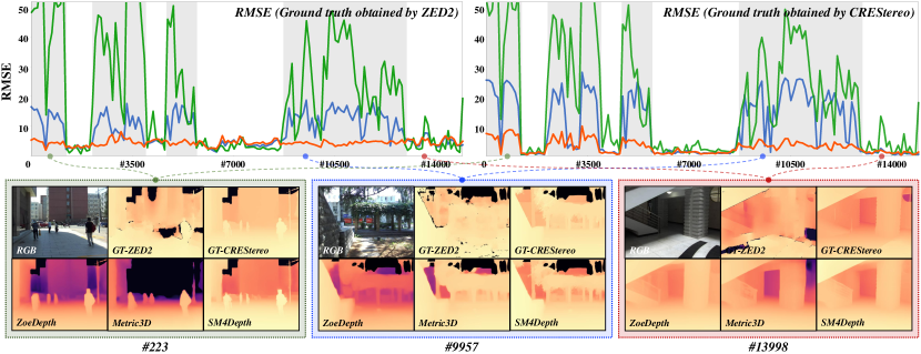
Figure 10: RMSE per frame of SM⁴Depth (red), Metirc3D (green) and ZoeDepth (blue) on BUPT Depth. We use the stereo depth of ZED2 (the first chart) and CREStereo[25] (the second chart) as ground truth, respectively. Gray indicates outdoor frames, and white indicates indoor frames.

Finally, the total loss of SM⁴Depth can be formulated as follows:

$$\begin{split}\mathcal{L}=\mathcal{L}_{pixel}(D,\mathbf{D})+\sum_{s=2}^{4}(\mathcal{L}_{pixel}(D^{{}^{\prime}}_{s},\mathbf{D}))+\\ \mu\mathcal{L}_{vnl}(D,\mathbf{D})+\gamma\mathcal{L}_{bin}(\mathbf{c},\mathbf{D})+\mathcal{L}_{cel}(y,\mathbf{y})\end{split}$$ (16)

where the coefficients $\mu$ and $\gamma$ are empirically set to $5$ and $0.1$ respectively.

Appendix B Appendix: Datasets Detail

Table 6 shows all datasets used for training, validation and testing. We conduct the same pre-processing operations before training as [5, 34].

Depth Re-generation: UASOL [2], CityScapes [12], and DIML [10] provide depth using a hand-crafted stereo matching method, which is not accurate enough. For this reason, we employ an advanced algorithm called CREStereo [25] to re-generate the ground truth.

Sky Removal: The images of outdoor datasets contain large areas of the sky, such as DIML, UASOL, ApolloScape, and CityScapes. We use ViT-Adapter [9] to extract sky areas and invalidate the depth values within these regions.

Appendix C Appendix: Results for Consistent Accuarcy

C.1 A seamless RGBD dataset: BUPT Depth

BUPT Depth (as shown in Fig. 11) is proposed to evaluate the consistency in accuracy across indoor and outdoor scenes, including streets, restaurants, classroom, lounges, etc. It consists of 14,932 continuous RGB-D pairs captured on the campus of the Beijing University of Posts and Telecommunications by a ZED2 stereo camera. In addition, we provide the re-generated depth maps from CREStereo [25] and the sky segmentations from ViT-Adapter [9]. The color and depth streams are captured with intrinsics of $1091.517$ and a baseline of $120.034\mathrm{mm}$.

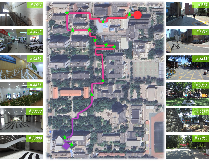
Figure 11: A top view of BUPT. This line represents the shooting route of the BUPT Depth dataset and several frames being visualized.

Method	Ground truth - ZED2
	$\mathbf{\delta_{1}\uparrow}$	$\mathbf{\delta_{2}\uparrow}$	$\mathbf{\delta_{3}\uparrow}$	REL$\downarrow$	RMSE$\downarrow$	log10$\downarrow$
ZoeD-NK	0.314	0.485	0.576	1.006	9.758	0.263
Metric3D	0.155	0.318	0.417	2.446	23.794	0.427
SM4Depth	0.536	0.805	0.924	0.295	3.440	0.118
Method	Ground truth - CREStereo
	$\mathbf{\delta_{1}\uparrow}$	$\mathbf{\delta_{2}\uparrow}$	$\mathbf{\delta_{3}\uparrow}$	REL$\downarrow$	RMSE$\downarrow$	log10$\downarrow$
ZoeD-NK	0.365	0.505	0.579	0.974	9.377	0.252
Metric3D	0.293	0.402	0.470	1.816	22.736	0.352
SM4Depth	0.629	0.875	0.966	0.241	2.888	0.094

Table 7: Quantitative results on BUPT Depth. Comparisons are conducted with the ground truths of ZED and CREStereo, respectively. The best results are in bold, and the second-best ones are underlined.

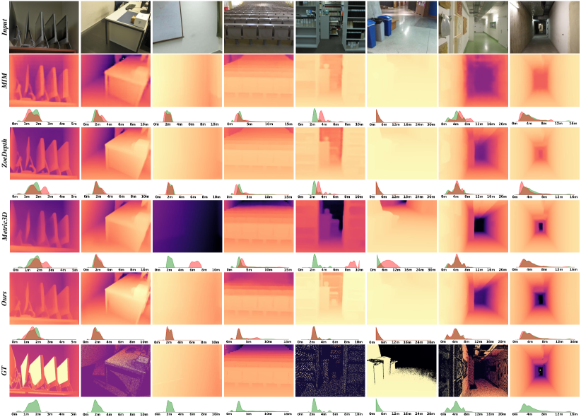
Figure 12: Qualitative results in indoor scenes. The depth distribution is under the depth maps with green for ground truth and red for prediction. Our method performs better on images with multiple viewpoints and diverse scenes.

C.2 Quantitative result on BUPT Depth

Table 7 illustrates the quantitative comparison between ZoeD-NK, Metric3D, and SM⁴Depth with the ground truth obtained from ZED2 and CREStereo [25]. It can be seen that SM⁴Depth outperforms ZoeDepth and Metric3D across all metrics, whether using ground truth ZED2 or ground truth CREStereo.

C.3 Qualitative result on BUPT Depth

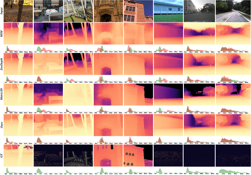
Figure 13: Qualitative results in outdoor scenes. The depth distribution is under the depth maps with green for ground truth and red for prediction. Our method performs better on images with multiple viewpoints and diverse scenes.

To compare ZoeDepth, Metric3D, and SM⁴Depth temporally, we visualize the RMSE of each frame by a line chart (see Fig. 10). It can be observed that ZoeDepth (blue line) and Metric3D (green line) exhibit significantly larger fluctuations than that of SM⁴Depth (red line). No matter using which ground truth, both methods achieve good performance in indoor scenes. However, ZoeD-NK obtains RMSEs higher than 10 in almost all outdoor scenes, and the RMSEs of Metric3D are even higher than 20, while SM⁴Depth still achieves equal RMSEs in both indoor and outdoor scenes. And SM⁴Depth can recover more depth details due to its refinement structure of the HSC-Decoder.

Appendix D Appendix: Additional Comparison

To demonstrate the superiority of our method thoroughly, we append more qualitative comparisons in Fig. 12 (indoor scenes) and Fig. 13 (outdoor scenes). SM⁴Depth obtains a more accurate metric scale and depth range than other methods, with almost no shift in depth distribution.

References

- Anthes et al. [2016] Christoph Anthes, Rubén Jesús García-Hernández, Markus Wiedemann, and Dieter Kranzlmüller. State of the art of virtual reality technology. In IEEE Aerospace Conference, pages 1–19, 2016.
- Bauer et al. [2019] Zuria Bauer, Francisco Gomez-Donoso, Edmanuel Cruz, Sergio Orts-Escolano, and Miguel Cazorla. Uasol, a large-scale high-resolution outdoor stereo dataset. Scientific data, 6(1):162, 2019.
- Bhat et al. [2021] Shariq Farooq Bhat, Ibraheem Alhashim, and Peter Wonka. Adabins: Depth estimation using adaptive bins. In IEEE Conference on Computer Vision and Pattern Recognition (CVPR), 2021.
- Bhat et al. [2022] Shariq Farooq Bhat, Ibraheem Alhashim, and Peter Wonka. Localbins: Improving depth estimation by learning local distributions. In Computer Vision–ECCV 2022: 17th European Conference, Tel Aviv, Israel, October 23–27, 2022, Proceedings, Part I, pages 480–496. Springer, 2022.
- Bhat et al. [2023] Shariq Farooq Bhat, Reiner Birkl, Diana Wofk, Peter Wonka, and Matthias Müller. Zoedepth: Zero-shot transfer by combining relative and metric depth, 2023.
- Braun et al. [2022] Daniel Braun, Olivier Morell, Pascal Vasseur, and Cédric Demonceaux. N-qgn: Navigation map from a monocular camera using quadtree generating networks. In International Conference on Robotics and Automation (ICRA), 2022.
- Caesar et al. [2020] Holger Caesar, Varun Bankiti, Alex H Lang, Sourabh Vora, Venice Erin Liong, Qiang Xu, Anush Krishnan, Yu Pan, Giancarlo Baldan, and Oscar Beijbom. nuscenes: A multimodal dataset for autonomous driving. In Proceedings of the IEEE/CVF conference on computer vision and pattern recognition, pages 11621–11631, 2020.
- Chen et al. [2019] Xiaotian Chen, Xuejin Chen, and Zheng-Jun Zha. Structure-aware residual pyramid network for monocular depth estimation. In International Joint Conference on Artificial Intelligence (IJCAI), 2019.
- Chen et al. [2022] Zhe Chen, Yuchen Duan, Wenhai Wang, Junjun He, Tong Lu, Jifeng Dai, and Yu Qiao. Vision transformer adapter for dense predictions. arXiv preprint arXiv:2205.08534, 2022.
- Cho et al. [2021] Jaehoon Cho, Dongbo Min, Youngjung Kim, and Kwanghoon Sohn. DIML/CVL RGB-D dataset: 2m rgb-d images of natural indoor and outdoor scenes. arXiv preprint arXiv:2110.11590, 2021.
- Chu and Hsu [2018] Wei-Ta Chu and Yu-Ting Hsu. Depth-aware image colorization network. In ACMMM Workshop, 2018.
- Cordts et al. [2016] Marius Cordts, Mohamed Omran, Sebastian Ramos, Timo Rehfeld, Markus Enzweiler, Rodrigo Benenson, Uwe Franke, Stefan Roth, and Bernt Schiele. The cityscapes dataset for semantic urban scene understanding. In Proc. of the IEEE Conference on Computer Vision and Pattern Recognition (CVPR), 2016.
- Dai et al. [2017] Angela Dai, Angel X. Chang, Manolis Savva, Maciej Halber, Thomas Funkhouser, and Matthias Nießner. Scannet: Richly-annotated 3d reconstructions of indoor scenes. In Proc. Computer Vision and Pattern Recognition (CVPR), IEEE, 2017.
- Eigen and Fergus [2015] David Eigen and Rob Fergus. Predicting depth, surface normals and semantic labels with a common multi-scale convolutional architecture. In IEEE International Conference on Computer Vision (ICCV), 2015.
- Eigen et al. [2014] David Eigen, Christian Puhrsch, and Rob Fergus. Depth map prediction from a single image using a multi-scale deep network. In Neural Information Processing Systems (NIPS), 2014.
- Fan et al. [2017] Haoqiang Fan, Hao Su, and Leonidas Guibas. A point set generation network for 3d object reconstruction from a single image. In 2017 IEEE Conference on Computer Vision and Pattern Recognition (CVPR), 2017.
- Fu et al. [2018] Huan Fu, Mingming Gong, Chaohui Wang, Kayhan Batmanghelich, and Dacheng Tao. Deep ordinal regression network for monocular depth estimation. In IEEE Conference on Computer Vision and Pattern Recognition (CVPR), 2018.
- Guizilini et al. [2020] Vitor Guizilini, Rares Ambrus, Sudeep Pillai, Allan Raventos, and Adrien Gaidon. 3d packing for self-supervised monocular depth estimation. In IEEE Conference on Computer Vision and Pattern Recognition (CVPR), 2020.
- Huang et al. [2022] Kuan-Chih Huang, Tsung-Han Wu, Hung-Ting Su, and Winston H. Hsu. Monodtr: Monocular 3d object detection with depth-aware transformer. In IEEE/CVF Conference on Computer Vision and Pattern Recognition (CVPR), 2022.
- Huang et al. [2018] Xinyu Huang, Xinjing Cheng, Qichuan Geng, Binbin Cao, Dingfu Zhou, Peng Wang, Yuanqing Lin, and Ruigang Yang. The apolloscape dataset for autonomous driving. In Proceedings of the IEEE conference on computer vision and pattern recognition workshops, pages 954–960, 2018.
- Ioannou and Maddock [2022] Eleftherios Ioannou and Steve Maddock. Depth-aware neural style transfer using instance normalization. In Computer Graphics & Visual Computing (CGVC) 2022. Eurographics Digital Library, 2022.
- Koch et al. [2018] Tobias Koch, Lukas Liebel, Friedrich Fraundorfer, and Marco Korner. Evaluation of cnn-based single-image depth estimation methods. In Proceedings of the European Conference on Computer Vision (ECCV) Workshops, pages 0–0, 2018.
- Laina et al. [2016] Iro Laina, Christian Rupprecht, Vasileios Belagiannis, Federico Tombari, and Nassir Navab. Deeper depth prediction with fully convolutional residual networks. In International Conference on 3D Vision (3DV), 2016.
- Lee et al. [2019] Jin Han Lee, Myung-Kyu Han, Dong Wook Ko, and Il Hong Suh. From big to small: Multi-scale local planar guidance for monocular depth estimation. arXiv preprint arXiv:1907.10326, 2019.
- Li et al. [2022a] Jiankun Li, Peisen Wang, Pengfei Xiong, Tao Cai, Ziwei Yan, Lei Yang, Jiangyu Liu, Haoqiang Fan, and Shuaicheng Liu. Practical stereo matching via cascaded recurrent network with adaptive correlation. In Proceedings of the IEEE/CVF Conference on Computer Vision and Pattern Recognition, pages 16263–16272, 2022a.
- Li and Snavely [2018] Zhengqi Li and Noah Snavely. Megadepth: Learning single-view depth prediction from internet photos. In Proceedings of the IEEE conference on computer vision and pattern recognition, pages 2041–2050, 2018.
- Li et al. [2022b] Zhenyu Li, Xuyang Wang, Xianming Liu, and Junjun Jiang. Binsformer: Revisiting adaptive bins for monocular depth estimation. arXiv preprint arXiv:2204.00987, 2022b.
- Liu et al. [2019] Chao Liu, Jinwei Gu, Kihwan Kim, Srinivasa G Narasimhan, and Jan Kautz. Neural rgb (r) d sensing: Depth and uncertainty from a video camera. In IEEE/CVF Conference on Computer Vision and Pattern Recognition (CVPR), 2019.
- Liu et al. [2017] Xiao-Chang Liu, Ming-Ming Cheng, Yu-Kun Lai, and Paul L Rosin. Depth-aware neural style transfer. In Proceedings of the symposium on non-photorealistic animation and rendering, 2017.
- Lu et al. [2019] Shufang Lu, Wei Jiang, Xuefeng Ding, Craig S. Kaplan, Xiaogang Jin, Fei Gao, and Jiazhou Chen. Depth-aware image vectorization and editing. The Visual Computer, 35(6):1027–1039, 2019.
- Nathan Silberman and Fergus [2012] Pushmeet Kohli Nathan Silberman, Derek Hoiem and Rob Fergus. Indoor segmentation and support inference from rgbd images. In ECCV, 2012.
- ng et al. [2020] Mingyu ng, Yuqi Huo, Hongwei Yi, Zhe Wang, Jianping Shi, Zhiwu Lu, and Ping Luo. Learning depth-guided convolutions for monocular 3d object detection. In IEEE/CVF Conference on Computer Vision and Pattern Recognition Workshops (CVPRW), 2020.
- Nie et al. [2017] Bruce Xiaohan Nie, Ping Wei, and Song-Chun Zhu. Monocular 3d human pose estimation by predicting depth on joints. In IEEE International Conference on Computer Vision (ICCV), 2017.
- Ranftl et al. [2020] René Ranftl, Katrin Lasinger, David Hafner, Konrad Schindler, and Vladlen Koltun. Towards robust monocular depth estimation: Mixing datasets for zero-shot cross-dataset transfer. IEEE transactions on pattern analysis and machine intelligence, 44(3):1623–1637, 2020.
- Ranftl et al. [2021a] René Ranftl, Alexey Bochkovskiy, and Vladlen Koltun. Vision transformers for dense prediction. In Proceedings of the IEEE/CVF International Conference on Computer Vision, pages 12179–12188, 2021a.
- Ranftl et al. [2021b] René Ranftl, Alexey Bochkovskiy, and Vladlen Koltun. Vision transformers for dense prediction. In Proceedings of the IEEE/CVF International Conference on Computer Vision, pages 12179–12188, 2021b.
- Roberts et al. [2021] Mike Roberts, Jason Ramapuram, Anurag Ranjan, Atulit Kumar, Miguel Angel Bautista, Nathan Paczan, Russ Webb, and Joshua M. Susskind. Hypersim: A photorealistic synthetic dataset for holistic indoor scene understanding. In International Conference on Computer Vision (ICCV) 2021, 2021.
- Schöps et al. [2017a] Thomas Schöps, Johannes L. Schönberger, Silvano Galliani, Torsten Sattler, Konrad Schindler, Marc Pollefeys, and Andreas Geiger. A multi-view stereo benchmark with high-resolution images and multi-camera videos. In Conference on Computer Vision and Pattern Recognition (CVPR), 2017a.
- Schöps et al. [2017b] Thomas Schöps, Johannes L. Schönberger, Silvano Galliani, Torsten Sattler, Konrad Schindler, Marc Pollefeys, and Andreas Geiger. A multi-view stereo benchmark with high-resolution images and multi-camera videos. In IEEE Conference on Computer Vision and Pattern Recognition (CVPR), 2017b.
- Sheng et al. [2022] Fei Sheng, Feng Xue, Yicong Chang, Wenteng Liang, and Anlong Ming. Monocular depth distribution alignment with low computation. In International Conference on Robotics and Automation (ICRA), 2022.
- Song et al. [2015] Shuran Song, Samuel P Lichtenberg, and Jianxiong Xiao. SUN RGB-D: A rgb-d scene understanding benchmark suite. In Proceedings of the IEEE conference on computer vision and pattern recognition, pages 567–576, 2015.
- Sun et al. [2021] Li Sun, Marwan Taher, Christopher Wild, Cheng Zhao, Yu Zhang, Filip Majer, Zhi Yan, Tomáš Krajník, Tony Prescott, and Tom Duckett. Robust and long-term monocular teach and repeat navigation using a single-experience map. In IEEE/RSJ International Conference on Intelligent Robots and Systems (IROS), 2021.
- Sun et al. [2022] Yu Sun, Wu Liu, Qian Bao, Yili Fu, Tao Mei, and Michael J Black. Putting people in their place: Monocular regression of 3d people in depth. In Proceedings of the IEEE/CVF Conference on Computer Vision and Pattern Recognition, 2022.
- Tateno et al. [2017] K. Tateno, F. Tombari, I. Laina, and N. Navab. CNN-SLAM: Real-time dense monocular slam with learned depth prediction. In IEEE Conference on Computer Vision and Pattern Recognition (CVPR), 2017.
- Uhrig et al. [2017] Jonas Uhrig, Nick Schneider, Lukas Schneider, Uwe Franke, Thomas Brox, and Andreas Geiger. Sparsity invariant cnns. In International Conference on 3D Vision (3DV), 2017.
- Vasiljevic et al. [2019] Igor Vasiljevic, Nick Kolkin, Shanyi Zhang, Ruotian Luo, Haochen Wang, Falcon Z. Dai, Andrea F. Daniele, Mohammadreza Mostajabi, Steven Basart, Matthew R. Walter, and Gregory Shakhnarovich. DIODE: A Dense Indoor and Outdoor DEpth Dataset. CoRR, abs/1908.00463, 2019.
- Wang and Shen [2018] Kaixuan Wang and Shaojie Shen. Mvdepthnet: Real-time multiview depth estimation neural network. In International Conference on 3D Vision (3DV), 2018.
- Xie et al. [2022] Zhenda Xie, Zigang Geng, Jingcheng Hu, Zheng Zhang, Han Hu, and Yue Cao. Revealing the dark secrets of masked image modeling. arXiv preprint arXiv:2205.13543, 2022.
- Xue et al. [2019] F. Xue, A. Ming, M. Zhou, and Y. Zhou. A novel multi-layer framework for tiny obstacle discovery. In IEEE International Conference on Robotics and Automation (ICRA), 2019.
- Xue et al. [2020] F. Xue, A. Ming, and Y. Zhou. Tiny obstacle discovery by occlusion-aware multilayer regression. IEEE Transactions on Image Processing (TIP), 29:9373–9386, 2020.
- Xue et al. [2021] Feng Xue, Junfeng Cao, Yu Zhou, Fei Sheng, Yankai Wang, and Anlong Ming. Boundary-induced and scene-aggregated network for monocular depth prediction. Pattern Recognition (PR), 115:107901, 2021.
- Xue et al. [2022] Fei Xue, Xin Wang, Junqiu Wang, and Hongbin Zha. Deep visual odometry with adaptive memory. IEEE Transactions on Pattern Analysis and Machine Intelligence, 44(2):940–954, 2022.
- Xue et al. [2023] Feng Xue, Yicong Chang, Tianxi Wang, Yu Zhou, and Anlong Ming. Indoor Obstacle Discovery on Reflective Ground via Monocular Camera. International Journal of Computer Vision, 2023.
- Yin et al. [2019] Wei Yin, Yifan Liu, Chunhua Shen, and Youliang Yan. Enforcing geometric constraints of virtual normal for depth prediction. In Proceedings of the IEEE/CVF International Conference on Computer Vision, pages 5684–5693, 2019.
- Yin et al. [2022] Wei Yin, Jianming Zhang, Oliver Wang, Simon Niklaus, Simon Chen, Yifan Liu, and Chunhua Shen. Towards accurate reconstruction of 3d scene shape from a single monocular image. IEEE Transactions on Pattern Analysis and Machine Intelligence, 2022.
- Yin et al. [2023] Wei Yin, Chi Zhang, Hao Chen, Zhipeng Cai, Gang Yu, Kaixuan Wang, Xiaozhi Chen, and Chunhua Shen. Metric3d: Towards zero-shot metric 3d prediction from a single image. In IEEE International Conference on Computer Vision (ICCV), 2023.
- Yuan et al. [2022] Weihao Yuan, Xiaodong Gu, Zuozhuo Dai, Siyu Zhu, and Ping Tan. New crfs: Neural window fully-connected crfs for monocular depth estimation. arXiv preprint arXiv:2203.01502, 2022.
- Zhang et al. [2022] Sen Zhang, Jing Zhang, and Dacheng Tao. Towards scale consistent monocular visual odometry by learning from the virtual world. In International Conference on Robotics and Automation (ICRA), 2022.
- Zhenda et al. [2023] Xie Zhenda, Geng Zigang, Hu Jingcheng, Zhang Zheng, Hu Han, and Cao Yue. Revealing the dark secrets of masked image modeling. In IEEE Conference on Computer Vision and Pattern Recognition (CVPR), 2023.