Regret Analysis of Policy Optimization over Submanifolds
for Linearly Constrained Online LQG

Ting-Jui Chang and Shahin Shahrampour, Senior Member, IEEE T.J. Chang and S. Shahrampour are with the Department of Mechanical and Industrial Engineering, Northeastern University, Boston, MA 02115, USA. email:{chang.tin,s.shahrampour}@northeastern.edu.
Abstract

Recent advancement in online optimization and control has provided novel tools to study online linear quadratic regulator (LQR) problems, where cost matrices are varying adversarially over time. However, the controller parameterization of existing works may not satisfy practical conditions like sparsity due to physical connections. In this work, we study online linear quadratic Gaussian problems with a given linear constraint imposed on the controller. Inspired by the recent work of [1] which proposed, for a linearly constrained policy optimization of an offline LQR, a second order method equipped with a Riemannian metric that emerges naturally in the context of optimal control problems, we propose online optimistic Newton on manifold (OONM) which provides an online controller based on the prediction on the first and second order information of the function sequence. To quantify the proposed algorithm, we leverage the notion of regret defined as the sub-optimality of its cumulative cost to that of a (locally) minimizing controller sequence and provide the regret bound in terms of the path-length of the minimizer sequence. Simulation results are also provided to verify the property of OONM.

I Introduction

Linear quadratic regulator (LQR) is one of the most widely studied optimal control problems in control theory ([2]), and it has been applied to problems in different fields such as econometrics, robotics and physics. It is also well known that if the governing dynamics and the cost matrices are known, the optimal controller can be derived by solving the Riccati equations.

However, this well-structured property can not accommodate the need of some practical LQR problems, especially for those lie in non-stationary environments since the cost parameters may change adversarially over time and are unknown in advance to the learner. To tackle online LQR problem of this kind, different approaches were proposed to reformulate online control problems as online optimization problem (e.g., semidefinite programming (SDP) relaxation for time-varying LQR [3] and noise feedback policy design for time-varying convex costs with adversarial noises in [4]), and techniques from online learning literature were applied to generate an adaptive controller in real time. As problems in online optimization, the performance of an online control algorithm is gauged by regret, which is defined as the sub-optimality of the cumulative cost incurred by the algorithm to that of a given comparator policy.

Despite enjoyable performance guarantees, in those existing works of online control ([3, 4, 5, 6, 7]), the online controller is typically parameterized as a linear function of the state or past noises, where the coefficient matrices are likely to be dense so that the controller formulation can not satisfy some practical conditions such as the sparsity requirement. For offline LQR problems, the linearly constrained setup was recently studied in [1], where the authors proposed a second order method where the Hessian operator is defined based on a Riemannian metric arising from the optimal control problem itself. In this work, we further extend the idea to the online setup, aiming at providing an adaptive control satisfying the physical constraint in real time. The contribution of this work can be summarized as follows

  • โ€ข

    Inspired by [1], for linearly constrained online LQG problems, we propose OONM, which is a Riemannian metric based second order approach where the predictions on the cost functions are used during the learning process.

  • โ€ข

    Instead of being compared to a fixed control policy, we focus on the regret defined against a sequence of (locally) minimizing linear policies, and we present the dynamic regret bound in terms of the path length of the minimizer sequence and the prediction mismatch.

II Related Works

Policy Optimization of LQR: For offline LQR problems, the convergence property of gradient-based method has been studied for both discrete-time and continuous-time cases [8, 9, 10, 11], where the LQR costs are shown to satisfy the gradient dominance property which ensure fast convergence though the cost is not convex. However, for general constrained LQR problems, this property does not necessarily hold and gradienct-based methods like Projected Gradient Descent (PGD) are shown with a sub-linear convergence rate to first order stationary points [9]. Recently, the authors of [1] proposed a second order update method for linearly constrained LQR where the Hessian operator is defined based on the Riemannian metric coming from the optimization objective, and the convergence rate was shown to be locally linear-quadratic.
Online Optimization: The field of online learning has been well-studied and there is a rich body of literature. The general goal of the learner is to make the decision sequence in an online fashion without knowing in advance the function sequence which can change adversarially. As mentioned earlier, the performance of an online algorithm is captured by the idea of regret, which is considered to be static (dynamic) if the comparator decision is fixed (changing) over time. For the static case, it is well known that the optimal regret bounds are $O(\sqrt{T})$ and $O\left(\log(T)\right)$ for convex and strongly-convex functions, respectively [12, 13]. For the dynamic case, as the function sequence varies in an arbitrarily manner, typically there is no explicitly sub-linear regret bound. Instead, the dynamic regret bound is presented in terms of different regularity measures of the comparator sequence: path-length [12, 14, 15], function value variation [16], variation in gradients or Hessians [17, 18, 19, 20].
Online Control: The recent advancement in online optimization and control has fueled the interesting in studying linear dynamical systems with time-varying costs. For linear time-invariant (LTI) systems known dynamics, [3] reformulated the online LQG problem with SDP relaxation and established a regret bound of $O(\sqrt{T})$. The setup was later extended to the case with general convex functions and adversarial noises in [4], where the disturbance-action controller (DAC) parameterization was proposed and a regret bound of $O(\sqrt{T})$ was derived. The regret bound was later improved to $O\left(\text{poly}(\log(T))\right)$ in [5] when strongly-convex functions were considered. Besides the case with known linear dynamics, the setup with unknown dynamics was also studied for convex costs [21] and strongly-convex costs [6]. For dynamic regret bounds, [22] studied the setup with general convex costs for a LTI systems and derived the dynamic regret bound with respect to a time-varying DAC. This bound was later improved when the costs were quadratic [23]. A different setup with linear time-varying systems was studied and the corresponding dynamic bound was proposed in [24]. Motivated by the safety concern, the setup where constraints are imposed on states and controls was also studied in the literature [25, 26].

III Problem Formulation

III-A Notation

$\rho(\mathbf{A})$ The spectral radius of matrix $\mathbf{A}$
$\left\lVert\cdot\right\rVert$ Euclidean (spectral) norm of a vector (matrix)
$\left\lVert\cdot\right\rVert_{g}$ Norm defined based on a Riemannian metric $g$
$\text{dist}(\cdot,\cdot)$ Riemannian distance based on metric $g$
$\mathbb{E}[\cdot]$ The expectation operator
$\mathbb{L}(\mathbf{A},\mathbf{Z})$ Lyapunov map to $\mathbf{X}:\mathbf{X}=\mathbf{A}\mathbf{X}\mathbf{A}^{\top}+\mathbf{Z}$
$\mathbf{I}_{d}$ Identity matrix with dimension $d\times d$

III-B Linearly Constrained Online LQG Control

We consider a fully-observable LTI system with the following dynamics

$$\mathbf{x}_{t+1}=\mathbf{A}\mathbf{x}_{t}+\mathbf{B}\mathbf{u}_{t}+\mathbf{w}_{t},$$

where the system matrices $\mathbf{A}\in\mathrm{R}^{n\times n}$ and $\mathbf{B}\in\mathrm{R}^{n\times m}$ are known to the learner, and $\mathbf{w}_{t}$ is a Gaussian noise with zero mean and covariance $\mathbf{W}\succeq\sigma^{2}\mathbf{I}$. The noise sequence $\{\mathbf{w}_{t}\}$ is assumed to be independent and identical over time. The general goal of an online LQG problem is that given a sequence of cost matrices pair $\{(\mathbf{Q}_{t},\mathbf{R}_{t})\}$ which is unknown in advance and revealed to the learner in a sequential manner, the learner needs to decides the control signal in a real time sense while ensuring an acceptable cumulative cost. In other words, at round $t$, the learner receives the state $\mathbf{x}_{t}$ and applies the control $\mathbf{u}_{t}$. Then, positive definite cost matrices $\mathbf{Q}_{t}$ and $\mathbf{R}_{t}$ are revealed, and the cost $\mathbf{x}_{t}^{\top}\mathbf{Q}_{t}\mathbf{x}_{t}+\mathbf{u}_{t}^{\top}\mathbf{R}_{t}\mathbf{u}_{t}$ is incurred.
Linearly Constrained Controllers: In existing literature regarding online control on a LTI system, the control $\mathbf{u}_{t}$ is parameterized as a linear function of the past states $\{\mathbf{x}_{i}\}_{i\leq t}$. However, this parameterization normally comes with dense coefficient matrices which may not satisfies practical conditions, e.g., the sparsity requirement due to physical connections. As opposed to previous studies, in this work, we seek to learn a sequence of linear controllers $\{\mathbf{K}_{t}\}$ $(\mathbf{u}_{t}=\mathbf{K}_{t}\mathbf{x}_{t})$ which satisfies a given linear constraint.
Regret Definition: To quantify the performance of an online LQG control algorithm $\mathcal{A}$, we focus on its finite-time sub-optimality with respect to a comparator policy $\pi$ which induces the cumulative cost after $T$ steps as follows

$$J_{T}(\pi)=\mathrm{E}\left[\sum_{t=1}^{T}{\mathbf{x}_{t}^{\pi}}^{\top}\mathbf{Q}_{t}\mathbf{x}_{t}^{\pi}+{\mathbf{u}_{t}^{\pi}}^{\top}\mathbf{R}_{t}\mathbf{u}_{t}^{\pi}\right].$$ (1)

In this work, the selected comparator policy $\pi$ is also parameterized as a sequence of linear controllers $\{\mathbf{K}^{*}_{t}\}$ where $\mathbf{K}^{*}_{t}$ is, under the given linear constraint, an (local) minimizer of the infinite time-horizon LQG problem with $(\mathbf{Q}_{t},\mathbf{R}_{t})$ as the corresponding cost matrices. Note that this comparator policy is greedy in a sense that if the cost matrices pair stays constant after step $t$, then the policy $\mathbf{u}=\mathbf{K}^{*}_{t}\mathbf{x}_{t}$ enjoys the (locally) optimal performance when $T$ goes to infinity. Based on Equation (1), the regret (finite-time sub-optimality) of an online algorithm $\mathcal{A}$ is defined as follows

$$\text{Regret}_{T}(\mathcal{A}):=J_{T}(\mathcal{A})-J_{T}(\pi),$$ (2)

where $J_{T}(\mathcal{A})=\mathrm{E}\left[\sum_{t=1}^{T}{\mathbf{x}_{t}^{\mathcal{A}}}^{\top}\mathbf{Q}_{t}\mathbf{x}_{t}^{\mathcal{A}}+{\mathbf{u}_{t}^{\mathcal{A}}}^{\top}\mathbf{R}_{t}\mathbf{u}_{t}^{\mathcal{A}}\right]$.

III-C Strong Stability and Sequential Strong Stability

In order to quantify the convergence rate of a stable controller, following cohen, we also introduce the notion of strong stability.

Definition 1

(Strong Stability) A linear policy $\mathbf{K}$ is $(\kappa,\gamma)$-strongly stable (for $\kappa>0$ and $0<\gamma\leq 1$) for the LTI system $(\mathbf{A},\mathbf{B})$, if $\left\lVert\mathbf{K}\right\rVert\leq\kappa$, and there exist matrices $\mathbf{L}$ and $\mathbf{H}$ such that $\mathbf{A}+\mathbf{B}\mathbf{K}=\mathbf{H}\mathbf{L}\mathbf{H}^{-1}$, with $\left\lVert\mathbf{L}\right\rVert\leq 1-\gamma$ and $\left\lVert\mathbf{H}\right\rVert\|\mathbf{H}^{-1}\|\leq\kappa$.

Note that the idea of strong stability simply provides a quantitative perspective viewing a stable controller. In fact, any stable controller can shown to be strongly stable for some $\kappa$ and $\gamma$ cohen. And on the top of strong stability, we can easily quantify the rate of convergence to the steady state distribution. Besides strong stability, as the applied controller $\mathbf{K}_{t}$ is changing over time in the online setup, we introduce another notion of strong stability defined in cohen:

Definition 2

(Sequential Strong Stability) A sequence of linear policies $\{\mathbf{K}_{t}\}_{t=1}^{T}$ is $(\kappa,\gamma)$-strongly stable if there exist matrices $\{\mathbf{H}_{t}\}_{t=1}^{T}$ and $\{\mathbf{L}_{t}\}_{t=1}^{T}$ such that $\mathbf{A}+\mathbf{B}\mathbf{K}_{t}=\mathbf{H}_{t}\mathbf{L}_{t}\mathbf{H}_{t}^{-1}$ for all $t$ with the following properties,

  1. 1.

    $\left\lVert\mathbf{L}_{t}\right\rVert\leq 1-\gamma$ and $\left\lVert\mathbf{K}_{t}\right\rVert\leq\kappa$.

  2. 2.

    $\left\lVert\mathbf{H}_{t}\right\rVert\leq\beta^{\prime}$ and $\left\lVert\mathbf{H}_{t}^{-1}\right\rVert\leq 1/\alpha^{\prime}$ with $\kappa=\beta^{\prime}/\alpha^{\prime}$.

  3. 3.

    $\left\lVert\mathbf{H}_{t+1}^{-1}\mathbf{H}_{t}\right\rVert\leq 1+\gamma/2$.

And the corresponding convergence to the steady-state covariance matrices induced by $\{\mathbf{K}_{t}\}$ is characterized as follows.

Lemma 1

(Lemma 3.5 in [3]) Suppose a time-varying policy ($\mathbf{u}_{t}=\mathbf{K}_{t}\mathbf{x}_{t}$) is applied. Denote the steady-state covariance matrix of $\mathbf{K}_{t}$ as ๐—tssubscriptsuperscript๐—๐‘ ๐‘ก\mathbf{X}^{s}_{t}. If $\{\mathbf{K}_{t}\}$ are $(\kappa,\gamma)$-sequentially strongly stable and โˆฅ๐—tsโˆ’๐—tโˆ’1sโˆฅโ‰คฮทdelimited-โˆฅโˆฅsubscriptsuperscript๐—๐‘ ๐‘กsubscriptsuperscript๐—๐‘ ๐‘ก1๐œ‚\left\lVert\mathbf{X}^{s}_{t}-\mathbf{X}^{s}_{t-1}\right\rVert\leq\eta, $\mathbf{X}_{t}$ (the state covariance matrix of $\mathbf{x}_{t}$) converges to ๐—tssubscriptsuperscript๐—๐‘ ๐‘ก\mathbf{X}^{s}_{t} as follows

โˆฅ๐—t+1โˆ’๐—t+1sโˆฅโ‰คฮบ2โ€‹eโˆ’ฮณโ€‹tโ€‹โˆฅ๐—1โˆ’๐—1sโˆฅ+2โ€‹ฮทโ€‹ฮบ2ฮณ.delimited-โˆฅโˆฅsubscript๐—๐‘ก1subscriptsuperscript๐—๐‘ ๐‘ก1superscript๐œ…2superscript๐‘’๐›พ๐‘กdelimited-โˆฅโˆฅsubscript๐—1subscriptsuperscript๐—๐‘ 12๐œ‚superscript๐œ…2๐›พ\left\lVert\mathbf{X}_{t+1}-\mathbf{X}^{s}_{t+1}\right\rVert\leq\kappa^{2}e^{-\gamma t}\left\lVert\mathbf{X}_{1}-\mathbf{X}^{s}_{1}\right\rVert+\frac{2\eta\kappa^{2}}{\gamma}.

III-D Policy Optimization over Manifold for Static LQ Control

For a stabilizable pair $(\mathbf{A},\mathbf{B})$, we define the set of stable linear controllers as follows

$$\mathcal{S}:=\{\mathbf{K}\in\mathrm{R}^{m\times n}\;|\;\rho(\mathbf{A}+\mathbf{B}\mathbf{K})<1\}.$$

In the work of Shariar, the authors showed that if a static LQR problem is formulated as a optimization problem over manifold equipped with the Riemannian metric arising from the original problem, the learning process can better capture the inherent geometry, which in turns provides a more precise update direction.
Problem-oriented Riemannian Metric: In this work, we consider $\mathcal{S}$ as a manifold on its own, then we define the following notations: $T\mathcal{S}$ denotes the the tangent bundle of $\mathcal{S}$; $T_{\mathbf{K}}\mathcal{S}$ denotes the tangent space at a point $\mathbf{K}\in\mathcal{S}$; A vector field $V$ on $\mathcal{S}$ is a smooth map $V\;:\;\mathcal{S}\mapsto T\mathcal{S}$ such that $V_{\mathbf{K}}\in T_{\mathbf{K}}\mathcal{S}$ for all $\mathbf{K}\in\mathcal{S}$, and $\mathfrak{X}(\mathcal{S})$ denotes the set of all vector fields over $\mathcal{S}$; A covariant 2-tensor field is a smooth real-valued multilinear function of two vector fields, and the bundle of covariant 2-tensor fields is denoted as $T^{2}(T^{*}\mathcal{S})$.

Note that infinite-horizon LQR control problems and Linear Quadratic Gaussian (LQG) share a similar cost formulation: $f(\mathbf{K})=\text{Tr}(\mathbf{P}_{\mathbf{K}}\Sigma_{\mathbf{K}})$ where functions $\mathbf{P},\Sigma:\mathcal{S}\mapsto\mathrm{R}^{n\times n}$ map $\mathbf{K}$ to

$$\begin{split}\mathbf{P}_{\mathbf{K}}&:=\mathbb{L}\big{(}(\mathbf{A}+\mathbf{B}\mathbf{K})^{\top},\mathbf{Q}+\mathbf{K}^{\top}\mathbf{R}\mathbf{K}\big{)},\\ \Sigma_{\mathbf{K}}&:=\Sigma_{1}+\mathbf{K}^{\top}\Sigma_{2}\mathbf{K},\end{split}$$ (3)

respectively, and $\Sigma_{1},\Sigma_{2}\succeq 0$ are prescribed matrices. Then based on the Lyapunov-trace property, the cost can be reformulated as $f(\mathbf{K})=\text{Tr}\left((\mathbf{Q}+\mathbf{K}^{\top}\mathbf{R}\mathbf{K})\mathbb{L}(\mathbf{A}+\mathbf{B}\mathbf{K},\Sigma_{\mathbf{K}})\right)$. Inspired by this expression, the authors proposed the following covariant 2-tensor field which is shown to be a Riemannian metric and can better capture the geometry property, e.g., the region of positive-definite Hessian is larger [1].

Lemma 2

(Lemma III.2. in [1]) Let $\langle\cdot,\cdot\rangle:\mathfrak{X}(\mathcal{S})\times\mathfrak{X}(\mathcal{S})\mapsto C^{\infty}(\mathcal{S})$ denote the mapping that, under the usual identification of the tangent bundle, for any $V,W\in\mathfrak{X}(\mathcal{S})$ sets,

$$\langle V,W\rangle\>|_{\mathbf{K}}:=\text{Tr}\left[(V_{\mathbf{K}})^{\top}W_{\mathbf{k}}\mathbb{L}(\mathbf{A}+\mathbf{B}\mathbf{K},\Sigma_{\mathbf{K}})\right],\;\forall\mathbf{K}\in\mathcal{S}.$$

Then this map, induced by a smooth symmetric covariant 2-tensor field, is well-defined.

Let $g:\mathcal{S}\mapsto T^{2}(T^{*}\mathcal{S})$ be a smooth section of $T^{2}(T^{*}\mathcal{S})$ that sends $\mathbf{K}$ to $\langle\cdot,\cdot\rangle\>|_{\mathbf{K}}$, and it can be shown that $g$ is a Riemannian metric under mild conditions (please refer to Proposition III.3. in [1] for detailed information).
Compatible Riemannian Connection: As mentioned earlier, in practice people are more interested in controllers $\mathbf{K}$ which lie in a relatively simple subset $\mathcal{K}\subset R^{n\times m}$ such that $\tilde{\mathcal{S}}:=\mathcal{K}\cap\mathcal{S}$ is an embedded submanifold of $\mathcal{S}$. In order to understand the second order behavior of a smooth function on the Riemannian submanifold $(\tilde{\mathcal{S}},\tilde{g})$, where $\tilde{g}:=\iota^{*}_{\mathcal{S}}g$ and $\iota^{*}_{\mathcal{S}}$ denotes the pull-back by inclusion, it is needed to first define the notion of connection in $T\mathcal{S}$. By Fundamental Theorem of Riemannian Geometry, there exists a unique connection $\nabla:\mathfrak{X}(\mathcal{S})\times\mathfrak{X}(\mathcal{S})\mapsto\mathfrak{X}(\mathcal{S})$ in $T\mathcal{S}$ that is symmetric and compatible with the metric $g$, i.e., for all $U,V,W\in\mathfrak{X}(\mathcal{S})$:

  • โ€ข

    โˆ‡UโŸจV,WโŸฉ=โŸจโˆ‡UV,WโŸฉ+โŸจV,โˆ‡UWโŸฉsubscriptโˆ‡๐‘ˆ๐‘‰๐‘Šsubscriptโˆ‡๐‘ˆ๐‘‰๐‘Š๐‘‰subscriptโˆ‡๐‘ˆ๐‘Š\nabla_{U}\langle V,W\rangle=\langle\nabla_{U}V,W\rangle+\langle V,\nabla_{U}W\rangle.

  • โ€ข

    โˆ‡UVโˆ’โˆ‡VUโ‰ก[U,U],[โ‹…,โ‹…]subscriptโˆ‡๐‘ˆ๐‘‰subscriptโˆ‡๐‘‰๐‘ˆ๐‘ˆ๐‘ˆโ‹…โ‹…\nabla_{U}V-\nabla_{V}U\equiv[U,U],\;[\cdot,\cdot] denotes the Lie bracket.

For this connection compatible with the metric $g$ defined in Lemma 2, the associated Christoffel symbols can be found in [1]. Then based on $\nabla$, $\text{Hess }f[U]:\mathfrak{X}(\mathcal{S})\mapsto\mathfrak{X}(\mathcal{S})$, the Hessian operator of any smooth function $f\in C^{\infty}(\mathcal{S})$, is defined as

$$\text{Hess }f[U]:=\nabla_{U}\text{grad}f,$$

where $\text{grad}f$ denotes the gradient of $f$ with respect to $g$, which is the unique vector field satisfying $\langle V,\text{grad }f\rangle=Vf$. However, the restriction of $\nabla$ to $T\tilde{\mathcal{S}}$ can not be a connection in $T\tilde{\mathcal{S}}$ since the range of the output does not necessarily lie in $\mathfrak{X}(\tilde{\mathcal{S}})$. To tackle this issue, the authors of [1] considered the (Riemannian) tangential projection $\pi^{\top}:=T\mathcal{S}|_{\tilde{\mathcal{S}}}\mapsto T\tilde{\mathcal{S}}$ and showed that the Riemannian connection $\tilde{\nabla}$ in $T\tilde{\mathcal{S}}:\mathfrak{X}(\tilde{\mathcal{S}})\times\mathfrak{X}(\tilde{\mathcal{S}})\mapsto\mathfrak{X}(\tilde{\mathcal{S}})$ can be computed as $\tilde{\nabla}_{U}V=\pi^{\top}\nabla_{U}V$ for any $U,V\in\mathfrak{X}(\tilde{\mathcal{S}})$. Then as $\text{Hess }f[U]$, for $h:=f|_{\tilde{\mathcal{S}}}$, the restriction of $f$ to $\tilde{\mathcal{S}}$, the Hessian operator is defined based on $\tilde{\nabla}$ as $\text{Hess }h[U]:=\tilde{\nabla}_{U}\text{grad}h$ for any $U\in\mathfrak{X}(\mathcal{S})$ (detailed expression can be found in Proposition III.5 in [1]).

IV Algorithm and Theoretical Results

In this section, we study the online LQG problem where the applied controller need to satisfy a given linear constraint. The proposed algorithm, which we call optimistic online Newton on manifold (OONM), is summarized in Algorithm 1. The core idea of OONM is inspired by [18] and TJ-AAAI, where the predictions on first (second) order function information are used during the online learning in order to get a tighter regret bound. In this work, we formulate the linearly constrained online LQG problem as an online optimization over the function sequence: $h_{t}=f_{t}|_{\tilde{\mathcal{S}}}$, where $f_{t}(\mathbf{K})$ denotes the time-averaged infinite-horizon LQG cost based on $(\mathbf{Q}_{t},\mathbf{R}_{t})$. In each iteration, after receiving the true function information of that round, the learner first corrects the controller based on the Newton update with respect to $h_{t}$, and then the optimistic Newton step is applied based on the prediction of the next function to compute the controller for the next round. Note that for both the correction and optimistic Newton steps, the corresponding Hessian operators are defined using the Riemannian connection $\tilde{\nabla}$ in $T\tilde{\mathcal{S}}$ to better capture the inherent geometry, and we show that for a slowly varying comparator sequence $\{\mathbf{K}^{*}_{t}\}$, the regret of the learner is sublinear if the initial controller is closed enough to the first minimizer.

Theorem 3

Suppose the following assumptions hold:

  1. 1.

    $\forall t$, $\mathbf{K}^{*}_{t}$ is a nondegenerate local minimum of $h_{t}:=f|_{\tilde{\mathcal{S}}}$.

  2. 2.

    $\forall t$, there exists a neighborhood $\mathcal{U}_{t}\subset\tilde{\mathcal{S}}$ where $\text{Hess }h_{t}$ is positive definite. And there exist positive constants $m$ and $M$ such that $\forall t$, for all $\mathbf{K}\in\mathcal{U}_{t}$ and $G\in T_{\mathbf{K}}\tilde{\mathcal{S}}$,

    $$m\left\lVert G\right\rVert^{2}_{g_{\mathbf{K}}}\leq\langle\text{Hess }{h_{t}}_{\mathbf{K}}[G],G\rangle\leq M\left\lVert G\right\rVert^{2}_{g_{\mathbf{K}}}.$$
  3. 3.

    For all $\mathbf{K}\in\cup\{\mathcal{U}_{t}\}$, there exists a positive constant $\nu$ such that corresponding steady state covariance $\mathbf{X}$ is upper bounded: $\text{Tr}(\mathbf{X}+\mathbf{K}\mathbf{X}\mathbf{K}^{\top})\leq\nu$.

  4. 4.

    $\forall t$, $\text{dist}(\mathbf{K}^{*}_{t+1},\mathbf{K}^{*}_{t})=O\left(\min\{\frac{\sigma^{4}}{\nu},\alpha\}\right)$, where $\alpha$ is a constant $\in(0,1)$.

  5. 5.

    $\exists\mathbf{K}_{1}\in\mathcal{U}_{1}$ such that $\text{dist}(\mathbf{K}_{1},\mathbf{K}^{*}_{1})=O(\alpha)$.

Then by choosing $\eta_{t}$ such that (1โˆ’ฮฑโ€‹m2โ€‹L)โ‰คฮทtโ‰คminโก{1,s๐Š~t}1๐›ผ๐‘š2๐ฟsubscript๐œ‚๐‘ก1subscript๐‘ subscript~๐Š๐‘ก(1-\frac{\alpha m}{2L})\leq\eta_{t}\leq\min\{1,s_{\tilde{\mathbf{K}}_{t}}\}, where $L$ is a problem-dependent parameter and s๐Š~tsubscript๐‘ subscript~๐Š๐‘กs_{\tilde{\mathbf{K}}_{t}} is a quantity defined in Lemma IV.1. of [1] to ensure stability, the regret of OONM is of the following order if the function prediction $\{h^{p}_{t}\}$ is precise enough such that $\forall t,\;\text{dist}(\mathbf{K}_{t+1},\mathbf{K}_{t})=O(\alpha)$:

$$O\left(T(\zeta_{1}+\zeta_{2})+\sum_{t=2}^{T}\text{dist}(\mathbf{K}^{*}_{t},\mathbf{K}^{*}_{t-1})^{2}+\sum_{t=1}^{T-1}\left\lVert G^{p}_{t}-G_{t}\right\rVert^{2}_{g_{\tilde{\mathbf{K}}_{t}}}\right),$$

where $\zeta_{1}:=\max_{t}\{\text{dist}(\mathbf{K}_{t+1},\mathbf{K}_{t})\}$ and $\zeta_{2}:=\max_{t}\{\text{dist}(\mathbf{K}^{*}_{t+1},\mathbf{K}^{*}_{t})\}$.

Corollary 4

Suppose that the assumptions of Theorem 3 hold. If $\forall t$, $h^{p}_{t}=h_{t-1}$, then the regret bound becomes $O\left(T(\zeta_{1}+\zeta_{2})+\sum_{t=2}^{T}\text{dist}(\mathbf{K}^{*}_{t},\mathbf{K}^{*}_{t-1})^{2}\right)$. Further, if $\text{dist}(\tilde{\mathbf{K}}_{0},\mathbf{K}^{*}_{1})=\frac{\alpha}{1-\alpha}\zeta_{2}$ and $\zeta_{2}=O(\frac{1}{T^{\vartheta}})$ for some $\vartheta>0$, then the regret is $O(T^{(1-\vartheta)})$.

Algorithm 1 Optimistic Online Newton on Manifold
1:ย ย Require: system parameters $(\mathbf{A},\mathbf{B})$, the linear constraint, the smooth mapping which maps a stable $\mathbf{K}$ to a positive matrix, time horizon $T$.
2:ย ย Initialize: suppose $\mathbf{K}_{1}=\tilde{\mathbf{K}}_{0}$ satisfies the assumption on the closeness w.r.t. $\mathbf{K}^{*}_{1}$.
3:ย ย forย t=1,2,โ€ฆ,T๐‘ก12โ€ฆ๐‘‡t=1,2,\ldots,Tย do
4:ย ย ย ย ย Apply the control $\mathbf{u}_{t}=\mathbf{K}_{t}\mathbf{x}_{t}$ and receive the current function information $f_{t}$.
5:ย ย ย ย ย Find the Newton direction ${G}_{t-1}$ on $\tilde{\mathcal{S}}$ satisfying
$$\text{Hess }{h_{t}}_{\tilde{\mathbf{K}}_{t-1}}[G_{t-1}]=-\text{grad }{h_{t}}_{\tilde{\mathbf{K}}_{t-1}}.$$
6:ย ย ย ย ย Compute the stability certificate s๐Š~tโˆ’1subscript๐‘ subscript~๐Š๐‘ก1s_{\tilde{\mathbf{K}}_{t-1}}, choose step size $\eta_{t-1}$ satisfying the convergence requirement (Lemma 5) and perform the update
$$\tilde{\mathbf{K}}_{t}=\tilde{\mathbf{K}}_{t-1}+\eta_{t-1}G_{t-1}.$$
7:ย ย ย ย ย Find the Newton direction ${G}^{p}_{t}$ on $\tilde{\mathcal{S}}$ satisfying
$$\text{Hess }{h^{p}_{t+1}}_{\tilde{\mathbf{K}}_{t}}[G^{p}_{t}]=-\text{grad }{h^{p}_{t+1}}_{\tilde{\mathbf{K}}_{t}}.$$
8:ย ย ย ย ย Compute the stability certificate s๐Š~tsubscript๐‘ subscript~๐Š๐‘กs_{\tilde{\mathbf{K}}_{t}}, choose step size $\eta_{t-1}$ satisfying the convergence requirement (Lemma 5) and perform the update
$$\mathbf{K}_{t+1}=\tilde{\mathbf{K}}_{t}+\eta_{t}G^{p}_{t}.$$
9:ย ย endย for

V Numerical Experiments

Refer to caption
Figure 1: The plot of cumulative cost differences.

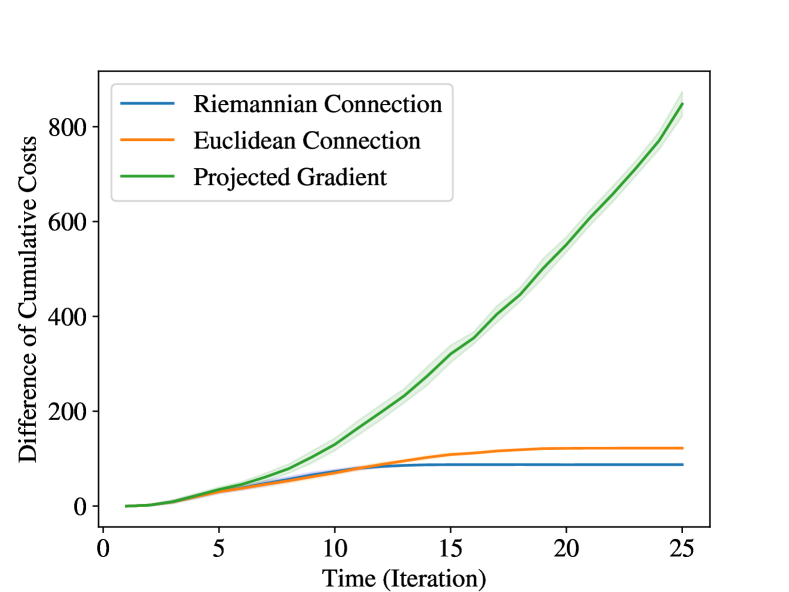
Simulation Setup: We consider a dynamical system with state size $n=6$ and input size $m=3$. The system matrices $(\mathbf{A},\mathbf{B})$ is sampled from a normal distribution with zero mean and unit variance, and $\mathbf{A}$ is scaled to ensure that the system is open-loop stable. For the constraint we consider the sparsity requirement where half of the elements of the controller are forced to be zero (randomly selected). The function sequence consists of 100 $(\mathbf{Q}_{t},\mathbf{R}_{t})$ pairs and to ensure the corresponding (local) minimizer sequence is slowly-varying, $\mathbf{Q}_{t}$ ($\mathbf{R}_{t}$) is constructed by creating a noise matrix $\mathbf{N}$ where each element follows the uniform distribution between 00 and $1$, and then adding $\mathbf{I}$ to $\mathbf{N}\mathbf{N}^{\top}$ scaled with a factor inversely proportional to the total time horizon. As there are no closed form solutions for the constrained setup, we compute the minimizers numerically with gradient norms smaller than a given threshold. In this experiment, we compare three different online approaches: 1) OONM; 2) the second order method where the Hessian operator is defined based on Euclidean connection; 3) the project gradient method (PG) studied in . For the optimistic part, we let $h^{p}_{t+1}=h_{t}$. The step size of all three applied approaches is chosen to satisfy the stability certificate s๐Šsubscript๐‘ ๐Šs_{\mathbf{K}} (see [1] for more details). Given the pre-defined $(\mathbf{A},\mathbf{B})$, $\{(\mathbf{Q}_{t},\mathbf{R}_{t})\}$ and the sparsity requirement, we repeat the learning process for 50 Monte-Carlo simulations and compute the expected cumulative costs.
Performance: From Fig. 1, we can see that the cumulative cost difference of PG is increasing over time as the update direction solely based on first order information can not capture the function landscape precisely. As for the superior performance of OONM with respective to the one with Euclidean connection, it is expected as the Riemannian connection is compatible with the metric arising from the inherent geometry.

VI Conclusion

In this work, we studied the linearly constrained online LQG problem, and we proposed an online second order method based on the problem-related Riemannian metric and the prediction on future cost functions. For the performance guarantee, we present a dynamic regret bound in terms of the minimizersโ€™ path length and the prediction mismatch. We also provide simulation result showing the superiority of the proposed method compared to the Newton method with Euclidean connection and the projected gradient descent. For future directions, it is interesting to see if the current setup can be extended to the decentralized case to accommodate more practical conditions. Another direction to explore is to consider the setup where the dynamics is unknown and see how the Riemannian metric built on system estimates would affect the performance.

VII Appendix

Proof:

For brevity, we first define the following notations:

๐”ผโ€‹[๐ฑtโŠคโ€‹๐ฑt]=๐—t,๐”ผ[๐ฑtsโŠค๐ฑts]=๐—ts,๐”ผโ€‹[๐ฑtโˆ—โŠคโ€‹๐ฑtโˆ—]=๐—tโˆ—,๐”ผ[๐ฑtโˆ—sโŠค๐ฑtโˆ—s]=๐—tโˆ—s,formulae-sequence๐”ผdelimited-[]superscriptsubscript๐ฑ๐‘กtopsubscript๐ฑ๐‘กsubscript๐—๐‘กformulae-sequence๐”ผdelimited-[]superscriptsubscript๐ฑ๐‘กlimit-from๐‘ topsuperscriptsubscript๐ฑ๐‘ก๐‘ subscriptsuperscript๐—๐‘ ๐‘กformulae-sequence๐”ผdelimited-[]superscriptsubscript๐ฑ๐‘กabsenttopsuperscriptsubscript๐ฑ๐‘กsubscriptsuperscript๐—๐‘ก๐”ผdelimited-[]superscriptsubscript๐ฑ๐‘กabsentlimit-from๐‘ topsuperscriptsubscript๐ฑ๐‘กabsent๐‘ subscriptsuperscript๐—absent๐‘ ๐‘ก\begin{split}\mathbb{E}\left[\mathbf{x}_{t}^{\top}\mathbf{x}_{t}\right]=\mathbf{X}_{t}&,\mathbb{E}\left[\mathbf{x}_{t}^{s\top}\mathbf{x}_{t}^{s}\right]=\mathbf{X}^{s}_{t},\\ \mathbb{E}\left[\mathbf{x}_{t}^{*\top}\mathbf{x}_{t}^{*}\right]=\mathbf{X}^{*}_{t}&,\mathbb{E}\left[\mathbf{x}_{t}^{*s\top}\mathbf{x}_{t}^{*s}\right]=\mathbf{X}^{*s}_{t},\end{split}

where $\mathbf{x}_{t+1}=(\mathbf{A}+\mathbf{B}\mathbf{K}_{t})\mathbf{x}_{t}+\mathbf{w}_{t}$, $\mathbf{x}^{*}_{t+1}=(\mathbf{A}+\mathbf{B}\mathbf{K}^{*}_{t})\mathbf{x}^{*}_{t}+\mathbf{w}_{t}$, ๐ฑtssubscriptsuperscript๐ฑ๐‘ ๐‘ก\mathbf{x}^{s}_{t}(๐ฑtโˆ—ssubscriptsuperscript๐ฑabsent๐‘ ๐‘ก\mathbf{x}^{*s}_{t}) follows the steady state distribution of using $\mathbf{K}_{t}$($\mathbf{K}^{*}_{t}$) as a fix controller from the beginning.

The regret is then decomposed into three difference terms and we will provide the upper bound for each one:

๐”ผโ€‹[โˆ‘t=1T(๐ฑtโŠคโ€‹๐tโ€‹๐ฑt+๐ฎtโŠคโ€‹๐‘tโ€‹๐ฎt)โˆ’(๐ฑtโˆ—โŠคโ€‹๐tโ€‹๐ฑtโˆ—+๐ฎtโˆ—โŠคโ€‹๐‘tโ€‹๐ฎtโˆ—)]=โˆ‘t=1T[Trโ€‹((๐t+๐ŠtโŠคโ€‹๐‘tโ€‹๐Št)โ€‹๐—t)โˆ’Trโ€‹((๐t+๐ŠtโŠคโ€‹๐‘tโ€‹๐Št)โ€‹๐—ts)]+โˆ‘t=1T[Trโ€‹((๐t+๐ŠtโŠคโ€‹๐‘tโ€‹๐Št)โ€‹๐—ts)โˆ’Trโ€‹((๐t+๐Štโˆ—โŠคโ€‹๐‘tโ€‹๐Štโˆ—)โ€‹๐—tโˆ—s)]+โˆ‘t=1T[Trโ€‹((๐t+๐Štโˆ—โŠคโ€‹๐‘tโ€‹๐Štโˆ—)โ€‹๐—tโˆ—s)โˆ’Trโ€‹((๐t+๐Štโˆ—โŠคโ€‹๐‘tโ€‹๐Štโˆ—)โ€‹๐—tโˆ—)],๐”ผdelimited-[]superscriptsubscript๐‘ก1๐‘‡superscriptsubscript๐ฑ๐‘กtopsubscript๐๐‘กsubscript๐ฑ๐‘กsuperscriptsubscript๐ฎ๐‘กtopsubscript๐‘๐‘กsubscript๐ฎ๐‘กsuperscriptsubscript๐ฑ๐‘กabsenttopsubscript๐๐‘กsubscriptsuperscript๐ฑ๐‘กsuperscriptsubscript๐ฎ๐‘กabsenttopsubscript๐‘๐‘กsubscriptsuperscript๐ฎ๐‘กsuperscriptsubscript๐‘ก1๐‘‡delimited-[]Trsubscript๐๐‘กsubscriptsuperscript๐Štop๐‘กsubscript๐‘๐‘กsubscript๐Š๐‘กsubscript๐—๐‘กTrsubscript๐๐‘กsubscriptsuperscript๐Štop๐‘กsubscript๐‘๐‘กsubscript๐Š๐‘กsubscriptsuperscript๐—๐‘ ๐‘กsuperscriptsubscript๐‘ก1๐‘‡delimited-[]Trsubscript๐๐‘กsubscriptsuperscript๐Štop๐‘กsubscript๐‘๐‘กsubscript๐Š๐‘กsubscriptsuperscript๐—๐‘ ๐‘กTrsubscript๐๐‘กsubscriptsuperscript๐Šabsenttop๐‘กsubscript๐‘๐‘กsubscriptsuperscript๐Š๐‘กsubscriptsuperscript๐—absent๐‘ ๐‘กsuperscriptsubscript๐‘ก1๐‘‡delimited-[]Trsubscript๐๐‘กsubscriptsuperscript๐Šabsenttop๐‘กsubscript๐‘๐‘กsubscriptsuperscript๐Š๐‘กsubscriptsuperscript๐—absent๐‘ ๐‘กTrsubscript๐๐‘กsubscriptsuperscript๐Šabsenttop๐‘กsubscript๐‘๐‘กsubscriptsuperscript๐Š๐‘กsubscriptsuperscript๐—๐‘ก\begin{split}&\mathbb{E}\left[\sum_{t=1}^{T}(\mathbf{x}_{t}^{\top}\mathbf{Q}_{t}\mathbf{x}_{t}+\mathbf{u}_{t}^{\top}\mathbf{R}_{t}\mathbf{u}_{t})-({\mathbf{x}}_{t}^{*\top}\mathbf{Q}_{t}\mathbf{x}^{*}_{t}+\mathbf{u}_{t}^{*\top}\mathbf{R}_{t}\mathbf{u}^{*}_{t})\right]\\ =&\sum_{t=1}^{T}\left[\text{Tr}\big{(}(\mathbf{Q}_{t}+\mathbf{K}^{\top}_{t}\mathbf{R}_{t}\mathbf{K}_{t})\mathbf{X}_{t}\big{)}-\text{Tr}\big{(}(\mathbf{Q}_{t}+\mathbf{K}^{\top}_{t}\mathbf{R}_{t}\mathbf{K}_{t})\mathbf{X}^{s}_{t}\big{)}\right]\\ +&\sum_{t=1}^{T}\left[\text{Tr}\big{(}(\mathbf{Q}_{t}+\mathbf{K}^{\top}_{t}\mathbf{R}_{t}\mathbf{K}_{t})\mathbf{X}^{s}_{t}\big{)}-\text{Tr}\big{(}(\mathbf{Q}_{t}+\mathbf{K}^{*\top}_{t}\mathbf{R}_{t}\mathbf{K}^{*}_{t})\mathbf{X}^{*s}_{t}\big{)}\right]\\ +&\sum_{t=1}^{T}\left[\text{Tr}\big{(}(\mathbf{Q}_{t}+\mathbf{K}^{*\top}_{t}\mathbf{R}_{t}\mathbf{K}^{*}_{t})\mathbf{X}^{*s}_{t}\big{)}-\text{Tr}\big{(}(\mathbf{Q}_{t}+\mathbf{K}^{*\top}_{t}\mathbf{R}_{t}\mathbf{K}^{*}_{t})\mathbf{X}^{*}_{t}\big{)}\right],\end{split}

which we denote as term I, term II and term III, respectively. Term II: Based on Lemma 5, we have

$$\begin{split}&\text{dist}(\tilde{\mathbf{K}}_{t+1},\mathbf{K}^{*}_{t+1})^{2}\\ \leq&\alpha^{2}\text{dist}(\tilde{\mathbf{K}}_{t},\mathbf{K}^{*}_{t+1})^{2}\\ \leq&\alpha^{2}\left[2\text{dist}(\tilde{\mathbf{K}}_{t},\mathbf{K}^{*}_{t})^{2}+2\text{dist}(\mathbf{K}^{*}_{t},\mathbf{K}^{*}_{t+1})^{2}\right],\end{split}$$ (4)

where $\text{dist}(\cdot,\cdot)$ denotes the Riemannian distance based on the metric $g$. Then by summing Equation (4) over $t$, we can get

$$\begin{split}&\sum_{t=2}^{T}\text{dist}(\tilde{\mathbf{K}}_{t},\mathbf{K}^{*}_{t})^{2}\\ \leq&2\alpha^{2}\sum_{t=1}^{T-1}\text{dist}(\tilde{\mathbf{K}}_{t},\mathbf{K}^{*}_{t})^{2}+2\alpha^{2}\sum_{t=2}^{T}\text{dist}(\mathbf{K}^{*}_{t},\mathbf{K}^{*}_{t-1})^{2}.\end{split}$$ (5)

Adding and subtracting $2\alpha^{2}\text{dist}(\tilde{\mathbf{K}}_{T},\mathbf{K}^{*}_{T})^{2}$ to the right hand side, we get

$$\begin{split}&\sum_{t=1}^{T}\text{dist}(\tilde{\mathbf{K}}_{t},\mathbf{K}^{*}_{t})^{2}\\ \leq&\text{dist}(\tilde{\mathbf{K}}_{1},\mathbf{K}^{*}_{1})^{2}-2\alpha^{2}\text{dist}(\tilde{\mathbf{K}}_{T},\mathbf{K}^{*}_{T})^{2}\\ +&2\alpha^{2}\sum_{t=1}^{T}\text{dist}(\tilde{\mathbf{K}}_{t},\mathbf{K}^{*}_{t})^{2}+2\alpha^{2}\sum_{t=2}^{T}\text{dist}(\mathbf{K}^{*}_{t},\mathbf{K}^{*}_{t-1})^{2}.\end{split}$$ (6)

Choosing $\alpha$ such that $2\alpha^{2}<1$, Eq (6) can be regrouped as follows

$$\begin{split}\sum_{t=1}^{T}\text{dist}(\tilde{\mathbf{K}}_{t},\mathbf{K}^{*}_{t})^{2}\leq&\frac{\text{dist}(\tilde{\mathbf{K}}_{1},\mathbf{K}^{*}_{1})^{2}-2\alpha^{2}\text{dist}(\tilde{\mathbf{K}}_{T},\mathbf{K}^{*}_{T})^{2}}{1-2\alpha^{2}}\\ +&\frac{2\alpha^{2}}{1-2\alpha^{2}}\sum_{t=2}^{T}\text{dist}(\mathbf{K}^{*}_{t},\mathbf{K}^{*}_{t-1})^{2}.\end{split}$$ (7)

Based on the function reformulation of LQG problems, we can see Trโ€‹((๐t+๐ŠtโŠคโ€‹๐‘tโ€‹๐Št)โ€‹๐—ts)=htโ€‹(๐Št)Trsubscript๐๐‘กsubscriptsuperscript๐Štop๐‘กsubscript๐‘๐‘กsubscript๐Š๐‘กsubscriptsuperscript๐—๐‘ ๐‘กsubscriptโ„Ž๐‘กsubscript๐Š๐‘ก\text{Tr}\big{(}(\mathbf{Q}_{t}+\mathbf{K}^{\top}_{t}\mathbf{R}_{t}\mathbf{K}_{t})\mathbf{X}^{s}_{t}\big{)}=h_{t}(\mathbf{K}_{t}) and Trโ€‹((๐t+๐Štโˆ—โŠคโ€‹๐‘tโ€‹๐Štโˆ—)โ€‹๐—tโˆ—s)=htโ€‹(๐Štโˆ—)Trsubscript๐๐‘กsubscriptsuperscript๐Šabsenttop๐‘กsubscript๐‘๐‘กsubscriptsuperscript๐Š๐‘กsubscriptsuperscript๐—absent๐‘ ๐‘กsubscriptโ„Ž๐‘กsubscriptsuperscript๐Š๐‘ก\text{Tr}\big{(}(\mathbf{Q}_{t}+\mathbf{K}^{*\top}_{t}\mathbf{R}_{t}\mathbf{K}^{*}_{t})\mathbf{X}^{*s}_{t}\big{)}=h_{t}(\mathbf{K}^{*}_{t}). Then term II can be expressed as $\sum_{t=1}^{T}h_{t}({\mathbf{K}}_{t})-h_{t}(\mathbf{K}^{*}_{t})$. As the proof of Lemma 5, select a tangent vector $F_{t}\in T_{{\mathbf{K}}_{t}}\tilde{\mathcal{S}}$ such that the curve $\xi(\eta):=\exp_{{\mathbf{K}}_{t}}[\eta F_{t}]$ is the geodesic between ${\mathbf{K}}_{t}$($\xi(0)$) and $\mathbf{K}^{*}_{t}$($\xi(1)$) and $\xi^{\prime}(0)=F_{t}$. Based on this parameterization, we have

$$\begin{split}&h_{t}({\mathbf{K}}_{t})-h_{t}(\mathbf{K}^{*}_{t})\\ =&\int_{\eta=0}^{1}\langle\text{grad }{h_{t}}_{\xi(\eta)},\xi^{\prime}(\eta)\rangle d\eta\\ =&\int_{\eta=0}^{1}\langle\text{grad }{h_{t}}_{\xi(\eta)}-\mathcal{P}^{\xi}_{1,\eta}\text{grad }{h_{t}}_{\xi(1)},\xi^{\prime}(\eta)\rangle d\eta\\ \leq&\int_{\eta=0}^{1}(1-\eta)L_{g}\left\lVert F_{t}\right\rVert_{g_{\xi(0)}}\left\lVert\xi^{\prime}(\eta)\right\rVert_{g_{\xi(\eta)}}d\eta\\ =&\int_{\eta=0}^{1}(1-\eta)L_{g}\left\lVert F_{t}\right\rVert^{2}_{g_{\xi(0)}}d\eta\\ =&\frac{L_{g}}{2}\left\lVert F_{t}\right\rVert^{2}_{g_{{\mathbf{K}}_{t}}},\end{split}$$ (8)

where the inequality is due to the smoothness of $\text{grad }{h_{t}}_{\xi(\eta)}$ in $\eta$ and the fact that the size of the derivative of geodesic stays constant. Note that $\left\lVert F_{t}\right\rVert_{g_{{\mathbf{K}}_{t}}}=\text{dist}({\mathbf{K}}_{t},\mathbf{K}^{*}_{t})$. By summing Eq (8) over $t$, we show

$$\begin{split}&\sum_{t=1}^{T}h_{t}({\mathbf{K}}_{t})-h_{t}(\mathbf{K}^{*}_{t})\\ \leq&\frac{L_{g}}{2}\sum_{t=1}^{T}\text{dist}({\mathbf{K}}_{t},\mathbf{K}^{*}_{t})^{2}\\ \leq&\frac{L_{g}}{2}\sum_{t=1}^{T}\left[2\text{dist}({\mathbf{K}}_{t},\tilde{\mathbf{K}}_{t})^{2}+2\text{dist}(\tilde{\mathbf{K}}_{t},\mathbf{K}^{*}_{t})^{2}\right]\\ \leq&L_{g}\sum_{t=1}^{t}\text{dist}({\mathbf{K}}_{t},\tilde{\mathbf{K}}_{t})^{2}+\frac{2L_{g}\alpha^{2}}{1-2\alpha^{2}}\sum_{t=2}^{T}\text{dist}(\mathbf{K}^{*}_{t},\mathbf{K}^{*}_{t-1})^{2}\\ +&L_{g}\left[\frac{\text{dist}(\tilde{\mathbf{K}}_{1},\mathbf{K}^{*}_{1})^{2}-2\alpha^{2}\text{dist}(\tilde{\mathbf{K}}_{T},\mathbf{K}^{*}_{T})^{2}}{1-2\alpha^{2}}\right]\\ =&L_{g}\left[\frac{\text{dist}(\tilde{\mathbf{K}}_{1},\mathbf{K}^{*}_{1})^{2}-2\alpha^{2}\text{dist}(\tilde{\mathbf{K}}_{T},\mathbf{K}^{*}_{T})^{2}}{1-2\alpha^{2}}\right]\\ +&\frac{2L_{g}\alpha^{2}}{1-2\alpha^{2}}\sum_{t=2}^{T}\text{dist}(\mathbf{K}^{*}_{t},\mathbf{K}^{*}_{t-1})^{2}\\ +&L_{g}\eta_{0}\left\lVert G_{0}\right\rVert^{2}_{g_{\tilde{\mathbf{K}}_{0}}}+L_{g}\sum_{t=1}^{T-1}\eta_{t}\left\lVert G^{p}_{t}-G_{t}\right\rVert^{2}_{g_{\tilde{\mathbf{K}}_{t}}},\end{split}$$ (9)

where the third inequality is based on Equation (7) and the last equality can be shown based on the update rule.
Term I and Term III: Suppose that the controller sequence $\{\mathbf{K}_{t}\}$ satisfies the condition that $\mathbf{K}_{t}$ lies in $\mathcal{U}_{t}$ for all $t$ and let $\kappa=\sqrt{\nu}/\sigma$. Assume that โˆฅ๐—t+1sโˆ’๐—tsโˆฅโ‰คฮถdelimited-โˆฅโˆฅsubscriptsuperscript๐—๐‘ ๐‘ก1subscriptsuperscript๐—๐‘ ๐‘ก๐œ\left\lVert\mathbf{X}^{s}_{t+1}-\mathbf{X}^{s}_{t}\right\rVert\leq\zeta for all $t$ for some $\zeta\leq\sigma^{2}/\kappa^{2}$. Then by following the derivations of Lemmas 4.3 and 4.4 in [3], it can be shown that the controller sequence $\{\mathbf{K}_{t}\}$ is $(\kappa,\frac{1}{2\kappa^{2}})$ sequentially strongly stable. Then based on the derivation of Lemma 3.5 in [3], it can be shown that

โˆฅ๐—tโˆ’๐—tsโˆฅโ‰คฮบ2โ€‹expโˆ’t2โ€‹ฮบ2โกโˆฅ๐—1โˆ’๐—1sโˆฅ+4โ€‹ฮบ4โ€‹ฮถ.delimited-โˆฅโˆฅsubscript๐—๐‘กsubscriptsuperscript๐—๐‘ ๐‘กsuperscript๐œ…2superscript๐‘ก2superscript๐œ…2subscript๐—1subscriptsuperscript๐—๐‘ 14superscript๐œ…4๐œ\left\lVert\mathbf{X}_{t}-\mathbf{X}^{s}_{t}\right\rVert\leq\kappa^{2}\exp^{\frac{-t}{2\kappa^{2}}}\left\lVert\mathbf{X}_{1}-\mathbf{X}^{s}_{1}\right\rVert+4\kappa^{4}\zeta. (10)

Since through the all analysis, we are considering the case where for all $t$, $\mathbf{K}_{t}$ is within a bounded region w.r.t. $\mathbf{K}^{*}_{t}$ in terms of the distance function defined on the riemannian metric, we assume there exists a positive constant Lssubscript๐ฟ๐‘ L_{s} such that โˆฅ๐—t+1sโˆ’๐—tsโˆฅโ‰คLsโ€‹distโ€‹(๐Št+1,๐Št)delimited-โˆฅโˆฅsubscriptsuperscript๐—๐‘ ๐‘ก1subscriptsuperscript๐—๐‘ ๐‘กsubscript๐ฟ๐‘ distsubscript๐Š๐‘ก1subscript๐Š๐‘ก\left\lVert\mathbf{X}^{s}_{t+1}-\mathbf{X}^{s}_{t}\right\rVert\leq L_{s}\text{dist}(\mathbf{K}_{t+1},\mathbf{K}_{t}). Therefore, to ensure Eq (10), it is sufficient to define $\zeta_{1}:=\max_{t}\left[\text{dist}(\mathbf{K}_{t+1},\mathbf{K}_{t})\right]$ and make Lsโ€‹ฮถ1subscript๐ฟ๐‘ subscript๐œ1L_{s}\zeta_{1} upper-bounded by $\sigma^{2}/\kappa^{2}$. Based on Equation (10), we have

โˆ‘t=1T[Trโ€‹((๐t+๐ŠtโŠคโ€‹๐‘tโ€‹๐Št)โ€‹๐—t)โˆ’Trโ€‹((๐t+๐ŠtโŠคโ€‹๐‘tโ€‹๐Št)โ€‹๐—ts)]โ‰คโˆ‘t=1TTrโ€‹(๐t+๐ŠtโŠคโ€‹๐‘tโ€‹๐Št)โ€‹โˆฅ๐—tโˆ’๐—tsโˆฅโ‰คCโ€‹(1+ฮบ2)โ€‹โˆ‘t=1T[ฮบ2โ€‹expโˆ’t2โ€‹ฮบ2โกโˆฅ๐—1โˆ’๐—1sโˆฅ+4โ€‹ฮบ4โ€‹Lsโ€‹ฮถ1],superscriptsubscript๐‘ก1๐‘‡delimited-[]Trsubscript๐๐‘กsubscriptsuperscript๐Štop๐‘กsubscript๐‘๐‘กsubscript๐Š๐‘กsubscript๐—๐‘กTrsubscript๐๐‘กsubscriptsuperscript๐Štop๐‘กsubscript๐‘๐‘กsubscript๐Š๐‘กsubscriptsuperscript๐—๐‘ ๐‘กsuperscriptsubscript๐‘ก1๐‘‡Trsubscript๐๐‘กsubscriptsuperscript๐Štop๐‘กsubscript๐‘๐‘กsubscript๐Š๐‘กdelimited-โˆฅโˆฅsubscript๐—๐‘กsubscriptsuperscript๐—๐‘ ๐‘ก๐ถ1superscript๐œ…2superscriptsubscript๐‘ก1๐‘‡delimited-[]superscript๐œ…2superscript๐‘ก2superscript๐œ…2subscript๐—1subscriptsuperscript๐—๐‘ 14superscript๐œ…4subscript๐ฟ๐‘ subscript๐œ1\begin{split}&\sum_{t=1}^{T}\left[\text{Tr}\big{(}(\mathbf{Q}_{t}+\mathbf{K}^{\top}_{t}\mathbf{R}_{t}\mathbf{K}_{t})\mathbf{X}_{t}\big{)}-\text{Tr}\big{(}(\mathbf{Q}_{t}+\mathbf{K}^{\top}_{t}\mathbf{R}_{t}\mathbf{K}_{t})\mathbf{X}^{s}_{t}\big{)}\right]\\ \leq&\sum_{t=1}^{T}\text{Tr}(\mathbf{Q}_{t}+\mathbf{K}^{\top}_{t}\mathbf{R}_{t}\mathbf{K}_{t})\left\lVert\mathbf{X}_{t}-\mathbf{X}^{s}_{t}\right\rVert\\ \leq&C(1+\kappa^{2})\sum_{t=1}^{T}\left[\kappa^{2}\exp^{\frac{-t}{2\kappa^{2}}}\left\lVert\mathbf{X}_{1}-\mathbf{X}^{s}_{1}\right\rVert+4\kappa^{4}L_{s}\zeta_{1}\right],\end{split} (11)

where the last inequality is based on $\text{Tr}(\mathbf{Q}_{t}),\text{Tr}(\mathbf{R}_{t})\leq C$ and $\mathbf{K}_{t}$ is $(\kappa,\gamma)$-strongly stable.
As Equation (10), if โˆ€t,โˆฅ๐—t+1โˆ—sโˆ’๐—tโˆ—sโˆฅโ‰คฮถfor-all๐‘กdelimited-โˆฅโˆฅsubscriptsuperscript๐—absent๐‘ ๐‘ก1subscriptsuperscript๐—absent๐‘ ๐‘ก๐œ\forall t,\;\left\lVert\mathbf{X}^{*s}_{t+1}-\mathbf{X}^{*s}_{t}\right\rVert\leq\zeta for some $\zeta\leq\sigma^{2}/\kappa^{2}$, then we also have

โˆฅ๐—tโˆ—โˆ’๐—tโˆ—sโˆฅโ‰คฮบ2โ€‹expโˆ’t2โ€‹ฮบ2โกโˆฅ๐—1โˆ—โˆ’๐—1โˆ—sโˆฅ+4โ€‹ฮบ4โ€‹ฮถ.delimited-โˆฅโˆฅsubscriptsuperscript๐—๐‘กsubscriptsuperscript๐—absent๐‘ ๐‘กsuperscript๐œ…2superscript๐‘ก2superscript๐œ…2subscriptsuperscript๐—1subscriptsuperscript๐—absent๐‘ 14superscript๐œ…4๐œ\left\lVert\mathbf{X}^{*}_{t}-\mathbf{X}^{*s}_{t}\right\rVert\leq\kappa^{2}\exp^{\frac{-t}{2\kappa^{2}}}\left\lVert\mathbf{X}^{*}_{1}-\mathbf{X}^{*s}_{1}\right\rVert+4\kappa^{4}\zeta. (12)

By the smoothness of the steady-state covariance matrix, there also exists a positive constant Lssubscript๐ฟ๐‘ L_{s} such that โˆฅ๐—t+1โˆ—sโˆ’๐—tโˆ—sโˆฅโ‰คLsโ€‹distโ€‹(๐Št+1โˆ—,๐Štโˆ—)delimited-โˆฅโˆฅsubscriptsuperscript๐—absent๐‘ ๐‘ก1subscriptsuperscript๐—absent๐‘ ๐‘กsubscript๐ฟ๐‘ distsubscriptsuperscript๐Š๐‘ก1subscriptsuperscript๐Š๐‘ก\left\lVert\mathbf{X}^{*s}_{t+1}-\mathbf{X}^{*s}_{t}\right\rVert\leq L_{s}\text{dist}(\mathbf{K}^{*}_{t+1},\mathbf{K}^{*}_{t}). Therefore, to ensure Equation (12), we can define $\zeta_{2}:=\max_{t}\left[\text{dist}(\mathbf{K}^{*}_{t+1},\mathbf{K}^{*}_{t})\right]$ and let Lsโ€‹ฮถ2subscript๐ฟ๐‘ subscript๐œ2L_{s}\zeta_{2} upper-bounded by $\sigma^{2}/\kappa^{2}$, and then we also have

โˆ‘t=1T[Trโ€‹((๐t+๐Štโˆ—โŠคโ€‹๐‘tโ€‹๐Štโˆ—)โ€‹๐—tโˆ—)โˆ’Trโ€‹((๐t+๐Štโˆ—โŠคโ€‹๐‘tโ€‹๐Štโˆ—)โ€‹๐—tโˆ—s)]โ‰คโˆ‘t=1TTrโ€‹(๐t+๐Štโˆ—โŠคโ€‹๐‘tโ€‹๐Štโˆ—)โ€‹โˆฅ๐—tโˆ—โˆ’๐—tโˆ—sโˆฅโ‰คCโ€‹(1+ฮบ2)โ€‹โˆ‘t=1T[ฮบ2โ€‹expโˆ’t2โ€‹ฮบ2โกโˆฅ๐—1โˆ—โˆ’๐—1โˆ—sโˆฅ+4โ€‹ฮบ4โ€‹Lsโ€‹ฮถ2],superscriptsubscript๐‘ก1๐‘‡delimited-[]Trsubscript๐๐‘กsubscriptsuperscript๐Šabsenttop๐‘กsubscript๐‘๐‘กsubscriptsuperscript๐Š๐‘กsubscriptsuperscript๐—๐‘กTrsubscript๐๐‘กsubscriptsuperscript๐Šabsenttop๐‘กsubscript๐‘๐‘กsubscriptsuperscript๐Š๐‘กsubscriptsuperscript๐—absent๐‘ ๐‘กsuperscriptsubscript๐‘ก1๐‘‡Trsubscript๐๐‘กsubscriptsuperscript๐Šabsenttop๐‘กsubscript๐‘๐‘กsubscriptsuperscript๐Š๐‘กdelimited-โˆฅโˆฅsubscriptsuperscript๐—๐‘กsubscriptsuperscript๐—absent๐‘ ๐‘ก๐ถ1superscript๐œ…2superscriptsubscript๐‘ก1๐‘‡delimited-[]superscript๐œ…2superscript๐‘ก2superscript๐œ…2subscriptsuperscript๐—1subscriptsuperscript๐—absent๐‘ 14superscript๐œ…4subscript๐ฟ๐‘ subscript๐œ2\begin{split}&\sum_{t=1}^{T}\left[\text{Tr}\big{(}(\mathbf{Q}_{t}+\mathbf{K}^{*\top}_{t}\mathbf{R}_{t}\mathbf{K}^{*}_{t})\mathbf{X}^{*}_{t}\big{)}-\text{Tr}\big{(}(\mathbf{Q}_{t}+\mathbf{K}^{*\top}_{t}\mathbf{R}_{t}\mathbf{K}^{*}_{t})\mathbf{X}^{*s}_{t}\big{)}\right]\\ \leq&\sum_{t=1}^{T}\text{Tr}(\mathbf{Q}_{t}+\mathbf{K}^{*\top}_{t}\mathbf{R}_{t}\mathbf{K}^{*}_{t})\left\lVert\mathbf{X}^{*}_{t}-\mathbf{X}^{*s}_{t}\right\rVert\\ \leq&C(1+\kappa^{2})\sum_{t=1}^{T}\left[\kappa^{2}\exp^{\frac{-t}{2\kappa^{2}}}\left\lVert\mathbf{X}^{*}_{1}-\mathbf{X}^{*s}_{1}\right\rVert+4\kappa^{4}L_{s}\zeta_{2}\right],\end{split} (13)

Based on Equations (9), (11) and (13), we can show the regret bound is

$$O\left(T(\zeta_{1}+\zeta_{2})+\sum_{t=2}^{T}\text{dist}(\mathbf{K}^{*}_{t},\mathbf{K}^{*}_{t-1})^{2}+\sum_{t=1}^{T-1}\left\lVert G^{p}_{t}-G_{t}\right\rVert^{2}_{g_{\tilde{\mathbf{K}}_{t}}}\right).$$

โˆŽ

References

  • [1] S.ย Talebi and M.ย Mesbahi, โ€œPolicy optimization over submanifolds for linearly constrained feedback synthesis,โ€ IEEE Transactions on Automatic Control, 2023.
  • [2] B.ย D.ย O. Anderson, J.ย B. Moore, and B.ย P. Molinari, โ€œLinear optimal control,โ€ IEEE Transactions on Systems, Man, and Cybernetics, vol. SMC-2, no.ย 4, pp. 559โ€“559, 1972.
  • [3] A.ย Cohen, A.ย Hasidim, T.ย Koren, N.ย Lazic, Y.ย Mansour, and K.ย Talwar, โ€œOnline linear quadratic control,โ€ in International Conference on Machine Learning, 2018, pp. 1029โ€“1038.
  • [4] N.ย Agarwal, B.ย Bullins, E.ย Hazan, S.ย M. Kakade, and K.ย Singh, โ€œOnline control with adversarial disturbances,โ€ in 36th International Conference on Machine Learning, ICML 2019.ย ย ย International Machine Learning Society (IMLS), 2019, pp. 154โ€“165.
  • [5] N.ย Agarwal, E.ย Hazan, and K.ย Singh, โ€œLogarithmic regret for online control,โ€ in Advances in Neural Information Processing Systems, 2019, pp. 10โ€‰175โ€“10โ€‰184.
  • [6] M.ย Simchowitz, K.ย Singh, and E.ย Hazan, โ€œImproper learning for non-stochastic control,โ€ arXiv preprint arXiv:2001.09254, 2020.
  • [7] T.-J. Chang and S.ย Shahrampour, โ€œDistributed online linear quadratic control for linear time-invariant systems,โ€ in American Control Conference (ACC), 2021, pp. 923โ€“928.
  • [8] M.ย Fazel, R.ย Ge, S.ย Kakade, and M.ย Mesbahi, โ€œGlobal convergence of policy gradient methods for the linear quadratic regulator,โ€ in International Conference on Machine Learning, 2018, pp. 1467โ€“1476.
  • [9] J.ย Bu, A.ย Mesbahi, M.ย Fazel, and M.ย Mesbahi, โ€œLqr through the lens of first order methods: Discrete-time case,โ€ arXiv preprint arXiv:1907.08921, 2019.
  • [10] J.ย Bu, A.ย Mesbahi, and M.ย Mesbahi, โ€œPolicy gradient-based algorithms for continuous-time linear quadratic control,โ€ arXiv preprint arXiv:2006.09178, 2020.
  • [11] H.ย Mohammadi, A.ย Zare, M.ย Soltanolkotabi, and M.ย R. Jovanoviฤ‡, โ€œConvergence and sample complexity of gradient methods for the model-free linearโ€“quadratic regulator problem,โ€ IEEE Transactions on Automatic Control, vol.ย 67, no.ย 5, pp. 2435โ€“2450, 2021.
  • [12] M.ย Zinkevich, โ€œOnline convex programming and generalized infinitesimal gradient ascent,โ€ in Proceedings of the 20th international conference on machine learning (icml-03), 2003, pp. 928โ€“936.
  • [13] E.ย Hazan, A.ย Agarwal, and S.ย Kale, โ€œLogarithmic regret algorithms for online convex optimization,โ€ Machine Learning, vol.ย 69, no. 2-3, pp. 169โ€“192, 2007.
  • [14] L.ย Zhang, S.ย Lu, and Z.-H. Zhou, โ€œAdaptive online learning in dynamic environments,โ€ Advances in neural information processing systems, vol.ย 31, 2018.
  • [15] A.ย Mokhtari, S.ย Shahrampour, A.ย Jadbabaie, and A.ย Ribeiro, โ€œOnline optimization in dynamic environments: Improved regret rates for strongly convex problems,โ€ in 2016 IEEE 55th Conference on Decision and Control (CDC).ย ย ย IEEE, 2016, pp. 7195โ€“7201.
  • [16] O.ย Besbes, Y.ย Gur, and A.ย Zeevi, โ€œNon-stationary stochastic optimization,โ€ Operations research, vol.ย 63, no.ย 5, pp. 1227โ€“1244, 2015.
  • [17] C.-K. Chiang, T.ย Yang, C.-J. Lee, M.ย Mahdavi, C.-J. Lu, R.ย Jin, and S.ย Zhu, โ€œOnline optimization with gradual variations,โ€ in Conference on Learning Theory.ย ย ย JMLR Workshop and Conference Proceedings, 2012, pp. 6โ€“1.
  • [18] S.ย Rakhlin and K.ย Sridharan, โ€œOptimization, learning, and games with predictable sequences,โ€ Advances in Neural Information Processing Systems, vol.ย 26, 2013.
  • [19] A.ย Jadbabaie, A.ย Rakhlin, S.ย Shahrampour, and K.ย Sridharan, โ€œOnline optimization: Competing with dynamic comparators,โ€ in Artificial Intelligence and Statistics.ย ย ย PMLR, 2015, pp. 398โ€“406.
  • [20] T.-J. Chang and S.ย Shahrampour, โ€œOn online optimization: Dynamic regret analysis of strongly convex and smooth problems,โ€ in Proceedings of the AAAI Conference on Artificial Intelligence, vol.ย 35, no.ย 8, 2021, pp. 6966โ€“6973.
  • [21] E.ย Hazan, S.ย Kakade, and K.ย Singh, โ€œThe nonstochastic control problem,โ€ in Algorithmic Learning Theory, 2020, pp. 408โ€“421.
  • [22] P.ย Zhao, Y.-X. Wang, and Z.-H. Zhou, โ€œNon-stationary online learning with memory and non-stochastic control,โ€ in International Conference on Artificial Intelligence and Statistics.ย ย ย PMLR, 2022, pp. 2101โ€“2133.
  • [23] D.ย Baby and Y.-X. Wang, โ€œOptimal dynamic regret in lqr control,โ€ Advances in Neural Information Processing Systems, vol.ย 35, pp. 24โ€‰879โ€“24โ€‰892, 2022.
  • [24] Y.ย Luo, V.ย Gupta, and M.ย Kolar, โ€œDynamic regret minimization for control of non-stationary linear dynamical systems,โ€ Proceedings of the ACM on Measurement and Analysis of Computing Systems, vol.ย 6, no.ย 1, pp. 1โ€“72, 2022.
  • [25] Y.ย Li, S.ย Das, and N.ย Li, โ€œOnline optimal control with affine constraints,โ€ in Proceedings of the AAAI Conference on Artificial Intelligence, vol.ย 35, no.ย 10, 2021, pp. 8527โ€“8537.
  • [26] T.ย Li, Y.ย Chen, B.ย Sun, A.ย Wierman, and S.ย H. Low, โ€œInformation aggregation for constrained online control,โ€ Proceedings of the ACM on Measurement and Analysis of Computing Systems, vol.ย 5, no.ย 2, pp. 1โ€“35, 2021.

VIII Supplementary Material

Lemma 5

Suppose the assumptions of Theorem 3 hold, then for $\alpha\in(0,1)$, if $\forall t,\;\text{dist}(\tilde{\mathbf{K}}_{t},\mathbf{K}^{*}_{t+1})\leq\frac{\alpha}{(L_{H}L^{2}/m^{3})}$, then by selecting $\eta_{t}$ such that (1โˆ’ฮฑโ€‹m2โ€‹L)โ‰คฮทtโ‰คminโก{1,s๐Š~t}1๐›ผ๐‘š2๐ฟsubscript๐œ‚๐‘ก1subscript๐‘ subscript~๐Š๐‘ก(1-\frac{\alpha m}{2L})\leq\eta_{t}\leq\min\{1,s_{\tilde{\mathbf{K}}_{t}}\}, the following inequality holds:

$$\text{dist}(\tilde{\mathbf{K}}_{t+1},\mathbf{K}^{*}_{t+1})\leq\alpha\text{dist}(\tilde{\mathbf{K}}_{t},\mathbf{K}^{*}_{t+1}),$$

for $t=0,\ldots,T$.

Proof:

Based on the Hessian assumption and the Cauchy-Schwartz inequality at $\tilde{\mathbf{K}}_{t-1}$, for the Newton direction $G_{t-1}$, we have

$$\begin{split}&m\left\lVert G_{t-1}\right\rVert^{2}_{g_{\tilde{\mathbf{K}}_{t-1}}}\leq\langle\text{Hess }{h_{t}}_{\tilde{\mathbf{K}}_{t-1}}[G_{t-1}],G_{t-1}\rangle\leq\left\lVert\text{grad }{h_{t}}_{\tilde{\mathbf{K}}_{t-1}}\right\rVert_{g_{\tilde{\mathbf{K}}_{t-1}}}\left\lVert G_{t-1}\right\rVert_{g_{\tilde{\mathbf{K}}_{t-1}}}\\ \Rightarrow&\left\lVert G_{t-1}\right\rVert_{g_{\tilde{\mathbf{K}}_{t-1}}}\leq\frac{1}{m}\left\lVert\text{grad }{h_{t}}_{\tilde{\mathbf{K}}_{t-1}}\right\rVert_{g_{\tilde{\mathbf{K}}_{t-1}}}.\end{split}$$ (14)

Define a curve r:[0,s๐Š~tโˆ’1]โ†ฆ๐’ฎ~:๐‘Ÿmaps-to0subscript๐‘ subscript~๐Š๐‘ก1~๐’ฎr:[0,s_{\tilde{\mathbf{K}}_{t-1}}]\mapsto\tilde{\mathcal{S}} such that $r(\eta)=\tilde{\mathbf{K}}_{t-1}+\eta G_{t-1}$ and consider a smooth vector field $E(\eta)$ which is parallel along the curve $r$. Define another a scalar function ฯ•:[0,s๐Š~tโˆ’1]โ†ฆR:italic-ฯ•maps-to0subscript๐‘ subscript~๐Š๐‘ก1R\phi:[0,s_{\tilde{\mathbf{K}}_{t-1}}]\mapsto\mathrm{R} such that $\phi(\eta)=\langle\text{grad }{h_{t}}_{r(\eta)},E(\eta)\rangle$. Based on the smoothness of $\text{grad }{h_{t}}$, we know that $\phi$ is also smooth in $\eta$. Then with the metric compatability, we have

$$\begin{split}&\phi^{\prime}(\eta)\\ =&\langle D_{\eta}\text{grad }{h_{t}}_{r(\eta)},E(\eta)\rangle+\langle\text{grad }{h_{t}}_{r(\eta)},D_{\eta}E(\eta)\rangle\\ =&\langle\text{Hess }{h_{t}}_{r(\eta)}[G_{t-1}],E(\eta)\rangle.\end{split}$$ (15)

where $D_{\eta}$ denotes the covariant derivative operator along the curve $r$ and we note that $G_{t-1}$ is extended to a vector field along $r$ which is constant in the global coordinate frame. Knowing that

$$\phi(\eta)=\phi(0)+\eta\phi^{\prime}(0)+\int_{0}^{\eta}\left(\phi^{\prime}(\tau)-\phi^{\prime}(0)\right)d\tau.$$ (16)

By substituting Eq (15) to Eq (16), we have

$$\begin{split}&\phi(\eta_{t-1})\\ =&\langle\text{grad }{h_{t}}_{\tilde{\mathbf{K}}_{t}},E(\eta_{t-1})\rangle\\ =&(1-\eta_{t-1})\langle\text{grad }{h_{t}}_{\tilde{\mathbf{K}}_{t-1}},E(0)\rangle+\int_{0}^{\eta_{t-1}}\left[\langle\text{Hess }{h_{t}}_{r(\tau)}[G_{t-1}],E(\tau)\rangle-\langle\text{Hess }{h_{t}}_{r(0)}[G_{t-1}],E(0)\rangle\right]d\tau\\ =&(1-\eta_{t-1})\langle\mathcal{P}^{r}_{0,\eta_{t-1}}\text{grad }{h_{t}}_{\tilde{\mathbf{K}}_{t-1}},E(\eta_{t-1})\rangle+\int_{0}^{\eta_{t-1}}\left[\langle\text{Hess }{h_{t}}_{r(\tau)}[G_{t-1}],E(\tau)\rangle-\langle\mathcal{P}^{r}_{0,\tau}\text{Hess }{h_{t}}_{r(0)}[G_{t-1}],E(\tau)\rangle\right]d\tau\\ =&(1-\eta_{t-1})\langle\mathcal{P}^{r}_{0,\eta_{t-1}}\text{grad }{h_{t}}_{\tilde{\mathbf{K}}_{t-1}},E(\eta_{t-1})\rangle+\int_{0}^{\eta_{t-1}}\left[\langle(\text{Hess }{h_{t}}_{r(\tau)}-\mathcal{P}^{r}_{0,\tau}\text{Hess }{h_{t}}_{r(0)})[G_{t-1}],E(\tau)\rangle\right]d\tau,\end{split}$$ (17)

where $\mathcal{P}^{r}_{0,\tau}$ denotes the parallel transport operator from 00 to $\tau$ along the curve $r$ and the second equality is due to the linear isometry property of parallel transport. Noting that $\forall t$, the Hessian operator $\text{Hess }{h_{t}}_{r(\eta)}$ is smoothness in $\eta$, there exists a general constant $L_{H}$ such that

$$\left\lVert(\text{Hess }{h_{t}}_{r(\tau)}-\mathcal{P}^{r}_{0,\tau}\text{Hess }{h_{t}}_{r(0)})[G_{t-1}]\right\rVert_{g_{r(\tau)}}\leq L_{H}\tau\left\lVert G_{t-1}\right\rVert^{2}_{g_{\tilde{\mathbf{K}}_{t-1}}}.$$ (18)

Also since the parallel transport operator conserves the dot product, we have

$$\left\lVert\mathcal{P}^{r}_{0,\eta_{t-1}}\text{grad }{h_{t}}_{\tilde{\mathbf{K}}_{t-1}}\right\rVert_{g_{\tilde{\mathbf{K}}_{t}}}=\left\lVert\text{grad }{h_{t}}_{\tilde{\mathbf{K}}_{t-1}}\right\rVert_{g_{\tilde{\mathbf{K}}_{t-1}}}$$ (19)

Then by choosing the parallel vector field $E(\eta)$ satisfying $E(\eta_{t-1})=\text{grad }{h_{t}}_{\tilde{\mathbf{K}}_{t}}$, based on Eq (18) and Eq (19) we can get

$$\begin{split}\phi(\eta_{t-1})&=\langle\text{grad }{h_{t}}_{\tilde{\mathbf{K}}_{t}},\text{grad }{h_{t}}_{\tilde{\mathbf{K}}_{t}}\rangle\\ &=\left\lVert\text{grad }{h_{t}}_{\tilde{\mathbf{K}}_{t}}\right\rVert^{2}_{g_{\tilde{\mathbf{K}}_{t}}}\\ &\leq(1-\eta_{t-1})\left\lVert\text{grad }{h_{t}}_{\tilde{\mathbf{K}}_{t-1}}\right\rVert_{g_{\tilde{\mathbf{K}}_{t-1}}}\left\lVert\text{grad }{h_{t}}_{\tilde{\mathbf{K}}_{t}}\right\rVert_{g_{\tilde{\mathbf{K}}_{t}}}+\int_{0}^{\eta_{t-1}}\left[L_{H}\tau\left\lVert G_{t-1}\right\rVert^{2}_{g_{\tilde{\mathbf{K}}_{t-1}}}\left\lVert E(\tau)\right\rVert_{g_{r(\tau)}}\right]d\tau\\ &=(1-\eta_{t-1})\left\lVert\text{grad }{h_{t}}_{\tilde{\mathbf{K}}_{t-1}}\right\rVert_{g_{\tilde{\mathbf{K}}_{t-1}}}\left\lVert\text{grad }{h_{t}}_{\tilde{\mathbf{K}}_{t}}\right\rVert_{g_{\tilde{\mathbf{K}}_{t}}}+\int_{0}^{\eta_{t-1}}\left[L_{H}\tau\left\lVert G_{t-1}\right\rVert^{2}_{g_{\tilde{\mathbf{K}}_{t-1}}}\left\lVert\text{grad }{h_{t}}_{\tilde{\mathbf{K}}_{t}}\right\rVert_{g_{\tilde{\mathbf{K}}_{t}}}\right]d\tau\\ &=(1-\eta_{t-1})\left\lVert\text{grad }{h_{t}}_{\tilde{\mathbf{K}}_{t-1}}\right\rVert_{g_{\tilde{\mathbf{K}}_{t-1}}}\left\lVert\text{grad }{h_{t}}_{\tilde{\mathbf{K}}_{t}}\right\rVert_{g_{\tilde{\mathbf{K}}_{t}}}+\frac{\eta_{t-1}^{2}}{2}L_{H}\left\lVert G_{t-1}\right\rVert^{2}_{g_{\tilde{\mathbf{K}}_{t-1}}}\left\lVert\text{grad }{h_{t}}_{\tilde{\mathbf{K}}_{t}}\right\rVert_{g_{\tilde{\mathbf{K}}_{t}}},\end{split}$$ (20)

where the first inequality is based on Cauchy inequality and the last equality is due to the fact that the length of parallel vector field is constant. From Eq (20) we conclude

$$\begin{split}\left\lVert\text{grad }{h_{t}}_{\tilde{\mathbf{K}}_{t}}\right\rVert_{g_{\tilde{\mathbf{K}}_{t}}}&\leq(1-\eta_{t-1})\left\lVert\text{grad }{h_{t}}_{\tilde{\mathbf{K}}_{t-1}}\right\rVert_{g_{\tilde{\mathbf{K}}_{t-1}}}+\frac{\eta_{t-1}^{2}}{2}L_{H}\left\lVert G_{t-1}\right\rVert^{2}_{g_{\tilde{\mathbf{K}}_{t-1}}}\\ &\leq(1-\eta_{t-1})\left\lVert\text{grad }{h_{t}}_{\tilde{\mathbf{K}}_{t-1}}\right\rVert_{g_{\tilde{\mathbf{K}}_{t-1}}}+\frac{\eta^{2}_{t-1}L_{H}}{2m^{2}}\left\lVert\text{grad }{h_{t}}_{\tilde{\mathbf{K}}_{t-1}}\right\rVert^{2}_{g_{\tilde{\mathbf{K}}_{t-1}}}.\end{split}$$ (21)

where the last inequality is based on Eq (14). Next, select a tangent vector $F_{t}\in T_{\tilde{\mathbf{K}}_{t}}\tilde{\mathcal{S}}$ such that the curve $\xi(\eta):=\exp_{\tilde{\mathbf{K}}_{t}}[\eta F_{t}]$ is the geodesic between $\tilde{\mathbf{K}}_{t}$($\xi(0)$) and $\mathbf{K}^{*}_{t}$($\xi(1)$) and $\xi^{\prime}(0)=F_{t}$. Note that the exponential mapping is well-defined if $\tilde{\mathbf{K}}_{t}$ is closed enough to $\mathbf{K}^{*}_{t}$ (the local existence and uniqueness theorem for geodesics). Then for a parallel vector field $E(\eta)$ along $\xi$, define a scalar function $\psi:[0,1]\mapsto\mathrm{R}$ such that $\psi(\eta)=\langle\text{grad }{h_{t}}_{\xi(\eta)},E(\eta)\rangle$. Similiar to Eq (15), we have

$$\psi^{\prime}(\eta)=\langle\text{Hess }{h_{t}}_{\xi(\eta)}[\xi^{\prime}(\eta)],E(\eta)\rangle.$$ (22)

As the velocity of a geodesic curve is parallel, by choosing $E(\eta)=\xi^{\prime}(\eta)$ and based on Eq (22), we get

$$\begin{split}\psi(1)&=\psi(0)+\int_{\tau=0}^{1}\psi^{\prime}(\tau)d\tau\\ &=\langle\text{grad }{h_{t}}_{\tilde{\mathbf{K}}_{t}},F_{t}\rangle+\int_{\tau=0}^{1}\langle\text{Hess }{h_{t}}_{\xi(\tau)}[\xi^{\prime}(\tau)],\xi^{\prime}(\tau)\rangle d\tau.\end{split}$$ (23)

Since $\psi(1)=0$($\tilde{\mathbf{K}}_{t}$ is a local minimum), based on the Hessian boundedness assumption and the fact that $\left\lVert\xi^{\prime}(\tau)\right\rVert_{g_{\xi(\tau)}}=\left\lVert F_{t}\right\rVert_{g_{\tilde{\mathbf{K}}_{t}}}$ for $\tau\in[0,1]$, we have

$$\begin{split}&m\left\lVert F_{t}\right\rVert^{2}_{g_{\tilde{\mathbf{K}}_{t}}}\leq\langle\text{grad }{h_{t}}_{\tilde{\mathbf{K}}_{t}},F_{t}\rangle\leq\left\lVert\text{grad }{h_{t}}_{\tilde{\mathbf{K}}_{t}}\right\rVert_{g_{\tilde{\mathbf{K}}_{t}}}\left\lVert F_{t}\right\rVert_{g_{\tilde{\mathbf{K}}_{t}}}\\ \Rightarrow&m\left\lVert F_{t}\right\rVert_{g_{\tilde{\mathbf{K}}_{t}}}\leq\left\lVert\text{grad }{h_{t}}_{\tilde{\mathbf{K}}_{t}}\right\rVert_{g_{\tilde{\mathbf{K}}_{t}}}.\end{split}$$ (24)

Note that $\left\lVert F_{t}\right\rVert_{g_{\tilde{\mathbf{K}}_{t}}}=\text{dist}(\tilde{\mathbf{K}}_{t},\mathbf{K}^{*}_{t})$, where $\text{dist}(\cdot,\cdot)$ denotes the Riemannian distance function. Next, based on the smoothness of $\text{grad }h_{t}$ and the boundedness of $\tilde{\mathbf{K}}_{t}$ w.r.t. $\mathbf{K}^{*}_{t}$, supposing that the minimizer sequence $\{\mathbf{K}^{*}_{i}\}$ varying in a way that $\left\lVert F_{t}\right\rVert_{g_{\tilde{\mathbf{K}}_{t}}}$($\text{dist}(\tilde{\mathbf{K}}_{t},\mathbf{K}^{*}_{t})$) is lower bounded, there exists a constant $L$ such that

$$\left\lVert\text{grad }{h_{t}}_{\tilde{\mathbf{K}}_{t}}\right\rVert_{g_{\tilde{\mathbf{K}}_{t}}}\leq L\left\lVert F_{t}\right\rVert_{g_{\tilde{\mathbf{K}}_{t}}}.$$ (25)

Applying Eq (24) and Eq (25) to Eq (21), we have

$$\text{dist}(\tilde{\mathbf{K}}_{t},\mathbf{K}^{*}_{t})\leq(1-\eta_{t-1})\frac{L}{m}\text{dist}(\tilde{\mathbf{K}}_{t-1},\mathbf{K}^{*}_{t})+\frac{\eta^{2}_{t-1}L_{H}L^{2}}{2m^{3}}\text{dist}(\tilde{\mathbf{K}}_{t-1},\mathbf{K}^{*}_{t})^{2}.$$ (26)

Noticing that the mapping $\mathbf{K}\mapsto\mathbb{L}(\mathbf{A}+\mathbf{B}\mathbf{K},\mathcal{Q}_{\mathbf{K}})$ is smooth (as the mapping $\mathcal{Q}$ is selected to be smooth), then based on the continuity of the maximum eigenvalue, there exists a postive constant $c$ such that

s๐Š~tโˆ’1โ‰ฅcโˆฅGtโˆ’1โˆฅg๐Š~tโˆ’1โ‰ฅcโ€‹mLโ€‹distโ€‹(๐Š~tโˆ’1,๐Štโˆ—),subscript๐‘ subscript~๐Š๐‘ก1๐‘subscriptdelimited-โˆฅโˆฅsubscript๐บ๐‘ก1subscript๐‘”subscript~๐Š๐‘ก1๐‘๐‘š๐ฟdistsubscript~๐Š๐‘ก1subscriptsuperscript๐Š๐‘กs_{\tilde{\mathbf{K}}_{t-1}}\geq\frac{c}{\left\lVert G_{t-1}\right\rVert_{g_{\tilde{\mathbf{K}}_{t-1}}}}\geq\frac{cm}{L\text{dist}(\tilde{\mathbf{K}}_{t-1},\mathbf{K}^{*}_{t})}, (27)

where the second inequality is based on Eq (14) and Eq (25). Pick $\alpha\in(0,1)$, if

$$\text{dist}(\tilde{\mathbf{K}}_{t-1},\mathbf{K}^{*}_{t})\leq\frac{\alpha}{(L_{H}L^{2}/m^{3})},$$ (28)

then by selecting $\eta_{t-1}$ such that (1โˆ’ฮฑโ€‹m2โ€‹L)โ‰คฮทtโˆ’1โ‰คminโก{1,s๐Š~tโˆ’1}1๐›ผ๐‘š2๐ฟsubscript๐œ‚๐‘ก11subscript๐‘ subscript~๐Š๐‘ก1(1-\frac{\alpha m}{2L})\leq\eta_{t-1}\leq\min\{1,s_{\tilde{\mathbf{K}}_{t-1}}\}, we can get

$$(1-\eta_{t-1})\frac{L}{m}+\frac{\eta^{2}_{t-1}L_{H}L^{2}}{2m^{3}}\text{dist}(\tilde{\mathbf{K}}_{t-1},\mathbf{K}^{*}_{t})\leq(1-\eta_{t-1})\frac{L}{m}+\frac{L_{H}L^{2}}{2m^{3}}\text{dist}(\tilde{\mathbf{K}}_{t-1},\mathbf{K}^{*}_{t})\leq\alpha,$$ (29)

which in turns implies $\text{dist}(\tilde{\mathbf{K}}_{t},\mathbf{K}^{*}_{t})\leq\alpha\text{dist}(\tilde{\mathbf{K}}_{t-1},\mathbf{K}^{*}_{t})$ based on Eq (26).

โˆŽ

Lemma 6

Suppose the assumptions of Theorem 3 hold, we have the following inequality:

$$\text{dist}(\tilde{\mathbf{K}}_{t},\mathbf{K}^{*}_{t+1})\leq\frac{\alpha}{(L_{H}L^{2}/m^{3})},$$

for $t=0,\ldots,T$.

Proof:

When $t=0$, we have $\text{dist}(\tilde{\mathbf{K}}_{0},\mathbf{K}^{*}_{1})=\text{dist}(\mathbf{K}_{1},\mathbf{K}^{*}_{1})\leq\frac{\alpha}{(L_{H}L^{2}/m^{3})}$. Suppose $\text{dist}(\tilde{\mathbf{K}}_{t},\mathbf{K}^{*}_{t+1})\leq\frac{\alpha}{(L_{H}L^{2}/m^{3})}$ holds, then for iteration $(t+1)$, we have

$$\begin{split}\text{dist}(\tilde{\mathbf{K}}_{t+1},\mathbf{K}^{*}_{t+2})&\leq\text{dist}(\tilde{\mathbf{K}}_{t+1},\mathbf{K}^{*}_{t+1})+\text{dist}(\mathbf{K}^{*}_{t+1},\mathbf{K}^{*}_{t+2})\\ &\leq\alpha\text{dist}(\tilde{\mathbf{K}}_{t},\mathbf{K}^{*}_{t+1})+\text{dist}(\mathbf{K}^{*}_{t+1},\mathbf{K}^{*}_{t+2})\\ &\leq\alpha\left[\frac{\alpha}{(L_{H}L^{2}/m^{3})}\right]+\frac{\alpha-\alpha^{2}}{(L_{H}L^{2}/m^{3})}\\ &=\frac{\alpha}{(L_{H}L^{2}/m^{3})},\end{split}$$ (30)

where the second inequality is based on Lemma 5. By the principle of induction, the result is proved. โˆŽ

Proof:

Select a tangent vector $F_{t}\in T_{\tilde{\mathbf{K}}_{t}}\tilde{\mathcal{S}}$ such that the curve $\xi(\eta):=\exp_{\tilde{\mathbf{K}}_{t}}[\eta F_{t}]$ is the geodesic between $\tilde{\mathbf{K}}_{t}=\xi(0)$ and $\mathbf{K}^{*}_{t}=\xi(1)$ and $\xi^{\prime}(0)=F_{t}$. Define another curve $r(\eta):=\exp_{\tilde{\mathbf{K}}_{t}}[\eta\hat{F}_{t}]$ in the same way for the geodesic between ${\tilde{\mathbf{K}}_{t}}$ and $\mathbf{K}^{*}_{t+1}$.

If $h^{p}_{t}=h_{t-1}$, we have

$$\begin{split}&\left\lVert G^{p}_{t}-G_{t}\right\rVert^{2}_{g_{\tilde{\mathbf{K}}_{t}}}\\ =&\left\lVert\text{Hess }^{-1}{h_{t}}_{\tilde{\mathbf{K}}_{t}}[\text{grad }{h_{t}}_{\tilde{\mathbf{K}}_{t}}]-\text{Hess }^{-1}{h_{t+1}}_{\tilde{\mathbf{K}}_{t}}[\text{grad }{h_{t+1}}_{\tilde{\mathbf{K}}_{t}}]\right\rVert^{2}_{g_{\tilde{\mathbf{K}}_{t}}}\\ =&\left\lVert\text{Hess }^{-1}{h_{t}}_{\tilde{\mathbf{K}}_{t}}[\text{grad }{h_{t}}_{\tilde{\mathbf{K}}_{t}}-\mathcal{P}^{\xi}_{1,0}\text{grad }{h_{t}}_{\mathbf{K}^{*}_{t}}]-\text{Hess }^{-1}{h_{t+1}}_{\tilde{\mathbf{K}}_{t}}[\text{grad }{h_{t+1}}_{\tilde{\mathbf{K}}_{t}}-\mathcal{P}^{r}_{1,0}\text{grad }{h_{t+1}}_{\mathbf{K}^{*}_{t+1}}]\right\rVert^{2}_{g_{\tilde{\mathbf{K}}_{t}}}\\ \leq&2\left\lVert\text{Hess }^{-1}{h_{t}}_{\tilde{\mathbf{K}}_{t}}[\text{grad }{h_{t}}_{\tilde{\mathbf{K}}_{t}}-\mathcal{P}^{\xi}_{1,0}\text{grad }{h_{t}}_{\mathbf{K}^{*}_{t}}]\right\rVert^{2}_{g_{\tilde{\mathbf{K}}_{t}}}+2\left\lVert\text{Hess }^{-1}{h_{t+1}}_{\tilde{\mathbf{K}}_{t}}[\text{grad }{h_{t+1}}_{\tilde{\mathbf{K}}_{t}}-\mathcal{P}^{r}_{1,0}\text{grad }{h_{t+1}}_{\mathbf{K}^{*}_{t+1}}]\right\rVert^{2}_{g_{\tilde{\mathbf{K}}_{t}}}\\ \leq&\frac{2}{m^{2}}\left\lVert\text{grad }{h_{t}}_{\tilde{\mathbf{K}}_{t}}-\mathcal{P}^{\xi}_{1,0}\text{grad }{h_{t}}_{\mathbf{K}^{*}_{t}}\right\rVert^{2}_{g_{\tilde{\mathbf{K}}_{t}}}+\frac{2}{m^{2}}\left\lVert\text{grad }{h_{t+1}}_{\tilde{\mathbf{K}}_{t}}-\mathcal{P}^{r}_{1,0}\text{grad }{h_{t+1}}_{\mathbf{K}^{*}_{t+1}}\right\rVert^{2}_{g_{\tilde{\mathbf{K}}_{t}}}\\ \leq&\frac{2L_{g}^{2}}{m^{2}}\left\lVert F_{t}\right\rVert^{2}_{g_{\tilde{\mathbf{K}}_{t}}}+\frac{2L_{g}^{2}}{m^{2}}\left\lVert\hat{F}_{t}\right\rVert^{2}_{g_{\tilde{\mathbf{K}}_{t}}}=\frac{2L_{g}^{2}}{m}\left(\text{dist}(\tilde{\mathbf{K}}_{t},\mathbf{K}^{*}_{t})^{2}+\text{dist}(\tilde{\mathbf{K}}_{t},\mathbf{K}^{*}_{t+1})^{2}\right)\\ \leq&\frac{6L_{g}^{2}}{m^{2}}\text{dist}(\tilde{\mathbf{K}}_{t},\mathbf{K}^{*}_{t})^{2}+\frac{4L_{g}^{2}}{m^{2}}\text{dist}(\mathbf{K}^{*}_{t},\mathbf{K}^{*}_{t+1})^{2},\end{split}$$ (31)

where the second inequality is based on the boundedness of the Hessian operator and the third inequality is due to the smoothness of the gradient operator. Summing Equation (31) over $t$, we can get

$$\begin{split}&\sum_{t=1}^{T-1}\left\lVert G^{p}_{t}-G_{t}\right\rVert^{2}_{g_{\tilde{\mathbf{K}}_{t}}}\\ \leq&\sum_{t=1}^{T-1}\frac{6L_{g}^{2}}{m^{2}}\text{dist}(\tilde{\mathbf{K}}_{t},\mathbf{K}^{*}_{t})^{2}+\frac{4L_{g}^{2}}{m^{2}}\text{dist}(\mathbf{K}^{*}_{t},\mathbf{K}^{*}_{t+1})^{2}\\ \leq&\frac{6L_{g}^{2}}{m^{2}}\left[\frac{\text{dist}(\tilde{\mathbf{K}}_{1},\mathbf{K}^{*}_{1})^{2}-2\alpha^{2}\text{dist}(\tilde{\mathbf{K}}_{T},\mathbf{K}^{*}_{T})^{2}}{1-2\alpha^{2}}+\frac{2\alpha^{2}}{1-2\alpha^{2}}\sum_{t=2}^{T}\text{dist}(\mathbf{K}^{*}_{t},\mathbf{K}^{*}_{t-1})^{2}\right]+\sum_{t=1}^{T-1}\frac{4L_{g}^{2}}{m^{2}}\text{dist}(\mathbf{K}^{*}_{t},\mathbf{K}^{*}_{t+1})^{2},\end{split}$$ (32)

where the second inequality is based on Equation (7). Substituting Equation (33) into the regret bound of Theorem 3, we have

$$\text{Regret}_{T}(\text{OONM})=O\left(T(\zeta_{1}+\zeta_{2})+\sum_{t=2}^{T}\text{dist}(\mathbf{K}^{*}_{t},\mathbf{K}^{*}_{t-1})^{2}\right).$$ (33)

Next, we provide a sufficient condition such that the regret is sub-linear. Applying triangular inequality, we have

$$\begin{split}\text{dist}(\mathbf{K}_{t+1},\mathbf{K}_{t})\leq&\text{dist}(\mathbf{K}_{t+1},\tilde{\mathbf{K}}_{t+1})+\text{dist}(\tilde{\mathbf{K}}_{t+1},\tilde{\mathbf{K}}_{t})+\text{dist}(\tilde{\mathbf{K}}_{t},\mathbf{K}_{t})\\ =&\left\lVert G^{p}_{t}-G_{t}\right\rVert_{g_{\tilde{\mathbf{K}}_{t}}}+\eta_{t}\left\lVert G_{t}\right\rVert_{g_{\tilde{\mathbf{K}}_{t}}}+\left\lVert G^{p}_{t-1}-G_{t-1}\right\rVert_{g_{\tilde{\mathbf{K}}_{t-1}}}\\ =&O\big{(}\text{dist}(\tilde{\mathbf{K}}_{t},\mathbf{K}^{*}_{t})+\text{dist}(\mathbf{K}^{*}_{t},\mathbf{K}^{*}_{t+1})\big{)}+O\big{(}\text{dist}(\tilde{\mathbf{K}}_{t},\mathbf{K}^{*}_{t+1})\big{)}+O\big{(}\text{dist}(\tilde{\mathbf{K}}_{t-1},\mathbf{K}^{*}_{t-1})+\text{dist}(\mathbf{K}^{*}_{t-1},\mathbf{K}^{*}_{t})\big{)},\end{split}$$ (34)

where the second equality is based on Equations (31), (14) and (25). Based on Lemma 6, we have $\forall t$,

$$\begin{split}\text{dist}(\tilde{\mathbf{K}}_{t},\mathbf{K}^{*}_{t+1})&\leq\text{dist}(\tilde{\mathbf{K}}_{t},\mathbf{K}^{*}_{t})+\text{dist}(\mathbf{K}^{*}_{t},\mathbf{K}^{*}_{t+1})\\ &\leq\alpha\text{dist}(\tilde{\mathbf{K}}_{t-1},\mathbf{K}^{*}_{t})+\text{dist}(\mathbf{K}^{*}_{t},\mathbf{K}^{*}_{t+1}).\end{split}$$ (35)

Therefore, if $\text{dist}(\tilde{\mathbf{K}}_{0},\mathbf{K}^{*}_{1})=\frac{\alpha}{1-\alpha}\zeta_{2}$, we have $\forall t$, $\text{dist}(\tilde{\mathbf{K}}_{t},\mathbf{K}^{*}_{t})\leq\text{dist}(\tilde{\mathbf{K}}_{t},\mathbf{K}^{*}_{t+1})=O(\zeta_{2})$ which, together with Equation (34), implies that $\zeta_{1}:=\max_{t}\text{dist}(\mathbf{K}_{t+1},\mathbf{K}_{t})=O(\zeta_{2})$. We conclude that if $\zeta_{2}=O(\frac{1}{T^{\vartheta}})$ for some $\vartheta>0$, then the regret is $O(T^{(1-\vartheta)})$.

โˆŽ