Winner-Pays-Bid Auctions Minimize Variance

Abstract

Any social choice function (e.g the efficient allocation) can be implemented using different payment rules: first price, second price, all-pay, etc. All of these payment rules are guaranteed to have the same expected revenue by the revenue equivalence theorem, but have different distributions of revenue, leading to a question of which one is best. We prove that among all possible payment rules, winner-pays-bid minimizes the variance in revenue and, in fact, minimizes any convex risk measure.

1 Introduction

Two main auction forms—the oral ascending or English auction, and the first price sealed-bid or winner-pays-bid auction, dominate the auction landscape. Milgrom and Weber  [9] provide an explanation for why the English auction is prevalent—the English auction maximizes seller revenue among the simple auctions. Extant explanations for the prevalence of winner-pays-bid are less compelling. We show that the winner-pays-bid auction minimizes the variance of both seller profit and seller utility among efficient auctions, thereby providing a countervailing force in favor of the this auction form.

Auctions are empirically important. Besides the enormous volume of financial instruments exchanged by auction, auctions are used to sell a wide variety of goods and services, including agricultural goods, room on space missions, art, antiques, oil leases, internet advertising, houses, airport landing rights as well as airports themselves, and corporations. In addition, auctions are used to buy as well as sell, and indeed governments at all levels often purchase roads, office supplies, milk for school children and many other goods by auction. Auctions are also theoretically important. They are our best model of price formation or price discovery. Moreover, auction research has led to innovative and award-winning auction designs affecting hundreds of billions of dollars of commerce.

There are four basic auction forms  [9]. In the English auction, familiar from auction houses like Sotheby’s, all bidders are present in a (virtual) room, at any given price there is a provisional winner, and prices are successively increased until no bidder is willing to pay more to obtain the item. This auction is used for art and antiques, sales of agricultural commodities, estate sales and Australian real estate, and, indeed, is what most people associate with the word auction. The “pay-as-bid”, “winner pays bid” or “first price sealed-bid” auction is commonly used by governments to sell oil leases, and in the purchase of the many things governments buy. In this auction format, bidders independently submit bids to the seller, who picks the highest bid and sells to the bidder at that bid. A key feature of this auction is its sealed-bid nature, meaning that no feedback is provided to the bidders until the winner is selected. The Dutch auction, used for tulip sales, works like a reverse English auction: bidders are all present together and prices start high and are successively lowered until a bidder takes the item. Finally, the second price sealed-bid or Vickrey auction is similar to winner-pays-bid in that it is a sealed-bid auction with the good awarded to the highest bidder, but the price paid is the second highest bid, rather than the highest bid. Literature awareness of the Vickrey auction starts with Vickrey’s prescient 1961 paper [16], but in fact stamp dealers used it for mail-based auctions as early as 1893  [6]. eBay auctions and some internet advertising auctions also use the Vickrey mechanism: the winner does not pay their bid, but the second-highest bid (plus a small bid increment). The stamp dealers’ logic was that the second price simulated the English auction while not requiring all the bidders to assemble together and indeed permitted some bidders to be in the same room while others were not.

Under the most common framework for analyzing auctions, where valuations are privately observed and identically and independently distributed random variables, all four of these auction forms return identical expected revenue for the seller, a consequence of the celebrated revenue equivalence theorem  [3, 4, 9, 12, 14, 16]. Thus, in the most popular model of auctions, there is no obvious basis for the seller to prefer one over the others.

In a very general model of preferences, which admits that bidders might be rationally influenced by the estimates of others, Milgrom and Weber  [9] show that the expected revenue of these four auctions can be ranked: English auction average revenue is higher than that in the Vickrey auction, which is higher than the winner-pay-bid’s average revenue, which equals revenue in the Dutch auction. The equivalence of the winner-pays-bid and Dutch auction is stronger still as they are strategically equivalent games and thus produce the same outcome with Bayesian utility maximizers. Milgrom and Weber thus provide a satisfactory account of the prevalence of the English auction, as an expected revenue-maximizing seller prefers it over simple alternatives.

There is no corresponding explanation for the prevalence of winner-pays-bid. Prior to electronic communications, the English and Dutch auctions required bidders to assemble, which is costly. But then why not use the Vickrey auction, which does not require assembly and inherits most of the revenue advantage of the English auction? Milgrom [10] notes that a collusive outcome might be sustained in an English auction, because bidders can punish a deviation from a collusive agreement in the auction itself. The sealed-bid auction is not susceptible to immediate punishment. Second price auctions have ‘bullying equilibria’, in which one bidder bids very high and the others bid zero. In contrast, winner-pays-bid does not possess a bullying equilibrium. Neither of these advantages seem important empirically and repeated winner-pays-bid auctions have been subject to collusion, such as the famous milk cartels [13].

Bergemann and Horner  [1] consider the transparency of the winner-pays-bid auction. Suppose that the auctioneer is not the seller but an agent of the seller. The auctioneer can collude with one of the bidders and select that bidder when their bid was not the highest. For government sales, where the government revenue is publicly reported, such collusion is visible to any bidder who submitted a higher bid than the government revenue. But while it is true that the cheating is visible to the losing high bidder in the winner-pays-bid, it is visible to all in the English auction, so transparency is not a virtue of winner-pays-bid. Moreover, the winner-pays-bid offers the auctioneer an opportunity to privately provide information about bids to one of the bidders in exchange for a bribe, which is again a possibility that doesn’t arise in the English auction. Some English auctioneers invent fake bids—“taking bids from the chandelier”— which is a potential defect. Overall, collusion and transparency don’t strongly favor the winner-pays-bid, certainly not sufficiently to account for its popularity.

This work demonstrates a very general advantage of the first price sealed bid auction, which to the best of our knowledge, has not been previously observed. This format minimizes variance, and, more generally any convex risk measure, in a wide variety of settings. In particular it minimizes the variance of payments and profits of the seller, and the variance of profits of the buyer, among all efficient transaction mechanisms. Thus a risk averse seller might prefer winner-pays-bid over other auction forms.

Not surprisingly, risk aversion has been examined in the literature, but as far as we can tell, only from the perspective of a risk-neutral seller selling to risk-averse buyers. Harris and Raviv [3], Holt [4], Maskin and Riley  [7], Riley and Samuelson [14] all observe that, under independent private values but risk averse bidders, the winner-pays-bid auction produces a higher revenue than the English auction. There is a compelling intuition underlying this result. Risk aversion on the part of the bidders does not affect the outcome in the English auction, which still ends at the second-highest value. Meanwhile winner-pays-bid presents a bidder with risk, in particular the risk of losing. Bidders can reduce that risk by increasing their bid, leveling the outcomes slightly while increasing the likelihood of the better outcome, which is desirable for risk averse bidders. Given the revenue equivalence theorem, a bit of risk aversion favors the winner-pays-bid auction.

In addition, the literature also considered optimal auctions for risk averse bidders. While optimal auctions with risk averse bidders are immensely complicated, and even today we do not have the mathematical tools to evaluate randomized mechanisms offered to risk averse bidders, Maskin and Riley  [7], Matthews  [8] and Moore  [11] show that optimal auctions involve subsidizing high bidders who lose and penalizing low bidders, using risk to encourage higher bids. More recently Chawla et al.  [2] made progress on this problem, giving a characterization that leads to approximately optimal results. However, none of these papers considers the case of risk neutral bidders and a risk averse seller, which is the setting we consider here.

1.1 Our Contributions

We consider the problem of risk minimization among all ex-post IR payment rules (Section 3) that implement a given social choice function, and also in the broader class of interim-IR payment rules (Section 4). Our main contribution is to establish that in very general settings, among all the payment rules that implement a given social choice function, the winner-pays-bid payment rule minimizes the revenue risk faced by the seller (revenue is the sum of payments of individual bidders). Further, we show that the winner-pays-bid payment rule also minimizes the risk of each individual bidder’s payment, each individual bidder’s utility, and the sum of utilities of all bidders. Note that winner-pays-bid payment rule is far more general than the first-price auction, which is just a special case of implementing the efficient social choice function with a winner-pays-bid payment rule in a symmetric setting.

It was previously known (see Theorem 2.4 in [5]) that the second price auction revenue is a mean preserving spread of the revenue in a first price auction in independent private value settings with i.i.d. valuations. However, the question of which payment rule minimizes risk among all payment rules was left open. We resolve this in a very general setting: for any joint distribution $\mathcal{D}$ on bidders’ private valuations (including arbitrary correlation and asymmetry), any implementable allocation function, and any convex measure of the risk, remarkably, we show that the answer is the winner-pays-bid payment rule.

Note that a prior it isn’t clear that this question should have a universal answer at all. For example, in a $U[0,1]$ i.i.d. valuations setting, the variance (which is one specific risk measure) of the revenue of second-price auction when compared to that of all-pay auction changes ordering as $n$ changes. Furthermore, equilibrium bidding functions are subtle and the story is not always that bid shading leads to lower variance. For instance, the variance of seller revenue in an all-pay auction with $n$ i.i.d. $U[0,1]$ bidders doesn’t go to $0$ even when $n$ goes to $\infty$, whereas it does for second-price and first-price auctions. This is despite the fact that bidders shade quite a lot in all-pay auctions.

Our argument for ex-post IR payment rules is a generalization of the argument comparing first- and second-price auctions. The latter argument relies on the valuations being i.i.d., and the fact that the auction being compared to is a second-price auction; we use a different conditioning to establish our general result. This generalized argument crucially relies on the ex-post IR notion and breaks down for important auction formats such as the all-pay auction. To extend it to interim-IR allocation rules, we need to develop a new technique that decomposes the revenue function into a component that depends only on a fixed bidder $i$’s type and a second component that satisfies a complementarity condition: the second component is zero whenever the fixed bidder $i$ has a non-zero payment.

Using this approach we establish that in symmetric (but possibly correlated) settings, the auction minimizing risk is the winner-pays-bid auction. For asymmetric settings, we show that winner-pays-bid is no longer optimal and provide an optimality condition.

To the best of our knowledge, the only related line of work was undertaken by Sundararajan and Yan  [15] who design allocation and payment rules to minimize the seller’s risk. A conclusion of their work is that the optimal design is highly dependent on the risk measure used by the seller. Instead we fix the allocation rule and optimize among the payment rules that implement that allocation. Remarkably, the optimal design in this setting is independent of the risk measure used by the seller.

2 Setting

Auction setting

We consider a Bayesian single-item auction setting with $n$ bidders who have private but possibly correlated values. The vector of valuations $\bm{v}=(v_{1},\ldots,v_{n})$ is drawn from a joint distribution $\mathcal{D}$.

An auction is a procedure that elicits bids $b_{i}\in[0,\infty)$ from each bidder $i$, allocate the item for sale, and charges based on those bids. For each bid vector $\bm{b}=(b_{1},\ldots,b_{n})$ the auction returns a random variable $\bm{\mathcal{A}}(\bm{b})\in\{0,1\}^{n}$ that specifies which bidder gets the item and a random variable $\bm{\mathcal{P}}(\bm{b})\in[0,\infty)^{n}$ that specifies the payments. The allocation rule satisfies $\sum_{i}\mathcal{A}_{i}(\bm{b})\leq 1$ since we are in a single item environment.

A bidding strategy for agent $i$ is a mapping $b_{i}:[0,\infty)\rightarrow[0,\infty)$, which maps their value $v_{i}$ to a bid $b_{i}$. We refer to $\bm{b}(\bm{v})=(b_{1}(v_{1}),\ldots,b_{n}(v_{n}))$. We say that a set of bidding strategies forms a Bayes-Nash equilibrium (BNE) whenever:

$$\mathbb{E}[v_{i}\mathcal{A}_{i}(\bm{b}(\bm{v}))-\mathcal{P}_{i}(\bm{b}(\bm{v}))\mid v_{i}]\geq\mathbb{E}[v_{i}\mathcal{A}_{i}(b^{\prime}_{i},\bm{b}_{-i}(\bm{v}))-\mathcal{P}_{i}(b^{\prime}_{i},\bm{b}_{-i}(\bm{v}))\mid v_{i}],\forall i,v_{i},b^{\prime}_{i}.$$

We say that an auction $\bm{\mathcal{A}}(\bm{b}),\bm{\mathcal{P}}(\bm{b})$ together with equilibrium bidding function $\bm{b}(\bm{v})$ implement social choice function $\bm{A}^{\text{SC}}:[0,\infty)^{n}\rightarrow[0,1]^{n}$ if:

$$\bm{A}^{\text{SC}}(\bm{v})=\mathbb{E}[\bm{\mathcal{A}}(\bm{b}(\bm{v}))\mid\bm{v}].$$

In other words, the social choice function specifies the allocation given the values. We also define the interim social choice function $x_{i}:[0,\infty)\rightarrow[0,1]$ as:

$$x_{i}(v_{i})=\mathbb{E}[A^{\text{SC}}_{i}(\bm{v})\mid v_{i}].$$

A social choice function is implementable if there is an auction and an equilibrium bidding function implementing it. A well known result by Myerson [12] states that a social choice function is implementable iff its corresponding interim social choice functions are monotone non-decreasing.

One important observation is that the same social choice function can be implemented by many different auction formats. Consider for example the efficient allocation function which allocates to the bidder with the highest value. This social choice function can be implemented by (among others) the second-price auction (SP), the first-price auction (FP) and the all-pay auction (AP). In all of these formats: $\mathcal{A}_{i}(\bm{b})=1$ whenever $b_{i}$ is the highest bidder (breaking ties lexicographically) and $\mathcal{A}_{i}(\bm{b})=0$ otherwise. The payment rules are:

$$\mathcal{P}_{i}^{\textsf{SP}}(\bm{b})=\mathcal{A}_{i}(\bm{b})\max_{j\neq i}b_{j}\qquad\qquad\mathcal{P}_{i}^{\textsf{FP}}(\bm{b})=\mathcal{A}_{i}(\bm{b})b_{i}\qquad\qquad\mathcal{P}_{i}^{\textsf{AP}}(\bm{b})=b_{i}$$ (1)

Each of these auctions induces a different bidding function. Assume for example we have two bidders with i.i.d. uniform $[0,1]$ values. Then the bidding functions under BNE in each auction format are:

$$b_{i}^{\textsf{SP}}(v_{i})=v_{i}\qquad\qquad b_{i}^{\textsf{FP}}(v_{i})=v_{i}/2\qquad\qquad b_{i}^{\textsf{AP}}(v_{i})=v_{i}^{2}/2$$ (2)

Revenue Equivalence Theorem

The celebrated Revenue Equivalence Theorem [12, 10] says that the expected payment of an agent conditioned on their type depends only on the interim social choice function. More precisely, if $\bm{b}(\bm{v})$ is a BNE of auction $\bm{\mathcal{A}}(\bm{b}),\bm{\mathcal{P}}(\bm{b})$ and if $x_{i}(v_{i})$ is the corresponding interim allocation function then:

$$\mathbb{E}[\mathcal{P}_{i}(\bm{b}(\bm{v}))\mid v_{i}]=z_{i}(v_{i}):=v_{i}x_{i}(v_{i})-\int_{0}^{v_{i}}x_{i}(u)du$$ (RET)

In particular, the expected total revenue $\mathbb{E}[\sum_{i}\mathcal{P}_{i}(\bm{b}(\bm{v}))]$ of SP, FP and AP auctions is exactly the same in i.i.d. settings since the social choice function implemented is identical. In the example with two uniform i.i.d. bidders, all of the auctions have expected revenue $\nicefrac{{1}}{{3}}$ but, importantly, the distribution of the revenue is different (see Figure 1).

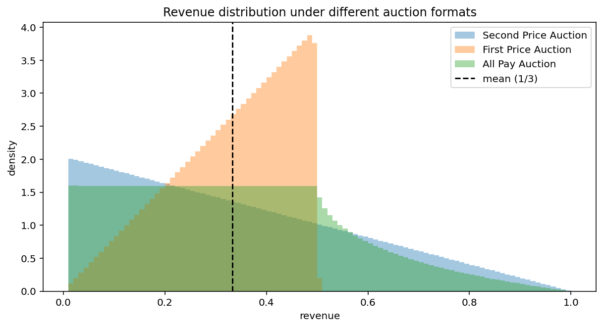
Figure 1: The revenue distribution of the Second Price, First Price, and All Pay auctions in case of two bidders with i.i.d. Uniform[0,1] value distributions. Observe that while all three formats give the same expected revenue of $\nicefrac{{1}}{{3}}$, the underlying distribution of revenue varies greatly across them.

Variance and Risk Minimization

Given different auction formats implementing the same social choice function, what auction format minimizes the variance of the revenue? When we fixed the social choice function the expectation of the revenue is fixed by the revenue equivalence theorem, but different auctions lead to different revenue distributions as we can see in Figure 1. If $R=\sum_{i}\mathcal{P}_{i}(\bm{b}(\bm{v}))$ is a random variable representing the revenue, we are interested in minimizing $\textsf{Var}(R)=\mathbb{E}[(R-\mathbb{E}[R])^{2}]=\mathbb{E}[R^{2}]-\mathbb{E}[R]^{2}$. Since $\mathbb{E}[R]^{2}$ is the same under all auction formats, we are interested in minimizing the second moment $\mathbb{E}[R^{2}]$.

More generally, we will be interested in minimizing $\mathbb{E}[f(R)]$ for a convex function $f:\mathbb{R}\rightarrow\mathbb{R}$. We will be also interested in quantifying the difference in distributions of other quantities such as $\mathbb{E}[f(U_{i})]$, $\mathbb{E}[f(U)]$ and $\mathbb{E}[f(P_{i})]$, where $U_{i}=v_{i}\cdot\mathcal{A}_{i}(\bm{b}(\bm{v}))-\mathcal{P}_{i}(\bm{b}(\bm{v}))$ is the utility of bidder $i$, $U=\sum_{i}U_{i}$ is the sum of utilities of all bidders, and $P_{i}=\mathcal{P}_{i}(\bm{b}(\bm{v}))$ is the payment of bidder $i$.

Direct Revelation Mechanisms

By the revelation principle, given an auction $\bm{\mathcal{A}}(\bm{b}),\bm{\mathcal{P}}(\bm{b})$ and a BNE $\bm{b}(\bm{v})$ it is possible to construct an alternative auction:

$$\bm{{A}}(\bm{v})=\bm{\mathcal{A}}(\bm{b}(\bm{v}))\qquad\bm{{P}}(\bm{v})=\bm{\mathcal{P}}(\bm{b}(\bm{v}))$$

that produces the exact same distribution of allocation and payments and has truthful bidding as a BNE, i.e., the auction does the bid shading on the bidders’ behalf and therefore the bidders are comfortable just submitting their true values as bids. If truthful bidding is a BNE, we say that this auction format is Bayesian Incentive Compatible (BIC). Formally, an allocation $\bm{{A}}(\bm{v})$ and payment $\bm{{P}}(\bm{v})$ are BIC if:

$$\mathbb{E}[v_{i}{A}_{i}(\bm{v})-{P}_{i}(\bm{v})\mid v_{i}]\geq\mathbb{E}[v_{i}{A}_{i}(v^{\prime}_{i},\bm{v}_{-i})-{P}_{i}(v^{\prime}_{i},\bm{v}_{-i})\mid v_{i}],\forall i,v_{i},v^{\prime}_{i}$$ (BIC)

Continuing our example of two bidders with i.i.d. uniform valuations, after substituting the equlibrium bidding functions from (2) in (1), the corresponding payment rules that make the auction BIC are:

$${P}_{i}^{\textsf{SP}}(\bm{v})=\mathcal{A}_{i}(\bm{v})\max_{j\neq i}v_{j}\qquad\qquad{P}_{i}^{\textsf{FP}}(\bm{v})=\mathcal{A}_{i}(\bm{v}/2)v_{i}/2=\mathcal{A}_{i}(\bm{v})v_{i}/2\qquad\qquad{P}_{i}^{\textsf{AP}}(\bm{v})=v_{i}^{2}/2$$ (3)

We will refer to those as the BIC implementations of SP, FP and AP respectively.

Notation

As established earlier, $(\mathcal{A},\mathcal{P})$ refer to the (potentially randomized) allocation and payment rules as a function of bids, and their BIC counterparts $({A},{P})$ refer to the same as a function of values. While the quantities $({A},{P})$ are expost, their interim counterparts are denoted by $(x,z)$. When the BIC allocation function ${A}(\bm{v})$ is deterministic, it is identical to the social choice function $A^{\text{SC}}(\bm{v})$, and when ${A}(\bm{v})$ is a random variable, $A^{\text{SC}}(\bm{v})$ is the expectation of ${A}(\bm{v})$. Given this minor difference, to avoid notational clutter, we will henceforth focus on the allocation function, even though technically ${A}(\bm{v})$ is a random variable. For instance we use the phrase “implementable allocation function” instead of “implementable social choice function”.

Winner Pays Bid Payment Rule

At the center of this paper is the notion of the winner-pays-bid (WPB) payment rule. Given an implementable allocation function $\bm{{A}}(\bm{v})$, let $x_{i}(v_{i})$ be its interim allocation and $z_{i}(v_{i})$ be the interim payment rules defined in equation (RET). We define the WPB payment rule as:

$${P}_{i}^{\textsf{WPB}}(\bm{v})=b_{i}^{\textsf{WPB}}(v_{i}){A}_{i}(\bm{v})\text{, where }b_{i}^{\textsf{WPB}}(v_{i}):=\frac{z_{i}(v_{i})}{x_{i}(v_{i})}$$ (WPB)

where we refer to $b_{i}^{\textsf{WPB}}(v_{i})$ as the bid. Note however that the WPB payment rule as defined is BIC so agents bid their true value when we use this payment rule. The function $b_{i}^{\textsf{WPB}}(v_{i})$ is a useful auxiliary notation that refers to what the bid would have been in a BNE implementation of the same allocation function ${A}(\cdot)$, where the winner pays their bid, and other agents pay zero. In other words, if we are given an allocation function ${A}(\cdot)$ and are asked to implement it as winner pays bid, we do the following.

1. In a BNE implementation, the agents submit a bid of $b_{i}^{\textsf{WPB}}(v_{i})$ and we invert the bid using the inverse of $b_{i}^{\textsf{WPB}}(\cdot)$ to get the value $v_{i}$, and implement the allocation function ${A}(\bm{v})$ on the true values obtained from inversion.

2. In a BIC implementation, agents submit their true values, and we implement the allocation function ${A}(\bm{v})$ directly on the submitted true values, and charge them a payment of $b_{i}^{\textsf{WPB}}(v_{i})$, where $b_{i}^{\textsf{WPB}}(v_{i}){A}(\bm{v})$ evaluates to evaluates to $\frac{z_{i}(v_{i})}{x_{i}(v_{i})}$.

We find the BIC version more convenient to write about because it doesn’t involve the inversion of bids to get values, even though of course there is no difference between these two versions in the distribution of outcomes and payments they produce. Here after we only focus on the BIC versions ${A}(\cdot)$ and ${P}(\cdot)$.

The astute reader might have observed that for the Winner Pays Bid payment rule to make sense, the function $\frac{z_{i}(v_{i})}{x_{i}(v_{i})}$ has to be monotonic non-decreasing. Indeed, this turns out to be the case, as formalized in the Lemma below.

Lemma 2.1.

For any implementable allocation function $\bm{{A}}(\bm{v})$ and corresponding interim allocation $x_{i}(\bm{v})$ and interim payments $z_{i}(\bm{v})$, the function $b_{i}^{\textsf{WPB}}(v_{i}):=z_{i}(v_{i})/x_{i}(v_{i})$ is monotone non-decreasing.

Proof.

We differentiate the expression for $b_{i}^{\textsf{WPB}}(v_{i})$ from the formula in equation (RET).

$$b_{i}^{\textsf{WPB}}(v_{i})=v_{i}-\int_{0}^{v_{i}}\frac{x_{i}(u)}{x_{i}(v_{i})}du$$

$$(b_{i}^{\textsf{WPB}})^{\prime}(v_{i})=1-\frac{x_{i}(v_{i})}{x_{i}(v_{i})}-\int_{0}^{v_{i}}\frac{-x^{\prime}_{i}(v_{i})x_{i}(u)}{x_{i}(v_{i})^{2}}du=\int_{0}^{v_{i}}\frac{x^{\prime}_{i}(v_{i})x_{i}(u)}{x_{i}(v_{i})^{2}}du\geq 0.$$

The inequality holds because $x_{i}(\cdot)$ is monotone non-decreasing for any implementable $\bm{{A}}(\cdot)$. ∎

Lemma 2.1 says that regardless of whether the value distributions across bidders is independent or correlated, symmetric or asymmetric, any implementable allocation function can be implemented with a Winner Pays Bid payment rule.

Jensen’s inequality

We will use the fact that for a convex function $f$ and a random variable $Y$, it holds that $\mathbb{E}[f(Y)]\geq f(\mathbb{E}[Y])$ and that it holds with equality whenever there is a constant $y$ such that $Y=y$ almost surely.

3 Risk-Minimizing Ex-post IR mechanisms

We saw in the the running example in Section 2 that even when we fix the allocation function, there is a great deal of flexibility in defining an auction rule that implements that allocation function in a BNE. For example, any of the payment rules in equation (1) leads to a BNE implementation of the efficient allocation rule. Even when we restrict our attention to BIC mechanisms (which can be done without loss of generality by the revelation principle), the flexibility still remains. Observe that any of the payment rules in equation (3) coupled with the efficient allocation rule leads to a BIC auction.

The main question we ask is: Given a fixed allocation function, among all the payments that implement it, what is the payment function that minimizes risk associated with the total revenue $\mathbb{E}[f(R)]$ for a given convex function, $f$.

We initially restrict our attention to (BIC) ex-post IR mechanisms, i.e., mechanisms for which $v_{i}{A}_{i}(\bm{v})-{P}_{i}(\bm{v})\geq 0$ for all $\bm{v}$. This includes mechanisms like (the BIC implementation of) SP and FP but excludes AP. In the next section we will revisit this problem without the restriction to ex-post IR. The important property we will exploit from ex-post IR mechanism is that bidders that don’t win pay zero, i.e.: ${P}_{i}(\bm{v})=0$ whenever ${A}_{i}(\bm{v})=0$.

Theorem 3.1.

Given any prior on the buyers’ private valuations $\mathcal{D}$ and any implementable allocation function $\bm{{A}}(\bm{v})$, among all ex-post IR payment rules that implement $\bm{{A}}(\bm{v})$, the winner-pays-bid payment rule minimizes the expected risk $\mathbb{E}[f(R)]$ for any convex function $f$, where $R=\sum_{i}{P}_{i}(\bm{v})$ is the random variable corresponding to the total revenue.

Proof.

Given the revelation principle, it is without loss of generality to focus on BIC mechanisms. Let $\bm{{P}}(\bm{v})$ be any payment rule implements $\bm{{A}}(\bm{v})$ and let ${P}^{\textsf{WPB}}(\bm{v})$ be the winner-pays-bid payment rule associated with $\bm{{A}}(\bm{v})$. We know by (RET) that $\mathbb{E}[\sum_{j}{P}_{j}(\bm{v})]=\mathbb{E}[\sum_{j}{P}^{\textsf{WPB}}_{j}(\bm{v})]$. We want to show that

$$\textstyle\mathbb{E}[f(\sum_{j}{P}_{j}(\bm{v}))]\geq\mathbb{E}[f(\sum_{j}{P}^{\textsf{WPB}}_{j}(\bm{v}))]$$

We will focus on one bidder at a time and show the inequality above conditioned on $i$ having value $v_{i}$ and being the winner (${A}_{i}(\bm{v})=1$). By ex-post IR, we know that in that case: $\sum_{j}{P}_{j}(\bm{v})={P}_{i}(\bm{v})$. Hence we have:

$$\textstyle\mathbb{E}[f(\sum_{j}{P}_{j}(\bm{v}))\mid v_{i},{A}_{i}(\bm{v})=1] =\mathbb{E}[f({P}_{i}(\bm{v}))\mid v_{i},{A}_{i}(\bm{v})=1]$$

$$\geq f(\mathbb{E}[{P}_{i}(v)\mid v_{i},{A}_{i}(\bm{v})=1])$$

Where the first step is because of restriction to ex-post IR payment rules, and the second step is by Jensen’s inequality. Now we have observe that:

$$\mathbb{E}[{P}_{i}(\bm{v})\mid v_{i},{A}_{i}(\bm{v})=1]=\frac{\mathbb{E}[{P}_{i}(\bm{v}){A}_{i}(\bm{v})\mid v_{i}]}{\mathbb{P}[{A}_{i}(\bm{v})=1\mid v_{i}]}=\frac{z_{i}(v_{i})}{x_{i}(v_{i})}=\mathbb{E}[{P}_{i}^{\textsf{WPB}}(v_{i})\mid v_{i},{A}_{i}(\bm{v})=1]$$

where the second equality again relies on ex-post IR, since ${P}_{i}(\bm{v}){A}_{i}(\bm{v})={P}_{i}(\bm{v})$. Plugging that in the previous equation we have:

$$\textstyle\mathbb{E}[f(\sum_{j}{P}_{j}(\bm{v}))\mid v_{i},{A}_{i}(\bm{v})=1] \geq f(\mathbb{E}[{P}_{i}^{\textsf{WPB}}(\bm{v})\mid v_{i},{A}_{i}(\bm{v})=1])$$

$$=\mathbb{E}[f({P}_{i}^{\textsf{WPB}}(\bm{v}))\mid v_{i},{A}_{i}(\bm{v})=1])$$

$$=\textstyle\mathbb{E}[f(\sum_{j}{P}_{j}^{\textsf{WPB}}(\bm{v}))\mid v_{i},{A}_{i}(\bm{v})=1])$$

The equality in the second line is the case where Jensen’s inequality holds with equality since ${P}_{i}^{\textsf{WPB}}(\bm{v})$ is completely determined when conditioned on $v_{i},{A}_{i}(\bm{v})=1$. Finally the last equality is due to the fact that only the winner pays in WPB.

Taking expectations over $v_{i},{A}_{i}(\bm{v})=1$, summing over all bidders and applying the law of total expectation concludes the proof. ∎

Corollary 3.2.

In the setting of Theorem 3.1, WPB minimizes the variance $\mathsf{Var}(R)=\mathbb{E}[(R-\mathbb{E}[R])^{2}]$ among ex-post IR mechanisms.

Proof.

We can decompose $\mathsf{Var}(R)=\mathbb{E}[R^{2}]-\mathbb{E}[R]^{2}$. By the revenue equivalence theorem (RET), the second term is the same across all payment rules. By the previous theorem with $f(x)=x^{2}$, the first term is minimized for WPB. ∎

Corollary 3.3.

In the setting of Theorem 3.1, WPB minimizes the risk of each individual bidder’s payment $\mathbb{E}[f(P_{i})]$, the risk of each individual bidder’s $\mathbb{E}[f(U_{i})]$ and the risk of the sum of all the bidders’ utilities $\mathbb{E}[f(U)]$ among all ex-post IR payment rules.

Proof.

The proof that WPB minimizes $\mathbb{E}[f(P_{i})]$ is direct from the proof of Theorem 3.1. The argument for utility and sum of utilities follows exactly the same proof format by observing that: (i) only the winner has non-zero utility; (ii) in WPB, the utility of an agent is completely determined when conditioned on $v_{i}$ and ${A}_{i}(\bm{v})=1$. With those observations the exact same argument carries through. ∎

4 Risk-Minimization Beyond Ex-post IR

The proof of Theorem 3.1 crucially relies on ex-post IR on two different points, but interestingly, the proof makes no requirement about the distribution of values $\mathcal{D}$. In particular, it allows it to be both asymmetric and correlated.

In this section, we will drop the ex-post IR requirement and only require interim IR, i.e., $\mathbb{E}[v_{i}{A}_{i}(\bm{v})-{P}_{i}(\bm{v})\mid v_{i}]\geq 0$. This will allow us to analyze auctions like all-pay (AP). All-pay is a natural candidate for a variance minimizing auction since it minimizes the the variance of the payment of each individual agent:

Lemma 4.1.

Given any prior on the buyers’ private valuations $\mathcal{D}$ and any implementable allocation function $\bm{{A}}(\bm{v})$, among all payment rules that implement $\bm{{A}}(\bm{v})$, the all-pay rule ${P}^{\textsf{AP}}_{i}(\bm{v})=z_{i}(v_{i})$ minimizes the risk $\mathbb{E}[f(P_{i})]$ where $f$ is any convex function and $P_{i}(\bm{v})$ is the random variable corresponding to the payment of agent $i$.

Proof.

Given any payment rule ${P}(\bm{v})$ implementing the given allocation function ${A}(v)$ and any convex function $f$ we want to show that $\mathbb{E}[f({P}_{i}(\bm{v}))]\geq\mathbb{E}[f({P}_{i}^{\textsf{AP}}(\bm{v}))]$. The proof follows the same pattern as the proof of Theorem 3.1 but without conditioning on the winning bidder. We observe that:

$$\mathbb{E}[f({P}_{i}(\bm{v}))\mid v_{i}]\geq f(\mathbb{E}[{P}_{i}(\bm{v})\mid v_{i}])=f(\mathbb{E}[{P}_{i}^{\textsf{AP}}(\bm{v})\mid v_{i}])=\mathbb{E}[f({P}_{i}^{\textsf{AP}}(\bm{v}))\mid v_{i}]$$

where the first inequality is Jensen’s inequality, the subsequent equality is due to the revenue equivalence theorem (RET) and the final equality is due to the fact that ${P}_{i}^{\textsf{AP}}(\bm{v})$ is completely determined when conditioned on the type $v_{i}$ and hence Jensen’s inequality holds with equality. ∎

While AP minimizes the risk (and variance) of each individual payments, it doesn’t minimize variance for the revenue. The reason is that the the second moment of the revenue is:

$$\textstyle\mathbb{E}[(\sum_{i}{P}_{i}(\bm{v}))^{2}]=\sum_{i}\mathbb{E}[{P}_{i}(\bm{v})^{2}]+2\sum_{i\neq j}\mathbb{E}[{P}_{i}(\bm{v}){P}_{j}(\bm{v})]$$

The first term corresponds to the second moment of each individual bidder. For ex-post IR auctions, since only the winner pays, the second term disappears. For AP auctions (and non ex-post IR auction more generally) the second term is not identically zero, and, in fact, tends to dominate the variance.

4.1 Symmetric Settings

The situation for non ex-post IR auctions is more nuanced and depends on how symmetric the setting is. We will assume that the allocation rule $\bm{{A}}(\bm{v})$ is the efficient allocation (with any tie breaking rule). We say that a distribution $\mathcal{D}$ is symmetric for the efficient allocation whenever the distribution of values is such that the the interim allocation functions are the same for every bidder:

$$x_{i}(s)=x_{j}(s),\forall s,i\neq j$$

This happens, for example, when the distribution $\mathcal{D}$ is exchangeable (but not necessarily independent).

Lemma 4.2.

For the efficient allocation $\bm{{A}}(\bm{v})$ coupled with the WPB payment function in a symmetric setting, we can write the revenue as:

$$\textstyle\sum_{i}{P}_{i}^{\textsf{WPB}}(\bm{v})=\max_{i}b^{\textsf{WPB}}(v_{i})$$

where $b^{\textsf{WPB}}(v_{i}):=z_{i}(v_{i})/x_{i}(v_{i})$ (we drop the subscript $i$ from $b^{\textsf{WPB}}$ since the $b^{\textsf{WPB}}$ is the same across all bidders in a symmetric setting).

Proof.

Since the allocation is efficient, then the winner is the agent with the highest value, therefore:

$$\textstyle\sum_{i}{P}_{i}^{\textsf{WPB}}(\bm{v})=b^{\textsf{WPB}}(\max_{j}v_{j})=\max_{i}b^{\textsf{WPB}}(v_{i})$$

where the second equality follows from the monotonicity of $b^{\textsf{WPB}}$ established in Lemma 2.1. ∎

Theorem 4.3.

Given the efficient allocation $\bm{{A}}(\bm{v})$ and a symmetric prior $\mathcal{D}$, then among all payment rules that implement the efficient allocation, the winner-pays-bid payment rule minimizes the risk $\mathbb{E}[f(R)]$ where $f$ is any convex function and $R=\sum_{i}{P}_{i}(\bm{v})$ is the random variable corresponding to the total revenue.

Proof.

It is again without loss of generality to focus on BIC mechanisms. We will show that given any payment rule ${P}_{i}(\bm{v})$ that implements the efficient allocation we have $\mathbb{E}[f(\sum_{j}{P}_{J}(\bm{v}))]\geq\mathbb{E}[f(\sum_{j}{P}_{J}^{\textsf{WPB}}(\bm{v}))]$. We start by applying convexity:

$$\textstyle f(\sum_{j}{P}_{j}(\bm{v}))\geq f(\sum_{j}{P}_{j}^{\textsf{WPB}}(\bm{v}))+f^{\prime}(\sum_{j}{P}_{j}^{\textsf{WPB}}(\bm{v}))\cdot(\sum_{j}{P}_{j}(\bm{v})-\sum_{j}{P}_{j}^{\textsf{WPB}}(\bm{v}))$$

Taking expectations over the expression above, we observe that it is enough to establish that:

$$\textstyle\mathbb{E}[f^{\prime}(\sum_{j}{P}_{j}^{\textsf{WPB}}(\bm{v}))\cdot(\sum_{i}{P}_{i}(\bm{v})-\sum_{i}{P}_{i}^{\textsf{WPB}}(\bm{v}))]\geq 0$$ (4)

In order to show equation (4), we will start by using Lemma 4.2 to decompose the derivative term for each bidder $i$ as follows:

$$\textstyle f^{\prime}(\sum_{j}{P}_{j}^{\textsf{WPB}}(\bm{v}))=\lambda_{i}(v_{i})+\mu_{i}(\bm{v})$$ (5)

for

$$\lambda_{i}(v_{i})=f^{\prime}(b^{\textsf{WPB}}(v_{i}))\quad\text{and}\quad\mu_{i}(\bm{v})=f^{\prime}(\max_{j}b^{\textsf{WPB}}(v_{j}))-f^{\prime}(b^{\textsf{WPB}}(v_{i}))$$

Now, we can re-write the left hand side of equation (4) as:

$$\textstyle\mathbb{E}[f^{\prime}(\sum_{j}{P}_{j}^{\textsf{WPB}}(\bm{v}))\cdot(\sum_{i}{P}_{i}(v)-\sum_{i}{P}_{i}^{\textsf{WPB}}(\bm{v}))]$$

$$\qquad=\textstyle\sum_{i}\mathbb{E}[f^{\prime}(\sum_{j}{P}_{j}^{\textsf{WPB}}(\bm{v}))({P}_{i}(\bm{v})-{P}_{i}^{\textsf{WPB}}(\bm{v}))]$$

$$\qquad=\textstyle\sum_{i}\mathbb{E}[(\lambda_{i}(v_{i})+\mu_{i}(\bm{v}))({P}_{i}(\bm{v})-{P}_{i}^{\textsf{WPB}}(\bm{v}))]$$

$$\qquad=\textstyle\sum_{i}\mathbb{E}[\lambda_{i}(v_{i})({P}_{i}(\bm{v})-{P}_{i}^{\textsf{WPB}}(\bm{v}))]+\sum_{i}\mathbb{E}[\mu_{i}(\bm{v})({P}_{i}(\bm{v})-{P}_{i}^{\textsf{WPB}}(\bm{v}))]$$

where the first and last equalities are re-arrangement of terms and the second equality is the revenue decomposition in equation (5). We conclude the proof by showing that each of the terms in the last expression is non-negative.

For the first term, we observe that $\lambda_{i}(v_{i})$ depends only on $v_{i}$, so we can apply the revenue equivalence theorem (RET) as follows:

$$\mathbb{E}[\lambda_{i}(v_{i})({P}_{i}(\bm{v})-{P}_{i}^{\textsf{WPB}}(\bm{v}))]=\mathbb{E}_{v_{i}}[\lambda_{i}(v_{i})\cdot\mathbb{E}[{P}_{i}(\bm{v})-{P}_{i}^{\textsf{WPB}}(\bm{v})\mid v_{i}]]=0$$

since $\mathbb{E}[{P}_{i}(\bm{v})\mid v_{i}]=\mathbb{E}[{P}_{i}^{\textsf{WPB}}(\bm{v})\mid v_{i}]$.

For the second term we observe that $\mu_{i}(\bm{v})\geq 0$, since by convexity $f^{\prime}$ is monotone non-decreasing. Also, $\mu_{i}(\bm{v})=0$ whenever $i$ is the winner. Since ${P}_{i}^{\textsf{WPB}}(\bm{v})=0$ whenever $i$ doesn’t win, it follows that:

$$\mu_{i}(\bm{v}){P}_{i}^{\textsf{WPB}}(\bm{v})=0.$$

Hence we can write the second term as:

$$\mathbb{E}[\mu_{i}(\bm{v})({P}_{i}(\bm{v})-{P}_{i}^{\textsf{WPB}}(\bm{v}))]=\mathbb{E}[\mu_{i}(\bm{v}){P}_{i}(\bm{v})]\geq 0$$

which concludes the proof. ∎

Corollary 4.4.

Let $\bm{{A}}(\bm{v})$ be the allocation that selects the highest bidder if it is above a fixed reserve price $r$ otherwise selects no one. For a symmetric prior, the winner-pays-bid payment rule minimizes risk $\mathbb{E}[f(R)]$ for any convex function $f$.

Proof.

Same as the previous theorem except that we re-define $b^{\textsf{WPB}}(v_{i})$ such that it is zero for $v_{i}<r$. ∎

4.2 Asymmetric Settings

For asymmetric settings with interim IR payments, the winner-pays-bid payment rule is no longer guaranteed to minimize the revenue variance. We consider an example with two independent bidders with c.d.f. $F_{1}(v_{1})=v_{1}$ and $F_{2}(v_{2})=v_{2}^{2}$. In the efficient allocation, the interim allocation probabilities are: $x_{1}(v_{1})=F_{2}(v_{1})=v_{1}^{2}$ and $x_{2}(v_{2})=F_{1}(v_{2})=v_{2}$ and the interim payment are given by the Myerson integral in equation (RET):

$$z_{1}(v_{1})=\int_{0}^{v_{1}}(x_{1}(v_{1})-x_{1}(u))du=\frac{2}{3}v_{1}^{3}\qquad z_{2}(v_{2})=\int_{0}^{v_{2}}(x_{2}(v_{2})-x_{2}(u))du=\frac{1}{2}v_{2}^{2}$$

Now, the winner pays bid auction charges $b_{1}(v_{1})=z_{1}(v_{1})/x_{1}(v_{1})$ to agent $1$ whenever $v_{1}\geq v_{2}$ and $b_{2}(v_{2})=z_{2}(v_{2})/x_{2}(v_{2})$ to agent $2$ whenever $v_{2}>v_{1}$. Hence we must have: $b_{1}(v_{1})=2v_{1}/3$ and $b_{2}(v_{2})=v_{2}/2$. Using this, we can compute the second moment of the revenue of WPB:

$$\int_{0}^{1}f_{1}(v)x_{1}(v)b_{1}(v)^{2}dv+\int_{0}^{1}f_{2}(v)x_{2}(v)b_{2}(v)^{2}dv\approx 0.188$$

Now, we describe a payment rule that is a BIC-implementation of the optimal allocation and has strictly smaller variance. Consider the payments:

$${P}_{1}^{*}(v_{1},v_{2})=\pi_{1}(v_{1})\cdot\mathbf{1}\{h(v_{1})\geq v_{2}\}\qquad{P}_{2}^{*}(v_{1},v_{2})=\pi_{2}(v_{2})\cdot\mathbf{1}\{v_{2}>h(v_{1})\}$$

for functions:

$$h(u)=u\left(\frac{4}{3}\right)^{1/4}\qquad\pi_{1}(v_{1})=\left\{\begin{aligned} &v_{1}/\sqrt{3},&&\text{for }v_{1}\leq(3/4)^{1/4}\\ &2v_{1}^{3}/3,&&\text{for }v_{1}>(3/4)^{1/4}\end{aligned}\right.\qquad\pi_{2}(v_{2})=\frac{v_{2}}{2}\left(\frac{4}{3}\right)^{1/4}$$

The auction is depicted in Figure 2. It has the non-standard feature that in a small region (labelled B in the figure), bidder 2 gets the item but bidder 1 pays $\pi_{1}(v_{1})$. First, we can check that this payment rule coupled with the efficient allocation in a BIC auction by checking that the revenue equivalence holds:

$$\int_{0}^{1}f_{2}(v_{2}){P}_{1}^{*}(v_{1},v_{2})dv_{2}=z_{1}(v_{1})\qquad\int_{0}^{1}f_{1}(v_{1}){P}_{2}^{*}(v_{1},v_{2})dv_{1}=z_{2}(v_{2})$$

And we can compute its second moment as:

$$\int_{0}^{h^{-1}(1)}f_{1}(v_{1})F_{2}(h(v_{1}))\pi_{1}(v_{1})^{2}dv_{1}+\int_{h^{-1}(1)}^{1}f_{1}(v_{1})z_{1}(v_{1})^{2}dv_{1}$$

$$\quad+\int_{0}^{1}f_{2}(v_{2})F_{1}(h^{-1}(v_{2}))\pi_{2}(v_{2})^{2}dv_{2}\approx 0.186$$

Figure 2: In the efficient mechanism that minimizes revenue variance for $2$ asymmetric bidders with pdf $F_{1}(v_{1})=v_{1}$ and $F_{2}(v_{2})=v_{2}^{2}$, we allocate to bidder $1$ in regions A and to bidder $2$ in regions B+C, but agent $1$ pays in regions A+B while bidder $2$ pays in regions B+C. Hence, in the shaded region, bidder $2$ is allocated but bidder $1$ pays.

The intuition why WPB is not optimal for asymmetric valuation is that $b_{1}(u)>b_{2}(u)$ so it no longer holds that ${P}_{1}(v_{1},v_{2})+{P}_{2}(v_{1},v_{2})=\max(b_{1}(v_{1}),b_{2}(v_{2}))$, which is what is driving optimality in Theorem 4.3. A solution is to increase the region where bidder $1$ pays so that we can spread their payments along a larger region. With the new design, we have that ${P}_{1}^{*}(v_{1},v_{2})+{P}_{2}^{*}(v_{1},v_{2})=\max(\pi_{1}(v_{1}),\pi_{2}(v_{2}))$. This implies that $\bm{{P}}^{*}$ is actually the variance minimizing payment rule for this environment. More generally we can prove that:

Theorem 4.5 (Optimality Condition).

Consider any allocation function $\bm{{A}}(\bm{v})$ and any prior distribution $\mathcal{D}$. Given functions $\pi_{i}(v_{i})$, let $\bm{{P}}^{*}(\bm{v})$ be the payment rule where the agent with largest $\pi_{i}(v_{i})$ pays $\pi_{i}(v_{i})$ (breaking ties arbitrarly) and the remaining agents pay zero. Then if $\bm{{P}}^{*}$ satisfies the revenue equivalence theorem (equation (RET)) then for any convex function $f$ then $\mathbb{E}[f(\sum_{i}{P}_{i}^{*}(\bm{v}))]\leq\mathbb{E}[f(\sum_{i}{P}_{i}(\bm{v}))]$ for any payment rule $\bm{{P}}(\bm{v})$ implementing allocation $\bm{{A}}(\bm{v})$.

Proof.

Let $\bm{{P}}(\bm{v})$ be any payment rule implementing the allocation function and let $\bm{{P}}^{*}(\bm{v})$ be a payment rule satisfying the optimality conditions in the theorem statement. To show that $\mathbb{E}[f(\sum_{i}{P}_{i}^{*}(\bm{v}))]\leq\mathbb{E}[f(\sum_{i}{P}_{i}(\bm{v}))]$, it is enough to show that $\mathbb{E}[f^{\prime}(\sum_{i}{P}_{i}^{*}(\bm{v}))(\sum_{i}{P}_{i}(\bm{v})-\sum_{i}{P}_{i}^{*}(\bm{v}))]\geq 0$ by the argument in the proof of Theorem 4.3. We decompose the revenue as follows:

$$\textstyle f^{\prime}(\sum_{i}{P}_{i}^{*}(\bm{v}))=\lambda_{i}(v_{i})+\mu_{i}(\bm{v})$$

where:

$$\lambda_{i}(v_{i})=f^{\prime}(\pi_{i}(v_{i}))\qquad\mu_{i}(\bm{v})=f^{\prime}(\max_{j}\pi_{j}(v_{j}))-f^{\prime}(\pi_{i}(v_{i}))$$

As in the proof of Theorem 4.3, we can write:

$$\textstyle\mathbb{E}[f^{\prime}(\sum_{i}{P}_{i}^{*}(\bm{v}))(\sum_{i}{P}_{i}(\bm{v})-\sum_{i}{P}_{i}^{*}(\bm{v}))]=\textstyle\sum_{i}\mathbb{E}[\lambda_{i}(v_{i})({P}_{i}(\bm{v})-{P}_{i}^{*}(\bm{v}))]+\sum_{i}\mathbb{E}[\mu_{i}(\bm{v})({P}_{i}(\bm{v})-{P}_{i}^{*}(\bm{v}))]$$

The first term is zero by the revenue equivalence theorem and since $\mu_{i}(\bm{v})=0$ whenever ${P}^{*}_{i}(\bm{v})>0$ we have $\mu_{i}(\bm{v}){P}^{*}_{i}(\bm{v})=0$. The second term is therefore: $\sum_{i}\mathbb{E}[\mu_{i}(\bm{v}){P}_{i}(\bm{v})]\geq 0$. ∎

4.3 Negative Payments

So far we assumed throughout the paper that payments are non-negative ${P}_{i}(\bm{v})\geq 0$, i.e., transfers are only allowed from the bidders to the auctioneer. If we drop this restriction but still enforce interim IR, then it is possible to construct an auction where the variance of the revenue is zero whenever the values are independent.

Theorem 4.6.

Given a prior $\mathcal{D}$ that is independent across buyers’ private valuation and any implementable allocation function $\bm{{A}}(\bm{v})$, then there exists a payment rule $\bm{{P}}(\bm{v})$ with possibly negative payments that is interim IR, BIC and the variance of the total revenue $R=\sum_{i}{P}_{i}(\bm{v})$ is zero.

Proof.

For each bidder $i$, let $z_{i}(v_{i})$ be the interim payments in equation (RET). Also define $\bar{z}_{i}=\mathbb{E}[z_{i}(v_{i})]$ as the average payment of bidder $i$. Now, define:

$$\textstyle{P}_{i}(\bm{v})=z_{i}(v_{i})+\frac{1}{n-1}\sum_{j\neq i}(\bar{z}_{j}-z_{j}(v_{j}))$$

We first observe that $\mathbb{E}[{P}_{i}(\bm{v})\mid v_{i}]=z_{i}(v_{i})$, so the payment rule implements the allocation rule $a(v)$. Now, observe that:

$$\textstyle\sum_{i}{P}_{i}(\bm{v})=\sum_{i}(z_{i}(\bm{v})+\bar{z}_{i}-z_{i}(\bm{v}))=\sum_{i}\bar{z}_{i}$$

Hence the total revenue is constant across all vectors of types. ∎

References

- [1] Bergemann, D., and Horner, J. Should auctions be transparent? Cowles Foundation Discussion Papers 1764R2, Cowles Foundation for Research in Economics, Yale University, 2017.
- [2] Chawla, S., Goldner, K., Miller, J. B., and Pountourakis, E. Revenue maximization with an uncertainty-averse buyer, 2018.
- [3] Harris, M., and Raviv, A. Allocation mechanisms and the design of auctions. Econometrica 49, 6 (1981), 1477–99.
- [4] Holt, C. Competitive bidding for contracts under alternative auction procedures. Journal of Political Economy 88, 3 (1980), 433–45.
- [5] Krishna, V. Auction Theory, 1 ed. Elsevier, 2002.
- [6] Lucking-Reiley, D. Vickrey auctions in practice: From nineteenth-century philately to twenty-first-century e-commerce. Journal of Economic Perspectives 14, 3 (September 2000), 183–192.
- [7] Maskin, E., and Riley, J. Optimal auctions with risk-averse buyers. Econometrica 52, 6 (1984), 1473–1518.
- [8] Matthews, S. A. Selling to risk averse buyers with unobservable tastes. Journal of Economic Theory 30, 2 (1983), 370–400.
- [9] Milgrom, P., and Weber, R. A theory of auctions and competitive bidding. Econometrica 50, 5 (1982), 1089–1122.
- [10] Milgrom, P. R. Auction theory. Econometric Society Monographs. Cambridge University Press, 1987, p. 1–32.
- [11] Moore, J. Global incentive constraints in auction design. Econometrica 52, 6 (1984), 1523–1535.
- [12] Myerson, R. B. Optimal auction design. Math. Oper. Res. 6, 1 (feb 1981), 58–73.
- [13] Pesendorfer, M. A study of collusion in first-price auctions. Review of Economic Studies 67, 3 (2000), 381–411.
- [14] Riley, J., and Samuelson, W. F. Optimal auctions. American Economic Review 71, 3 (1981), 381–92.
- [15] Sundararajan, M., and Yan, Q. Robust mechanisms for risk-averse sellers. Games Econ. Behav. 124 (2020), 644–658.
- [16] Vickrey, W. Counterspeculation, auctions and sealed tenders. Journal of Finance 16, 1 (1961), 8–37.