Dark Matter Line Searches with the Cherenkov Telescope Array

Abstract

Monochromatic gamma-ray signals constitute a potential smoking gun signature for annihilating or decaying dark matter particles that could relatively easily be distinguished from astrophysical or instrumental backgrounds. We provide an updated assessment of the sensitivity of the Cherenkov Telescope Array (CTA) to such signals, based on observations of the Galactic centre region as well as of selected dwarf spheroidal galaxies. We find that current limits and detection prospects for dark matter masses above 300 GeV will be significantly improved, by up to an order of magnitude in the multi-TeV range. This demonstrates that CTA will set a new standard for gamma-ray astronomy also in this respect, as the world’s largest and most sensitive high-energy gamma-ray observatory, in particular due to its exquisite energy resolution at TeV energies and the adopted observational strategy focussing on regions with large dark matter densities. Throughout our analysis, we use up-to-date instrument response functions, and we thoroughly model the effect of instrumental systematic uncertainties in our statistical treatment. We further present results for other potential signatures with sharp spectral features, e.g. box-shaped spectra, that would likewise very clearly point to a particle dark matter origin.

1 Introduction

The nature of the cosmological dark matter (DM), contributing about $26\,\%$ to the total energy content of the universe [1], remains unknown. The most often discussed explanation is that of a hypothetical elementary particle, and a plethora of viable DM candidates of this type has been suggested in the literature [2, 3, 4]. Gamma rays produced from the annihilation or decay of these particles may provide a promising way to test the particle hypothesis of DM [5].

The Cherenkov Telecope Array Observatory (CTAO) [6], whose construction is starting, will be in an excellent position to perform such an indirect search for DM. One of the reasons is the estimated unprecedented angular resolution and sensitivity of this observatory, for gamma-ray energies from below 100 GeV to at least several tens of TeV. As recently demonstrated [7], in particular, these properties imply the exciting prospect that the Cherenkov Telecope Array (CTA) may be able to robustly probe thermally produced weakly interacting massive particles (WIMPs), i.e. the most prominently discussed type of DM candidates (for earlier work arriving at similar conclusions, see also Refs. [8, 9, 10, 11, 12]). Here we focus instead on a different property of CTAO, namely its very good energy resolution. As we show here, this may help to single out characteristic spectral features expected in several DM models – which, in the case of a detection, would allow a much more robust signal claim because the discrimination against astrophysical and instrumental backgrounds would be significantly easier than for the generic WIMP signals studied in Ref. [7].

Examples for such smoking gun signatures of DM include monochromatic gamma-ray ‘lines’ [13, 14, 15], box-shaped signals [16] and other strongly enhanced spectral features at energies close to the DM particle’s mass [17]. In fact, the details of the spectrum allow to not only discriminate DM from background components, but can also provide valuable insights about the underlying particle physics model [5]. On the other hand, such features in the gamma-ray spectra from DM typically appear at smaller rates than the generic spectra expected from the simplest WIMP models (though, as discussed explicitly further down, prominent counterexamples exist). In this sense, those generic spectra typically have a significantly better DM constraining potential, while distinct spectral features provide a very promising discovery channel (for DM models that exhibit such spectra).

This difference is also reflected in the analysis methods that are most suitable to identify a potential DM signal. For the continuum signals expected from generic WIMP models the spectral information is less important than the angular information, motivating the use of detailed spatial templates for the DM and the various background components [7]. Clearly, this approach is limited by the precision to which in particular the different background components can be modelled. For (almost) monochromatic signals, on the other hand, the exact knowledge of the spatial morphology of the background is less crucial. In fact, the analysis also becomes to some degree independent of the energy dependence of the background, as long as it varies much less strongly with energy than the signal. It is worth noting that this generic property of spectral ‘line searches’ has been successfully employed not only in the context of DM searches [18, 19, 20, 21, 22, 23, 24] but also, e.g., in the discovery of the standard model Higgs boson [25, 26].

In this article we complement the DM analysis of Ref. [7] by estimating the sensitivity of CTAO to monochromatic and similar ‘smoking gun’ signals, highly localized in energy. We adopt up-to-date background models and the current best estimates for the expected instrument performance, using a binned profile likelihood ratio test inside a sliding energy window in the range from 200 GeV to 30 TeV. For this analysis approach, we pay special attention to quantify the impact of systematic uncertainties in the event reconstruction. We discuss prospects both for observations of the Galactic Centre (GC) region, where the DM density and hence the signal strength is expected to be largest, and for stacking observations of dwarf spheroidal galaxies (dSPhs) where astrophysical gamma-ray backgrounds can largely be neglected at the energies of interest here. For previous work estimating the CTA prospects to observe sharp spectral features, see Refs. [27, 28, 29, 30, 31].

This article is organized as follows. In Section 2 we give a brief introduction to CTAO and its expected performance. Section 3 introduces in more detail the characteristic spectral features that we focus our analysis on, along with a motivation from the underlying DM models. We discuss the specifics of the target regions of this sensitivity analysis in Section 4, both with respect to the modelling of the astrophysical emission components and with respect to the expected DM distribution. In Section 5 we provide details about the analysis techniques adopted in this work. We present our results in Section 6, and discuss them further in Section 7. Our final conclusions are given in Section 8. In Appendix A we provide further details about the statistical analysis method that we adopted.

2 The Cherenkov Telescope Array Observatory

Ground-based gamma-ray astronomy started in the 1980s when the Whipple telescope [32] demonstrated the feasibility of the imaging atmospheric Cherenkov light technique. The field of ground-based observations of very high-energy gamma rays then quickly grew to one of the main contributors to modern-day astroparticle physics, expanding to include also water Cherenkov techniques (as pioneered, starting from 1999, by Milagro [33]).

Imaging Atmospheric Cherenkov Telescopes (IACTs) operate by detecting extended showers of Cherenkov light that are produced in the atmosphere due to cascades of relativistic particles resulting from incident high-energy cosmic ray (CR) particles and gamma rays [34]. Due to telescope and camera architecture, the field of view (FoV) of current IACTs is generally limited to several degrees. Currently operating IACT systems are H.E.S.S (5 telescopes, Namibia) [35], VERITAS (4 telescopes, Arizona) [36], and MAGIC (2 telescopes, La Palma) [37]. Having a larger number of telescopes is beneficial, as it allows tracking the shower from multiple angles, and therefore improving the reconstruction of the arrival direction and energy of the event. The discrimination between CR proton and gamma-ray induced events is possible via the image shape, based on Monte Carlo (MC) simulations, which however cannot discriminate electrons and gamma rays. Since CRs arriving at the top of the atmosphere are dominated by protons, with gamma rays only making up a tiny fraction (e.g. $10^{-4}$ of the proton flux at 1 TeV), large backgrounds due to misidentified charged CRs often present an unavoidable consequence for ground-based detection. Next generation water Cherenkov facilities like SWGO may have comparable sensitivity in the multi TeV range [38, 39]; their expectedly worse energy resolution, however, makes them less competitive to search for the kind of monochromatic spectral features that we will focus on in our analysis.

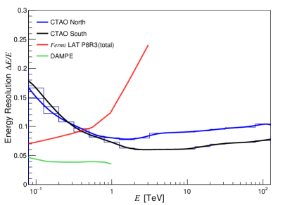
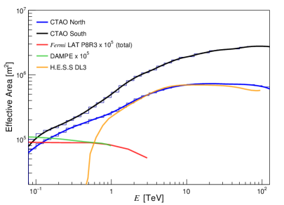
Figure 1: Left panel. The expected energy resolution of CTAO as a function of (true) energy for the northern (blue) and southern (black) array, obtained as linear interpolation of the histograms provided with the IRF (indicated with thinner lines; cf. footnote 1). Here the energy resolution $\Delta E$ is defined such that $68\%$ of the reconstructed gamma-rays will have a true energy within $\Delta E$. For comparison, we also show in red the energy resolution for Fermi-LAT Pass 8 Release 3 SOURCE V3 (total) [40] and in green that for DAMPE [41]. Right panel. Effective area of the two site locations as a function of energy. The thick solid lines are based on a Gaussian smoothing of width $\Delta E$, as used in our analysis. In addition, we show the effective areas for Fermi (red), DAMPE (green) and H.E.S.S. Data Level 3 (DL3) [42] (orange).

CTAO [43] is the next-generation ground-based gamma-ray instrument facility. Its construction is already starting, and large-scale telescope production is expected to begin in 2025. The goal of CTA (for the so-called ‘Omega’ configuration) is to build about 100 IACTs of three different sizes and distribute them among two locations, one for each hemisphere: Paranal in Chile for the southern hemisphere, and La Palma in Spain for the northern. The southern hemisphere array will consist of telescopes covering the entire energy range of CTAO; LSTs (Large-Sized Telescopes) for the $20\!-\!150$ GeV range, MSTs (Medium-Sized Telescopes) for the $150$ GeV to $5$ TeV range and finally SSTs (Small-Sized Telescope) for energies from $5$ TeV to $300$ TeV and more. The northern hemisphere array will instead be more limited in size, and will focus on energies from 20 GeV to 20 TeV. In a first stage of CTAO construction, the so-called ‘Alpha’ configuration will be built – which is the configuration we will focus on in this work. It will consists of 4 LSTs and 9 MSTs in the Northern Array, and 14 MSTs and 37 SSTs in the southern array. CTAO will reach better sensitivities than current generation instruments by a factor of $5\!-\!10$ [44], reaching an energy resolution of order $\Delta E/E\sim\mathcal{O}(0.1)$ for TeV energies (Fig. 1, left panel). This makes CTAO an excellent instrument to search for exotic localized spectral features, e.g. from DM, over several orders of magnitude in gamma-ray energies.

Satellite experiments – like Fermi LAT [45], AGILE [46] or DAMPE [41] – offer a complementary strategy to detect gamma rays, based on the direct detection of electron-positron pairs produced by the incoming gamma ray. As a result, satellite-borne gamma-ray telescopes typically have larger FoV and can cover lower energies than ground-based observatories, but have a smaller effective area. More importantly for the present study, IACTs have an excellent energy resolution at TeV energies, i.e. higher than the reach of satellite-borne experiments. For comparison, we also indicate in Fig. 1 the energy resolution of Fermi LAT and DAMPE.

Key Science Projects discussed for CTA [47] include a range of surveys covering extended portions of the sky that will surpass in ambition previous IACT attempts. Since the GC region is especially interesting for DM-related searches we will here focus on the GC survey (see Section 4.1 for details), along with traditional pointing observations of additional targets relevant for DM detection (dwarf spheroidal galaxies, dSphs, see Section 4.2). We study these observational strategies by benefitting from the latest instrument response functions (IRFs) for the Alpha configuration provided by the CTA consortium, derived from detailed MC simulations. An important ingredient besides the energy resolution, in particular, is the effective area $A_{\rm eff}$ of CTAO. We show this in the right panel of Fig. 1, along with a smoothed version that we will adopt in our analysis in order to avoid numerical binning artefacts. As visible in this figure, $A_{\rm eff}$ rises continuously with energy up to at least about 10 TeV; the visible (beginning of a) sharper drop towards low energies at the southern array (black line) is due to the absence of LSTs at this site.

3 Spectral signatures from dark matter

For the energies of interest to this analysis, gamma rays propagate without significant interactions through the Galaxy. This makes it straightforward to calculate the signal expected from DM based on its density distribution $\rho_{\chi}(\mathbf{r})$ and the in situ energy injection rate (see e.g. Ref. [5]). For the case of annihilating DM particles $\chi$, e.g., the differential gamma-ray flux per unit energy and solid angle is given by

$$\frac{d\Phi_{\gamma}}{d\Omega\,dE_{\gamma}}(E_{\gamma},\psi)=\frac{1}{4\pi}\int_{\mathrm{l.o.s}}d\ell(\psi)\rho_{\chi}^{2}(\mathbf{r})\left({\frac{\langle\sigma v\rangle_{\mathrm{ann}}}{2S_{\chi}m_{\chi}^{2}}\frac{dN_{\gamma}}{dE_{\gamma}}}\right)\,,$$ (3.1)

where the integration is performed along the line of sight (l.o.s.) in the observing direction ($\psi$). The term inside the parenthesis depends on model-specific particle physics parameters. Here $\langle\sigma v\rangle_{\mathrm{ann}}$ is the average velocity-weighted annihilation cross section, $m_{\chi}$ is the DM mass, and the symmetry factor $S_{\chi}$ indicates whether the DM particle is its own antiparticle ($S_{\chi}=1$) or not ($S_{\chi}=2$). The main focus of our analysis will be the photon spectrum produced by DM, $dN_{\gamma}/dE_{\gamma}$, which in this case corresponds to the (differential) number of photons per annihilation.

It is typically assumed that the factor in parenthesis can be taken outside the line-of-sight and angular integrals. Spatial and spectral information of the signal are then uncorrelated, and the flux from a given angular region $\Delta\Omega$ becomes directly proportional to the ‘$J$-factor’

$$J_{\Delta\Omega}\equiv\int_{\Delta\Omega}d\Omega\int\!\!d\ell\,\rho_{\chi}^{2}\,.$$ (3.2)

The $J$ factor thus depends on the choice of target, and its DM distribution, which is discussed in Section 4. While we will mostly refer to the case of annihilating DM, let us briefly mention that it is straightforward to generalize our results to the case of decaying DM [51]: in the above expression for the DM-induced flux, one then simply has to replace $J_{\Delta\Omega}\langle\sigma v\rangle_{\mathrm{ann}}/(2S_{\chi}m_{\chi})$ by $D_{\Delta\Omega}\Gamma_{\chi}$, where $\Gamma_{\chi}$ is the total DM decay rate and the ‘$D$-factor’ is defined in analogy to the $J$-factor as $D_{\Delta\Omega}\equiv\int_{\Delta\Omega}d\Omega\int\!\!d\ell\,\rho_{\chi}$.

Let us now turn to a discussion of the signal shapes expected from DM annihilation. In generic WIMP models, the dominant source of prompt gamma-ray emission often stems from the tree-level annihilation to pairs of standard model particles. These particle then decay and fragment, producing a large multiplicity of photons in each of the annihilation channels $f$, mostly through the decay of neutral pions and final state radiation (FSR). The total yield $dN_{\gamma}/dE_{\gamma}=\sum_{f}B_{f}{dN_{\gamma}^{f}}/{dE_{\gamma}}$, with $B_{f}$ the he branching ratio into final state $f$, then describes a photon spectrum with a rather universal form that lacks distinct features apart from a rather soft cutoff at the kinematical limit $E_{\gamma}=m_{\chi}$ [5]. Against typical instrumental and astrophysical backgrounds, these DM candidates would produce a broadly distributed excess (in energy), which means that the identification of a subdominant signal would require an exquisite understanding of the background spectra. In fact, a detailed template-based study of the CTA sensitivity to a DM signal from the GC region [7] recently confirmed that the spatial distribution of gamma rays becomes a much more powerful tool to distinguish signal and backgrounds in such cases.

The goal of this work is to complement that analysis by assessing the prospects for CTA to detect ‘smoking gun’ DM signals, i.e signal shapes that would clearly stick out against the typical backgrounds and hence, if detected, leave little doubt about their origin. For concreteness, we will consider three classes of such narrow spectral features that are exemplary for the range of possibilities from a model-building perspective:

1. Line signals. Monochromatic, or ‘line’, spectra of the form (in units of photons per energy)

   $$\frac{dN_{\gamma}}{dE_{\gamma}}=N_{\gamma}^{0}\,\delta(E_{\gamma}-E_{0})$$ (3.3)

   have early been pointed out as a DM signature that would be straight-forward to distinguish from astrophysical backgrounds [13, 14, 15]. Concretely, such a contribution to the total spectrum is expected whenever DM annihilates to a pair of final states containing at least one photon, $\chi\bar{\chi}\to X\gamma$, where $X$ can either be a neutral boson of the standard model ($X=\gamma,Z,H$) or a new neutral state (like a $Z^{\prime}$, or a ‘dark’ photon). The line energy is then given by $E_{0}=m_{\chi}(1-m^{2}_{X}/4m^{2}_{\chi})$, and the total number of photons per annihilations $N_{\gamma}^{0}=1$ (unless $X=\gamma$, in which case $N_{\gamma}^{0}=2$). It is worth noting that these processes are necessarily loop-suppressed, parametrically by a factor of $\mathcal{O}(\alpha_{\rm em}^{2})$, because DM cannot directly couple to photons, thus generically leading to correspondingly low gamma-ray fluxes. There are, however, examples of well-motivated DM candidates where particularly strong line signals are expected in the energy range accessible to CTAO [49, 62, 63, 64, 50].

2. Virtual internal bremsstrahlung (VIB). A single photon in the final state can also appear along with two charged particles (instead of one neutral particle, as in the previous example). Such a process is referred to as internal bremsstrahlung, and parametrically only suppressed by a factor of $\mathcal{O}(\alpha_{\rm em})$ with respect to the (tree-level) annihilation to the charged-particle pair. Just as in the case of line signals, furthermore, there are indeed cases in which internal bremsstrahlung constitutes the dominant contribution to the annihilation rate – or at least to the photon yield at energies close to the kinematical endpoint at $E_{\gamma}=m_{\chi}$, giving rise to pronounced spectral signatures [65, 66, 67, 17, 68, 69, 70, 71]. A notable example that we will explicitly consider here is the case of neutralino DM, or any other Majorana DM candidate, annihilating to standard model fermions. In this case ‘virtual’ internal bremsstrahlung (VIB) dominates, which in the limit of large DM masses and degenerate sfermions takes the form [72, 17]

   $$\frac{dN_{\gamma}}{dE_{\gamma}}=A_{\gamma}^{\rm VIB}\,\frac{x(x^{3}-4x^{2}+6x-4)-4(x-1)^{2}\log(1-x)}{(x-2)^{3}}\,,$$ (3.4)

   with $x=E_{\gamma}/m_{\chi}$ and $A_{\gamma}^{\rm VIB}=6/(21-2\pi^{2})\simeq 4.76$. We note that a somewhat similar spectral shape also arises for $W^{+}W^{-}\gamma$ final states [67]; this is, e.g., highly relevant for Wino DM, for which there has recently been a significant theoretical effort to model the exact shape of the kinematic endpoint features of $dN_{\gamma}/dE_{\gamma}$ [73, 57, 56, 58, 59], as well as a dedicated analysis of the prospects to detect such a feature with an instrument like CTAO [74].

3. Box signals. A third type of pronounced spectral signal, not necessarily suppressed with respect to the leading annihilation rate, arises if the DM particles annihilate into a pair of new, long-lived neutral states $\phi$. If these in turn decay dominantly into photons, $\phi\to\gamma\gamma$, the result is a ‘box-shaped’ signal of the form [16]

   $$\frac{dN_{\gamma}}{dE_{\gamma}}=\frac{4}{\Delta E}\times\theta\left(E_{\gamma}-\frac{m_{\chi}-\Delta E}{2}\right)\,\theta\left(\frac{m_{\chi}+\Delta E}{2}-E_{\gamma}\right).$$ (3.5)

   Here $\theta(x)$ is the Heaviside step function, and the width of the box constitutes a free parameter that can be expressed in terms of the mass of the intermediate particle $\phi$ as $\Delta E=\sqrt{m_{\chi}^{2}-m_{\phi}^{2}}$. The above expression assumes DM annihilation to two identical states, $\chi\bar{\chi}\to\phi\phi$, which we will consider here. We note however that it is straight-forward to generalize the above expression to two different intermediate states, $\chi\bar{\chi}\to\phi_{1}\phi_{2}$, resulting in a linear superposition of box-spectra of the above type, with different central values and widths [16, 75].

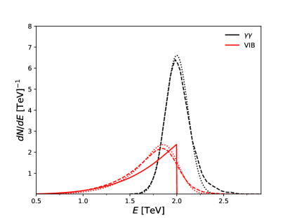
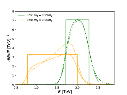
Figure 2: The figures show characteristic DM signal spectra, $dN_{\gamma}/dE_{\gamma}$, of the type discussed in Section 3, featuring sharp endpoints at or around $E_{0}=2$ TeV. Solid lines correspond to the physical, injected spectra, while dashed lines show the observed signal spectra as modeled by including the IRF of CTAO (see section 5.2). For comparison, dotted lines show the result of the physical spectrum convoluted with a Gaussian of width equaling the energy resolution displayed in Fig. 1. Left panel: Monochromatic line (black), Eq. (3.3), and VIB (red), Eq. (3.4). The solid, monochromatic line at $E_{\gamma}=m_{\chi}=2$ TeV is not shown explicitly. Right panel: The signal spectrum for two different box scenarios, Eq. (3.5); green (orange) curves show the case of the box width $\Delta E$ being smaller (larger) than the energy window. The DM mass for the narrow (wide) box shape in these examples is $m_{\chi}=4\ (2.87$) TeV. We note that the different areas under these curves directly reflect the different number of photons per annihilation, namely $N_{\gamma}=2$ for the line spectrum, $N_{\gamma}=1$ for VIB and $N_{\gamma}=4$ for box-shaped spectra.

In Fig. 2 we provide concrete examples to illustrate these spectral shapes. As apparent from the above list, furthermore, the exact shape of the spectra we consider here strongly depends on the details of the underlying particle model (in contrast to the spectra considered in Ref. [7]). This implies that the detection of such a signal would not only provide smoking gun evidence for particle DM, but immediately allow to reach far-reaching conclusions about the more general theory these DM particles are embedded in [5].

Eventually we will be interested in deriving CTA sensitivities in terms of projected upper limits on the (velocity-weighted) DM annihilation cross section $\langle\sigma v\rangle_{\mathrm{ann}}$, for a given spectral shape $dN_{\gamma}/dE_{\gamma}$. Let us therefore close this section by briefly reflecting about the expected size of $\langle\sigma v\rangle_{\mathrm{ann}}$ for thermally produced DM. In particular, the total annihilation rate required to produce the observed DM relic abundance in the early universe is often referred to as the ‘thermal’ annihilation rate, and numerically given by about $\langle\sigma v\rangle_{\rm therm}~{}\sim 2.1\times 10^{-26}~{}\rm{cm^{3}s^{-1}}$ for DM particles with $m_{\chi}\sim 1$ TeV [76]. For line signals, it is in principle possible that $\chi\bar{\chi}\to X\gamma$ is the dominant annihilation channel – e.g. because DM only couples to heavier, charged states [77] – in which case the correct ‘benchmark’ cross section is indeed $\langle\sigma v\rangle_{\rm therm}$. More generically, however, this channel will be suppressed by a loop-factor of $(\alpha_{\rm em}/4\pi)^{2}$ with respect to the tree-level annihilations that are responsible for setting the relic density, resulting in $\langle\sigma v\rangle_{\mathrm{ann}}\sim 10^{-31}~{}\rm{cm^{3}s^{-1}}$ and lower; however, near-resonant annihilation can lead to line signals significantly larger than this estimate [62, 64, 50] and non-perturbative effects can even result in present-day annihilation cross sections higher than the ‘thermal’ value responsible for setting the relic density in the early universe (prominent examples being Wino and Higgsino DM [49]). VIB signals, on the other hand, are inevitably accompanied by tree-level processes (without the additional photon in the final state) that set the relic density and hence generically suppressed only by a factor of $\sim{\alpha_{\rm em}}/\pi$ with respect to the ‘thermal’ rate. For box signals, finally, the relic density is often set by the same process that gives rise to the signal, namely $\chi\bar{\chi}\to\phi\phi$; in fact, the value of the relevant ‘thermal’ cross section can easily be a factor of a few higher because, for such an annihilation scenario, freeze-out would typically happen in a secluded dark sector (see Ref. [78] for how to determine the relic density in such cases).

4 Target Regions

In Section 3 we discussed spectral signatures of annihilating DM, related to the particle physics aspects of DM. In this section we turn our attention to the expected spatial distribution of cold DM, largely independent of its particle properties, and how this motivates our choice of target regions. Generally speaking, as evident from Eq. (3.1), close-by regions with a high DM density are good targets for observing DM annihilation signals. The GC region has the largest $J$-factor, Eq. (3.2), among all possible targets, making it arguably the best DM target from the point of view of the overall expected signal strength (even when taking into account that the uncertainty on the $J$-factor, $\Delta J$, is considerable). However, the GC hosts a rich environment of astrophysical gamma-ray emitters, resulting in complex backgrounds for DM searches.

Complementary targets to the GC are dwarf spheroidal galaxies, which have practically no astrophysical background in gamma rays [79], but are farther away and less massive, resulting in lower $J$-factors. Many dSphs are very faint in terms of visible gravitational field tracers (stars and gas), thus leading to substantial uncertainties in the DM density distribution, and hence $J$, also for these targets.

Below we discuss in more detail the GC target in Section 4.1, including astrophysical backgrounds, as well as dSphs in Section 4.2.

4.1 Galactic centre

Observational program.

There is a large number of independent science drivers that motivates an observational strategy for CTAO specifically targeting the GC region [29]. We follow the recommendation for the GC survey from that work and consider $9$ pointings centred at $l:\{\pm 1^{\circ},0^{\circ}\}$, $b:\{\pm 1^{\circ},0^{\circ}\}$, each with an observation time of $58.3$ hours. Effectively, this gives a total of $500$ hours of observation time of the GC with a roughly homogeneous exposure over the inner $4^{\circ}$ (see also Ref. [7] for further details, including full exposure maps).

We will base our analysis on this GC survey setup, but will optimize our region of interest (RoI) to comprise a region that is generally significantly smaller than the above mentioned $4^{\circ}$ (by maximizing the expected signal-to-noise ratio, see Section 5.1 for further details). Based on this observational (and analysis) strategy we simulate all signals and backgrounds using ctools v$1.6.3$ [80], a public software package developed for the scientific analysis of gamma-ray data.

Dark Matter Distribution.

Numerical $N$-body simulations of collision-less cold DM clustering, neglecting the effect of baryons, have over the past decades consistently found that DM halos develop a universal density profile on all clustering scales [81]. While there are differences in the exact parametrization of such a profile, its salient feature is that it is ‘cuspy’, i.e. it follows a power law $\rho_{\chi}\propto r^{-n}$ with $n\gtrsim 1$, at small (kpc) galactocentric distances $r$. Due to the limited resolution of $N$-body simulations, as well as the fact that baryonic feedback is expected to become more relevant close to the halo centres, it is however unclear whether the extrapolation of such power laws remains valid to sub-kpc scales.

From the purely observational side, stellar data and gas tracers of the gravitational potential are typically used to constrain the underlying DM density profile on Galactic scales (with gravitational lensing providing a competitive alternative on larger scales). While this method works well for large galactocentric distances, where DM dominates, the gravitational potential in the inner $\sim$kpc of the GC is dominated by baryons. DM density measurements therefore remain inconclusive at small scales, being consistent with both cuspy and more shallow inner density profiles. The latter are, in fact, also found in $N$-body simulations including baryons, indicating that cores of constant DM density can develop due to baryonic feedback on the gravitational potential [82]. For example, a high concentration of baryons typically leads to a more vibrant star formation rate and hence an enhanced supernova (SN) feedback due to the injection of significant amounts of energy on short timescales, effectively ‘heating’ DM and dispersing the cusp. DM halos with active super-massive black holes can show a similar effect. These processes are however not yet understood in sufficient detail. In fact, the presence of baryons could also have the opposite effect, since the cooling of baryonic gas in the GC region may well lead to an adiabatic contraction and hence a steepening of the DM density profile with respect to the one found in DM-only simulations [83].

For these reasons, we follow Ref. [7] (see also there for a more detailed discussion) and adopt two bracketing DM density profiles in the main part of our analysis: Einasto [84] as a representative of cuspy profiles and cored Einasto [82] to estimate a possible conservative lower bound for the expected limits on (and discovery potential of) a DM signal:

$$\rho_{\mbox{\tiny{\rm{Einasto}}}}(r)\hskip 5.69046pt=\hskip 5.69046pt\rho_{s}\hskip 2.84526pt\mbox{e}^{-\bigl{(}\frac{2}{\alpha}\bigr{)}\bigl{[}\bigl{(}\frac{r}{r_{s}}\bigr{)}^{\alpha}-1\bigr{]}}$$ (4.1)

$$\rho_{\mbox{\tiny{\rm cored\ Einasto}}}\!\left(r\right)=\begin{cases}\rho_{\mbox{\tiny{\rm Einasto}}}\!\left(r_{c}\right)&\textrm{if}\;r\leq r_{c}\\ \rho_{\mbox{\tiny{\rm Einasto}}}\!\left(r\vphantom{r_{c}}\right)&\textrm{if}\;r>r_{c}\end{cases}\,.$$ (4.2)

Here $\rho_{s}$ is the characteristic density, normalized to an average DM density of $\rho(r_{\rm{\odot}})=0.4$ GeV$/$cm³ at the same galactocentric distance as the sun ($r_{\odot}=8.5\ \mathrm{kpc}$), $r_{s}=20$ kpc is the characteristic radius and $\alpha=0.17$ is the Einasto shape parameter. The core radius is chosen as $r_{c}=1~{}\rm{kpc}$, which for this analysis essentially implies $\rho=const$ for the cored Einasto profile as we only focus on the inner few degrees of the GC. Tab. 1 lists the resulting J-factor values for the inner $2^{\circ}$ of the GC, as computed with DarkSUSY v$6$ [85] and cross-checked with CLUMPY v$3.0.1$ [86]. Here, we include for completeness also the often quoted Navarro-Frenk-White profile [87], which is similarly cuspy to the Einasto profile, for the same choice of parameters as adopted in Ref. [7]. For a more detailed discussion of how the choice of DM profile affects our results, we refer to Section 7.1.

	Angular Size [sr]	J-factor [$\rm{GeV^{2}cm^{-5}}$]
		Einasto	cored Einasto	NFW
$J_{0.5^{\circ}}$	$2.39\times 10^{-4}$	$3.48\times 10^{21}$	$1.93\times 10^{20}$	$2.65\times 10^{21}$
$J_{1^{\circ}}$	$7.18\times 10^{-4}$	$5.14\times 10^{21}$	$5.55\times 10^{20}$	$2.69\times 10^{21}$
$J_{1.5^{\circ}}$	$1.20\times 10^{-3}$	$5.53\times 10^{21}$	$9.38\times 10^{20}$	$2.67\times 10^{21}$
$J_{2^{\circ}}$	$1.67\times 10^{-3}$	$5.41\times 10^{21}$	$1.29\times 10^{21}$	$2.56\times 10^{21}$
$J_{2.5^{\circ}}$	$2.15\times 10^{-3}$	$5.27\times 10^{21}$	$1.64\times 10^{21}$	$2.49\times 10^{21}$
$J_{3^{\circ}}$	$2.63\times 10^{-3}$	$5.10\times 10^{21}$	$1.99\times 10^{21}$	$2.44\times 10^{21}$
$\sum J_{\leq 2^{\circ}}$	$3.83\times 10^{-3}$	$1.96\times 10^{22}$	$2.97\times 10^{21}$	$1.06\times 10^{22}$

Table 1: J-factors $[\rm{GeV}^{2}\rm{cm}^{-5}]$ for the benchmark DM profiles adopted in our GC analysis, as computed with DarkSUSY. $J_{\theta}$ indicates the J-factor for a concentric ring with outer radius $\theta$ and inner radius $\theta-0.5^{\circ}$, with a total angular size as indicated in the 2nd column. The last row states the total $J$-factor from the inner 2 degrees.

Background Components.

The fact that CTAO effectively uses the atmosphere as a calorimeter implies an inevitable source of background from misidentified CRs, independent of the target that is observed (in this sense, this could be called an ‘instrumental’ background). CRs hitting the upper atmosphere consist mainly of protons and electrons, with fluxes that are (at $\sim 100$ GeV) a factor of $10^{4}$ and $10^{2}$ times higher, respectively, than the diffuse gamma-ray flux [88, 89]. Though energy-dependent, the proton rejection rate is typically better than $10^{-2}$ due to the different shape of proton-induced showers compared to those induced by gamma rays. Electrons, on the other hand, produce almost identical shower shapes and are thus practically indistinguishable from gamma rays. The misidentified CR background has to be estimated based on detailed MC simulations of the shower evolution and the response of the instrument. As detailed in Sec. 5.1, we will use ctools v$1.6.3$ for the generation of mock data, automatically including this component.

In terms of astrophysical emission, the GC region is an active environment, rich with non-thermal emitters such as radio filaments [90], young massive stellar clusters [91], a number of pulsars, SNR shells etc., in addition to the super massive black hole, Sagittarius A* [92]. Furthermore, the whole region is embedded in the bright emission stemming from the Galactic CR population, producing gamma rays by interacting with magnetic fields, interstellar light and gas. This so-called Interstellar Emission (IE) extends to high latitudes at GeV energies [93], while at TeV energies it was so far only detected in the limited region of the GC Ridge [94]. In order to model this component we take advantage of a recent study [95] based on available GeV to PeV gamma-ray data (from Fermi LAT, Tibet AS$\gamma$, LHAASO and ARGO-YBJ), together with local charged cosmic ray measurements (from AMS-02, DAMPE, CALET, ATIC-2, CREAM-III and NUCLEON). Modelling the IE over such a wide energy range is achieved via two complementary approaches to describe the diffusion of CRs: in the so-called ‘Base’ models the diffusion coefficient is assumed to be constant throughout the Galaxy, while in the ‘Gamma’ models it is allowed to vary radially. Both sets of models are further divided in MIN and MAX setups in order to reflect uncertainties of the CR proton and helium source spectra, see Ref. [95] for more details. We choose Base MAX as our benchmark model, noting that current Gamma models were not tested in the vicinity of the GC, where by construction they should become increasingly brighter (and, likely, overshooting what can realistically be expected in this region). On the other hand, the Base models might somewhat underestimate the emission in the innermost region of the GC Ridge [96]. We explore these uncertainties in Sec. 8, but note that due to the methodology of the line search, background modelling is expected to have a rather limited impact on our results (as opposed to the case of continuum DM signals, cf. Ref. [7]).

In addition to the IE, our RoI also includes localised sources such as the point source associated with Sgr A*, HESS J1745-290[97], G0.9+01 and the recently discovered, still unidentified faint source HESS J1741-302[98]. We take into account these sources in our simulations, as well as the two extended sources HESS J1741-303 and HESS J1741-308. Although highly uncertain at small latitudes, finally, we further include a template of the Fermi bubbles (FBs) based on a recent analysis from Ref. [99].

When implementing the contribution from both point sources and FBs, we thus follow again the same modelling treatment as in Ref. [7]. For a more detailed discussion of all background components we therefore also refer to that reference.

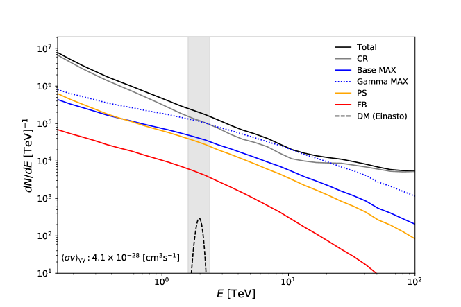
Figure 3: The total expected photon count (black solid line) from the individual background components, for the inner $2^{\circ}$ of the considered GC observation of 500 hr, that are included in the background simulations: Fermi Bubbles (FB, red), combined point sources (PS, orange), misidentified cosmic rays (CR, gray) and the diffuse gamma-ray emission (IE, blue). The solid line shows the benchmark model, Base MAX, included in the total count, while the dotted line indicates the alternative Gamma MAX model; see text for further details. For comparison, we also show a DM line signal (black dashed), assuming a DM mass $m_{\chi}=2\ \mathrm{TeV}$ and an annihilation strength that would result in a $5\sigma$ discovery; the shaded region corresponds to the size of the energy window used in the analysis in that case. Simulations are performed with ctools v$1.6.3$.

We display the expected count spectrum from the inner $2^{\circ}$ of the GC region, broken down into individual components, in Fig. 3. While the expected counts are clearly dominated by misidentified cosmic rays, the figure also illustrates that the astrophysical components discussed above can by no means be neglected for the analysis. For comparison, we also include a DM line signal (black dashed line), for a DM particle with mass $m_{\chi}=2$ TeV and annihilation cross section $\langle\sigma v\rangle_{\mathrm{ann}}=8.10\times 10^{-28}\ \mathrm{cm^{3}s^{-1}}$ which would lead to a $5\sigma$ discovery (see Sec. 5.3). The shaded region corresponds to the size of the ‘sliding’ energy window used to analyse such signals. We will discuss this analysis technique in detail in Sec. 5, but note already here that the total expected background count spectrum can be well described by a simple power law within the shaded region. As we will demonstrate, this observation makes it possible to robustly distinguish a sharply peaked DM signal, even if it is highly subdominant.

4.2 Dwarf Spheroidal Galaxies

The dSph satellites surrounding the Milky Way are old and DM-dominated systems. Due to their age and the lack of gas content, they are not expected to source any significant non-thermal emission. Consequently they are considered to be essentially background-free targets for DM signal searches [79], such that the detection of a gamma-ray signal might in itself constitute a smoking gun for the presence of particle DM (see e.g. Refs. [101, 102]). It is not only the substantial DM content (e.g. [103]) and their relative proximity that makes dSphs promising targets, but also the fact that they are distributed over a significant range of Galactic latitudes, including regions with low diffuse foreground emission. As of today, no gamma-ray signal has been conclusively associated with dSphs, either individually or as a population, and the corresponding upper limits have been used to set competitive constraints on the DM annihilation strength (summarised by e.g. Ref. [104]).

The statement that no dSph galaxy has been found to significantly emit gamma rays in the GeV or TeV band has recently been challenged by Crocker et al. [105], who report evidence of extended gamma-ray emission from the Sagittarius dSph (Sgr II). This emission appears as a well-known substructure inside the rather uniform FBs, which also has been coined the Fermi Bubbles’ cocoon region [106]. A possible explanation for such a signal from Sgr II would be a population of around 700 millisecond pulsars (MSPs), based on a strong correlation between the distribution of old stars in the system and the measured gamma rays. Indeed, the expected number of MSPs in dSphs only depends on the initial gas content (unlike in the case of the much higher stellar densities in globular clusters, where not only direct formation of binaries [107, 108, 109] but also formation in later stages via stellar encounters [110, 111, 112] plays a role). Based on this observation, a classical dSph like Fornax may host up to 300 MSPs [79]; since Sgr II contains about four times as many stars [113], $\mathcal{O}(1000)$ MSPs appear fully possible. On the other hand, the significance of Sagittarius’ gamma-ray emission reported in Ref. [105] could also be the result of mis-modelling the diffuse Galactic gamma-ray foregrounds [114] and hence remains the subject of a still ongoing debate. Let us in any case stress that a continuous background with a normalization as found in Ref. [105] will not affect in any appreciable way searches for monochromatic features. We tested this explicitly, conservatively allowing also for correspondingly re-scaled contributions from other dSphs, and found that our results (presented in Sec. 6.2) are affected only at the sub-percent level.

In an accompanying paper [115] we defined the most promising dSphs targets based on an updated analysis of stellar kinematic data and CTA observational strategy. While Ref. [115] is concerned about continuum spectra from DM annihilation and decay, our discussion of line searches here represents an extension of that work and follows the target selection and observational strategy considered there. Concretely, it is argued that the optimal strategy for CTA, given the relatively limited FoV, is not to observe as many targets as possible, but rather to focus on a limited number of dSphs with the highest chance of detection. The recommendation is to observe one classical and two ultra-faint dwarfs per hemisphere, namely Coma Berenices, Draco I and Willman 1 in the Northern hemisphere, as well as Reticulum II, the Sgr dSph and Sculptor in the South. In Tab. 2 we show the corresponding $J$-factors derived in Ref. [115], cf. Eq. (3.2), thereby updating the results from Ref. [116]. It should be noted that the observational strategy of CTA on one or more dSphs is not yet fully decided, but it was proposed [47] to dedicate 100 hr per target per year and per CTAO site, for a total of about 500-600 hr for both sites. Ref. [115] explores different strategies to optimally use an assumed total observing time of 600 hr. Here we will focus on the ‘conservative’ strategy, in terms of mitigating the impact of underestimated uncertainties of $J$-factor calculations, based on the observation of each of the six proposed candidates shown in Tab. 2 for 100 hr.

$\log_{10}J(0.5^{\circ})$ [$\rm{GeV}^{2}\rm{cm}^{-5}$]
dSph	CBe	DraI	Wil1	RetII	Scl	SgrII
CTA Group [115]	$19.5^{+0.9}_{-0.7}$	$18.7^{+0.3}_{-0.1}$	$19.1^{+0.6}_{-0.5}$	$18.9^{+0.9}_{-0.6}$	$18.4^{+0.1}_{-0.1}$	$18.9^{+1.8}_{-0.9}$
Bonnivar et al. [116]	$19.6^{+0.8}_{-0.8}$	$19.5^{+0.4}_{-0.2}$	$19.5^{+1.2}_{-0.6}$	$19.6^{+1.7}_{-0.7}$	$18.5^{+0.1}_{-0.1}$	$-$

Table 2: $J$-factors with mean standard deviations for a selection of dSph galaxies, as defined in Eq. (3.2), averaged over an RoI with radius $0.5^{\circ}$. Following Ref. [115], we include in our analysis the dSphs Coma Berenices (CBe), Draco I (DraI), Willman I (Wil1), Reticulum II (RetII), Sculptor (Scl) and the Sgr dSph (SgrII). For comparison, we also show the corresponding $J$-factors from an older compilation [116].

Traditionally, dSphs were only considered in the context of generic DM annihilation or decay spectra, not in the context of searches for pronounced spectral signatures (see, however, Ref. [22] for an exception). The latter searches, see also below in Sec. 5 for a detailed description, are by construction less limited by the presence of astrophysical backgrounds. This implies that it is in general favourable to focus on the region with the highest $J$-factor, namely the GC. However, given that CTA is anyway expected to dedicate substantial observation time to dSphs, we will also perform a sensitivity study for these targets here, based on the observational strategy discussed above. As it turns out, the CTA spectral line sensitivities from dSphs might in fact (almost) become comparable to those from the GC, in case the DM density profile in the Milky Way is cored rather than cuspy (i.e. a GC $J$-factor that is unfavourably small, combined with optimistic assumptions about the largest $J$-factors in dSphs).

5 Analysis

In the past, different strategies have been followed to search for DM signals with sharp spectral features. The most recent such analysis of the H.E.S.S. collaboration [117], e.g., adopted a fully data-driven approach based on two spatially distinct ‘ON’ and ‘OFF’ regions, respectively. Here, both regions are modelled as containing the same astrophysical and instrumental background; the ‘OFF’ region is assumed to contain no further emission components, such that any potential excess in the ‘ON’ region can be attributed to a DM signal. For current gamma-ray telescopes, this approach has proven highly successful also in searches for exotic signals with a broader energy distribution [118]. Given the increased DM sensitivity of CTA, the bright large-scale interstellar emission in the GC region can no longer be ignored [119, 7]. This would make this specific ON/OFF technique more challenging to use.

An alternative avenue is to model the astrophysical background components explicitly. The sliding energy window technique – as e.g. adopted by the Fermi-LAT collaboration [120, 121, 21], but also in earlier IACT studies [122, 123, 124, 22] – aims to implement this approach in an as data-driven and model-independent way as feasible. Realizing that the specific types of signals we are interested in here vary much faster with energy than any of the expected background components, the basic analysis idea is to divide the total energy domain into overlapping narrow energy windows, each window covering only a few times the instrumental energy resolution. This allows remaining agnostic about the nature of the background, and to model the cumulative (instrumental and astrophysical) background as a simple parametric function with parameters fit directly to the counts inside this narrow energy range. For our default analysis we follow this approach, modelling the total counts locally as a power law in energy.

A somewhat more sophisticated method of the background estimation is to separate the astrophysical and instrumental background components, noting that information about the latter is already contained in the IRFs. Indeed, these IRFs are based on a CR spectrum at the top of the atmosphere that is not, unlike the gamma-ray component, partially unknown but in fact well measured up to at least 100 TeV [125, 126, 127] (with percent-level precision up to 1 TeV [128]). This would motivate to use an interpolation of the misidentified CRs as provided by the IRF; only the intrinsic astrophysical background would then be locally modelled as a power law, convoluted with the IRF. As a result, the overall background description and sensitivity to DM improves over the simple fit directly on the counts, as described above; on the other hand, this approach is more dependent on explicit assumptions about the instrument performance (which will be more accurately known once the instrument is fully operational). Following this alternative approach can thus be used as an indication of how much potential gain in sensitivity one may eventually hope for, compared to the more conservative pre-construction sensitivity derived with our default analysis procedure.

In the following, we describe our benchmark analysis procedure in terms of the generation of mock data for the chosen RoI (Sec. 5.1), explain in more detail how we model background and signal components inside the sliding energy window (Sec. 5.2) and lay out the general analysis pipeline to derive exclusion limits and discovery sensitivities (Sec. 5.3). Later, in Sec. 7, we will explicitly discuss how modifying the assumptions underlying the benchmark analysis settings defined here would impact our results (presented in Sec. 6).

5.1 Data generation and analysis regions

Based on the observational strategies and expected signal and astrophysical background components outlined in Sec. 4, we generate mock data using ctools v$1.6.3$. The exact definition of the analysis RoIs, and the masking that we adopt, depends on the target region:

 

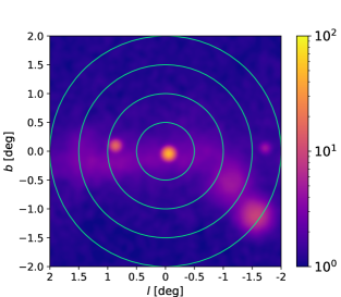
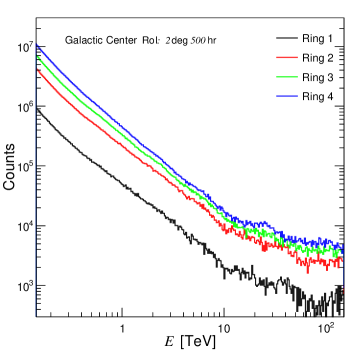
Figure 4: Left. Visualisation of the spatial binning geometry over a skymap of the GC background simulation described in Sec. 4.1. In Galactic coordinates, the figure shows the region $(b,l)=(-2^{\circ}..2^{\circ},-2^{\circ}..2^{\circ})$. The color scheme represent the counts in the energy range $[1.55,2.51]$ TeV with a pixel of size $(0.05^{\circ})^{2}$ and a Gaussian smoothing with the same size. Right. Integrated background photon count for each spatial bin, for a specific MC realization, where Ring$\ 1$ refers to the innermost and Ring$\ 4$ to the outermost region. The sum of the four histograms shown here can thus directly be compared to the (on average) expected photon count displayed as black line in Fig. 3. The histogram has a log-even binning of $100$ bins per decade, similar to the width used in our analysis.

Galactic Centre.

The GC survey will result in an almost isotropic exposure of the inner few degrees of the GC. We restrict our analysis to the inner $2^{\circ}$ of this survey, as motivated below, and divide this RoI into four spatial bins consisting of concentric rings of width $0.5^{\circ}$ (Tab. 1 lists the corresponding angular sizes and J-factor values). Fig. 4 shows a skymap of the whole RoI illustrating this spatial binning configuration (left panel) and a realisation of the total photon count – including misidentified CRs, point sources, the default (base-max) interstellar emission model (IEM) and Fermi bubbles – for each of the spatial bins (right panel). In the left panel, the three point sources HESS J1745-290 (centre), G0.9+01 (centre left) and HESS J1741-302 (right) are clearly distinguishable by eye, as well as the IE (concentrated along the Galactic plane). The photon count in the outer parts of the RoI (Ring 4), on the other hand, is dominated by misidentified CRs. Features in the spectrum between about $5$ and $10$ TeV reflect different spectral cuts in the transition region between the MSTs and SSTs; still, as visible in the right panel of the figure, a power law locally provides a reasonable description of the spectra across the entire energy range. It also becomes clear that up to energies of a few TeV, the photon count is so large that one would expect DM limits to be affected by the accuracy to which CTAO’s energy resolution and effective area are known; beyond multi-TeV energies, on the other hand, the limiting factor will be Poisson noise. We will return to this observation in Sec. 7.4.

Dividing the RoI in the GC region into several spatial bins is a relatively common procedure and motivated by the different morphologies of signal and background components, see, e.g., Refs. [130, 12, 131]. In Sec. 7.2 and Appendix A.2 we will discuss alternatives to our default analysis setting illustrated in Fig. 4, and show that the final DM limits and discovery prospects are rather robust with respect to the exact choice of the RoI and binning scheme. In particular, concentric ring binning gives the highest statistical power to discriminate a DM signal among the binning geometries that we checked explicitly, while providing an equivalent $\chi^{2}$ score of the background fit.

Dwarf Spheroidal galaxies.

We model the DM content of dSph galaxies ($J$-factor and its uncertainties, assuming a log-normal distribution) as stated in Tab. 2, based on the recent work developed within CTA [115]. We also follow the suggested observational strategy, i.e. we assume 100 hr for each of the targets shown in the table. Note that here we use $J$-factors calculated within 0.5 degrees of the centre of each dSph, in order to optimize the expected DM signal. Further increasing the size of the disk would not significantly enhance the sensitivity, see also Appendix A.2 for a related discussion about how to choose the RoI in the context of the GC. For the purpose of constructing the likelihood, see further down, we choose only one spatial bin per dSph; this is a simplification given the angular resolution of CTAO [47], but justified for our analysis which emphasizes spectral shapes over morphology. Given that all selected dSphs are located at high latitudes, finally, we neglect any potential IEM emission and model only the (misidentified) CR backgrounds.

5.2 Component modelling inside sliding energy window

As explained above, the mock data are generated based on a realistic implementation, as of current knowledge, of all relevant astrophysical (and signal) components in the respective RoIs. For the analysis of the data, on the other hand, we adopt a much simpler, parametric description of all components related to the ‘background’ (i.e. everything but the DM signal with its characteristic spectral shape). In particular, we will explore two strategies:

1. Power law on counts. As our benchmark analysis strategy, we aim to remain fully agnostic about the ‘background’ processes, other than assuming that they lead to a spectrum much less localized in energy than the DM signal. We therefore model the sum of the total counts (astrophysical and instrumental) as a power law,

   $$\mu^{\mathrm{bg}}_{ij}=b_{j}\int_{\Delta E_{i}}dE\,E^{-\gamma_{j}}\,,$$ (5.1)

   Here, $j$ denotes spatial bins and $i$ energy bins, and $b_{j}$ and $\gamma_{j}$ describe normalization and spectral index of the power law, respectively. With this ansatz, any assumption about the instrument performance is removed from the analysis step (but of course not from the generation of mock data).

2. Power law on gamma-ray flux. As an alternative analysis strategy we estimate the misidentified CR component in the total counts directly from the IRF, using ctools’ ctmodel, as given by the grey line in Fig. 3. We note that, once the instrument is fully operational, an alternative to determine this component would be an auxiliary measurement from an empty area on the sky. For the astrophysical background component, on the other hand, we assume that a simple power law locally provides a satisfactory description of the gamma-ray flux. We then estimate the contribution to the observed counts by convoluting this ansatz with the effective area shown in Fig. 1. The combined background model for the counts, including CRs and astrophysical gamma rays, is thus

   $$\mu^{\mathrm{bg}}_{ij}=N_{ij}^{\rm CR}+b_{j}\int_{\Delta E_{i}}dE\,A_{\rm{eff}}(E)E^{-\gamma_{j}}\,,$$ (5.2)

   where $N_{ij}^{\rm CR}$ is the expected number of counts due to unidentified cosmic rays; $b_{j}$ and $\gamma_{j}$ describe normalization and spectral index, respectively, of only the gamma-ray component. Here, the effective area in this simplified form, neglecting the PSF and energy dispersion, is introduced exclusively to improve the (numerical) performance of the analysis. We checked explicitly that this description reproduces the results from a full ctools implementation (with a source spectrum following a power law) to sufficient accuracy.

In Appendix A.4, cf. Fig. 19, we will get back to the question of how well these two background descriptions fit the actual (mock) data.

As far as the DM component is concerned, we are interested in the detailed shape of the signal and simply convolving the intrinsic annihilation spectrum $dN_{\gamma}/dE_{\gamma}$ with the effective area is no longer sufficient. Instead, we fully model the instrument response using ctools. For a line, VIB and box signal, cf. Eqs. (3.3, 3.4, 3.5), this results in the count spectra shown in Fig. 2. We thus model the signal component as

$$\mu^{\chi}_{ij}=\nu_{j}\int_{\Delta E_{i}}dE\,\zeta(E),$$ (5.3)

where $\nu$ is the signal normalization and $\zeta$ the photon count of the signal spectrum convolved with the IRF (as displayed in Fig. 2). The normalization of $\nu_{j}$ is fixed by Eq. (3.1). In practice, we use this equation to calculate the total signal count rate only once, leading to some value of $\nu_{0}$ for the whole RoI (or, for the case of dSphs, the sum of all targets) and a reference cross section $\langle\sigma v\rangle_{\mathrm{ann}},_{0}$ and DM mass $m_{0,\chi}$. For a fixed value of the DM mass, $m_{\chi}$, $\nu_{j}$ is then directly related to the annihilation rate that is to be constrained as $\nu_{j}/\nu_{0}=(m_{0,\chi}/m_{\chi})^{2}(\langle\sigma v\rangle_{\mathrm{ann}}/\langle\sigma v\rangle_{\mathrm{ann}},_{0})(J_{j}/J_{\rm tot})$, where $J_{j}$ ($J_{\rm tot}$) is the $J$-factor associated to the spatial bin $j$ (the total RoI).

The final task is to optimize the analysis region – the sliding energy window – such that it is small enough for the effective description of the background model to hold, but at the same time large enough to give sufficient statistical power to test the DM signal. The benchmark setting that we adopt in our analysis is a sliding energy window of width $\Delta=8\sigma_{\mathrm{res}}(E_{0})$, centred on the putative DM signal localized at $E_{0}$ (for a wide box, with width $\Delta E>\Delta$, we choose the energy window instead to be centred on the upper edge of the box spectrum, cf. the right panel of Fig. 2). Here, $\sigma_{\mathrm{res}}$ is the energy resolution of CTAO, as depicted in Fig. 1. As detailed in Appendix A.1, this choice of $\Delta$ is motivated by increasing the window size until the signal significance begins to converge while at the same time ensuring that the background model (described above) still gives a good fit to the data. We use an energy binning of three energy bins per $\sigma_{\mathrm{res}}$, i.e. we are in some sense effectively working in the limit of an unbinned analysis (in energy). Given the instrumental count normalization, our setup guarantees more than 10 photons per bin even at the highest energies considered in the analysis.

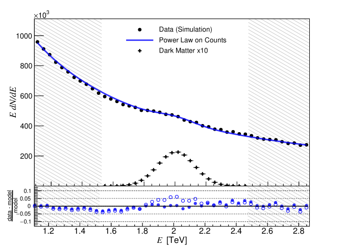
Figure 5: Illustration of the sliding energy window technique to identify signals with sharp spectral features. Mock data points (black dots) are based on the full background model, for the GC survey, and a monochromatic signal component at $E_{0}=2$ TeV with a normalization that would allow a $5\sigma$ discovery. The white area that is not hatched corresponds to the sliding energy window, of width $8\times\sigma_{\mathrm{res}}(E_{0})$, within which the analysis is performed. Black crosses show the expected signal component (multiplied by a factor of 10 for better visualization). The blue solid line is the result of fitting the data with a monochromatic signal component on top of a simple power law. The lower panel shows residuals with (solid circles) and without (empty circles) including the signal component in the fit.

In Fig. 5 we illustrate the analysis procedure by showing an explicit example of a monochromatic DM line injected into the data, which is then fitted by the assumed signal component and a simple power law on the ‘background counts’. The region between the shaded areas is the sliding energy window inside which the analysis is performed. We indicate the true signal with black crosses, scaled by a factor of 10 for better visibility, and the best-fit model (power law plus signal) with a solid blue line. The residual plot in the lower panel gives a good visual impression of how well the power law fits the background inside the analysis region – even though it does not necessarily do so for a larger energy range. In what follows we detail how this observation can be used to derive (expected) sensitivity limits for such line signals.

5.3 Statistical procedure

Within each sliding energy window we implement a binned likelihood based on Poisson statistics, $P\left[\left.{n}_{ij}\right|{\mu}_{ij}\right]=\prod_{i,j}e^{-\mu_{ij}}{\mu_{ij}^{n_{ij}}}/{\left(n_{ij}\right)!}$, where $\bm{\mu}=\{\mu_{ij}\}$ denotes the model prediction and $\bm{n}=\{n_{ij}\}$ the (mock) data counts. The energy bins (indicated by an index $i$) are taken to be much smaller than the instrument’s resolution, thus effectively implementing an unbinned approach; the spatial bins, indicated by an index $j$, refer to the RoIs defined in Fig. 4 (for the GC analysis) or the individual galaxies stated in Tab. 2 (for the stacked dSph analysis), respectively. The model prediction depends on the signal normalization $\nu$, and various background model and other nuisance parameters which we collectively denote as $\bm{\theta}$.

Treatment of systematic uncertainties.

Clearly, instrumental systematic uncertainties are challenging to model for a telescope still under construction. Even if the underlying event counts are uncorrelated, as assumed here, the finite energy resolution of CTA will correlate noise deriving from systematic deviations between the true and assumed IRFs. Here we take a parametric approach to estimate such systematic noise by introducing additional nuisance parameters $\eta_{i}$, one for each energy bin $i$, to rescale counts expected from the model prediction as $\mu_{i}\rightarrow\eta_{i}\mu_{i}$. We model the covariance of these nuisance parameters by assuming multivariate normal distributions with means $\langle\eta_{i}\rangle=1$ and a covariance matrix $\Sigma$ with variance $\sigma$. The off-diagonal part of the covariance matrix is thus modelled as

$$\Sigma_{ii^{\prime}}=\sigma^{2}\exp{\left[-\frac{(E_{i}-E_{i^{\prime}})^{2}}{2(\lambda\,\Delta E)^{2}}\right]}\,,$$ (5.4)

where $\lambda$ denotes the correlation length and $\Delta E\equiv\sigma_{\mathrm{eres}}(E_{0})$, with $E_{0}$ being the energy at the center of the analysis window. We find that this functional form describes the results of dedicated MC simulations very well when adopting a characteristic length scale $\lambda\simeq 1.5$, see Appendix A.4 for further details. For the variance we choose $\sigma=0.025$ which, at face value, is significantly larger than the $\sim$1% design goal of CTAO [29]. This choice avoids artificially strong limits due to an overfitting of the specific numerical IRF (and/or IEM) model realization that is used in our analysis. See also Sec. 7.4 for a discussion of how the treatment of systematic uncertainties impacts our final results.

Construction of likelihoods.

Following the description above, the total likelihood that we adopt for the GC analysis is given by

$$\mathcal{L}(\nu,\bm{\theta})\hskip 5.69046pt\propto\hskip 5.69046pt\prod_{i}\prod_{j}P[n_{ij}|\eta_{ij}\mu_{ij}]\,\exp\left[{-(1-\eta_{ij})\Sigma_{ii^{\prime}}^{-1}(1-\eta_{i^{\prime}j})}\right]\,,$$ (5.5)

where the indices $i$ ($j$) run over all energy (spatial) bins within the sliding energy window, and a summation over the energy bins $i^{\prime}$ in the covariance part is implicit. We recall that our model description is given by $\mu_{ij}=\mu^{\chi}_{ij}(\nu)+\mu^{\mathrm{bg}}_{ij}(\bm{\theta}_{\rm bg})$, with $\nu$ being the signal normalization and $\bm{\theta}_{\rm bg}=\{b_{j},\gamma_{j}\}$ describing the background normalizations and slopes of every spatial bin that is considered (per energy window); the full list of nuisance parameters for the GC likelihood is thus given by $\bm{\theta}=\bm{\theta}_{\rm bg}\cup\{\eta_{i}\}$.

The likelihood for dSphs is constructed by multiplying (stacking) the individual likelihoods for each separate dSph observation, taking into account their respective $J$-factors and associated uncertainties. For each dSph galaxy we model the likelihood for the true $J$-factor to follow a log-normal distribution $\mathrm{Log}\mathcal{N}$ around the mean observed value (following, e.g., Ref. [132]), $\bar{J}_{j}$, with the standard deviation $\sigma_{J,j}$ of $\ln J$ fitted to the mean absolute deviation stated in Tab. 2. Since the DM flux is directly proportional to the $J$-factor, we thus arrive at the total likelihood (see also Ref. [133, 102, 134])

$$\mathcal{L}(\nu,\bm{\theta})\hskip 5.69046pt \propto \prod_{j}^{\rm dSph}\mathrm{Log}\mathcal{N}\left[\log_{10}(J_{j})|\log_{10}(\bar{J}_{j}),\sigma_{J,j}\right]$$

$$\times\prod_{i}P[n_{ij}|\eta_{ij}\mu_{ij}]\,\exp\left[{-(1-\eta_{ij})\Sigma_{ii^{\prime}}^{-1}(1-\eta_{i^{\prime}j})}\right]\,.$$

Denoting with $\nu$ the signal normalization that would correspond to a putative target with $J_{\rm eff}\equiv\sum_{j}\bar{J}_{j}$, the model description is now given as $\mu_{ij}=\mu^{\chi}_{ij}(\alpha_{j}\nu)+\mu^{\mathrm{bg}}_{ij}(\bm{\theta}_{\rm bg})$, with $\alpha_{j}\equiv J_{j}/J_{\rm eff}$, and the complete list of nuisance parameters is $\bm{\theta}=\{\log_{10}(J_{j}),\eta_{i},b_{j},\gamma_{j}\}$.

Expected limits and discovery prospects.

Exclusion limits must correctly account for statistical downward fluctuations in the photon count, for a given signal strength, while discovery limits should avoid falsely rejecting the background-only hypothesis in the presence of upward fluctuations of the background. In order to distinguish the hypotheses of signal plus background and background only, respectively, we estimate both types of limits by implementing a standard likelihood ratio test [135], based on the test statistic (TS)

$${\rm TS}(\nu)\equiv-2\log{\frac{\mathcal{L}(\nu,\hat{\hat{\bm{\theta}}})}{\mathcal{L}(\hat{\nu},{\bm{\hat{\theta}}})}}\,.$$ (5.7)

Here, $\hat{\hat{\bm{\theta}}}$ is the conditional estimate (best fit) for $\bm{\theta}$ under the hypothesis $\nu\geq 0$. The best-fit estimates for the signal normalization and nuisance parameters are given by $\hat{\nu}$ and $\hat{\bm{\theta}}$, respectively. We use the Migrad algorithm [136, 137] in ROOT’s MINUIT package to maximize (profile over) the likelihoods given in Eqs. (5.5, 5.3) to obtain these quantities.

In order to produce sensitivity curves for expected exclusion limits, one must generate mock data without a signal component. Taking into account that the signal normalization is non-negative, one-sided $95\%$ upper exclusion limits (U.L.) are found by increasing the signal normalisation, $\nu$, until

$${\rm TS}_{\mathrm{U.L.}}(\nu)=2.71\,.$$ (5.8)

In order to derive the sensitivity for discovery, on the other hand, one has to generate mock data including a signal with some normalization $\nu^{\prime}$. A $5\,\sigma$ discovery, corresponding to a p-value of $5.74\times 10^{-7}$, can be claimed when the test statistics for the background only hypothesis ($\nu=0$) on this data set evaluates to

$${\rm TS}_{\mathrm{discovery}}\equiv TS(0)=23.75\,.$$ (5.9)

In practice, this involves gradually increasing $\nu^{\prime}$ until the best-fit signal normalization $\hat{\nu}$ satisfies the above condition. We note that, for the energies and analysis window considered here, a signal discovery will always correspond to significantly more than 10 signal photons.

Since the likelihood is a function of the (mock) data, limits derived from Eqs. (5.8, 5.9) will necessarily be subject to statistical fluctuations. Rather than creating a large number of mock datasets to derive the median limits, and their variances, we will here adopt the Asimov dataset method [138]. This method allows to extract both results from a single, fiducial dataset that is defined by the observed photon counts in each bin being exactly equal to their expectation values. For further details on the construction of the Asimov dataset, including explicit validation checks with MC simulations, see Appendix A.3.

6 Results

	Galactic Centre	dSphs
Exposure time	500 hr	100 hr per target
DM density profile	Einasto [7.1]	$J$-factors in Tab. 2
RoI and binning	$4$ rings of width $0.5^{\circ}$deg [A.2]	Single RoI per dSphs, $0.5^{\circ}$
Mask	none [7.2]	none
IEM	Base MAX [7.3]	none
Analysis method	Sliding energy window, PL assumption on counts
Window size	$8\sigma_{\mathrm{res}}(E_{0})$ [A.1]
Systematic uncertainty	$2.5\%$, per energy bin [7.4]

Table 3: Summary of benchmark settings and assumptions for the analysis performed in this work. All our main results, presented in Sec. 6, are exclusively based on these settings. Numbers in parentheses link to the subsections where we assess the impact of varying the respective assumption or analysis setting on our results.

All results in this section will assume our set of benchmark assumptions, summarised in Tab. 3. In particular, in Sec. 6.1 we present the sensitivity for exclusion and discovery of DM self-annihilating to a pair of monochromatic gamma rays from the GC, and in Sec. 6.2 the sensitivity resulting from a stacked analysis of six dSphs. Finally, in Sec. 6.3, we provide results for the case of other sharp spectral features that can originate from DM annihilation, focussing on box-shaped and VIB-like signals.

6.1 Galactic Centre

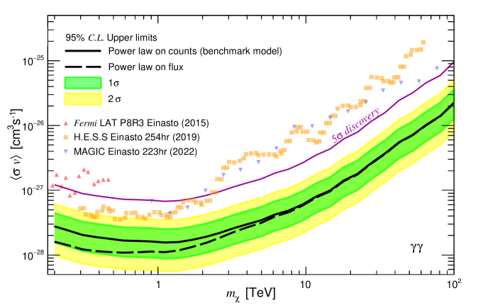
Figure 6: Median of expected $95\%~{}C.L.$ upper limits on the annihilation of DM into a pair of gamma-ray photons (black) as well as the $5\sigma$ discovery potential (purple), as a function of the DM mass $m_{\chi}$. The green and yellow bands show the expected variance of the median upper limits, as indicated, and data points summarize $95\%~{}C.L.$ limits previously obtained by Fermi LAT [139], H.E.S.S. [117] and MAGIC [24]. (Note that a significant scatter between mass bins is expected for a limit on actual data, as opposed to the median of limits derived from many MC realizations; the treatment of systematic uncertainties, furthermore, partially differs from the analysis adopted in this work). The limits projected for CTA are based on the assumption of an Einasto DM profile and $500$ hours of observation of the inner GC, adopting our benchmark modelling of the background component in the analysis (solid lines); for comparison, we also indicate (with dashed black lines) the mean upper limits resulting from the more aggressive analysis method that relies on modelling the astrophysical gamma-ray flux – rather than the total counts – as a power law.

In Fig. 6, we show the expected median $95\%~{}C.L.$ upper limits (black) and the $5\sigma$ discovery potential (purple) of the DM line signature. While solid lines are the result of our default analysis strategy (power-law background on the measured counts), dashed lines show the alternative approach, where the power-law assumption is made on the gamma-ray fluxes instead. As stressed in Sec. 5.2, the default approach neglects our knowledge of the IRFs and therefore results in more conservative estimates of the sensitivity. The inner (green) and outer (yellow) bands show the 1 $\sigma$ and 2 $\sigma$ confidence level of our sensitivity estimate, respectively, as derived from the Asimov dataset (for further discussion, see Appendix. A.3). The lower DM mass threshold in this figure is set to 200 GeV, from the requirement of the lower edge of the sliding energy window to not fall below 100 GeV. We prefer to not use the lowest bins at this stage because the effective area of CTAO drops rapidly when going below 100 GeV, cf. Fig. 1, causing the current IRF estimate to be more uncertain.

As demonstrated in the figure, the projected CTA sensitivity to spectral line signatures improves upon current limits by ground-based experiments (notably HESS [117]) by a factor of $\sim$2 at 1 TeV, and by up to one order of magnitude in the multi-TeV range. Such an improvement is in rough agreement with what one may expect from an increase of exposure alone, as a consequence of doubling the observation time and a larger effective area (cf. right panel of Fig. 1). Below about 300 GeV, the CTA sensitivity is expected to become worse than limits reported by the Fermi LAT [139]. It is also intriguing to compare the current bounds to the CTA discovery potential. The fact that CTA would potentially allow the robust discovery of a line signal above around 3 TeV, without being in tension with any known limits, offers exciting prospects for detecting heavy DM candidates. For example, this corresponds to the upper mass range of thermally produced Wino-like DM [140, 141]. Let us stress that the results obtained in Fig. 6 were obtained with the initially targeted ‘Alpha’ configuration of the instrument; we find that a fiducial ‘Omega’ configuration corresponding to a later construction stage would result in a further improvement of the reported limits by about a factor of two.

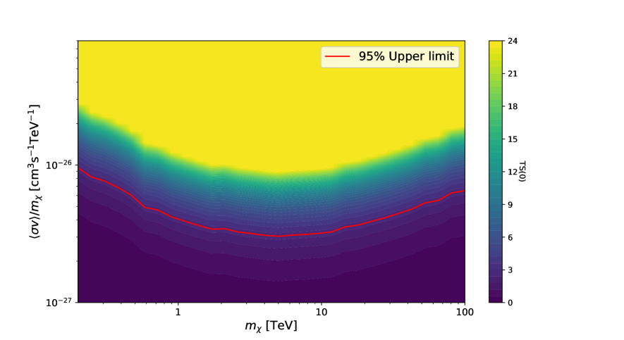
Figure 7: Contour plot of the local test statistic for a monochromatic line signal from DM annihilations $\chi\chi\to\gamma\gamma$, as a function of $\langle\sigma v\rangle/m_{\chi}$ and the dark matter mass $m_{\chi}$. To guide the eye, we apply a cap of TS $=23.75$ in this figure, corresponding to a 5 $\sigma$ discovery. The $95\%$ C.L. limit, corresponding to the black solid line in Fig. 6, is indicated with a red line for comparison. The full likelihood tables for both limits and discover potential are available for download at zenodo [142].

Consequently, CTAO data will likely also have a decisive impact on global fits of theories beyond the standard model that contain multi-TeV DM candidates (see, e.g., Refs. [143, 144, 145]). To facilitate such parameter scans we provide in Fig. 7 the full binned TS, from which the likelihood, up to an overall normalization, follows from Eq. (5.7). Note that, for plotting reasons, we choose here $\langle\sigma v\rangle/m_{\chi}$ rather than $\langle\sigma v\rangle$ for the $y$-axis. This figure complements the limits at a given confidence level shown in Fig. 6, and illustrates how quickly it becomes impossible to reject the signal hypothesis once the intrinsic signal strength reaches a certain value (while at low signal strengths the test statistic, and hence the likelihood, remains rather flat). We provide a tabulated version of the likelihood at zenodo [142].

6.2 Dwarf Spheroidal Galaxies

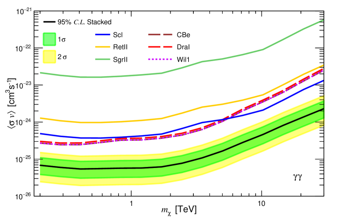
Figure 8: CTA sensitivity limits of a dark matter line signal from $\chi\chi\to\gamma\gamma$, assuming $100$ hour observations of the individual (colored) and stacked (black) dSphs. The green and yellow bands show the expected variance of the stacked limits at the 1 $\sigma$ and 2 $\sigma$ level, respectively. For the individual objects, as indicated in the legend, solid lines styles are used for objects targeted by the southern array, while other lines styles are used for objects targeted by the northern array.

We extend the DM line search to a combined analysis of the most promising dSphs for DM indirect detection, as described in Section 4.2. The result for the median expected limits on such a signal is shown as a solid black line in Fig. 8, along with the expected variance of these limits at the 1 $\sigma$ and 2 $\sigma$ level (green and yellow bands, respectively). As expected, the sensitivity resulting from the observation of dSphs is significantly worse, by more than two orders of magnitude, than the sensitivity shown in Fig. 6 for the GC case. On the other hand, the DM distribution close to the GC is much more uncertain than the $J$-factor determination of dSphs. This may reduce the GC sensitivity by a factor of 10 with respect to the default assumption of an Einasto density profile, see the discussion in Section 7.1 below, which could in fact make line limits obtained through dSph observations (marginally) competitive. Concerning discovery, the above discussion also makes clear that identifying a line(-like) signal in at least one dSph would be an extremely strong case in favour of a DM interpretation if – and in fact only if – an identical spectral shape is seen from the direction of the GC.

Let us stress that the sensitivities shown in Fig. 8 crucially depend not only on the mean value and standard deviations of the $J$-factors, as stated in Tab. 2, but in principle on their entire probability distribution. When eventually inferring limits from actual data taken by CTAO, it is thus important to include the full likelihoods from state-of-the-art kinematical analyses rather than just derived values for mean and standard deviation of the $J$-factors. Incorrectly modelling the $J$-factor distribution beyond their first two moments may, in fact, easily affect overall DM limits by a factor of a few.

In Fig. 8 we also present, for comparison, the $95\%$ exclusion limits for the individual targets. In principle, these limits could be roughly scaled with the square root of the observation time in order to estimate the effect of implementing different observational strategies. From the figure one can see that sensitivities derived from individual observations of Coma Berenices, Draco and Willman 1 are comparable, and that the combined (stacked) limits improve the best individual limit by about a factor of three. Indeed, these results might suggest that for the specific case of line searches a better observational strategy could be to focus the entire 600 hr of available observation time on the three dSphs visible with the Northern array (for a general and more detailed discussion of optimizing dSph observations for DM searches, we refer to Ref. [115]).

6.3 General Signal Shapes

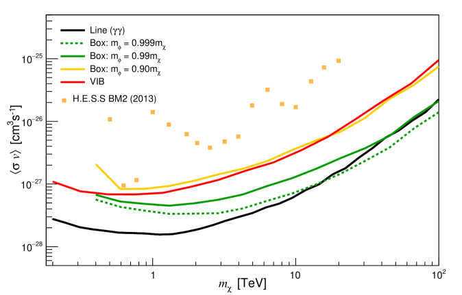
Figure 9: Expected median $95\%~{}C.L.$ exclusion limits, from GC observations, for the spectral shapes shown in Fig. 2: VIB (red), a relatively wide box with $m_{\phi}=0.9\,m_{\chi}$ (orange) and a narrow box with $m_{\phi}=0.99\,m_{\chi}$ (green). For comparison, we also show the case of an extremely narrow box with $m_{\phi}=0.999\,m_{\chi}$ (dotted green) and the result for a monochromatic line signal (black, same as in Fig. 6). Note that the analysis windows for the narrow box spectra are centred around $E=m_{\chi}/2$, the wide box spectrum is centred at the upper edge $E=(m_{\chi}+\Delta E)/2$, while those for VIB and line spectra are centred around $E=m_{\chi}$; as a consequence, the lowest mass points that we include in our analysis are given by $m_{\chi}=0.4$ TeV and $m_{\chi}=0.2$ TeV, respectively. We also indicate previous $95\%~{}C.L.$ limits obtained by H.E.S.S. [146] for a signal shape model (BM2 from Ref. [17]) that closely resembles the VIB signal studied here, rescaled to the DM profile adopted in this analysis for the sake of comparison (see footnote 10 for further details).

We next assess the impact of deviations from an exactly monochromatic signal shape. As discussed in Sec. 3, such deviations can appear quite commonly, and are in fact intricately linked to the specific particle nature of the annihilating DM particles. For definiteness, we consider here the same examples of such signal shapes as the ones introduced in Fig. 2, and show in Fig. 9 the corresponding sensitivity of CTA for our benchmark set of assumptions for GC observations.

The sensitivity to a VIB-like spectrum (red line) is very roughly a factor of $\sim 5$ worse than that to a monochromatic signal (black line), consistent with previous findings [123, 146]. The reason for this is a combination of three effects: i) the VIB signal is intrinsically weaker by a factor of 2 because there is only one photon produced per DM annihilation, as opposed to two photons in the case of annihilation to $\gamma\gamma$, ii) the peak of the VIB signal occurs at slightly smaller energies than for a monochromatic signal, cf. the left panel of Fig. 2, where the (soft) background contribution is larger, and iii) the VIB signal is less sharp than a line signal and hence not quite as easily distinguishable from the (power-law) background. On the other hand, DM annihilation to a photon pair is necessarily loop-suppressed, at order $\mathcal{O}(\alpha_{\rm em}^{2})$, while the emission of a single photon happens at $\mathcal{O}(\alpha_{\rm em})$. Depending on the DM model, the sensitivity of CTA to the VIB signature may thus still result in significantly more constraining limits than the sensitivity to a line signal.

Turning to the case of box-like signal shapes, there is an additional complication in that the intrinsic signal is not centred at $E=m_{\chi}$, as for VIB and $\gamma\gamma$, but at smaller energies (down to $E=m_{\chi}/2$ for narrow boxes). The sensitivity to a box signal at $m_{\chi}=1$ TeV, for example, should thus be compared to the sensitivity for a line signal at $m_{\chi}=500$ GeV – but only after multiplying the former by a factor of 4 because the signal strength is explicitly proportional to $m_{\chi}^{-2}$, cf. Eq. (3.1). On the other hand, there are four photons that are produced per annihilation, compared to two for the case of the $\gamma\gamma$ line. In summary, the sensitivity curve to an extremely narrow box – which closely resembles a monochromatic line – should in principle coincide exactly with the sensitivity curve for $\gamma\gamma$ after it has been shifted by a factor of 2 both downwards (towards smaller $\langle\sigma v\rangle$) and to the left (towards smaller $m_{\chi}$). For illustration we show in Fig. 9 the case of a very narrow box with $m_{\phi}=0.999\,m_{\chi}$ (green dotted line) which, indeed, follows this expectation to a very good accuracy. Compared to the ‘monochromatic box limit’ represented by the dotted green line, the sensitivity generally worsens as the box widens. This can be clearly seen for the explicit examples of a narrow box ($m_{\phi}=0.99\,m_{\chi}$, green line) and a wide box ($m_{\phi}=0.9\,m_{\chi}$, orange line) shown in the figure. For a narrow box, the origin of this sensitivity loss is simply that the signal becomes more and more smeared out, cf. point iii) above. For a wide box – where the analysis window is centred on the upper end of the signal rather than on $m_{\chi}/2$, cf. the right panel of Fig. 2 – an additional loss of sensitivity results from the fact that the low-energy part of the signal is completely dominated by the background (and hence not even included in the analysis window anymore).

In analogy to the concluding comment that we made about the sensitivity to a VIB-like signal, it is worth stressing that box-like signals are produced at leading order in perturbation theory, i.e. without any generic suppression in $\alpha_{\rm em}$. This implies that CTA will be able to provide highly competitive limits on the class of DM models that produce such a signal shape. One way of illustrating this claim is to compare the sensitivity shown in Fig. 9 to the benchmark ‘thermal’ annihilation cross section of $\langle\sigma v\rangle\sim 2\cdot 10^{-26}\,{\rm cm}^{3}/{\rm s}$ that is needed to produce DM in the early universe, in the simplest models of thermal freeze-out (see, e.g., Ref. [78] for a recent discussion and precision determination of this quantity). We can thus conclude that CTA can actually have a significantly better sensitivity to TeV DM that is thermally produced by annihilations of the type $\chi\chi\to\phi\phi$ than for models where DM directly annihilates to standard model particles (a case studied in detail in Ref. [7]). For $\gamma\gamma$ and VIB signals, on the other hand, such a direct comparison is not as easily possible since these signals are intrinsically suppressed by powers of $\alpha_{\rm em}$.

For comparison, we further include in the figure previous VIB limits obtained by H.E.S.S. [146]. We are not aware of corresponding published limits for box-like spectra (but see Ref. [28] for an earlier CTA sensitivity estimate). Let us finally briefly comment on a significant theoretical activity in modelling the exact shape of the spectral endpoint feature for $\chi\chi\to\gamma\gamma$ annihilations, after taking into account radiative corrections [53, 54, 55, 56, 57, 58, 59, 60, 61]. Since these corrections are necessarily model-dependent, at least to some extent, a detailed discussion is clearly beyond the scope of this work. However, let us remark that the deviations from a monochomatic line are typically significantly less pronounced than the case of the narrow box shown with a green solid line in Fig. 2. To a very good accuracy, one can therefore obtain limits on such ‘generalized line signals’ by simply convolving a given spectrum with the CTAO energy resolution, i.e. a Gaussian of width $\sigma_{\rm res}$, and then rescaling our limits for $\gamma\gamma$ by the ratio of the resulting peak height to that for a monochromatic line, $2\times(2\pi\sigma_{\rm res}^{2})^{-1/2}$. We expect the uncertainty associated with this method to be less than the difference between the solid and dotted green lines in Fig. 9 – and thus significantly less than the statistical uncertainty in the limit prediction itself.

7 Discussion

In this section we explore the robustness of the results presented in Sec. 6, by studying how the individual benchmark assumptions that we made, cf. Tab. 3, impact our final DM limits. We focus here on our main target, the Galactic Centre, and the most decisive aspects with respect to sensitivity projections for this target, namely the assumed DM density distribution (7.1), the RoI masking (7.2), the interstellar emission modelling (7.3), and systematic uncertainty choices (7.4). In the Appendix, we further complement this by exploring the impact of the analysis window size (A.1) as well as the RoI size and shape (A.2).

7.1 Dark matter profiles

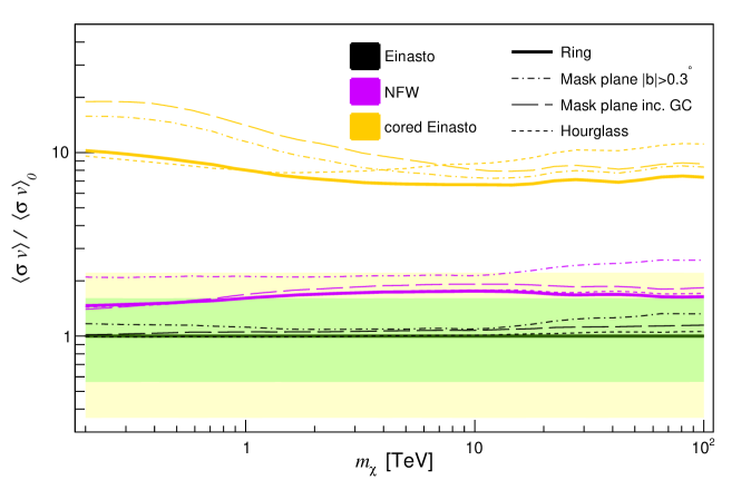
Figure 10: Impact of varying the DM profile (solid lines) and masking (other line styles) of the GC RoI on the CTA DM sensitivity, expressed as $95\%~{}C.L.$ exclusion limits normalized to the benchmark result (displayed as black solid line both in Fig. 6 and here). The light green and yellow bands show the $1\sigma$ and $2\sigma$ variance of the expected limit for these benchmark settings (summarized in Tab. 3). All black lines refer to an Einasto profile, while magenta and orange lines show the situations for an NFW and a cored Einasto profile, respectively, with profile parameters as defined in Sec. 4.1. Non-solid line styles correspond as indicated to different ways of masking the RoI, illustrated in Fig. 11.

As described in Sec. 4.1, the DM density profile is poorly constrained observationally in the inner region of our galaxy, in particular within the inner $\sim 0.7$ kpc relevant for the RoI of our analysis. Motivated by high-performance N-body simulations, we chose the commonly used Einasto profile as a benchmark assumption for the density profile. In Fig. 10 we quantify how the sensitivity of CTA to a monochromatic DM signal worsens in case the DM distribution follows instead the NFW profile (solid magenta line) or an Einasto profile with a core size of 1 kpc (solid orange line). We find that the sensitivity is affected by less than a factor of 2 in the case of the NFW profile, well within the statistical spread of the expected $95\%\,C.L.$ limit that CTA will achieve. For a cored profile, on the other hand, our sensitivity prediction would worsen by up to one order of magnitude. This loss of sensitivity is by far dominated by a corresponding decrease in the total $J$-factor, cf. Tab. 1, as is expected for an analysis comparing components with very different spectral shapes. Unlike in the case of a continuum signal [7], in other words, the fact that the largely isotropic DM signal becomes morphologically degenerate with the bright CR background is much less important.

Incidentally, this observation also implies that it is straight-forward to translate the projected limits shown in Fig. 6, to a very reasonable accuracy, to the case of DM decaying via $\chi\to\gamma\gamma$. In this case one just has to replace $\frac{1}{2}\left\langle\sigma v\right\rangle(\rho_{\chi}/m_{\chi})^{2}\to\Gamma\rho_{\chi}$ in Eq. (3.1), where $\Gamma$ is the decay rate for this channel. A limit of $\left\langle\sigma v\right\rangle<\left\langle\sigma v\right\rangle_{\rm max}$, therefore, is equivalent to a minimal lifetime of $\tau_{\chi\to\gamma\gamma}>2m_{\chi}\left\langle\sigma v\right\rangle_{\rm max}^{-1}D/J$, where the ‘$D$-factor’ $D\equiv\int_{\Delta\Omega}d\Omega\int\!\!d\ell\,\rho_{\chi}$ for decaying DM is defined in analogy to the $J$-factor for annihilating DM. Note that this lifetime constraint applies to a DM particle with mass $2\,m_{\chi}$, i.e. twice the original mass.

7.2 Region of interest

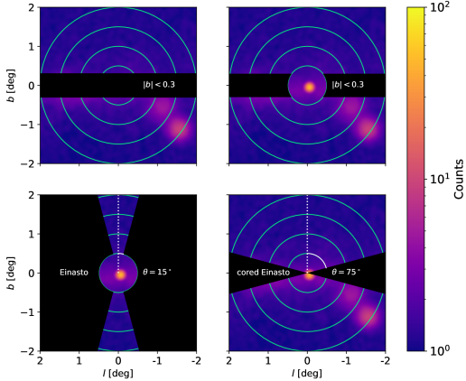
Figure 11: Illustration of various masks of the RoI that we tested in our analysis. In Galactic coordinates, each of the four panels shows the region $(b,l)=(-2^{\circ}..2^{\circ},-2^{\circ}..2^{\circ})$. The color scheme reflects the counts in the energy range $[1.55,2.51]$ TeV per pixel of size $0.01^{\circ}\times 0.01^{\circ}$ with a Gaussian smoothing of $0.05^{\circ}$. Top left: Masking the Galactic plane. Top right: Masking the Galactic plane while including the inner central region. Bottom left: Hourglas shape, with opening angle S/N-optimized for an Einasto (or NFW) profile. Bottom right: Hourglas shape, with opening angle S/N-optimized for a cored profile.

While our benchmark analysis strategy includes the full RoI, a disc of radius $2^{\circ}$ centred on the GC, it is reasonable to ask wether increasing the RoI or masking regions with low signal-to-noise ratio (S/R), i.e. bright backgrounds, could improve the sensitivity. As we discuss in more detail in Appendix A.2, increasing the RoI beyond $2^{\circ}$ would in fact hardly improve the sensitivity, but potentially lead to larger systematic uncertainties related to the background modelling. The more general question of optimizing the shape of the analysis region was studied in detail before, e.g. Refs. [147, 18], typically resulting in the conclusion that analysis regions with hourglass-like shapes tend to provide maximal S/N. In the bottom panel of Fig. 11 we show two such hourglass shapes for illustration, characterised by a parameter $\theta$ that describes the opening angle of the analysis region. In the bottom left panel, the value of $\theta=15^{\circ}$ is motivated by typical results from optimizing S/N for a cuspy profile (NFW or Einasto), though we note in this case S/N does in fact not very strongly depend on $\theta$; in the bottom right panel, $\theta=75^{\circ}$ is a more typical value that optimizes S/N for a cored profile. We indicate the impact of such a masking on our benchmark sensitivities with dotted lines in Fig. 10.

An alternative to simply maximizing S/N is to chose a mask that aims at making one of our main analysis assumptions as realistic as possible, namely that the background emission can be approximated by a power law in a narrow energy range. As the Galactic plane is expected to contain a significant number of (subthreshold) sources that could affect the validity of this assumption, we thus consider a mask that fully covers the plane, $|b|<0.3^{\circ}$, as depicted in the top left panel of Fig. 11. The (very limited) impact of such a mask on the sensitivities is indicated with dash-dotted lines in Fig. 10. Finally, we also consider the option of masking the Galactic plane but including the GC in the analysis, cf. the top right panel of Fig. 11, and show the impact on the DM sensitivity with dashed lines in Fig. 10.

We observe that our sensitivities are largely robust to masking schemes, worsening by factors of at most two in extreme cases due to the loss in photon statistics (which, in turn, is directly proportional to a corresponding reduction of the effective $J$-factor). This implies that line limits eventually derived from real data will also be very robust, only mildly affected by even very aggressive cuts in the analysis region in order to minimize the impact of underlying modelling uncertainties.

7.3 Background model dependence

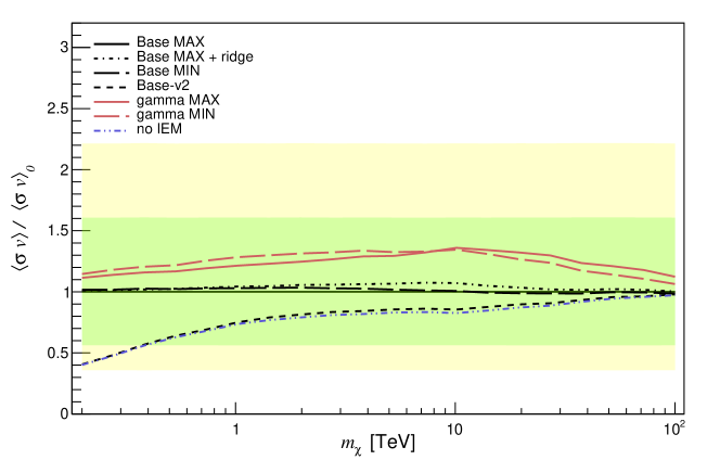
Figure 12: Impact of varying the IEM model on the CTA DM sensitivity, expressed as $95\%~{}C.L.$ exclusion limits normalized to the benchmark result (displayed as black solid line both in Fig. 6 and here). The different model setups are described in detail in Sec. 4.1, with line styles as indicated in the legend. The light green and yellow bands show the $1\sigma$ and $2\sigma$ variance of the expected limit for the benchmark settings (summarized in Tab. 3).

Modelling of the interstellar emission is highly uncertain in the Galactic plane, given presently available data, and even more so in the inner region of the Galactic Center. Thus, the question arises of how this affects the sensitivity predictions derived here. As discussed in Sec. 4.1 we choose the Base MAX model as our benchmark analysis setting. In Fig. 12 we explore how the predicted limits would change should a different model turn out to better describe the real data.

We observe that the difference with the Base MIN model is negligible, while in the case of gamma models the sensitivity could worsen by up to $50\%$. In the case of the conservative IEM used in Ref. [148], dubbed Base-v2, the sensitivities would instead improve by up to $50\%$, especially at low energies. Note that this exercise optimistically assumes a perfect model for the emission which, however, should not qualitatively affect our conclusions. In particular, the expected impact on the limits is of a similar order as the expected variation of the central limit prediction at the $1\sigma$ level, and hence not very significant.

The rather limited dependence of our results on the exact implementation of background modelling is, in fact, one of the expected features of our analysis method. As long as the background does not itself contain sharp spectral features, the identification of these types of DM signals will remain relatively robust. In particular, the limit (or signal) significance will to a large degree only be affected at the level of the noise contribution, i.e. the overall background normalization. This is in contrast to other template-based analyses; see, e.g., Ref. [7] for a discussion of how the background modelling impacts the search for a DM signal with a smooth spectrum.

7.4 Impact of instrumental systematics

A realistic analysis will always be affected by some level of systematic uncertainty. This could have an instrumental origin, e.g. related to event reconstruction or misclassification, or stem from modelling uncertainties. In this subsection we approach this issue in a general way and explore the impact of systematic uncertainty following the parametric approach introduced in Sec. 5.3.

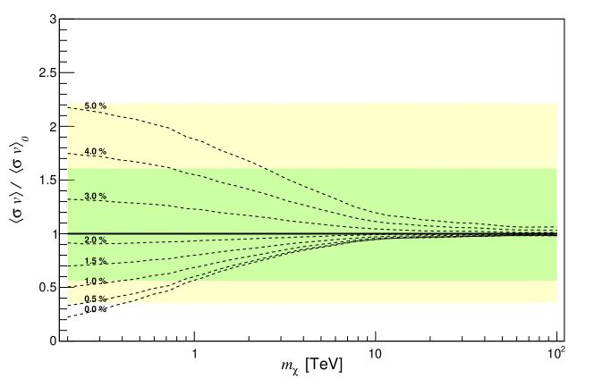
Figure 13: Impact of varying the level of systematic uncertainty, cf. Eq. (5.4), on the CTA sensitivity to a monochromatic DM signal, expressed as $95\%~{}C.L.$ exclusion limits normalized to the benchmark result (displayed as black solid line both in Fig. 6 and here). The light green and yellow bands show the $1\sigma$ and $2\sigma$ variance of the expected limit for the benchmark settings (summarized in Tab. 3).

In Fig. 13, we show the effect of varying the overall normalization of the covariance matrix, Eq. (5.4), which we refer to as ‘the systematic uncertainty’ $\sigma$. As expected, the figure demonstrates that systematic uncertainties only impact the limits at low energies, where the total photon count is large. Increasing the systematic uncertainty from our benchmark value of 2.5% to 5%, for example, worsens the limits by up to a factor of 2.2 (for a DM mass of $m_{\chi}=200$ GeV). Not taking into account the effect of systematic uncertainties at all, on the other hand, would result in limits that are too optimistic by up to a factor of 4. Let us briefly mention that Fig. 13 illustrates the effect of varying $\sigma$ for our benchmark analysis method of modelling the entire non-signal photon count as a power law; implementing instead the more aggressive modelling based on a power law of the fluxes, cf. Sec. 5.2, results in quantitatively almost identical results.

Our results are thus considerably less sensitive to instrumental uncertainties than what is familiar from generic DM spectra with a broader shape [7]. Again, the reason is that we chose an analysis method that is very efficient in singling out sharp spectral features from an otherwise feature-less ‘background’. Incidentally, this is also the explanation for why the sidebands in Fig. 6 have a constant width, almost independent of the DM mass (as even more clearly visible in Figs. 12 and 13); we checked that this starts to change when increasing the level of systematic uncertainty to unrealistically large values $\sigma\gg 5$%, leading to a broadening of the sidebands at small masses.

In summary, systematic uncertainties dominate the overall uncertainties of the projected limits up to DM masses of a few TeV, from where statistical uncertainties begin to be more important. Even for sub-TeV DM masses, however, a mis-modelling of instrumental effects is not expected to affect limits by more than a factor of $\sim$2 w.r.t. to our results presented in Fig. 6.

8 Conclusions

The Cherenkov Telescope Array Observatory has a great potential to probe thermally produced DM at TeV energies [7]. Due to its superior energy resolution compared to current gamma-ray facilities, furthermore, it is expected to be the most sensitive instrument to identify possible sharp features in gamma-ray spectra at these energies, like monochromatic ‘line’ signals. The detection of such features would provide smoking-gun evidence for the decay or annihilation of DM particles, and may in fact reveal decisive information about the underlying microphysical model that describes these particles.

In this article we have presented a detailed study to estimate the expected sensitivity of CTA to such distinct spectral features, using up-to-date observational strategies and the latest IRFs taking into account updated telescope configurations. In particular, our analysis is based on a 500 hr extensive Galactic Centre survey and 600 hrs of dSph galaxy observations. For the latter, we follow an accompanying CTA consortium paper [115] focusing on DM in dSphs and work under the assumption that these 600 hr of total observation time will be split evenly among six dSphs, three per hemisphere. We explore the commonly considered case of a monochromatic signal, originating for example from the loop-suppressed annihilations of a pair of DM particles into two photons, but also the possibility of more general spectral shapes that would constitute clear evidence for a DM signal. For the latter, we use two generic spectral templates that may originate from three-particle final states including a single photon (‘virtual internal bremsstrahlung’) and the annihilation of DM into subsequently decaying mediator particles (‘box’-like spectra), respectively.

In addition to using the latest information related to the CTAO instrument and observational plans, as well as a rather broad focus on spectral features beyond the commonly performed ‘line’ searches, this work improves upon previous CTA sensitivity projections in the following:

• We use state-of-the-art models of the astrophysical gamma-ray background in the GC that include updated interstellar emission models and three known point sources.

• We perform a range of optimization studies and carefully explore various types of systematic uncertainties. In particular, we investigate the impact of various DM density profiles, regions of interest and masking, and of background and instrumental systematics. For the latter, we explicitly add an overall $2.5\%$ systematic uncertainty, on top of taking into account correlations in the expected instrumental uncertainties.

• We assess two main variants of the commonly adopted sliding energy window analysis technique to identify sharp spectral features: i) locally modelling the total simulated count rate for the (instrumental and astrophysical) background as a simple power law, and ii) an alternative method in which the astrophysical and instrumental background components are separated, noting that information about the latter is already contained in the IRFs; in this case the power law is fit to the gamma-ray flux that is then convoluted with the IRFs and added to the simulated CR counts. The former method is more conservative and constitutes our default analysis procedure. The second approach improves DM sensitivity but depends on the IRF model – and serves to illustrate the potential gain in sensitivity that one may eventually hope for with real data and an exquisite understanding of the instrument in full operation mode.

Our main results are shown in Fig. 6. In particular, the CTA sensitivity to spectral line features is expected to improve upon current limits from ground-based experiments (notably H.E.S.S.) by a factor of $\sim 2$ at 1 TeV, and by up to one order of magnitude in the multi-TeV range, which to a large degree is an effect of increased exposure. At high energies, even a 5 $\sigma$ discovery of a signal is conceivable, for DM annihilation cross sections just below current limits. It should be stressed that a fiducial ‘Omega’ configuration of CTAO would allow a further improvement of the limits by a factor of $\sim$ 2. As discussed in Sec. 6.1, both constraining and discovery potential of CTA have profound implications for particle models of DM at the TeV scale, and we therefore also provide the full binned TS, cf. Fig. 7, to consistently include the CTA sensitivity to monochromatic DM signals in, e.g., global scans of the underlying parameter space of such models.

We generally find that prospects to detect line-like DM signals in dSphs are significantly suppressed w.r.t. what can be achieved with GC observations (Fig. 8). On the other hand, one should keep in mind that these targets are very robust as far as modelling of the astrophysical background is concerned. As discussed in Sec. 7.1, they may therefore still constitute relevant complementary targets to detect monochromatic or similarly sharp spectral features in case the concentration of the DM density close to the GC turns out to be very unfavourable. Projected limits on spectral features beyond the simplest possibility of a monochromatic line, cf. Fig. 9, also appear very promising. In particular, the sensitivity to VIB-signals will improve in accordance with what is expected for line signals; for scenarios where the dominant DM annihilation channel is into a pair of mediator particles, furthermore, CTA may even be able to test the thermal production of DM for masses up to around 50 TeV.

In summary, this study complements Ref. [7] on the CTA sensitivity to generic DM signals from the GC region in two important ways: by focussing on possible DM annihilation channels that stress the discovery rather than the constraining power of the instrument and, related, by adopting a very different analysis strategy that is specifically tailored to identify spectral (as opposed to spatial) features. The exciting combined message from these two works is that CTA is guaranteed to close significant parameter space of thermally produced DM and that, at the same time, a truly groundbreaking discovery remains in fact a fully viable possibility.

Appendix A Analysis details

A.1 The width of the sliding energy window

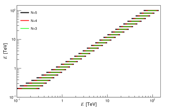
Figure 14: Energy window sizes $\Delta=2N\times\sigma_{\mathrm{res}}(E_{0})$ for $N=3,4,5$, where $\sigma_{\mathrm{res}}(E_{0})$ is the energy resolution shown in Fig. 1. The benchmark setting adopted in our analysis is given by $N=4$.

For the analysis presented in the main part of this article we adopted a sliding energy window with a width of $\Delta=8\sigma_{\mathrm{res}}(E_{0})$ around a signal centered at $E_{0}$, where $\sigma_{\mathrm{res}}(E_{0})$ is the energy resolution of CTAO at that energy (as depicted in Fig. 1). Fig. 14 illustrates this choice, along with the effect of increasing or decreasing $\Delta$ with respect to the energy resolution.

In this appendix we address the question of how to optimize the sliding energy window size for the purpose of our analysis, i.e. how to chose $N$ in

$$\Delta=2N\times\sigma_{\mathrm{res}}(E_{0})\,.$$ (A.1)

It is clear that the identification of a sharp spectral feature and a power-law background at lower and higher energies will fail if the analysis window is too small compared to the energy resolution, i.e. for $N\lesssim 1$. In fact, one should expect that the determination of the background power law will monotonically improve as $N$ is increased, and as a result the determination of the exact signal normalization should improve as well. In Fig. 15 we confirm this expectation by plotting the test statistics under the background-only hypothesis, but with a monochromatic DM signal present in the data; for illustration, we choose here a signal at $E_{0}=0.2$ TeV ($E_{0}=100$ TeV) in the left (right) panel. Naively, the fact that TS$(0)$ continuously rises with $N$ would then suggest that the optimal analysis approach is to formally take the $N\to\infty$ limit, i.e. to include the entire energy range observable by CTAO in the analysis.

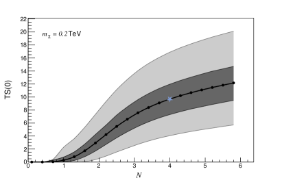
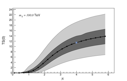
Figure 15: Effect of varying the sliding energy window size, cf. Fig. 14, on the test statistic under the background-only hypothesis, but with an (arbitrarily normalized) monochromatic DM signal present in the data. The left and right panel show the case of a monochromatic signal at $E_{0}=0.2$ TeV and $E_{0}=100$ TeV, respectively. The star at $N=4$ indicates the value adopted in our analysis. For $N\gtrsim 4$ the gradient becomes less steep, such that the increased statistical power in identifying the signal no longer outweighs the likewise increasing uncertainty connected to the underlying background modelling (see text for further discussion).

However, this would not only be computationally unreasonably expensive – due to a proliferation of nuisance parameters capturing systematic uncertainties – but is in fact at odds with the very idea of the sliding energy window technique, which is based on the assumption of a very simple (power-law) description of the background inside the analysis window. The point is that by increasing $N$ one will always formally increase the statistical power to determine the model parameters, while by decreasing $N$ the assumption of a power law will necessarily improve, thus removing systematic uncertainty and background-model dependence (mathematically speaking, in the limit $N\to 0$, the assumption of a power-law background becomes exact). Conversely, for an energy range that is too wide, the simplistic assumption of a power law will result in unsatisfactory background modelling.

Fortunately, inspection of Fig. 15 reveals a clear transition between two regimes, which we use as guiding principle for choosing the ‘optimal’ window size: for $N\lesssim 4$, the information gain from increasing $N$ is still substantial, while for $N\gtrsim 4$ the TS only increases rather modestly. Recalling that the statistical significance of the derived limit scales roughly as $\sqrt{TS(0)}$, increasing the sliding energy window further thus hardly affects the limits anymore. For $N\lesssim 4$, furthermore, a power law can still be expected to describe the actual background very well (see also Appendix A.3). We find a qualitatively very similar behaviour across the entire range of observable energies, and that the exact choice of $N\approx 4$ has only a minor impact. Let us note that similar criteria to determine the optimal window size have been adopted before, e.g. in Ref. [123] in terms of the relative change directly in the expected DM limit, rather than a change in TS$(0)$, when allowing for generic deviations of some fiducial background model from the power-law assumption used in the analysis.

A.2 Choosing the Galactic centre region of interest

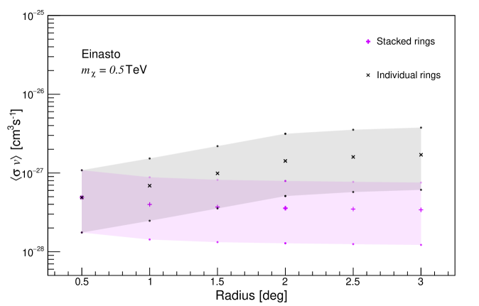
Figure 16: Median $95\%\,C.L.$ exclusion limits (black ‘$\times$’) and their $1\,\sigma$ variance (grey shading) on the DM annihilation cross section that result from RoIs consisting of individual rings centered on the GC, with width $0.5^{\circ}$ and outer edge at the stated radius. Purple ‘$+$’ symbols and shadings indicate the corresponding limits when instead combining all rings up to the stated radius. All limits are based on a DM mass of $m_{\chi}=0.5\mathrm{\ TeV}$ DM and an Einasto profile for the DM distribution.

For our analysis, as illustrated in Fig. 4, we consider a spherical RoI with radius $2^{\circ}$ centered on the GC. In this appendix we motivate this choice. For this purpose, we show in Fig. 16 how individual rings contribute to the constraining power of the analysis. As expected, the sensitivity monotonically increases (purple band) with the total size of the RoI – but it is also clear that it saturates relatively quickly. This is because the constraining power from the individual rings deteriorates when going to larger radii. Three effects are responsible for this behaviour: i) an increased background (or noise) photon count due to the larger area of outer rings, ii) a $J$-factor that slightly decreases beyond about $2^{\circ}$, see also Tab. 1, and iii) a decreased CTAO exposure further away from the GC, beyond about $2^{\circ}$, given the adopted observational strategy. On the other hand, similar to the discussion in Appendix A.1, it is desirable to keep the RoI small in order to minimize systematic uncertainties in our background modelling.

Fig. 16 is based on an Einasto profile and a DM mass of $m_{\chi}=0.5$ TeV, but we note that other profiles or DM masses result in a qualitatively very similar behaviour. In particular, increasing the size of the RoI beyond 2 degrees hardly impacts the sensitivity in any of the cases we have considered. In our analysis, we hence fix for simplicity the GC RoI to $2^{\circ}$ for all masses and over all energies (for the case of dSphs we choose $0.5^{\circ}$, following an analogous reasoning). We note that already a simple S/N analysis arrives at a similar conclusion, namely that for GC line searches it is favourable to focus on RoIs with a scale of the order of a few degrees [147].

Let us finally mention that a corresponding S/N optimization can also be performed for the masking, with S (N) denoted as $\mu^{\chi}$ ($\mu^{\chi}+\mu^{\rm bg}$) in Sec. 5.3, resulting in the hourglass shapes shown in Fig. 11. In this case, however, we find that the S/N ratio only has a rather weak dependence on the opening angle $\theta$, so the exact value of $\theta$ does not affect our analysis in any appreciable way.

A.3 Asimov Dataset vs. Monte Carlo realizations

In this Appendix we derive our analytic estimates of the median and the variance of the sensitivity limits, based on evaluating the Asimov data set, and verify these estimates by direct comparison to MC simulations. The defining property of the Asimov data set $A$ is that its best-fit parameter values coincide with the true model parameter values realized in nature (or taken as input values for MC simulations). This implies

$$\mathcal{L}_{A}(\hat{\nu},\hat{\bm{\theta}})=\mathcal{L}_{A}(\nu_{\rm true},\bm{\theta}_{\rm true})\,,$$ (A.2)

where $\nu_{\rm true}$ is the true signal strength and $\bm{\theta}_{\rm true}$ are the values of all nuisance parameters.

In Eq. (5.7) we introduced the standard log-likelihood test statistic $\text{TS}(\nu)$ as a function of the hypothesized signal strength $\nu$, for any given data set. Under the Wald approximation, TS takes the form of a parabola around the best-fit value. For a signal strength that is physically constrained to be non-negative (i.e. $\nu\geq 0$), the likelihood then takes the form of a truncated Gaussian, with [138]

$$\text{TS}(\nu)\simeq\tilde{q}_{\nu}\equiv\begin{cases}\frac{\nu^{2}}{\sigma_{A}^{2}}-\frac{2\hat{\nu}\nu}{\sigma_{A}^{2}}&\nu\geq\hat{\nu}\quad\&\quad\hat{\nu}<0\\ \frac{(\nu-\hat{\nu})^{2}}{\sigma_{A}^{2}}&\nu\geq\hat{\nu}\quad\&\quad\hat{\nu}\geq 0\\ 0&\nu<\hat{\nu}\end{cases}\,,$$ (A.3)

where the standard deviation $\sigma_{A}$ is to a very good accuracy independent of the best-fit value $\hat{\nu}$. In practice, we can most easily extract $\sigma_{A}$ by evaluating the above equation on an Asimov data set without signal, for which $\hat{\nu}=0$, resulting in $\sigma_{A}={\nu}\big{(}{{\tilde{q}_{\nu}}^{A,0}}\big{)}^{-1/2}$ for any given value of $\nu$. We further note that an alternative way of stating Eq. (A.3) is by formally solving for the assumed signal strength,

$$\nu=\begin{cases}\hat{\nu}+\sqrt{\hat{\nu}^{2}+\bar{\nu}^{2}}&\hat{\nu}<0\\ \hat{\nu}+\bar{\nu}&\hat{\nu}\geq 0\end{cases},$$ (A.4)

where we have introduced $\bar{\nu}\equiv\sqrt{\tilde{q}_{\nu}}\sigma_{A}$.

Let us now consider the case with no signal, i.e. $\nu_{\rm true}=0$. The best-fit value $\hat{\nu}$ in any given dataset is then still a random variable, distributed according to a normal distribution $f^{\hat{\nu}}=\mathcal{N}(0,\sigma_{A})$ with variance $\sigma_{A}$. The value of $\nu$ that produces a given value of $\tilde{q}_{\nu}$ (e.g. $\tilde{q}_{\nu}=2.71$ for a 95% upper limit) thus also becomes a random variable, with distribution

$$f_{\tilde{q}_{\nu}}^{\nu}=\frac{1}{\sqrt{2\pi}\sigma_{A}}\begin{cases}\frac{1}{2}[1+\frac{\bar{\nu}^{2}}{\nu^{2}}]\exp\left[{-\frac{(\frac{1}{2}\nu-\frac{\bar{\nu}^{2}}{2\nu}-\bar{\nu})^{2}}{2\sigma_{A}^{2}}}\right]&\hat{\nu}<0\\ \exp\left[{-\frac{(\nu-\bar{\nu})^{2}}{2\sigma_{A}^{2}}}\right]&\hat{\nu}\geq 0\end{cases}\,.$$ (A.5)

Note that the required signal strength to set an upper limit based on the best-fit value $\hat{\nu}$ thus has an asymmetric distribution, as a direct consequence of the constraint $\nu\geq 0$. For comparison, the distribution of upper limits for an unconstrained signal strength would simply be

$$f_{q_{\nu}}^{\nu}=\mathcal{N}(\bar{\nu},\sigma_{A})\,,$$ (A.6)

i.e. as in the second line of Eq. (A.5) but without the restriction to $\hat{\nu}\geq 0$.

An important implication of an asymmetric distribution is the appearance of asymmetric sidebands that describe the variance of the expected limits. Recalling that $\hat{\nu}$ follows a normal distribution with $\langle\hat{\nu}\rangle=0$, we can directly read off the ‘$N\sigma$-bands’ of $f_{\tilde{q}_{\nu}}^{\nu}$ from Eq. (A.4). Namely, we expect the limit on the signal strength as derived from a given data realization to lie within

$$\nu\in\left[\langle\nu\rangle-\Delta\nu^{-},\langle\nu\rangle+\Delta\nu^{+}\right]\,,$$ (A.7)

where

$$\langle\nu\rangle = \bar{\nu}\,,$$ (A.8)

$$\Delta\nu^{+} = {N}\sigma_{A}\,,$$ (A.9)

$$\Delta\nu^{-} = -N\sigma_{A}+\sqrt{(N\sigma_{A})^{2}+\bar{\nu}^{2}}-\bar{\nu}\,.$$ (A.10)

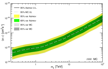
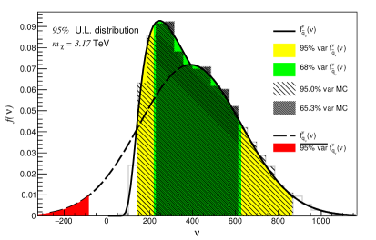
Figure 17: Left. Median and variance of upper limits (UL) from 1000 MC simulations (light dashed line and hatched areas) and analytic expressions based on the Asimov data set (solid black line and colored areas). Right. The solid line shows the distribution $f_{\tilde{q}_{\nu}}^{\nu}$ of $95\%$ upper limits as given in Eq. (A.5), for $m_{\chi}=1.6$ TeV, and the histogram shows the same quantity as derived from Eq. (5.8) used on MC data. As explained in the text, the skewness of the distribution is due to non-negative signals, $\nu\!\geq\!0$. Hatched bands show $68\%$ and $95\%$ quantiles of the MC simulations, respectably, while green and yellow areas show the corresponding quantities based on Eqs. (A.9, A.10). The dashed line, finally, corresponds to the distribution expected for an unconstrained signal strength parameter; here, the region colored in red indicates limits that are more than $2\sigma$ smaller than the mean expectation.

To confirm the validity of our analytic expressions based on the Asimov data set, we computed the upper limit on the signal strength at $95\%\,C.L.$ for 1000 MC data sets. These sets were generated as Poisson realizations of a power law with a spectral index of $-2.4$ and normalized to the total photon count of a GC simulation. In the left panel of Fig. 17, we show the median as well as 1 $\sigma$ and 2 $\sigma$ sidebands of these limits. For comparison, we also show these quantities as computed from Eqs. (A.8-A.10), with $\sigma_{A}$ estimated from the Asimov data set as $\sigma_{A}={\nu}\big{(}{{\tilde{q}_{\nu}}^{A,0}}\big{)}^{-1/2}$ for various pairs of $(\nu,\tilde{q}_{\nu})$ and $\tilde{q}_{\nu}=\text{TS}(\nu)$ as given in Eq. (5.7); here, the Asimov data set is treated as an ‘MC toy’ without any statistical fluctuations. Clearly, the agreement is excellent.

In the right panel of Fig. 17, we compare the distribution of $95\%$ upper limits found in the MC simulations (histograms) to the analytical expression in Eq. (A.5) (solid line), for a DM signal located at $m_{\chi}=1.6$ TeV. The skewness of the distributions is clearly visible and, again, the agreement is very good. For comparison, we also show with dashed lines the very different distribution that would result if the signal normalization could also be negative, i.e. Eq. (A.6). The area outside the $95\%\,C.L.$ of this distribution (marked in red) would in fact only cover negative signal normalizations.

A.4 Systematic uncertainty

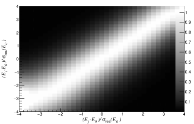
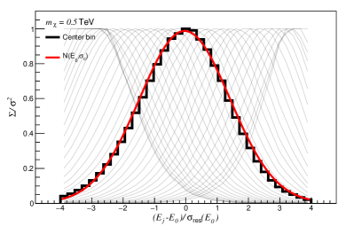
Figure 18: Left. The covariance matrix of Gaussian noise convoluted with the energy response matrix of CTAO, rescaled by the variance $\sigma$ of the noise. Photon energy bins $i,j$ are centered around the true mean energy $E_{0}$, which for the purpose of this plot we set to $E_{0}=0.5$ TeV, and stated in units of the energy resolution $\sigma_{\mathrm{res}}(E_{0})$ shown in Fig. 1. Right. The solid black line shows the center bin of the rescaled covariance matrix, $\Sigma/\sigma^{2}=\widetilde{M}\widetilde{M}^{T}$, and the red line is the best-fit normal distribution to approximate this function, with variance $\sigma_{c}=1.44$. For comparison, thin black lines show $(\widetilde{M}\widetilde{M}^{T})_{ij}$ for fixed bins $i$ that do not correspond to the central energy bin $E_{0}$.

In this Appendix we discuss i) the overall level of uncertainty and ii) the form of the covariance (or correlation) matrix $\Sigma_{ii^{\prime}}$ introduced in Eq. (5.4). Starting with the latter, we recall that this quantity is needed to account for systematic uncertainties due to noise correlations, cf. the likelihoods in Eqs. (5.5, 5.3) that we use in our analysis. We start from the energy response matrix $M_{ij}$, which is contained in the IRF in the form of a $2$-dimensional histogram describing the likelihood to reconstruct an energy (bin) $i$ as a function of true energy $j$, and normalize it as $\widetilde{{M}}_{ij}\equiv{M}_{ij}/\sum_{k}{M}_{kj}$. We then generate random noise vectors ${\bm{\epsilon}}$, with each of the components $\epsilon_{i}$ drawn from a normal distribution $N(0,\sigma)$ with variance $\sigma$, and convolute them with the normalized energy response matrix to give $\tilde{\bm{\epsilon}}\equiv\widetilde{{M}}{\bm{\epsilon}}$. We work under the assumption that observed photon counts ${\bm{\eta}}$ are subject to intrinsic fluctuations due to such Gaussian fluctuations, i.e. that they can be modelled as ${\bm{\eta}}=\langle{\bm{\eta}}\rangle+\tilde{\bm{\epsilon}}$. The covariance matrix thus becomes

$$\Sigma(\bm{{\eta}},\bm{{\eta}})\equiv\Big{\langle}(\bm{{\eta}}-\langle\bm{{\eta}}\rangle)(\bm{{\eta}}-\langle\bm{{\eta}}\rangle)^{T}\Big{\rangle}=\widetilde{M}\langle\bm{\epsilon},\bm{\epsilon}^{T}\rangle\widetilde{M}^{T}=\sigma^{2}\widetilde{M}\widetilde{M}^{T}\,,$$ (A.11)

which we show as a contour plot in the left panel of Fig. 18. For the purpose of this figure, we choose a central ‘pivot’ energy $E_{0}=0.5$ TeV to define bins $i=0$ and $j=0$.

In the right panel of the figure we directly plot $(\widetilde{M}\widetilde{M}^{T})_{ij}$ as a function of Energy $E_{j}$, for various discrete choices of $E_{i}$. We highlight (solid black line) the central bin distribution, i.e. $E_{i}=E_{0}$. As illustrated by the red line, the correlation matrix is very well fitted by a Gaussian, in this case with variance of $\sigma_{c}=1.46$ expressed in units of the energy resolution $\sigma_{\mathrm{res}}(E_{0})$ at energy $E_{0}$. We find that the best-fit value of this dimensionless variance only varies by an amount of the order of $10\%$ when considering different energies. Such variations do not have any significant impact on our sensitivity results, motivating us to consistently fix the correlation length at $1.5\times\sigma_{\mathrm{res}}$ as stated in Eq. (5.4).

We note in passing that the treatment of systematic uncertainties described here is complementary to the focus on mostly spatial correlations in the template fitting adopted in Ref. [7]. That analysis, in particular, is tailored to spatial pixels of the order of the PSF and energy bins somewhat larger than the energy resolution; in our analysis, on the other hand, the spatial bins are much larger than the PSF, and the energy bins are significantly smaller than the energy resolution.

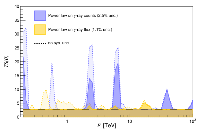
Figure 19: The value of the test statistic that is necessary to establish a $95\%$ upper exclusion limit for the two different background models described in the main text, for an assumed signal at energy $E_{0}$. These models describe, respectively, a power law on the total counts (blue) and only on the intrinsic gamma-ray spectrum (orange), which then is convoluted with the IRFs. Dotted lines show these values without assuming any systematic uncertainty in the analysis, while solid lines show the effect of adding an overall systematic uncertainty $\sigma$ at the indicated level. For comparison, the black dashed line shows the value expected for a $\frac{1}{2}\chi^{2}_{1}$ distribution. Results are based on $300$ MC toy simulations of the GC survey.

Let us now turn to the overall systematic uncertainty. As described in Sec. 5.3, we choose a value of 2.5 % for this quantity in order to correct for the fact that the test statistic, TS$(\nu)$, will realistically speaking not exactly follow the $\frac{1}{2}\chi^{2}_{1}$ distribution one expects if all signal (and background) components are modelled perfectly. Here we motivate this choice by computing the $95\%$ quantile of the TS$(0)$ distribution from a set of $300$ dedicated MC simulations of the GC analysis. In Fig. 19 we show the result for the two different background models described in Sec. 5.2, as a function of the monochromatic signal energy $E_{0}$. Concretely, these two models are given by a power law directly on the counts (blue) and a power law on the ‘intrinsic’ gamma ray spectrum (orange) that only afterwards is convoluted with the IRFs, respectively. Dotted lines show the results without including any systematic uncertainty, parameterized by the $\eta_{i}$ in the construction of the likelihoods outlined in Sec. 5.3, while solid lines show the effect of adding systematic uncertainty at the indicated level.

Compared to the expectation for a $\frac{1}{2}\chi^{2}_{1}$ distribution, namely a flat value of $2.71$, one can clearly identify several deviations. These can be traced back to the fact that the power-law assumption of the background is not perfect. Adding some level of overall systematic uncertainty to each of the counts smears out local deviations from a simple power law and therefore, as also clearly visible in the figure, leads to a reduction of these deviations. In other words, the larger the assumed statistical uncertainty, the more does the test statistic follow a $\frac{1}{2}\chi^{2}_{1}$ distribution (which we assume in the analysis, see also Appendix A.3). As expected, modelling only the intrinsic gamma-ray background as a power law (orange) provides a significantly better description of the counts. This, however, rests on the assumption of essentially perfect IRF modelling – which clearly is challenging to achieve in practice. Our benchmark analysis strategy therefore consists in being much more agnostic and instead modelling the total counts as a power law (blue). This leads to several deviations, most notably at $\sim 5$ TeV, where different spectral cuts in the transition region between MSTs and SSTs are expected to give rise to sharp variations in the spectrum (see also Fig. 4, right panel). We consider it sufficient to mitigate these deviations by introducing an overall uncertainty of $\sigma=0.025$, resulting in a TS distribution that only shows significant ($\gtrsim 4\,\sigma$) deviations around the mentioned $\sim 5$ TeV feature (which could be addressed by a dedicated treatment in the presence of real data). We also note that even an extremely conservative choice of $\sigma=0.05$ would at most decrease the estimated sensitivity by a factor of 2 at the lowest DM masses, cf. Fig. 13 in the main text.

References

- [1] Planck collaboration, Planck 2018 results. VI. Cosmological parameters, 1807.06209.
- [2] G. Jungman, M. Kamionkowski and K. Griest, Supersymmetric dark matter, Phys. Rept. 267 (1996) 195 [hep-ph/9506380].
- [3] G. Bertone, D. Hooper and J. Silk, Particle dark matter: Evidence, candidates and constraints, Phys. Rept. 405 (2005) 279 [hep-ph/0404175].
- [4] J. L. Feng, Dark Matter Candidates from Particle Physics and Methods of Detection, Ann. Rev. Astron. Astrophys. 48 (2010) 495 [1003.0904].
- [5] T. Bringmann and C. Weniger, Gamma Ray Signals from Dark Matter: Concepts, Status and Prospects, Phys. Dark Univ. 1 (2012) 194 [1208.5481].
- [6] https://www.cta-observatory.org/.
- [7] CTA collaboration, Sensitivity of the Cherenkov Telescope Array to a dark matter signal from the Galactic centre, JCAP 01 (2021) 057 [2007.16129].
- [8] CTA Consortium collaboration, Dark Matter and Fundamental Physics with the Cherenkov Telescope Array, Astropart. Phys. 43 (2013) 189 [1208.5356].
- [9] H. Silverwood, C. Weniger, P. Scott and G. Bertone, A realistic assessment of the CTA sensitivity to dark matter annihilation, JCAP 1503 (2015) 055 [1408.4131].
- [10] M. Pierre, J. M. Siegal-Gaskins and P. Scott, Sensitivity of CTA to dark matter signals from the Galactic Center, JCAP 1406 (2014) 024 [1401.7330].
- [11] CTA collaboration, Prospects for Indirect Dark Matter Searches with the Cherenkov Telescope Array (CTA), PoS ICRC2015 (2016) 1203 [1508.06128].
- [12] V. Lefranc, E. Moulin, P. Panci and J. Silk, Prospects for Annihilating Dark Matter in the inner Galactic halo by the Cherenkov Telescope Array, Phys. Rev. D91 (2015) 122003 [1502.05064].
- [13] M. Srednicki, S. Theisen and J. Silk, Cosmic Quarkonium: A Probe of Dark Matter, Phys. Rev. Lett. 56 (1986) 263.
- [14] L. Bergstrom and H. Snellman, Observable Monochromatic Photons From Cosmic Photino Annihilation, Phys. Rev. D 37 (1988) 3737.
- [15] L. Bergstrom, P. Ullio and J. H. Buckley, Observability of gamma-rays from dark matter neutralino annihilations in the Milky Way halo, Astropart. Phys. 9 (1998) 137 [astro-ph/9712318].
- [16] A. Ibarra, S. Lopez Gehler and M. Pato, Dark matter constraints from box-shaped gamma-ray features, JCAP 07 (2012) 043 [1205.0007].
- [17] T. Bringmann, L. Bergstrom and J. Edsjo, New Gamma-Ray Contributions to Supersymmetric Dark Matter Annihilation, JHEP 01 (2008) 049 [0710.3169].
- [18] T. Bringmann, X. Huang, A. Ibarra, S. Vogl and C. Weniger, Fermi LAT Search for Internal Bremsstrahlung Signatures from Dark Matter Annihilation, JCAP 07 (2012) 054 [1203.1312].
- [19] C. Weniger, A Tentative Gamma-Ray Line from Dark Matter Annihilation at the Fermi Large Area Telescope, JCAP 08 (2012) 007 [1204.2797].
- [20] H.E.S.S. collaboration, Search for Photon-Linelike Signatures from Dark Matter Annihilations with H.E.S.S., Phys. Rev. Lett. 110 (2013) 041301 [1301.1173].
- [21] Fermi-LAT collaboration, Updated search for spectral lines from Galactic dark matter interactions with pass 8 data from the Fermi Large Area Telescope, Phys. Rev. D 91 (2015) 122002 [1506.00013].
- [22] HESS collaboration, Searches for gamma-ray lines and ’pure WIMP’ spectra from Dark Matter annihilations in dwarf galaxies with H.E.S.S, JCAP 11 (2018) 037 [1810.00995].
- [23] HAWC collaboration, Search for gamma-ray spectral lines from dark matter annihilation in dwarf galaxies with the High-Altitude Water Cherenkov observatory, Phys. Rev. D 101 (2020) 103001 [1912.05632].
- [24] MAGIC collaboration, Search for Gamma-Ray Spectral Lines from Dark Matter Annihilation up to 100 TeV toward the Galactic Center with MAGIC, Phys. Rev. Lett. 130 (2023) 061002 [2212.10527].
- [25] ATLAS collaboration, Observation of a new particle in the search for the Standard Model Higgs boson with the ATLAS detector at the LHC, Phys. Lett. B 716 (2012) 1 [1207.7214].
- [26] CMS collaboration, Observation of a New Boson at a Mass of 125 GeV with the CMS Experiment at the LHC, Phys. Lett. B 716 (2012) 30 [1207.7235].
- [27] C. Weniger, T. Bringmann, F. Calore and G. Vertongen, Spectral cutoffs in indirect dark matter searches, J. Phys. Conf. Ser. 375 (2012) 012034 [1111.6998].
- [28] A. Ibarra, A. S. Lamperstorfer, S. López-Gehler, M. Pato and G. Bertone, On the sensitivity of CTA to gamma-ray boxes from multi-TeV dark matter, JCAP 09 (2015) 048 [1503.06797].
- [29] CTA Consortium collaboration, B. Acharya et al., Science with the Cherenkov Telescope Array. WSP, 11, 2018, 10.1142/10986, [1709.07997].
- [30] V. Lefranc, E. Moulin, P. Panci, F. Sala and J. Silk, Dark Matter in lines: Galactic Center vs dwarf galaxies, JCAP 09 (2016) 043 [1608.00786].
- [31] A. Hryczuk, K. Jodlowski, E. Moulin, L. Rinchiuso, L. Roszkowski, E. M. Sessolo et al., Testing dark matter with Cherenkov light - prospects of H.E.S.S. and CTA for exploring minimal supersymmetry, JHEP 10 (2019) 043 [1905.00315].
- [32] T. C. Weekes et al., Observation of TeV gamma rays from the Crab nebula using the atmospheric Cerenkov imaging technique, Astrophys. J. 342 (1989) 379.
- [33] R. Atkins et al., TeV gamma-ray survey of the northern hemisphere sky using the Milagro Observatory, Astrophys. J. 608 (2004) 680.
- [34] G. Di Sciascio, Ground-based Gamma-Ray Astronomy: an Introduction, J. Phys. Conf. Ser. 1263 (2019) 012003 [1904.06218].
- [35] https://www.mpi-hd.mpg.de/hfm/HESS/.
- [36] https://veritas.sao.arizona.edu/.
- [37] https://magic.mpp.mpg.de/.
- [38] A. Viana, H. Schoorlemmer, A. Albert, V. de Souza, J. P. Harding and J. Hinton, Searching for Dark Matter in the Galactic Halo with a Wide Field of View TeV Gamma-ray Observatory in the Southern Hemisphere, JCAP 12 (2019) 061 [1906.03353].
- [39] SWGO collaboration, The Southern Wide-field Gamma-ray Observatory, PoS ICRC2023 (2023) 963 [2309.04577].
- [40] Fermi-LAT collaboration, Fermi-LAT improved Pass~8 event selection, in 8th International Fermi Symposium: Celebrating 10 Year of Fermi, 10, 2018, 1810.11394.
- [41] DAMPE collaboration, Search for gamma-ray spectral lines with the DArk Matter Particle Explorer, Sci. Bull. 67 (2022) 679 [2112.08860].
- [42] H.E.S.S. collaboration, H.E.S.S. first public test data release, 1810.04516.
- [43] CTA Consortium collaboration, Introducing the CTA concept, Astropart. Phys. 43 (2013) 3.
- [44] T. Hassan et al., Monte Carlo Performance Studies for the Site Selection of the Cherenkov Telescope Array, Astropart. Phys. 93 (2017) 76 [1705.01790].
- [45] Fermi-LAT collaboration, The Large Area Telescope on the Fermi Gamma-ray Space Telescope Mission, Astrophys. J. 697 (2009) 1071 [0902.1089].
- [46] AGILE collaboration, The AGILE Mission, Astron. Astrophys. 502 (2009) 995 [0807.4254].
- [47] CTA Consortium collaboration, B. S. Acharya et al., Science with the Cherenkov Telescope Array. WSP, 11, 2018, 10.1142/10986, [1709.07997].
- [48] https://www.cta-observatory.org/science/cta-performance/.
- [49] J. Hisano, S. Matsumoto and M. M. Nojiri, Explosive dark matter annihilation, Phys. Rev. Lett. 92 (2004) 031303 [hep-ph/0307216].
- [50] C. Arina, T. Bringmann, J. Silk and M. Vollmann, Enhanced Line Signals from Annihilating Kaluza-Klein Dark Matter, Phys. Rev. D 90 (2014) 083506 [1409.0007].
- [51] A. Ibarra, D. Tran and C. Weniger, Indirect Searches for Decaying Dark Matter, Int. J. Mod. Phys. A 28 (2013) 1330040 [1307.6434].
- [52] F. Aharonian, D. Khangulyan and D. Malyshev, Cold ultrarelativistic pulsar winds as potential sources of galactic gamma-ray lines above 100 GeV, Astron. Astrophys. 547 (2012) A114 [1207.0458].
- [53] P. Ciafaloni, D. Comelli, A. Riotto, F. Sala, A. Strumia and A. Urbano, Weak Corrections are Relevant for Dark Matter Indirect Detection, JCAP 03 (2011) 019 [1009.0224].
- [54] G. Ovanesyan, T. R. Slatyer and I. W. Stewart, Heavy Dark Matter Annihilation from Effective Field Theory, Phys. Rev. Lett. 114 (2015) 211302 [1409.8294].
- [55] M. Baumgart, T. Cohen, I. Moult, N. L. Rodd, T. R. Slatyer, M. P. Solon et al., Resummed Photon Spectra for WIMP Annihilation, JHEP 03 (2018) 117 [1712.07656].
- [56] M. Baumgart, T. Cohen, E. Moulin, I. Moult, L. Rinchiuso, N. L. Rodd et al., Precision Photon Spectra for Wino Annihilation, JHEP 01 (2019) 036 [1808.08956].
- [57] M. Beneke, A. Broggio, C. Hasner and M. Vollmann, Energetic -rays from TeV scale dark matter annihilation resummed, Phys. Lett. B 786 (2018) 347 [1805.07367].
- [58] M. Beneke, A. Broggio, C. Hasner, K. Urban and M. Vollmann, Resummed photon spectrum from dark matter annihilation for intermediate and narrow energy resolution, JHEP 08 (2019) 103 [1903.08702].
- [59] M. Beneke, C. Hasner, K. Urban and M. Vollmann, Precise yield of high-energy photons from Higgsino dark matter annihilation, JHEP 03 (2020) 030 [1912.02034].
- [60] C. W. Bauer, N. L. Rodd and B. R. Webber, Dark matter spectra from the electroweak to the Planck scale, JHEP 06 (2021) 121 [2007.15001].
- [61] M. Beneke, K. Urban and M. Vollmann, Matching resummed endpoint and continuum -ray spectra from dark-matter annihilation, Phys. Lett. B 834 (2022) 137248 [2203.01692].
- [62] W.-L. Guo and Y.-L. Wu, Enhancement of Dark Matter Annihilation via Breit-Wigner Resonance, Phys. Rev. D 79 (2009) 055012 [0901.1450].
- [63] Y. Mambrini, A Clear Dark Matter gamma ray line generated by the Green-Schwarz mechanism, JCAP 12 (2009) 005 [0907.2918].
- [64] E. Dudas, Y. Mambrini, S. Pokorski and A. Romagnoni, Extra U(1) as natural source of a monochromatic gamma ray line, JHEP 10 (2012) 123 [1205.1520].
- [65] L. Bergstrom, T. Bringmann, M. Eriksson and M. Gustafsson, Gamma rays from Kaluza-Klein dark matter, Phys. Rev. Lett. 94 (2005) 131301 [astro-ph/0410359].
- [66] A. Birkedal, K. T. Matchev, M. Perelstein and A. Spray, Robust gamma ray signature of WIMP dark matter, hep-ph/0507194.
- [67] L. Bergstrom, T. Bringmann, M. Eriksson and M. Gustafsson, Gamma rays from heavy neutralino dark matter, Phys. Rev. Lett. 95 (2005) 241301 [hep-ph/0507229].
- [68] V. Barger, W.-Y. Keung and D. Marfatia, Bremsstrahlung in dark matter annihilation, Phys. Lett. B 707 (2012) 385 [1111.4523].
- [69] C. Garcia-Cely and A. Ibarra, Novel Gamma-ray Spectral Features in the Inert Doublet Model, JCAP 09 (2013) 025 [1306.4681].
- [70] T. Toma, Internal Bremsstrahlung Signature of Real Scalar Dark Matter and Consistency with Thermal Relic Density, Phys. Rev. Lett. 111 (2013) 091301 [1307.6181].
- [71] F. Giacchino, L. Lopez-Honorez and M. H. G. Tytgat, Scalar Dark Matter Models with Significant Internal Bremsstrahlung, JCAP 10 (2013) 025 [1307.6480].
- [72] L. Bergstrom, Radiative Processes in Dark Matter Photino Annihilation, Phys. Lett. B 225 (1989) 372.
- [73] G. Ovanesyan, N. L. Rodd, T. R. Slatyer and I. W. Stewart, One-loop correction to heavy dark matter annihilation, Phys. Rev. D 95 (2017) 055001 [1612.04814].
- [74] L. Rinchiuso, O. Macias, E. Moulin, N. L. Rodd and T. R. Slatyer, Prospects for Heavy WIMP Dark Matter with CTA: the Wino and Higgsino, 2008.00692.
- [75] GAMBIT Dark Matter Workgroup collaboration, DarkBit: A GAMBIT module for computing dark matter observables and likelihoods, Eur. Phys. J. C 77 (2017) 831 [1705.07920].
- [76] P. Gondolo and G. Gelmini, Cosmic abundances of stable particles: Improved analysis, Nucl. Phys. B 360 (1991) 145.
- [77] J. M. Cline, 130 GeV dark matter and the Fermi gamma-ray line, Phys. Rev. D 86 (2012) 015016 [1205.2688].
- [78] T. Bringmann, P. F. Depta, M. Hufnagel and K. Schmidt-Hoberg, Precise dark matter relic abundance in decoupled sectors, Phys. Lett. B 817 (2021) 136341 [2007.03696].
- [79] M. Winter, G. Zaharijas, K. Bechtol and J. Vandenbroucke, Estimating the GeV Emission of Millisecond Pulsars in Dwarf Spheroidal Galaxies, Astrophys. J. Lett. 832 (2016) L6 [1607.06390].
- [80] J. Knödlseder et al., GammaLib and ctools: A software framework for the analysis of astronomical gamma-ray data, Astron. Astrophys. 593 (2016) A1 [1606.00393].
- [81] J. Zavala and C. S. Frenk, Dark matter haloes and subhaloes, Galaxies 7 (2019) 81 [1907.11775].
- [82] A. Di Cintio, C. B. Brook, A. V. Macciò, G. S. Stinson, A. Knebe, A. A. Dutton et al., The dependence of dark matter profiles on the stellar-to-halo mass ratio: a prediction for cusps versus cores, Mon. Not. Roy. Astron. Soc. 437 (2014) 415 [1306.0898].
- [83] O. Y. Gnedin, A. V. Kravtsov, A. A. Klypin and D. Nagai, Response of dark matter halos to condensation of baryons: Cosmological simulations and improved adiabatic contraction model, Astrophys. J. 616 (2004) 16 [astro-ph/0406247].
- [84] J. Einasto, On the Construction of a Composite Model for the Galaxy and on the Determination of the System of Galactic Parameters, Trudy Astrofizicheskogo Instituta Alma-Ata 5 (1965) 87.
- [85] T. Bringmann, J. Edsjö, P. Gondolo, P. Ullio and L. Bergström, DarkSUSY 6 : An Advanced Tool to Compute Dark Matter Properties Numerically, JCAP 1807 (2018) 033 [1802.03399].
- [86] M. Hütten, C. Combet and D. Maurin, CLUMPY v3: -ray and signals from dark matter at all scales, 1806.08639.
- [87] J. F. Navarro, C. S. Frenk and S. D. White, The Structure of cold dark matter halos, Astrophys. J. 462 (1996) 563 [astro-ph/9508025].
- [88] Fermi-LAT collaboration, Measurement of the Cosmic Ray e+ plus e- spectrum from 20 GeV to 1 TeV with the Fermi Large Area Telescope, Phys. Rev. Lett. 102 (2009) 181101 [0905.0025].
- [89] D. Fegan, gamma/hadron separation at TeV energies, J. Phys. G 23 (1997) 1013.
- [90] F. Yusef-Zadeh, The Origin of the Galactic center nonthermal radio filaments: Young stellar clusters, Astrophys. J. 598 (2003) 325 [astro-ph/0308008].
- [91] F. Aharonian, R. Yang and E. de Oña Wilhelmi, Massive Stars as Major Factories of Galactic Cosmic Rays, Nature Astron. 3 (2019) 561 [1804.02331].
- [92] R. Genzel, F. Eisenhauer and S. Gillessen, The Galactic Center Massive Black Hole and Nuclear Star Cluster, Rev. Mod. Phys. 82 (2010) 3121 [1006.0064].
- [93] Fermi-LAT collaboration, Fermi-LAT Observations of the Diffuse Gamma-Ray Emission: Implications for Cosmic Rays and the Interstellar Medium, Astrophys. J. 750 (2012) 3 [1202.4039].
- [94] HESS collaboration, Characterising the VHE diffuse emission in the central 200 parsecs of our Galaxy with H.E.S.S, Astron. Astrophys. 612 (2018) A9 [1706.04535].
- [95] P. D. l. T. Luque, D. Gaggero, D. Grasso, O. Fornieri, K. Egberts, C. Steppa et al., Galactic diffuse gamma rays meet the PeV frontier, Astron. Astrophys. 672 (2023) A58 [2203.15759].
- [96] H.E.S.S. collaboration, Acceleration of petaelectronvolt protons in the Galactic Centre, Nature 531 (2016) 476 [1603.07730].
- [97] H.E.S.S. collaboration, Localising the VHE gamma-ray source at the Galactic Centre, Mon. Not. Roy. Astron. Soc. 402 (2010) 1877 [0911.1912].
- [98] H.E.S.S., NANTEN collaboration, Hess j1741 302 a hidden accelerator in the galactic plane, Astron. Astrophys. 612 (2018) A13 [1711.01350].
- [99] L. Herold and D. Malyshev, Hard and bright gamma-ray emission at the base of the Fermi bubbles, Astron. Astrophys. 625 (2019) A110 [1904.01454].
- [100] H.E.S.S. collaboration, Search for TeV emission from the Fermi Bubbles at low Galactic latitudes with H.E.S.S. inner Galaxy survey observations, PoS ICRC2021 (2021) 791 [2108.10028].
- [101] HESS collaboration, Searches for gamma-ray lines and ’pure WIMP’ spectra from Dark Matter annihilations in dwarf galaxies with H.E.S.S, JCAP 11 (2018) 037 [1810.00995].
- [102] H.E.S.S. collaboration, Search for dark matter signals towards a selection of recently-detected DES dwarf galaxy satellites of the Milky Way with H.E.S.S, 2008.00688.
- [103] J. D. Simon and M. Geha, The Kinematics of the Ultra-Faint Milky Way Satellites: Solving the Missing Satellite Problem, Astrophys. J. 670 (2007) 313 [0706.0516].
- [104] Fermi-LAT collaboration, Sensitivity Projections for Dark Matter Searches with the Fermi Large Area Telescope, Phys. Rept. 636 (2016) 1 [1605.02016].
- [105] R. M. Crocker et al., Gamma-ray emission from the Sagittarius dwarf spheroidal galaxy due to millisecond pulsars, Nature Astron. 6 (2022) 1317 [2204.12054].
- [106] Fermi-LAT collaboration, The spectrum of isotropic diffuse gamma-ray emission between 100 MeV and 820 GeV, Astrophys. J. 799 (2015) 86 [1410.3696].
- [107] M. Gilfanov, Low mass x-ray binaries as a stellar mass indicator of the host galaxy, Mon. Not. Roy. Astron. Soc. 349 (2004) 146 [astro-ph/0309454].
- [108] N. Mirabal, Dark matter vs. Pulsars: Catching the impostor, Mon. Not. Roy. Astron. Soc. 436 (2013) 2461 [1309.3428].
- [109] A. Gautam, R. M. Crocker, L. Ferrario, A. J. Ruiter, H. Ploeg, C. Gordon et al., Millisecond pulsars from accretion-induced collapse as the origin of the Galactic Centre gamma-ray excess signal, Nature Astron. 6 (2022) 703 [2106.00222].
- [110] M. B. Davies and B. M. S. Hansen, Neutron star retention and millisecond pulsar production in globular clusters, Mon. Not. Roy. Astron. Soc. 301 (1998) 15.
- [111] C. Y. Hui, K. S. Cheng and R. E. Taam, Dynamical Formation of Millisecond Pulsars in Globular Clusters, Astrophys. J. 714 (2010) 1149 [1003.4332].
- [112] R. de Menezes, F. Di Pierro and A. Chiavassa, How the dynamical properties of globular clusters impact their -ray and X-ray emission, Mon. Not. Roy. Astron. Soc. 523 (2023) 4455 [2306.03131].
- [113] E. Vasiliev and V. Belokurov, The last breath of the Sagittarius dSph, Mon. Not. Roy. Astron. Soc. 497 (2020) 4162 [2006.02929].
- [114] F. Calore, C. Eckner and S. Manconi, Assessing the gamma-ray emission from the Sagittarius dwarf spheroidal galaxy with adaptive template fitting and photon count statistics (in preparation), 2403.YYYYY.
- [115] CTA collaboration, In preparation, .
- [116] V. Bonnivard et al., Dark matter annihilation and decay in dwarf spheroidal galaxies: The classical and ultrafaint dSphs, Mon. Not. Roy. Astron. Soc. 453 (2015) 849 [1504.02048].
- [117] HESS collaboration, Search for -Ray Line Signals from Dark Matter Annihilations in the Inner Galactic Halo from 10 Years of Observations with H.E.S.S., Phys. Rev. Lett. 120 (2018) 201101 [1805.05741].
- [118] H.E.S.S. collaboration, Search for dark matter annihilations towards the inner Galactic halo from 10 years of observations with H.E.S.S, Phys. Rev. Lett. 117 (2016) 111301 [1607.08142].
- [119] A. Neronov and D. Semikoz, Mapping large-scale diffuse -ray emission in the 10100 TeV band with Cherenkov telescopes, Astron. Astrophys. 637 (2020) A44 [2001.00922].
- [120] A. Abdo et al., Fermi LAT Search for Photon Lines from 30 to 200 GeV and Dark Matter Implications, Phys. Rev. Lett. 104 (2010) 091302 [1001.4836].
- [121] Fermi-LAT collaboration, Fermi LAT Search for Dark Matter in Gamma-ray Lines and the Inclusive Photon Spectrum, Phys. Rev. D 86 (2012) 022002 [1205.2739].
- [122] HEGRA collaboration, Search for TeV gamma-ray emission from the Andromeda galaxy, Astron. Astrophys. 400 (2003) 153 [astro-ph/0302347].
- [123] T. Bringmann, F. Calore, G. Vertongen and C. Weniger, On the Relevance of Sharp Gamma-Ray Features for Indirect Dark Matter Searches, Phys. Rev. D 84 (2011) 103525 [1106.1874].
- [124] L. Bergstrom, G. Bertone, J. Conrad, C. Farnier and C. Weniger, Investigating Gamma-Ray Lines from Dark Matter with Future Observatories, JCAP 11 (2012) 025 [1207.6773].
- [125] J. Chang et al., An excess of cosmic ray electrons at energies of 300-800 GeV, Nature 456 (2008) 362.
- [126] CALET collaboration, Direct Measurement of the Cosmic-Ray Proton Spectrum from 50 GeV to 10 TeV with the Calorimetric Electron Telescope on the International Space Station, Phys. Rev. Lett. 122 (2019) 181102 [1905.04229].
- [127] DAMPE collaboration, Measurement of the cosmic-ray proton spectrum from 40 GeV to 100 TeV with the DAMPE satellite, Sci. Adv. 5 (2019) eaax3793 [1909.12860].
- [128] AMS collaboration, The Alpha Magnetic Spectrometer (AMS) on the international space station: Part II — Results from the first seven years, Phys. Rept. 894 (2021) 1.
- [129] “Ctao instrument response functions - prod5 version v0.1.” https://https://zenodo.org/records/5499840.
- [130] F. Calore, I. Cholis and C. Weniger, Background Model Systematics for the Fermi GeV Excess, JCAP 03 (2015) 038 [1409.0042].
- [131] V. Lefranc, G. A. Mamon and P. Panci, Prospects for annihilating Dark Matter towards Milky Way’s dwarf galaxies by the Cherenkov Telescope Array, JCAP 09 (2016) 021 [1605.02793].
- [132] Fermi-LAT collaboration, Searching for Dark Matter Annihilation from Milky Way Dwarf Spheroidal Galaxies with Six Years of Fermi Large Area Telescope Data, Phys. Rev. Lett. 115 (2015) 231301 [1503.02641].
- [133] Fermi-LAT collaboration, Searching for Dark Matter Annihilation from Milky Way Dwarf Spheroidal Galaxies with Six Years of Fermi Large Area Telescope Data, Phys. Rev. Lett. 115 (2015) 231301 [1503.02641].
- [134] J. Rico, Gamma-Ray Dark Matter Searches in Milky Way Satellites—A Comparative Review of Data Analysis Methods and Current Results, Galaxies 8 (2020) 25 [2003.13482].
- [135] W. A. Rolke, A. M. Lopez and J. Conrad, Limits and confidence intervals in the presence of nuisance parameters, Nucl. Instrum. Meth. A 551 (2005) 493 [physics/0403059].
- [136] F. James and M. Roos, Minuit: A System for Function Minimization and Analysis of the Parameter Errors and Correlations, Comput. Phys. Commun. 10 (1975) 343.
- [137] https://ph-root-2.cern.ch/.
- [138] G. Cowan, K. Cranmer, E. Gross and O. Vitells, Asymptotic formulae for likelihood-based tests of new physics, European Physical Journal C C71 (2011) 1554 [1007.1727].
- [139] Fermi-LAT collaboration, Updated search for spectral lines from Galactic dark matter interactions with pass 8 data from the Fermi Large Area Telescope, Phys. Rev. D 91 (2015) 122002 [1506.00013].
- [140] J. Hisano, S. Matsumoto, M. Nagai, O. Saito and M. Senami, Non-perturbative effect on thermal relic abundance of dark matter, Phys. Lett. B 646 (2007) 34 [hep-ph/0610249].
- [141] A. Hryczuk, R. Iengo and P. Ullio, Relic densities including Sommerfeld enhancements in the MSSM, JHEP 03 (2011) 069 [1010.2172].
- [142] T. Bringmann, E. Sæther Hatlen and G. Zaharijas, Likelihoods for the CTA sensitivity to a dark matter line signal from the Galactic centre (S. Abe et al., 2024]), Mar., 2024. 10.5281/zenodo.10792466.
- [143] P. Bechtle et al., Constrained Supersymmetry after two years of LHC data: a global view with Fittino, JHEP 06 (2012) 098 [1204.4199].
- [144] GAMBIT collaboration, Global fits of GUT-scale SUSY models with GAMBIT, Eur. Phys. J. C 77 (2017) 824 [1705.07935].
- [145] E. Bagnaschi et al., Likelihood Analysis of the pMSSM11 in Light of LHC 13-TeV Data, Eur. Phys. J. C 78 (2018) 256 [1710.11091].
- [146] H.E.S.S. collaboration, Search for Photon-Linelike Signatures from Dark Matter Annihilations with H.E.S.S., Phys. Rev. Lett. 110 (2013) 041301 [1301.1173].
- [147] P. D. Serpico and G. Zaharijas, Optimal angular window for observing Dark Matter annihilation from the Galactic Center region: the case of ray lines, Astropart. Phys. 29 (2008) 380 [0802.3245].
- [148] CTA Galactic Science Working Group collaboration, Survey of the Galactic Plane with the Cherenkov Telescope Array, PoS ICRC2021 (2021) 886 [2109.03729].