Empirical learning of dynamical decoupling on quantum processors

Abstract

Dynamical decoupling (DD) is a low-overhead method for quantum error suppression. We describe how empirical learning schemes can be used to tailor DD strategies to the quantum device and task at hand. We use genetic algorithms to learn DD (GADD) strategies and apply our method to the 27-qubit Bernstein-Vazirani algorithm, 5-qubit Grover’s algorithm, and 80-qubit mirror randomized benchmarking circuits. In each scenario, the GADD strategies significantly outperform canonical DD sequences. We demonstrate the generic and scalable nature of our GADD method in that it does not require a priori knowledge of target circuit outcomes and has runtime remaining constant with increasing circuit depth and qubit number. Moreover, the relative improvement of empirically learned DD strategies over canonical DD sequences is shown to increase with increasing problem size and circuit sophistication.

I Introduction

Dynamical decoupling (DD) [1, 2, 3, 4] is a well-established error suppression strategy that has improved quantum state fidelity in a wide variety of qubit platforms, including superconducting circuits [5, 6], trapped ions [7], solid state spins [8, 9, 10], and electron spins [11]. As programmable quantum computers are not yet fault tolerant [12, 13, 14, 15], suppression of errors is vital for useful quantum computation. DD has enabled state-of-the-art quantum computing demonstrations on superconducting qubit-based devices [16, 17, 18, 19], and may provide utility even in the fault-tolerant quantum computation regime [20].

DD was one of the earliest methods for quantum error suppression to be proposed, leading to a long history of DD design. In the past two decades, numerous novel and sophisticated DD sequences have been proposed. The majority of this work has been focused on canceling certain terms of the system-bath interaction, increasing the order in the pulse spacing $\tau$ to which errors are suppressed, or mitigating systematic errors in pulse implementation on a single qubit. We refer curious readers to Ref. [6] for a comprehensive survey of this work. However, the complexity of experimental-scale quantum circuits today has grown beyond the scale at which theoretical approaches to DD design have been considered. For example, universally robust DD (URDD) was proven to be robust to dephasing noise and systematic pulse errors in the single qubit case [21], but URDD and similar single-qubit robust sequences such as Eulerian DD (EDD) [22] have been applied to multi-qubit experiments [23, 24, 25]. Indeed, most of the DD sequences that are used in quantum computational experiments today [6] were derived to decouple single qubit systems from their surrounding environments. Although successful results are empirically observed, such DD sequences are not necessarily theoretically optimal as the single-qubit DD optimization neglects central sources of error in multi-qubit circuits such as quantum crosstalk [26]. While multi-qubit DD sequences exist, their application on quantum processors rarely succeeds [27] as multi-qubit quantum gates are substantially more error-prone than single-qubit ones [28]. Recently, staggered single-qubit DD sequences have been proposed for crosstalk suppression in multi-qubit systems [29]. However, such staggered sequences are difficult to implement because idle gaps on many qubits do not align by default. As the number of qubits increases, finding such alignments in the circuit timeline and computing the tradeoff between which crosstalk terms to cancel becomes highly non-trivial. More generally, the difficulty of designing a DD strategy that works under certain noise conditions and quantum control restrictions is compounded by the difficulty of accurately describing a device’s noise characteristics [28, 30].

The availability of quantum computers with fast interaction with classical computers has created the possibility of using classical optimization techniques to improve error suppression and mitigation [31]. Prime examples of this innovation include the probabilistic error cancellation [32], probabilistic error amplification [18], and readout error mitigation [33, 34, 35, 36], which have enabled state-of-the-art quantum computing experiments [18]. For error suppression, deep learning [37] and integration of CPMG [38, 39] and XY4 sequence placement with a variational quantum algorithm [40, 41] have been used to classically optimize effective DD strategies. We advance this work by providing a framework to empirically learn DD strategies tailored to the quantum device and task at hand. Our specific choice of the learning algorithm builds off of the work in Ref. [42], where the authors use a genetic algorithm to improve single-qubit quantum memory by considering a classical simulation of open quantum system dynamics. We generalize this approach by including empirical feedback from a bona fide quantum backend and expanding to multi-qubit circuits.

We start by reviewing DD in Sec. II. In Sec. III, we discuss the specific implementation of our learning scheme and the methods by which it explores the desired strategy space while maintaining computational tractability. In Sec. IV, we evaluate the performance of our method against current state-of-the-art DD methods on known quantum problems. Furthermore, we demonstrate the capability of our method to learn effective DD strategies on target quantum circuits with a priori unknown answers by employing easily simulable training circuits with a similar structure to the target quantum circuit. We demonstrate the ability of our method to increase the scale of existing large-scale benchmarking protocols on quantum processors. Finally, in Sec. V, we discuss the scope of applications for our GADD method and the implications of our results.

II Background on Dynamical Decoupling

We begin with a simplified framework of a noisy system that is typical of the context where DD sequences are theoretically analyzed. We consider an idle period of qubit evolution where the system dynamics are governed by a system-bath interaction $H_{SB}$ and bath-specific Hamiltonian $H_{B}$, such that for time $\tau$, the system evolution is given by the unitary operator

$$f_{\tau}=\exp[-i\tau(H_{SB}+H_{B})].$$ (1)

Let us consider the decoupling group $G$, a sub-group of unitary transformations $\mathrm{SU}(2)$, such that $g_{j}\in G$ acts on the system Hilbert space $\mathcal{H}_{S}$. The decoupling group acts on $f_{\tau}$ by conjugation:

$$\begin{split}g_{j}^{\dagger}f_{\tau}g_{j}&=\exp[-i\tau g_{j}^{\dagger}(H_{SB}+H_{B})g_{j}]\\ &=\exp[-i\tau(H_{SB}^{\prime}+H_{B})],\end{split}$$ (2)

where $H_{SB}^{\prime}=g_{j}^{\dagger}H_{SB}g_{j}$. For a general single-qubit system-bath coupling Hamiltonian

$$H_{SB}=\sum\limits_{\alpha=x,y,z}\sigma^{\alpha}\otimes B^{\alpha},$$ (3)

which implies that

$$H_{SB}^{\prime}=\sum\limits_{\alpha=x,y,z}\quantity(\sigma^{\alpha}+[g_{j}^{\dagger},\sigma^{\alpha}]g_{j})\otimes B^{\alpha}.$$ (4)

We consider the concatenation of $L-1$ such intervals of length $\tau$ conjugated by different elements $g_{j}\in G$. The corresponding unitary time evolution operator over time $T=(L-1)\tau$ is then

$$\begin{split}U(T)&=\prod_{j=1}^{L-1}g_{j}^{\dagger}f_{\tau}g_{j}\\ &=\exp[-i\tau\sum_{j=1}^{L-1}(H_{SB,j}^{\prime}+H_{B})+O(\tau^{2})]\end{split}$$ (5)

by the BCH formula, where $H_{SB,j}^{\prime}$ is effective Hamiltonian as derived in Eq. 4 due to conjugation by the $j^{\text{th}}$ element of the decoupling group present in the sequence. Such a time interval where the system evolves under $H_{SB}$ conjugated by elements of $G$ can be experimentally achieved by the length $L$ pulse sequence given by $p_{1}=g_{1}^{\dagger}$, $p_{L}=g_{L-1}$ and $p_{j}=g_{j-1}g_{j}^{\dagger}$ for $j=1,\dots,L-1$ at the corresponding times in the pulse sequence. As such, $G$ can be chosen such that the pulses $p_{j}$ are easily implemented from existing operations present on the quantum backend. Thus, performing DD requires nothing more than applying a pre-programmed sequence of pulses in parallel to the execution of any quantum computation. For example, taking $g_{1}=X$ from $G=\{I,X\}$ results in the $L=2$ pulse sequence $p_{1}=p_{2}=X$ and cancels all terms $H_{SB}$ not coupled to $\sigma^{x}$ to first order in $\tau$, while taking $g_{1}=X$, $g_{2}=Z$, $g_{3}=Y$ from $G=\{I,X,Y,Z\}$ results in the XY4 pulse sequence which cancels all system-bath interactions up to first order in the pulse spacing $\tau$ [6]. The selective cancellation of system-bath interactions with DD can be much more sophisticated, as exemplified by dynamically generated decoherence-free subspaces [4, 43, 27].

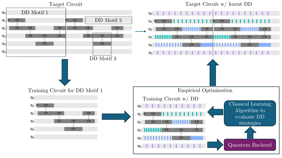
Fig. 1: The fast feedback between classical and quantum computers allows for the implementation of empirical methods for optimizing DD strategies. For a general training circuit with several different DD motifs, i.e. subcircuits in its circuit structure, an empirical DD optimization scheme can be run for any motif with an iterative quantum/classical approach. The output from independently optimizing DD on a motif can then be padded onto a specific target circuit.

We note that for a decoupling group of size $\absolutevalue{G}$ and pulse sequences of length $L$, there are $\binom{\absolutevalue{G}+L-2}{\absolutevalue{G}-1}$ equivalence classes of DD sequences distinguished by distinct $U(T)$ operators when neglecting contributions of $O(\tau^{2})$ and higher to the effective system-bath Hamiltonian. This result arises from counting the number of ways that the $L-1$ intervals where the system evolves under the effective Hamiltonian $g_{j}^{\dagger}H_{SB}g_{j}$ can be partitioned among the $\absolutevalue{G}$ possibilities for $g_{j}$. The equivalence class defined by maximal suppression to the first order of all terms in $H_{SB}$ anticommuting with all non-identity elements of $G$ is of particular theoretical interest. This class is achieved by selecting a permutation of the non-identity elements of $G$ to be the $\{g_{j}\}$ in the $L=\absolutevalue{G}$ case [44], of which there are $(L-1)!$. However, the equivalence of such sequences can be broken due to experimental gate implementations. For example, the sequences $XYXY$ and $YZYZ$ belong to this maximal suppression equivalence class for the decoupling group $G=\{I,X,Y,Z\}$. In various superconducting qubit-based devices, $X$ and $Y$ gates are implemented as finite width control pulses, while $Z$ is implemented as a virtual state rotation, leading to different behavior between the DD sequences $XYXY$ and $YZYZ$ [5, 6].

As a result, the number of distinct unitary transformations $U(T)$ that can experienced by a qubit in a programmable quantum computer when DD is applied is not restricted to the $\binom{\absolutevalue{G}+L-2}{\absolutevalue{G}-1}$ equivalence classes. Instead, it behaves much more like the upper bound of $\absolutevalue{G}^{L-1}$, where each $g_{j}$ can independently take on any element of $G$. Furthermore, in experimental-scale circuits with $N>1$ qubits, there can be $1\leq C\leq N$ independent DD sequences simultaneously applied to different qubits, giving an overall scaling of $\absolutevalue{G}^{(L-1)C}$. We show that it is possible to systematically search this large space and empirically identify well-performing DD strategies.

III Methods

III.1 Empirical learning of DD strategies

Given access to a programmable quantum device that can efficiently communicate with a classical device, the desired DD strategy can be found via empirical optimization using classical learning algorithms. To do so, we begin with a target circuit or a family of target circuits (Fig. 1) with potentially unknown outcomes a priori. We assume that the optimal DD strategy depends on the circuit structure defined by the position of the single qubit and entangling gates but not their specific parameters. To define the training circuits, we first define DD motifs, which are sub-circuit structures that are repeated in the target circuit. Examples of DD motifs are idle gaps on individual qubits, aligned idle gaps between neighboring qubits, three qubits with entangling operation on two qubits and idling on the third, and trivially, the training circuit itself. Previous comparisons of DD strategies on programmable quantum computers have focused on specific motifs: Ref. [6] discusses the wide array of methods for the idle gap motif in quantum memory experiments, Ref. [42] considers the motif of neighboring idle qubits on the backend graph and Ref. [26] considers crosstalk cancellation on the motif of qubits adjacent to an entangling operation. Notably, Ref. [40] considers the Cliffordized sub-circuit on a 4-qubit subset as its DD motif. In this work, we generalize to circuit-scale DD motifs unrestricted to simple idle gaps or small qubit clusters that are constructed by modifying certain circuit parameters while preserving general circuit structure. This is further discussed in Sec. III.3.

Equipped with the training circuit, the next step is to define a search space for the potential DD strategies and a way to navigate this space, i.e. the learning algorithm. Both continuous and discrete optimization methods are viable approaches. For continuous optimization, we can choose DD sequence parameters, such as pulse angle, duration, and spacing, which can be fed into continuous parameter optimization algorithms[45] like gradient-based methods or Nelder-Mead in a similar fashion to pulse-based variational strategies [46, 41]. In this work, we do not consider a continuous approach due to the large number of iterations and quantum-to-classical calls required for convergence in a space parameterized by continuous variables. We are hopeful that as quantum devices mature, we will see such variational DD strategies succeed. Instead, we consider discrete optimization with a genetic algorithm as our learning algorithm on the space of $C$ different length $L$ pulse sequences drawn from a given decoupling group $G$ on an $N$ qubit experimental-scale circuit. As discussed in the next subsection, our approach leads to a relatively quick convergence owing to the inherent parallelization of the genetic algorithm where individual DD strategies can be evaluated in parallel rather than sequentially. In particular, our technique is set apart from previous theoretical and empirical approaches to DD optimization in its scalability to quantum circuits with a large qubit number and circuit depth, as well as our ability to learn task-tailored DD strategies that address both system-environment as well as qubit-to-qubit crosstalk.

III.2 Genetic algorithms

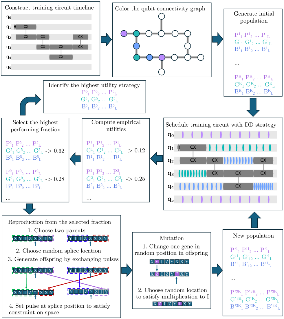
Fig. 2: Flowchart for searching effective DD strategies using genetic algorithm. Select qubits of the backend are 3-colored into $c=\{\text{P (Purple), G (Green), B (Blue)}\}$. Each individual in the initial population of size $K$ is associated with a PGB DD sequence. After utility functions are computed via empirical execution on the backend, they are used to select individuals for reproduction. Utility functions are then recursively computed on the resulting population of size $3K$ to select the new GA population. At any point, iteration can be terminated and the highest utility DD strategy selected for experimental application.

Genetic algorithms, inspired by evolution via natural selection, efficiently search a space of possibilities for individuals that optimize a given utility function, also called the objective function [47, 48]. In the prototypical genetic algorithm, an individual in a population can be identified by features analogous to genes on a chromosome. By identifying two individuals in the population and a scheme to exchange features among the two, additional individuals of the population can be generated in a process analogous to reproduction with genetic mutation.

The problem of determining DD strategies for a quantum circuit admits an unambiguous representation in the context of a genetic algorithm [42]. We begin by defining the space of DD strategies, which consist of applying different DD sequences to different qubits in a quantum circuit. As described in Sec. I, the space of DD strategies on an $N$-qubit quantum problem is characterized by the group of decoupling pulses $G$, the maximum number of pulses per sequence $L$, and the number of qubit sets $C$ that receive different single-qubit DD sequences. While there is a subtle difference between the decoupling group $G$ and the corresponding pulses $\{p_{j}\}$, the group structure of $G$ enforces that all $p_{j}\in G$. In this paper, we consider pulses from the group

$$G=\{I_{p},I_{m},X_{p},X_{m},Y_{p},Y_{m},Z_{p},Z_{m}\}$$ (6)

where $I_{p},X_{p},Y_{p},Z_{p}$ are the typical Pauli matrices and $I_{m},X_{m},Y_{m},Z_{m}$ are their respective equivalents with an additionally incurred global phase of $\pi$. This decoupling group was chosen to include most canonical DD sequences, such as XY4, EDD, and CPMG and its $X_{p}X_{m}$ variant, within the GADD search space, without incurring much additional overhead. $L$ is chosen depending on the typical length of qubit idle periods in a given quantum problem. Finally, we partition the $N$ circuit qubits into $C$ sets according to a graph where graph nodes represent circuit qubits and graph edges represent entangling gates between qubits present in the quantum circuit. This is similar to the connectivity graph of a device, except that we concern ourselves with only the present entangling operations in the specific circuit and neglect unused backend qubits. We color the vertices of the resulting graph using $C=2$ or $C=3$ colors such that no two vertices connected by an edge receive the same color and let each color receive an independent, uniformly spaced DD sequence. The sequence length $L$ is chosen such that idle periods in the target circuit are sufficiently long for the padding of $L$ pulses. In the case of staggered DD sequences, we impose that the first color has the pulse sequence placed uniformly between the operations defining the start and end of the idle period, while the second receives an asymmetric sequence with a pulse at the earliest time one can be applied in the idle period, and the third receives an asymmetric sequence with a pulse at the latest time one can be applied in the idle period. As the IBM heavy hexagon architecture is planar and cannot contain any subgraph isomorphic to $K_{4}$ [49], it is easy to find a $3$-coloring of the resulting graph such that no two vertices sharing an edge have the same color, and an analogous process can be performed on other limited-connectivity architectures. In the general case, our implementation is not restricted by the number of colors, where $C$ can be set to the number of qubits such that each qubit undergoes independent evolution. We note that we do not restrict ourselves to the equivalence class of DD sequences giving maximal suppression of errors to first order to allow for a more comprehensive search over different DD sequence staggerings for crosstalk mitigation. For a circuit partitioned into $C$ colors, our search space contains $2^{(L-1)C}$ distinct pulse staggerings, corresponding to the number of distinct ways to allocate $I\in G$ elements in each independent DD sequences.

The iterative optimization scheme employed by the GADD method is depicted in Fig. 2. After partitioning the qubits present in the circuit among the $C$ colors, we construct an initial population of $K$ DD strategies such that for each color $1\leq c\leq C$ and pulse location $1\leq l\leq L$, each element of $G$ appears an equal number of times (Appendix A). This is done to ensure that the GA convergence is driven by increases in utility rather than an initial bias towards any individual strategy. Then, each of the $K$ DD strategies is padded to the given quantum circuit and the resulting circuit is executed on the quantum computer for a fixed number of shots. For each strategy, we compute a utility function of the frequencies output by the projective measurement of the final state from the computer that is the target for optimization over the DD strategy space. Following the single-qubit reproduction scheme described in Ref. [42], after each utility function is computed, $K$ pairs of individuals are selected with replacement for reproduction to produce $2K$ offspring as described in Appendix C. The reproduction protocol can be defined for two pulse sequences

$$\begin{split}&c_{11}c_{12}\dots c_{1L}\\ &c_{21}c_{22}\dots c_{2L}\end{split}$$ (7)

by selecting a random site $l\in\{1,2,\dots,L\}$. Then, the offspring pulse sequences can be written as

$$\begin{split}c^{\prime}_{11}c^{\prime}_{12}\dots c^{\prime}_{1L}&\equiv c_{11}c_{12}\dots c*_{1l}c_{2(l+1)}c_{2(l+2)}\dots c_{2L}\\ c^{\prime}_{21}c^{\prime}_{22}\dots c^{\prime}_{2L}&\equiv c_{21}c_{22}\dots c*_{2l}c_{1(l+1)}c_{1(l+2)}\dots c_{1L},\end{split}$$ (8)

where $c*_{1l}$ and $c*_{2l}$ are selected to be the unique elements of $G$ that make the resulting sequences multiply to the identity. Furthermore, we implement the single-pulse where for each offspring $c^{\prime}$, where two pulse locations $1\leq l,l^{\prime}\leq L$ are selected. Then, $c^{\prime}_{l}$ is randomly mutated to some element of $G$ with a fixed probability, and $c^{\prime}_{l^{\prime}}$ is then constrained to again make the resulting sequence multiply to the identity. This protocol can be extended to DD strategies on $C$ qubit colors by performing single-qubit reproduction on each color, followed by a randomized assignment of the two single-color offspring to the two offspring strategies.

Finally, the utility function is re-computed for the $K$ parent and $2K$ offspring DD strategies, and $K/4$ highest utility parents and $3K/4$ highest utility offspring are chosen for the new population. The hyperparameters given as constants here were selected according to the values presented in Ref. [42]. The iterative process continues until convergence in the maximum value of the utility function has been reached and/or a sequence of desired utility has been discovered by the algorithm (Fig. 2). We note that the total GADD search space is equal to the upper bound on distinct DD sequences given in Sec. II. As the reproduction is defined for each color separately, each iteration of the genetic algorithm runs $C$ different DD sequences in parallel. While we can have $1\leq C\leq N$ for an $N$ qubit circuit, we choose $C$ as a balance between computational results (Sec. IV) and number of iterations required for convergence. We note that $C$ can only affect the number of iterations to converge, not the classical runtime of each GA iteration due to the independence of reproduction among colors. Furthermore, neither the width nor depth of the quantum circuit affects the overall GA runtime for constant $C$, contributing to the scalability of our method.

III.3 Training and target circuits

As the GA iterations are designed to learn DD strategies with high values for some utility function, selection of this utility function is key for training. When the output of a quantum problem is a deterministically known target state in the computational basis, we can simply select the success probability

$$p_{s}=\frac{\text{Number of target state measurements}}{\text{Number of total shots}}$$ (9)

to be the utility function to optimize. For example, this is relevant for the Bernstein-Vazirani problem where we construct an oracle encoding a bitstring of our choice as a first benchmark of the GADD method (Sec. IV.1).

However, generic quantum problems do not fall into this category. We overcome this challenge when given a general quantum task represented by a target circuit by constructing aforementioned training circuits which have a similar structure to the target circuit. After our GADD method learns a strategy with the desired utility on the training circuit, the strategy is applied to the target circuit. In this work, we consider circuit mirroring and Cliffordization as generic DD motif structure-preserving methods to construct training circuits and utility functions (Appendix B). When using the circuit mirroring method, we consider a target circuit with unknown outputs and then mirror the circuit by applying the inverse of the circuit gates at the end of the circuit in time reverse, which is a general technique with various applications as described in Ref. [50]. GADD can then be applied with the mirror circuit as a training circuit. If the time reversal echo cancels too many systematic errors to provide a useful signal for training, Ref. [50] details the method of inserting symmetry-breaking gates between the target circuit and its inverse block and then adjusting the circuit to keep the output easily simulatable. Under the Cliffordization method, one can create a training circuit by replacing all non-Clifford gates in the desired circuit with Clifford gates, and the resulting circuit is then efficiently simulable as the Clifford group acts as the stabilizer of the group of all unitary transformations on $N$ qubits [51]. We then construct our utility function to maximize

$$u(k)=1-\frac{1}{2}\sum_{k=0}^{2^{N}-1}\absolutevalue{f(k)-\hat{f}(k)}$$ (10)

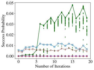
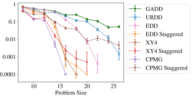
Fig. 3: Success probability for the Bernstein-Vazirani circuit on problem size 24 for one training session (left) and as a function of problem size for BV-8 to BV-26 (right) on ibm_peekskill. GADD is compared against a suite of established DD methods. Staggered sequences are represented by open diamonds and non-staggered sequences by open squares. Fluctuations of $\sim 1\%$ in the success probability are observed due to systematic backend performance fluctuations between GA iterations. The maximum success probability of finding the $1^{n}$ bitstring is evaluated across different values of $n$ (right) and GADD represents a significant improvement over all other tested DD methods.

where $f(k)$ is the simulated distribution of outcomes over the $2^{N}$ computational basis states $k$ on $N$ qubits and $\hat{f}(k)$ is the histogram estimator of the outcome distribution from projective measurements of the states from repeated executions of the training circuit on a programmable quantum backend.

IV Results and Discussion

We consider a variety of use cases of GADD to explore the scope of problems where an empirical search over the space of DD strategies yields a positive impact on computational results. These experiments exemplify three different choices for the utility function and three different training settings for GADD: success probability of the target circuit for Bernstein-Vazirani algorithm (Sec. IV.1), 1-norm of the Cliffordized probability distribution for Grover’s algorithm (Sec. IV.2), and success probability of smaller subcircuits from a representative random sample for mirror randomized benchmarking (MRB), a large-scale benchmarking protocol for programmable quantum computers (Sec. IV.3).

IV.1 Bernstein-Vazirani algorithm

The Bernstein-Vazirani (BV) algorithm was one of the first oracular quantum algorithms that was shown to demonstrate a theoretical quantum speedup [52]. In its conventional form, BV provides a linear quantum speedup over classical computation, and recently, an algorithmic quantum speedup was demonstrated in single-shot BV [25] via the use of URDD for error suppression. The existence of positive results with existing DD methods, as well as the linear scaling of the BV quantum circuit with problem size and deterministic target string, makes BV a standard choice for benchmarking protocols on programmable quantum devices  [53, 54, 55]. Here, we use the BV quantum circuit to compare the performance of GADD against a suite of well-established DD sequences commonly used in experimental settings today, including the symmetric and staggered versions of CPMG, XY4, and EDD, as well as URDD. In the staggered version, qubits of different colors experience staggered pulse timings, while URDD is not staggered as the URDD protocol selects pulse numbers based on idle duration lengths and thus has its own internal timing regulation [56].

BV-$n$ represents the BV problem where there exists a hidden bitstring $b\in\{0,1\}^{n}$ and the corresponding BV oracle outputs $f_{b}(x)=b\cdot x\pmod{2}$ when queried with the input bitstring $x$. The goal is to identify the hidden bitstring $b$ with the minimal number of oracle queries. The classical success probability after one iteration is $p_{\text{s,classical}}=2/2^{n}$ while the ideal quantum success probability is $p_{\text{s,quantum}}=1$ and requires $N=n+1$ qubits to implement. While there are $2^{n}$ different oracles in the BV-$n$ problem class, we choose to consider only the bitstring $b=1^{n}$ to be representative of the problem for each $n$ as it has the largest circuit depth, following the lead of Refs. [25, 53, 57]. These circuits are run on the 27-qubit ibm_peekskill backend with the IBM Falcon architecture. We consider the problem sizes $n=8,10,12,\dots,26$ up to the largest possible size on a 27-qubit device and repeat each circuit for 10,000 shots. The GADD experiment is performed with sequences with length $L=8$ for $20$ iterations and initial population with size $K=16$ with the probability of measuring the $1^{n}$ bitstring selected as the utility function. The GA mutation probability per offspring begins at 0.7 and increases by 0.1 if the spread of the DD sequence is more than 0.1 and decreases by 0.1 if the spread is less than 0.05.

First, we focus our attention on the convergence of the GADD algorithm in the $n=24$ case, which is characteristic of the GADD behavior on the BV problem in the larger $n$ regime (Fig. 3). We consider the highest success probability over strategies in the population at each iteration versus the iteration number to demonstrate the convergence of the GADD population to one with maximum success probability $0.04$ within $\sim 10$ iterations. This represents a more than $4$-fold increase in the success probability achieved with URDD and staggered CPMG, while all other sequences give success probability $p_{s}=0$.

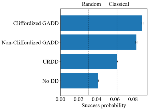
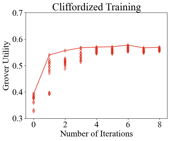
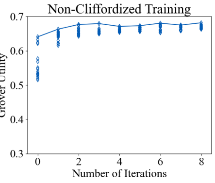
Fig. 4: 5-qubit Grover’s algorithm’s success probabilities averaged over all $2^{5}$ oracles (left) and the utility vs. iteration for GADD training on Cliffordized and non-Cliffordized, i.e. the original, Grover circuits (middle and right) on ibmq_mumbai. Here, the GADD was trained with the utility function relating to the difference from the ideal distribution as classical simulated. In both the Cliffordized (middle) and non-Cliffordized (right) training cases, we see the convergence of the GA within $\sim 5$ iterations. Iterations $9-20$ provide more iterations where the population has simply converged and is thus omitted. We note that for the non-Cliffordized circuit, our initial strategy population (Appendix A) happened to contain high-utility individuals. The average success probability (left) of GADD strategies from Cliffordized and non-Cliffordized training is higher than the URDD strategy and no DD strategy. The random threshold is established from a simple random uniform guess overall $2^{5}$ bitstrings, while the best classical strategy allows for a single classical query before guessing.

The general case in the large $n$ regime yields similar results upon comparing GADD with benchmark sequences. We find that our empirical method strikingly outperforms all theoretically derived sequences in the test suite (Fig. 3). For comparison, in the smaller problem sizes regime of $n\lessapprox 16$, we find that both GADD and URDD have high success probabilities, reproducing previous work that empirically demonstrated good error suppression with URDD [6, 25, 23]. The relative improvement of empirically learned GADD strategies over URDD increases with problem size, and the success probability obtained via GADD achieves a much slower decay of $p_{s}$ with respect to problem size $n$ when compared to all other DD strategies in our test suite.

We further note some particularly interesting results from the DD test suite. The staggered DD sequences did not have generic improvements in DD performance with respect to the non-staggered sequences. As explained in Appendix D, this is an example of a generic phenomenon where DD sequences optimized for single-qubit decoupling may not perform well in experimental-scale quantum circuits with a vast sample of different gate timings. Another interesting result was that robust DD sequences like EDD did not necessarily exhibit higher computational fidelities than non-robust sequences like CPMG and XY4. This is not necessarily unexpected as these sequences are only robust under certain single-qubit pulse imperfections, like flip-angle errors, which may not be the most prominent error source for the chosen device. On the other hand, URDD was constructed to be robust to a broader variety of errors, has the inherent pulse timing selection functionality, and performed quite well with respect to the other methods in the suite.

Although it may be possible that there can be further improvement in the DD performance with continuous pulse spacing optimization or further hyperparameter tuning in GADD or other methods such as URDD, such an improvement necessitates a computational tradeoff over this convergence rate. Additionally, the improvements in computational fidelity due to DD can be limited by the difference between our GADD performance and the theoretical Markovian limit as DD is only effective against non-Markovian errors [58]. Most pertinently, the ability of GADD to learn DD strategies that match and exceed the performance of sequences in the test suite, each of which resulted from insightful theoretical analyses, highlights that the task of DD design can be outsourced to empirical learning algorithms.

IV.2 Grover’s algorithm

Next, we consider Grover’s search algorithm, where the underlying circuit and the utility function are more sophisticated than the BV algorithm. Grover’s search algorithm seeks to find a hidden length $N$ bitstring $b$ in an unsorted list with $2^{N}$ elements. The oracle in Grover’s algorithm returns $f_{b}(x)=\delta_{x,b}$ when queried with the input bitstring $x$. Classically, searching such an unsorted list requires $O(N)$ queries. By encoding the problem in an $N$ qubit circuit, a quadratic improvement in the number of queries is provably achieved relative to the best possible classical algorithm [59]. However, even for relatively small $N$, the circuit depths associated with even the most efficient implementations of Grover’s algorithm do not exhibit better-than-classical results without DD due to errors [24].

Grover’s search algorithm provides an ideal platform to evaluate the concept of Cliffordized training for two reasons. First, there are $2^{N}$ Grover search problems on $N$ qubits that can be easily accessed by changing specific parameters in non-Clifford gates present in the Grover oracle, but without changing the general circuit structure. Second, the depth of the Grover circuit imposes that although the $N=5$ case poses challenges in terms of error on the quantum backend, it is sufficiently small for individual non-Clifford Grover circuits to be tractably simulated classically. As a result, the effects of training with a Cliffordized circuit can be effectively compared with the effects of training with the circuit before Cliffordization.

We begin by considering two different training circuits for GADD. First, we consider the Cliffordized version of the Grover circuit encoding target bitstring $11111$, as well as its original non-Cliffordized form as a control to evaluate the effect of Cliffordization. For each of these circuits, we run the GADD algorithm for DD strategies with the same hyperparameters as in the BV problem, except with utility function $u(t)$ which considers total absolute difference between the simulated and experimentally estimated distribution of output counts in the computational basis with $N=5$ qubits as described in Eq. 10 over $4000$ shots. We note that this utility function has no knowledge of what the Grover target string is in the Cliffordized case. The resulting learned DD sequence is then padded to all $32$ distinct circuits for $N=5$ Grover search problems and the average search success probability over the $32$ circuits is calculated. These circuits are run on the 27-qubit ibmq_mumbai backend, which is a superconducting qubit device with the IBM Falcon architecture.

In both the Clifford and non-Clifford training cases, we observe convergence in the population generated by GADD after $\sim 4$ GA iterations (Fig. 4). After implementing these learned high-utility DD strategies on all $N=5$ Grover circuits, we demonstrate that significantly better-than-classical success probabilities are achieved under the implementation of GADD under both training cases as depicted in the right panel of Fig. 4. In contrast, this is not achieved in the case where URDD, the strategy that generically gave the next highest performance in Sec. IV.1, is implemented. Notably, the Grover success probability is comparable in the Cliffordized and non-Cliffordized training cases, which provides empirical evidence for the effectiveness of GADD training on a result-agnostic utility function. As the Cliffordized circuit provides a more general representation of the $N=5$ qubit Grover problem overall Grover oracles, while the non-Clifford circuit preserves the non-generalizable information of $11111$ being the target string, the comparable resulting Grover success probabilities imply that encoding such output-dependent information in the GADD utility function is unimportant. Thus, the Cliffordization method for generating training circuits is quite promising for learning successful DD strategies in the general setting where the resulting quantum state from the problem at hand is a priori unknown.

IV.3 Mirror randomized benchmarking

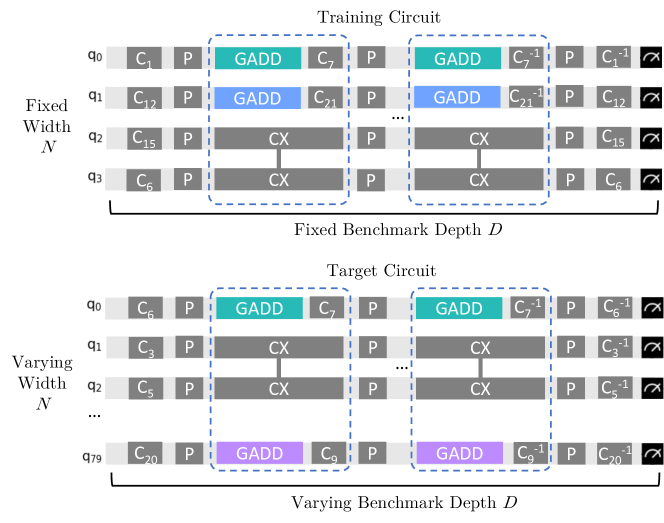
Fig. 5: Prototypical Clifford MRB circuits [60] for training and target circuits. $D/2$ layers (dashed boxes) of single-qubit Clifford gates and CNOTs are mirrored ($C_{n}$ and $C_{n}^{-1}$) across the circuit for a total of $D$ benchmark layers, and each has temporal gaps from the difference in one- and two-qubit gate times that enable the insertion of short GADD sequences. Uniformly random layers of Paulis ($P$) dress the benchmark layers and there are two mirrored layers of single-qubit Cliffords at the start and end. While training circuits (top) are fixed in the number of qubits $N$ and benchmark depth $D$, the target circuits (bottom) can vary in $N$ and $D$. Because of the randomized nature of the circuits, the location of two-qubit gates and gaps vary between each circuit.

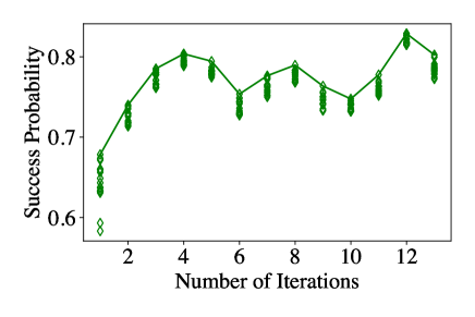
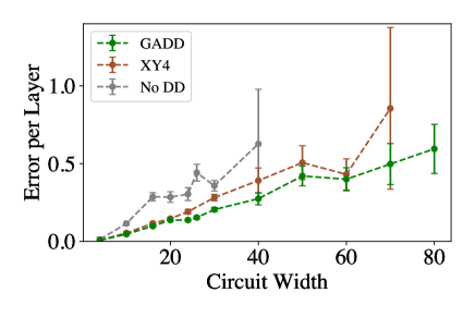
Fig. 6: MRB training circuits success probability as a function of the number of iterations (top), showing a quick convergence to the maximal utility, and final MRB results (bottom), both on ibm_kyiv. EPL calculations at different numbers of qubits with No DD, XY4, and the best-performing GADD sequence. Points with large error bars result from poor EPL curve fits due to a lack of signal at the limit of scalability. This breakdown point is achieved between 30-40 qubits without DD. Upon addition of the XY4 DD strategy, this breakdown point is moved to the 60-70 qubit regime but is observed at 80 qubits upon implementation of the strategy learned by GADD.

Mirror randomized benchmarking (MRB) is a scalable variant of the standard randomized benchmarking (RB) [61, 62] protocol that characterizes the noise of quantum processors by measuring the error rates of randomized layers sampled from a defined gate set [60, 63]. In Clifford MRB [60], $D$ benchmark layers of single-qubit Clifford gates and two-qubit gates are inverted and reflected across the central time axis of the circuit. Layers of random Pauli gates dress each of the benchmark layers and a single-qubit Clifford layer and its inverse are applied at the start and end of the protocol respectively (Fig. 5). In the universal version of the protocol that uses gates sampled from a universal gate set such as $\mathrm{SU}(2)$, composite layers are constructed by randomly sampling single-qubit unitary gates from $\mathrm{SU}(2)$ with a specified density of two-qubit entangling gates, and the second half of the circuit is the inverse of the first half randomly compiled to prevent systematic error cancellation [63]. In either protocol, mirror circuits are run on a processor and then an effective polarization $S$, a weighed success probability, is calculated for each $N$-qubit circuit as derived in Ref. [60]:

$$S=\frac{4^{N}}{4^{N}-1}\left[\sum_{k=0}^{N}\left(-\frac{1}{2}\right)^{k}h_{k}\right]-\frac{1}{4^{N}-1},$$ (11)

where $h_{k}$ is the probability that the circuit output bitstring is Hamming distance $k$ from the target bitstring.

The error per layer (EPL) is then calculated by fitting an exponential decay curve, $Ap^{D}$, to the relation of $S$ versus the benchmark depth $D$:

$$\text{EPL}=\frac{2^{N}-1}{2^{N}}\left(1-p\right),$$ (12)

which corresponds to the average gate infidelity of the Pauli-dressed $N$-qubit benchmark layer.

While MRB is more scalable than standard RB, which is infeasible beyond five qubits [60], it still has difficulty scaling to the 50+ qubits regime on current superconducting hardware, where other benchmarks such as layer fidelity [64] must be used instead. The difficulty is mainly due to crosstalk [63, 65] as the number of qubit-qubit entanglements increases linearly with the number of circuit qubits. On the other hand, the individual gates that MRB is intended to benchmark typically have similar error rates across an entire device, so the EPL per qubit is expected to remain roughly constant in the crosstalk-free regime. As a result, there exists a threshold number of qubits above which a nonzero effective polarization cannot be calculated even for the smallest circuit depths due to noise. We are therefore interested in examining whether it is possible to increase the scalability of MRB on real devices by increasing the average effective polarization of a randomized MRB circuit in the 50+ qubits regime.

MRB is an interesting test case for the efficacy of GADD for multiple reasons. First, the condensed idle periods between layers in a typical MRB circuit are sufficiently short such that longer robust sequences cannot be padded; the previous effort to improve the signal-to-noise used simple CPMG sequences [65]. Second, the nature of attempting to extend the benchmark to larger numbers of qubits necessitates using training circuits over smaller numbers of qubits, since the full-size target circuit will likely not have enough signal-to-noise to train on (Fig. 5). Third, the randomized nature of MRB circuits implies the training and target circuits must be fully random and not share repeating motifs even for a constant number of qubits. Therefore, to succeed, GADD must find sequences that lower error rates on small motif circuits with relatively small idle gaps for DD insertion and also lower error rates on larger circuits with slightly different gates and timings due to the randomized nature of MRB circuits. As a result, MRB represents one of the most general and challenging settings for applying learned DD sequences on training circuits to target circuits.

With these points in mind, we choose Clifford MRB as our problem and perform our GADD algorithm on strategies with $L=4$ sequences across the 127-qubit ibm_kyiv backend, which is a superconducting qubit device with the IBM Eagle architecture. We use subsets of linear qubit arrays, which only require two different colors alternating on adjacent qubits. To train the GADD algorithm, we calculated the utility function by computing the average success probability over a fixed set of $5$ random MRB circuits on 10 qubits containing $6$ circuit layers. CNOT was used as the two-qubit gate of choice on the layers sampled with the edge grab sampler [50] with a two-qubit gate density $0.25$. The convergence to the asymptotic maximal utility, as shown in Fig. 6, happened quickly within five iterations, similar to the training in the previous Bernstein-Vazirani and Grover’s settings. The DD strategy giving the highest success probability after training was then padded across a suite of random MRB circuits at varying benchmark depths to fit the effective polarization to an exponential and extract the EPL. These circuits were also run without DD and with the XY4 sequence on the same qubits for comparison.

The results are shown in Fig. 6. While MRB circuits on $\sim$40 qubit linear strings without dynamical decoupling already fail to produce any useful signal, XY4 was able to extend the range to $\sim$60 qubits, and the best GADD strategy learned via training extends the range to $\sim$80 qubits. Note that while we do report a value at 70 qubits for XY4, the underlying data is quite noisy and the corresponding EPL error bars are large. The increased range also corresponds to reduced average error per layer as DD effectively reduces crosstalk contributions. This demonstrates the effectiveness of GADD on randomized circuits even when training on motif circuits far smaller than the desired target circuit and its potential for extending the scalability of such protocols, including, but not limited to, $\mathrm{SU}(2)$ universal MRB. These results suggest that as long as the circuit structure of the motif resembles that of the final circuit, it is possible for the GADD training procedure to find a DD strategy that achieves results with lower errors and greater scalability beyond using canonical DD sequences.

V Conclusion

DD sequences are known to perform well on simple DD motifs such as that present in quantum memory preservation, where qubits experience a fixed time delay between the preparation and measurement with no gate operations. As a result, many implementations of DD in experimental-scale quantum computing experiments simply involve the placement of single-qubit sequences that perform well for memory preservation within idle gaps of more sophisticated circuits. Recently, this idea has been extended to analyze crosstalk when accounting for entanglement in analogous multi-qubit quantum memory experiments [27, 26]. The theoretical sophistication needed to model the effect of DD on crosstalk is a precursor to a proper analysis of DD on sophisticated circuits with general multi-qubit correlations and varied gate timings. Empirical methods such as Ref. [40] took positive steps in addressing this complexity by varying DD placement empirically and considering Cliffordized 4-qubit subcircuit motifs. Here, we provide a substantial extension of these ideas by allowing for empirical optimization on any circuit structure and exponentially many DD strategies. The performance of empirically optimized DD strategies should be judged on the two progressively difficult criteria of matching and exceeding the performance of robust DD sequences derived in the quantum memory setting. With the large size and relatively unknown structure of the general DD strategy space, matching the performance of well-studied robust sequences is in itself a worthy goal. Our results demonstrate the satisfaction of both criteria across all investigated experimental applications.

Learning effective error suppression strategies requires a systematic method to search the space of possible DD strategies. In this paper, we present an empirical method for doing this. To exemplify the empirical learning strategy, we use a genetic algorithm to search for well-performing DD strategies over all possible uniformly spaced DD sequences of length $L$ on $C$ independent qubit groups constructed from a decoupling group of size $\absolutevalue{G}$. We described how easy-to-train proxy circuits can be generated from sophisticated target circuits, which can then be trained using target-agnostic utility functions. Our strategy repeatedly performed better than current state-of-the-art DD techniques on several quantum tasks. In particular, we show that GADD sequences perform significantly better than canonical DD strategies when solving the 27-qubit Bernstein-Vazirani and 5-qubit Grover search problems. We also report the first MRB results at the 80-qubit regime, where other error suppression strategies had failed to yield useful results.

While our learning strategy is noise-aware, the computational overhead associated with learning does not increase with increasing qubit number or circuit depth. Not only is such a learn-as-you-run strategy more efficient than using noise calibration to design error suppression, it also enables better noise benchmarking of the devices, as evidenced by our MRB results. Studying strategies discovered via empirical DD learning could also be used to learn noise profiles and pulse imperfections of quantum devices. We expect that other optimization techniques, beyond genetic algorithms, can be applied for similar purposes and perhaps to find more DD sequences of theoretical interest.

Appendix A Starting population

We construct a uniform initial population of DD strategies by ensuring that for each qubit subset, each pulse appears at each site the same number of times. For example, one initial population of $Q=16$ DD strategies for $L=8$ DD sequences with the decoupling group $G=\{I_{p},I_{m},X_{p},X_{m},Y_{p},Y_{m},Z_{p},Z_{m}\}$ applied to a 3-colored qubit graph consists of following set of sequences, each of which is applied to all qubit colors:

• $I_{p}I_{m}X_{p}X_{m}Y_{p}Y_{m}Z_{p}Z_{m}$

• $I_{p}X_{p}Y_{p}Z_{p}I_{m}X_{m}Y_{m}Z_{m}$

• $I_{m}X_{p}X_{m}Y_{p}Y_{m}Z_{p}Z_{m}I_{p}$

• $X_{p}Y_{p}Z_{p}I_{m}X_{m}Y_{m}Z_{m}I_{p}$

• $X_{p}X_{m}Y_{p}Y_{m}Z_{p}Z_{m}I_{p}I_{m}$

• $Y_{p}Z_{p}I_{m}X_{m}Y_{m}Z_{m}I_{p}X_{p}$

• $X_{m}Y_{p}Y_{m}Z_{p}Z_{m}I_{p}I_{m}X_{p}$

• $Z_{p}I_{m}X_{m}Y_{m}Z_{m}I_{p}X_{p}Y_{p}$

• $Y_{p}Y_{m}Z_{p}Z_{m}I_{p}I_{m}X_{p}X_{m}$

• $I_{m}X_{m}Y_{m}Z_{m}I_{p}X_{p}Y_{p}Z_{p}$

• $Y_{m}Z_{p}Z_{m}I_{p}I_{m}X_{p}X_{m}Y_{p}$

• $X_{m}Y_{m}Z_{m}I_{p}X_{p}Y_{p}Z_{p}I_{m}$

• $Z_{p}Z_{m}I_{p}I_{m}X_{p}X_{m}Y_{p}Y_{m}$

• $Y_{m}Z_{m}I_{p}X_{p}Y_{p}Z_{p}I_{m}X_{m}$

• $Z_{m}I_{p}I_{m}X_{p}X_{m}Y_{p}Y_{m}Z_{p}$

• $Z_{m}I_{p}X_{p}Y_{p}Z_{p}I_{m}X_{m}Y_{m}$

At any given index of the pulse sequence, each element $g_{j}\in G$ is present at the same nonzero frequency. As a result, there is no artificial initial preference of the GA population for any individual pulse to take on any specific $g_{j}$ over other elements of $G$. We evaluate this method of constructing a uniform initial population by simulating the exploration of the genetic algorithm in the space of length 8 DD sequences when the utility associated with each sequence is uniformly selected at random on $[0,1]$ to characterize how the GA explores sequences when it is agnostic of a utility function landscape. Since the DD sequence associated with any color evolves independently of other colors, this simulation is indicative of the effectiveness of the DD strategy space exploration. A simulation demonstrates that in 7 GA iterations (Fig. 7), more of the DD strategy space is explored starting from the uniform population than a random starting population in expectation at any mutation probability and higher mutation probabilities lead to smaller differences between the behaviors of the two in terms of number of unique strategies explored as expected. This benefit is particularly important when a real optimization landscape with DD utilities is imposed, as exploring a larger fraction of the parameter space at any iteration number leads to lower probabilities of converging to local extrema that are suboptimal compared to a globally optimal DD strategy.

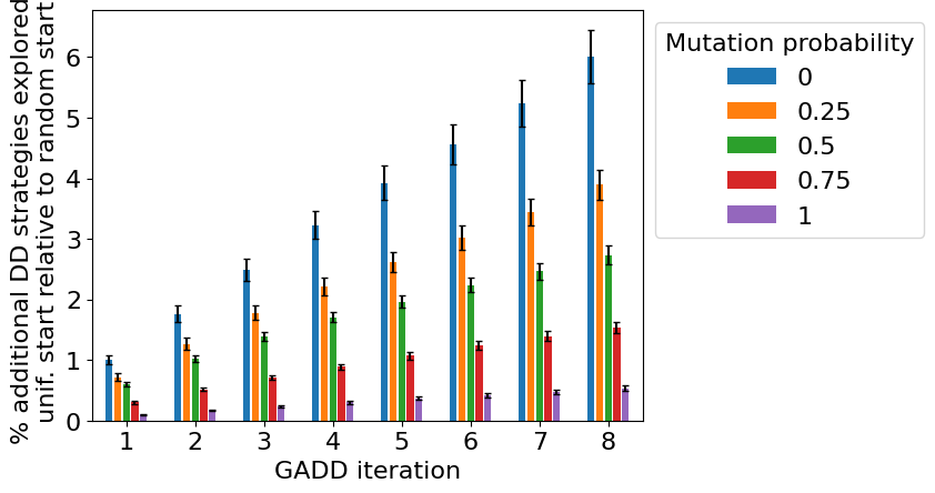
Fig. 7: The GADD algorithm with $C=1$ was used to explore the space of DD strategies on $G=\{I_{p},I_{m},X_{p},X_{m},Y_{p},Y_{m},Z_{p},Z_{m}\}$ with utility functions assigned uniformly at random to all strategies in the case of the example uniform starting population and $25$ different randomly selected populations of $L=8$ strategies. At each iteration, all pairs of DD strategies underwent reproduction to characterize the number of strategies that can theoretically be explored at that iteration number. Then, to maintain computational tractability, a random sample of 100 sequences was selected to be the new population. For each mutation probability, the average total number of DD sequences that can be explored in the random initial population case is compared relative to the average total number of DD sequences that can be explored in the uniform case. We find that at all GADD iteration numbers and mutation probabilities, starting the simulation from the example uniform starting population leads us to explore a larger amount of the DD strategy space compared to starting from a typical random population.

Appendix B Creating Cliffordized circuits

For quantum circuits with a priori unknown outputs, we can reduce the problem to the known output case by constructing a training circuit whose outputs are known via simulation by classical methods. The resulting obtained optimal DD strategy can then be padded on the original circuit to obtain GADD error-suppressed results. One method that we use to alter the circuit to obtain a well-defined utility function is through Cliffordization, where all non-Clifford gates in the circuit transpiled in terms of the native backend gates are replaced with native backend gates that belong to the Clifford group. Generically, for quantum gate $U$ imparting phase $0\leq\phi\leq\frac{\pi}{2}$, $\phi$ is set to $\frac{\pi}{2}$ with probability $\frac{\phi}{\pi/2}$ and $0$ with the remaining probability. Analogously, this conversion is performed for $\phi\in(\frac{\pi}{2},\pi),(\pi,\frac{3\pi}{2}),(\frac{3\pi}{2},2\pi)$ with their respective bounds. If $U$ also imparts a bit flip, the bit flip is converted into a phase rotation by the Hadamard gate, the previous protocol is applied to the phase rotation, and the resulting Clifford phase rotation is converted back into a bit flip with another Hadamard gate. For example, the $T^{{\dagger}}$ gate imparting a $\frac{-\pi}{4}$ phase on a quantum state in the computational basis can be Cliffordized by replacing it with a gate with $\phi=\frac{3\pi}{2}$ or the identity with $\phi=0$ with equal probability. The resulting circuit can then be simulated in polynomial time in the number of computational qubits according to the stabilizer circuit method [51]. The utility of this method, which we demonstrate in Sec. IV.2, relies on the ansatz that non-Markovian errors on the DD timescale are dependent on the general circuit structure (i.e. the location and approximate timing of gates in the transpiled circuit), but not necessarily the exact parameters associated with each gate.

Appendix C Reproduction and mutation

We begin with an initial population of DD strategies with size $K$, we select $K$ pairs of strategies for reproduction independently with replacement. The probability that any individual is selected for reproduction is proportional to the logarithm of its utility calculated from the previous genetic algorithm iteration. This construction follows the one used in Ref. [42] with the goal of converging towards the highest utility DD strategies, due to both the survival of high utility DD strategies across GA iterations and the increased probability of selecting high utility DD strategies for reproduction.

For each new strategy generated by reproduction, the single pulse mutation occurs with some probability that is fixed per GA iteration but can vary throughout iterations of the genetic algorithm. This dynamic variation of the mutation probability is designed to accelerate the convergence of the genetic algorithm to the desired result. We find good convergence in the aforementioned results by initially setting the mutation probability to around $0.7$ and dynamically increasing or decreasing the mutation probability by $0.1$ if the system appears to be far away or close to equilibrium respectively. Due to the complicated DD optimization landscape, the state of being in or out of equilibrium is difficult to quantify via iteration snapshots. We find that using proxy quantities such as the standard deviation or range of utility functions exhibited by all individuals in the population at any individual GA iteration gives reasonably good convergence results. However, such a condition is significantly dependent on the problem structure and utility function selection and there has not been sufficient rigorous testing for attribution of varying mutation rates to varying convergence.

Strategy	$Z_{0}Z_{1}Z_{2}Z_{3}$	$Z_{0}Z_{1}I_{2}I_{3}$	$I_{0}I_{1}Z_{2}Z_{3}$	$Z_{0}I_{1}I_{2}I_{3}$	$I_{0}Z_{1}I_{2}I_{3}$	$I_{0}I_{1}Z_{2}I_{3}$	$I_{0}I_{1}I_{2}Z_{3}$
1	-100	500	400	-500	-100	900	300
2	1100	1150	950	-500	-100	900	300
3	200	-400	1150	-500	-100	900	300
4	-50	0	0	-500	-100	900	300
5	0	0	0	-1100	400	400	950

Table 1: The amount of time (arb. units) that the bath term $H_{B,abcd}$ effectively spends in the forward evolution of the $4$-qubit state under the given DD strategy. DD strategies 1-3 are chosen through the application of DD sequences, while strategies 4-5 are chosen over the exhaustive search of all $2^{14}$ DD strategies present in this reduced model space.

Appendix D Staggered DD for crosstalk mitigation

Recently, staggering pulse timing has been presented as a method for a crosstalk-robust implementation of DD in multi-qubit quantum memory experiments [29]. However, this result does not generalize to experimentally relevant circuits with varied gate timing. We consider the following illustrative example in Fig. 8, where the two pairs of qubits connected by entangling gates are colored according to the scheme and the red and blue colors receive DD sequences $P_{r}$ and $P_{b}$ respectively. The general system-bath Hamiltonian for such a $4$-qubit system is described by

$$H_{SB}=\sum_{i_{1},\dots,i_{4}\in\{0,1,2,3\}}\quantity(\sigma^{i_{1}}\otimes\dots\otimes\sigma^{i_{4}})\otimes B^{i_{1},\dots,i_{4}}$$ (13)

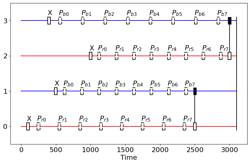
Fig. 8: An example circuit where non-aligned gate timings lead to difficulties in staggering DD for maximal crosstalk suppression.

Given any DD sequence drawn from $G=\{I,X\}$, we can easily calculate the effective time that any term $B^{i_{1},\dots,i_{4}}$ in the entangling system-bath Hamiltonian spends in forward evolution to first order in $\tau$ according to Eq. 13. In particular, we consider the error terms $Z_{1}Z_{2}I_{3}I_{4}$ and $I_{1}I_{2}Z_{3}Z_{4}$ that represent $ZZ$ crosstalk over both pairs of qubits connected by entangling gates. Additionally, we consider the error term $Z_{1}Z_{2}Z_{3}Z_{4}$ representing correlated $ZZ$ crosstalk over the pairs, as well as single-qubit errors $Z_{i}I_{j\mid j\neq i}$. We consider the following sample of DD strategies:

1. $P_{r}=P_{b}=XXXXXXXX$

2. $P_{r}=P_{b}=XIXIXIXI$

3. $P_{r}=XIXIXIXI$, $P_{b}=IXIXIXIX$

4. $P_{r}=XXXIIXII$, $P_{b}=XXXXIXIX$

5. $P_{r}=XXIXIXII$, $P_{b}=XIXXXXIX$

	Peekskill (BV)			Mumbai (Grover v1)			Mumbai (Grover v2)			Kyiv (MRB)
	Min	Mean	Max	Min	Mean	Max	Min	Mean	Max	Min	Mean	Max
$T_{1}$ ($\mu$s)	139.66	321.63	516.35	57.32	113.65	174.98	21.17	141.42	343.44	26.89	266.88	489.88
$T_{2}$ ($\mu$s)	23.66	299.26	536.11	27.06	167.27	343.3	27.06	167.27	343.3	15.17	143.31	416.68
1QG Error (%)	0.01	0.02	0.05	0.01	0.03	0.19	0.01	0.03	0.1	0.01	0.08	4.81
2QG Error (%)	0.39	0.8	1.37	0.49	0.91	2.1	0.49	0.91	1.76	0.43	1.98	100
1QG Duration ($\mu$s)	0.04	0.04	0.04	0.04	0.04	0.04	0.04	0.04	0.04	0.05	0.05	0.05
2QG Duration ($\mu$s)	0.43	0.6	0.62	0.25	0.45	0.74	0.25	0.45	0.74	0.61	0.64	0.66
RO Error (%)	0.37	1.97	9.59	1.0	2.84	8.02	1.	2.84	8.02	0.08	1.85	22.94
RO Duration ($\mu$s)	0.86	0.86	0.86	3.58	3.58	3.58	3.58	3.58	3.58	1.24	1.24	1.24

Table 2: Device specifications for ibm_peekskill, ibmq_mumbai and ibm_kyiv at the time of experiment execution are shown. Grover v1 and v2 refer to the Cliffordized and non-Cliffordized runs respectively. 1QG, 2QG, and RO denote 1-qubit gate, two-qubit gate, and readout, respectively.

The net forward evolution time of the aforementioned $H_{B,abcd}$ terms are depicted in Table 1 relative to the total circuit time of 3100 units for all $H_{B,abcd}$ terms without the presence of DD. Although the known DD strategies in strategies 1, 2, and 3 perform reasonably well to reduce the total time over which each term contributes to $H_{B,abcd}$, the non-aligned gate timings in the circuit lead to decreasing the effective time for error evolution when specific $X$ pulses are replaced with identity pulses. In particular, we note that strategy 3, which is the naive extension of the staggering formalism to this multi-qubit circuit, performs relatively poorly when it comes to suppressing $Z_{2}Z_{3}$ crosstalk with 1150 units of effective forward time evolution, compared to 0 units in the aligned-pulse quantum memory case. We note that this is because the presence of non-aligned gate timings disrupts the staggering of pulses when DD is padded to idle gaps uniformly; for example, $P_{r7}$ and $P_{b7}$ on qubits 2 and 3 occur much closer to each other in time than in the ideal staggering case.

For consideration, we present strategy 4 and strategy 5, which behave much closer to staggered sequences for quantum memory in terms of robustness to crosstalk in this generalized setting where gate timings are not aligned. We claim that the presence and location of the identity gates that enforce staggering in these strategies are difficult to ascertain a priori given the timings of idle gaps in the target circuit, and such considerations become even more difficult as the circuit depth and number of qubits grows to an experimentally relevant scale. Furthermore, we note that strategy 5 has perfect cancellation of both uncorrelated $ZZ$ and correlated $ZZZZ$ crosstalk to first order; however, it sacrifices suppression of single-qubit error evolution to do so. One can envision two backends; one with a much worse $Z_{0}Z_{1}$ crosstalk error and one with a much worse single-qubit error. An empirical search method such as the one presented in this paper would easily discern that strategy 5 is the more appropriate one to apply on the former while strategy 4 is the more appropriate one to apply on the latter. However, this balance is much more difficult to strike without backend feedback.

Appendix E Hardware and software specifications

All experimental results in this work were obtained through Qiskit [66]. The code for MRB circuits and analysis was written in Qiskit Experiments [67]. To quickly iterate in the genetic algorithm training process, Qiskit Runtime [68] was used to interleave quantum training circuits and the classical learning algorithm to evaluate the strategies.

Experiments were run on IBM superconducting quantum processors: ibm_peekskill and ibmq_mumbai are 27-qubit Falcon r5.10 and r8 processors, respectively. ibm_kyiv is a 127-qubit Eagle r3 processor. The machine specifications for all three devices for the data reported in this work are shown in Table 2.

References

- Viola et al. [1999] L. Viola, E. Knill, and S. Lloyd, Dynamical decoupling of open quantum systems, Physical Review Letters 82, 2417 (1999).
- Viola and Lloyd [1998] L. Viola and S. Lloyd, Dynamical suppression of decoherence in two-state quantum systems, Phys. Rev. A 58, 2733 (1998).
- Vitali and Tombesi [1999] D. Vitali and P. Tombesi, Using parity kicks for decoherence control, Physical Review A 59, 4178 (1999).
- Zanardi [1999] P. Zanardi, Symmetrizing evolutions, Physics Letters A 258, 77 (1999).
- Pokharel et al. [2018] B. Pokharel, N. Anand, B. Fortman, and D. A. Lidar, Demonstration of fidelity improvement using dynamical decoupling with superconducting qubits, Physical Review Letters 121, 220502 (2018).
- Ezzell et al. [2022] N. Ezzell, B. Pokharel, L. Tewala, G. Quiroz, and D. A. Lidar, Dynamical decoupling for superconducting qubits: a performance survey (2022), https://arxiv.org/2207.03670.
- Biercuk et al. [2009] M. J. Biercuk, H. Uys, A. P. VanDevender, N. Shiga, W. M. Itano, and J. J. Bollinger, Experimental Uhrig dynamical decoupling using trapped ions, Phys. Rev. A 79, 062324 (2009).
- Wang et al. [2012] Z. Wang, G. de Lange, D. Ristè, R. Hanson, and V. V. Dobrovitski, Comparison of dynamical decoupling protocols for a nitrogen-vacancy center in diamond, Phys. Rev. B 85, 155204 (2012).
- Riste et al. [2010] D. Riste, V. Dobrovitski, and R. Hanson, Universal dynamical decoupling of a single solid-state spin from a spin bath, Science 330, 60 (2010).
- Farfurnik et al. [2016] D. Farfurnik, A. Jarmola, L. Pham, Z. Wang, V. Dobrovitski, R. Walsworth, D. Budker, and N. Bar-Gill, Improving the coherence properties of solid-state spin ensembles via optimized dynamical decoupling, in Quantum Optics, Vol. 9900 (SPIE, 2016) pp. 111–120.
- Du et al. [2009] J. Du, X. Rong, N. Zhao, Y. Wang, J. Yang, and R. B. Liu, Preserving electron spin coherence in solids by optimal dynamical decoupling, Nature 461, 1265 (2009).
- Shor [1995] P. W. Shor, Scheme for reducing decoherence in quantum computer memory, Phys. Rev. A 52, R2493 (1995).
- Steane [1996] A. M. Steane, Error correcting codes in quantum theory, Phys. Rev. Lett. 77, 793 (1996).
- Shor [1996] P. Shor, Fault-tolerant quantum computation, in Proceedings of 37th Conference on Foundations of Computer Science (1996) pp. 56–65.
- Preskill [2018] J. Preskill, Quantum Computing in the NISQ era and beyond, Quantum 2, 79 (2018).
- AI [2023] G. Q. AI, Suppressing quantum errors by scaling a surface code logical qubit, Nature 614, 676 (2023).
- Kim et al. [2023a] Y. Kim, C. J. Wood, T. J. Yoder, S. T. Merkel, J. M. Gambetta, K. Temme, and A. Kandala, Scalable error mitigation for noisy quantum circuits produces competitive expectation values, Nat. Phys. 19, 752 (2023a).
- Kim et al. [2023b] Y. Kim, A. Eddins, S. Anand, K. Wei, E. Van Den Berg, S. Rosenblatt, H. Nayfeh, Y. Wu, M. Zaletel, K. Temme, and A. Kandala, Evidence for the utility of quantum computing before fault tolerance, Nature 618, 500 (2023b).
- Günlük et al. [2021] O. Günlük, T. Itoko, N. Kanazawa, et al., Demonstration of quantum volume 64 on a superconducting quantum computing system, Quantum Science and Technology 6, 025020 (2021).
- Ng et al. [2011] H. K. Ng, D. A. Lidar, and J. Preskill, Combining dynamical decoupling with fault-tolerant quantum computation, Phys. Rev. A 84, 012305 (2011).
- Genov et al. [2017] G. T. Genov, D. Schraft, N. V. Vitanov, and T. Halfmann, Arbitrarily accurate pulse sequences for robust dynamical decoupling, Phys. Rev. Lett. 118, 133202 (2017).
- Viola and Knill [2009] L. Viola and E. Knill, Robust dynamical decoupling of quantum systems with bounded controls, Phys. Rev. Lett. 90, 037901 (2009).
- Singkanipa et al. [2024] P. Singkanipa, V. Kasatkin, Z. Zhou, G. Quiroz, and D. A. Lidar, Demonstration of algorithmic quantum speedup for an abelian hidden subgroup problem, arXiv preprint arXiv:2401.07934 (2024).
- Pokharel and Lidar [2022] B. Pokharel and D. Lidar, Better-than-classical grover search via quantum error detection and suppression (2022), arXiv:2211.04543 .
- Pokharel and Lidar [2023] B. Pokharel and D. A. Lidar, Demonstration of algorithmic quantum speedup, Phys. Rev. Lett. 130, 210602 (2023).
- Tripathi et al. [2022] V. Tripathi, H. Chen, M. Khezri, K. Yip, E. Levenson-Falk, and D. A. Lidar, Suppression of crosstalk in superconducting qubits using dynamical decoupling, Phys. Rev. Appl. 18, 024068 (2022).
- Quiroz et al. [2024] G. Quiroz, B. Pokharel, J. Boen, L. Tewala, V. Tripathi, D. Williams, L. Wu, P. Titum, K. Schultz, and D. Lidar, Dynamically generated decoherence-free subspaces and subsystems on superconducting qubits (2024), arXiv:2402.07278 .
- Krantz et al. [2019] P. Krantz, M. Kjaergaard, F. Yan, T. P. Orlando, S. Gustavsson, and W. D. Oliver, A quantum engineer’s guide to superconducting qubits, Applied physics reviews 6 (2019).
- Zhou et al. [2023] Z. Zhou, R. Sitler, Y. Oda, K. Schultz, and G. Quiroz, Quantum crosstalk robust quantum control, Phys. Rev. Lett. 131, 210802 (2023).
- Zhang et al. [2022] H. Zhang, B. Pokharel, E. Levenson-Falk, and D. Lidar, Predicting non-markovian superconducting-qubit dynamics from tomographic reconstruction, Physical Review Applied 17, 054018 (2022).
- Córcoles et al. [2019] A. D. Córcoles, A. Mezzacapo, J. M. Chow, and J. M. Gambetta, Error mitigation extends the computational reach of a noisy quantum processor, Nature 567, 491 (2019).
- Van Den Berg et al. [2023] E. Van Den Berg, Z. K. Minev, A. Kandala, and K. Temme, Probabilistic error cancellation with sparse pauli–lindblad models on noisy quantum processors, Nature Physics , 1 (2023).
- Temme et al. [2017] K. Temme, S. Bravyi, and J. M. Gambetta, Error mitigation for short-depth quantum circuits, Physical Review Letters 119, 180509 (2017).
- Nation et al. [2021] P. D. Nation, H. Kang, N. Sundaresan, and J. M. Gambetta, Scalable mitigation of measurement errors on quantum computers, PRX Quantum 2, 040326 (2021).
- Van Den Berg et al. [2022] E. Van Den Berg, Z. K. Minev, and K. Temme, Model-free readout-error mitigation for quantum expectation values, Physical Review A 105, 032620 (2022).
- Pokharel et al. [2024] B. Pokharel, S. Srinivasan, G. Quiroz, and B. Boots, Scalable measurement error mitigation via iterative bayesian unfolding, Physical Review Research 6, 013187 (2024).
- Zlokapa and Gheorghiu [2020] A. Zlokapa and A. Gheorghiu, A deep learning model for noise prediction on near-term quantum devices (2020), arXiv:2005.10811 .
- Carr and Purcell [1954] H. Y. Carr and E. M. Purcell, Effects of diffusion on free precession in nuclear magnetic resonance experiments, Phys. Rev. 94, 630 (1954).
- Meiboom and Gill [1958] S. Meiboom and D. Gill, Modified spin-echo method for measuring nuclear relaxation times, Review of scientific instruments 29, 688 (1958).
- Das et al. [2021] P. Das, S. Tannu, S. Dangwal, and M. Qureshi, Adapt: Mitigating idling errors in qubits via adaptive dynamical decoupling, in MICRO-54: 54th Annual IEEE/ACM International Symposium on Microarchitecture (2021) pp. 950–962.
- Ravi et al. [2022] G. K. Ravi, K. N. Smith, P. Gokhale, A. Mari, N. Earnest, A. Javadi-Abhari, and F. T. Chong, VAQEM: A Variational Approach to Quantum Error Mitigation, in 2022 IEEE International Symposium on High-Performance Computer Architecture (HPCA) (2022) pp. 288–303.
- Quiroz and Lidar [2013] G. Quiroz and D. A. Lidar, Optimized dynamical decoupling via genetic algorithms, Physical Review A 88, 052306 (2013).
- Wu and Lidar [2002] L. Wu and D. A. Lidar, Creating decoherence-free subspaces using strong and fast pulses, Phys. Rev. Lett. 88, 207902 (2002).
- Lidar [2014] D. A. Lidar, Review of decoherence-free subspaces, noiseless subsystems, and dynamical decoupling, in Quantum Information and Computation for Chemistry (John Wiley & Sons, Ltd, 2014) Chap. 11, pp. 295–354.
- Polak [2012] E. Polak, Optimization: algorithms and consistent approximations, Vol. 124 (Springer Science & Business Media, 2012).
- Egger et al. [2023] D. J. Egger, C. Capecci, B. Pokharel, P. K. Barkoutsos, L. E. Fischer, L. Guidoni, and I. Tavernelli, Pulse variational quantum eigensolver on cross-resonance-based hardware, Phys. Rev. Res. 5, 033159 (2023).
- Reeves and Rowe [2002] C. Reeves and J. E. Rowe, Genetic algorithms: principles and perspectives: a guide to GA theory, Vol. 20 (Springer Science & Business Media, 2002).
- Mitchell [1999] M. Mitchell, An Introduction to Genetic Algorithms (MIT Press, Cambridge, 1999).
- Chamberland et al. [2020] C. Chamberland, G. Zhu, T. J. Yoder, J. B. Hertzberg, and A. W. Cross, Topological and subsystem codes on low-degree graphs with flag qubits, Phys. Rev. X 10, 011022 (2020).
- Proctor et al. [2022a] T. Proctor, K. Rudinger, K. Young, E. Nielsen, and R. Blume-Kohout, Measuring the capabilities of quantum computers, Nature Physics 18, 75 (2022a).
- Aaronson and Gottesman [2004] S. Aaronson and D. Gottesman, Improved simulation of stabilizer circuits, Phys. Rev. A 70, 052328 (2004).
- Bernstein and Vazirani [1993] E. Bernstein and U. Vazirani, Quantum complexity theory, in Proceedings of the twenty-fifth annual ACM symposium on Theory of computing (1993) pp. 11–20.
- Lubinski et al. [2023] T. Lubinski, S. Johri, P. Varosy, J. Coleman, L. Zhao, J. Necaise, C. H. Baldwin, K. Mayer, and T. Proctor, Application-oriented performance benchmarks for quantum computing, IEEE Transactions on Quantum Engineering (2023).
- Fallek et al. [2016] S. Fallek, C. Herold, B. McMahon, K. Maller, K. Brown, and J. Amini, Transport implementation of the Bernstein–Vazirani algorithm with ion qubits, New Journal of Physics 18, 083030 (2016).
- Wright et al. [2019] K. Wright, K. M. Beck, S. Debnath, J. Amini, Y. Nam, N. Grzesiak, J. Chen, N. Pisenti, M. Chmielewski, C. Collins, et al., Benchmarking an 11-qubit quantum computer, Nature Communications 10, 5464 (2019).
- The Qiskit Research developers and contributors [2023] The Qiskit Research developers and contributors, Qiskit Research (2023).
- Mundada et al. [2023] P. S. Mundada, A. Barbosa, S. Maity, Y. Wang, T. Merkh, T. Stace, F. Nielson, A. R. Carvalho, M. Hush, M. J. Biercuk, et al., Experimental benchmarking of an automated deterministic error-suppression workflow for quantum algorithms, Physical Review Applied 20, 024034 (2023).
- Lidar and Brun [2013] D. A. Lidar and T. A. Brun, Quantum error correction (Cambridge university press, 2013).
- Grover [1997] L. K. Grover, Quantum mechanics helps in searching for a needle in a haystack, Phys. Rev. Lett. 79, 325 (1997).
- Proctor et al. [2022b] T. Proctor, S. Seritan, K. Rudinger, E. Nielsen, R. Blume-Kohout, and K. Young, Scalable randomized benchmarking of quantum computers using mirror circuits, Physical Review Letters 129, 150502 (2022b).
- Magesan et al. [2011] E. Magesan, J. M. Gambetta, and J. Emerson, Scalable and robust randomized benchmarking of quantum processes, Physical review letters 106, 180504 (2011).
- Magesan et al. [2012] E. Magesan, J. M. Gambetta, and J. Emerson, Characterizing quantum gates via randomized benchmarking, Physical Review A 85, 042311 (2012).
- Hines et al. [2023] J. Hines, M. Lu, R. K. Naik, A. Hashim, J. Ville, B. Mitchell, J. M. Kriekebaum, D. I. Santiago, S. Seritan, E. Nielsen, R. Blume-Kohout, K. Young, I. Siddiqi, B. Whaley, and T. Proctor, Demonstrating scalable randomized benchmarking of universal gate sets, Phys. Rev. X 13, 041030 (2023).
- McKay et al. [2023] D. C. McKay, I. Hincks, E. J. Pritchett, M. Carroll, L. C. Govia, and S. T. Merkel, Benchmarking quantum processor performance at scale, arXiv preprint arXiv:2311.05933 (2023).
- Amico et al. [2023] M. Amico, H. Zhang, P. Jurcevic, L. S. Bishop, P. Nation, A. Wack, and D. C. McKay, Defining standard strategies for quantum benchmarks (2023), arXiv:2303.02108.
- Qiskit Contributors [2023] Qiskit Contributors, Qiskit: An Open-source Framework for Quantum Computing (2023).
- Kanazawa et al. [2023] N. Kanazawa, D. J. Egger, Y. Ben-Haim, H. Zhang, W. E. Shanks, G. Aleksandrowicz, and C. J. Wood, Qiskit Experiments: A Python package to characterize and calibrate quantum computers, Journal of Open Source Software 8, 5329 (2023).
- Johnson [2022] B. Johnson, Qiskit runtime, a quantum-classical execution platform for cloud-accessible quantum computers, in APS March Meeting Abstracts, Vol. 2022 (2022) pp. T28–002.