Magnetic Weyl-Kondo semimetals induced by quantum fluctuations

Abstract

Kondo effect exemplifies the type of quantum fluctuations driven by strong correlations, and its cooperation with space group symmetries underlies the Weyl-Kondo semimetals. Because the Kondo effect of the $f$-electrons is believed to be suppressed in a magnetic environment, Weyl-Kondo semimetals have so far been confined to paramagnetic settings. Here we develop the theory of magnetic Weyl-Kondo semimetal. The key of the proposed mechanism is that the magnetic order is originated from the conduction $d$ electrons, such that the local moments can still fluctuate. We illustrate the extreme case where the magnetic space group symmetries prevent any magnetization on the sites with the $f$-orbitals. In this case, hourglass Weyl-Kondo nodal lines appear when the space group symmetry acts on the Kondo-driven low-energy excitations. We suggest a third-order nonlinear spontaneous Hall response as a means to diagnose this type of topological crossings. Based on the theoretical mechanism, we explore the interplay between correlations and symmetries in magnetic square-net materials, leading to several candidate materials with a variety of nonlinear Hall responses. Our findings pave the way for future experimental exploration and theoretical investigations in this new and promising materials class as a part of an overarching effort to understand and harness the interplay between strong correlations and topology.

Introduction.— Strong correlations drive a variety of quantum phases [1, 2]. Weyl-Kondo semimetals (WKSMs) [3, 4] represent a fascinating intersection of the strong correlation physics with gapless electronic topology [5]. This interplay leads to a rich platform of emergent phenomena and exotic physical properties.

Weyl semimetals in noninteracting systems have emerged as an important class of semimetallic systems characterized by the topology of Weyl nodes, either in paramagnetic [5, 6, 7, 8] or magnetic environments [9, 10]. These nodes act as sources or sinks of Berry curvature, giving rise to intriguing phenomena such as chiral anomaly and Fermi arc surface states. In realizing Weyl semimetals, lattice symmetries play an important role as indicators of topology [5, 11]. On the other hand, Kondo physics describes the screening of localized magnetic moments by conduction electrons, leading to the formation of composite heavy fermions [12, 13].

In paragmagnetic WKSMs, these two paradigms coalesce to produce a novel class of materials with distinct physical properties. The cooperation between strong electron correlations and space group symmetry constraints can induce the Weyl nodes in the heavy fermion states, as revealed by recent non-perturbative studies [14, 3, 15, 16, 17]. Such novel phases have been explored in experiments in the material $\rm Ce_{3}Bi_{4}Pd_{3}$, based on measurements of specific heat and spontaneous Hall effect [4, 18, 19]. Potential materials candidates of WKSMs have been proposed thorough database-mining based on both space group symmetries and the reported physical properties [14].

Heavy fermion systems are often on the verge of magnetic order and, indeed, their interplay with magnetism is a prominent feature of the field. Thus, the lack of understanding for magnetic topological semimetals in heavy fermion systems represents a glaring hole in the field. To make progress, it is necessary to understand how the Kondo effect can operate in a magnetic environment given that a long-range order of the local moments is expected to inhibit their capacity for producing quantum fluctuations, and how the mechanism inter-plays with what drives topological crossings.

In this work, we confront this challenge and develop the theory of magnetic Weyl-Kondo semimetal (MWKSM). While a magnetic order breaks time-reversal symmetry, a suitable combination of the time-reversal symmetry and spatial symmetries can be preserved. Such symmetries are described by the magnetic space groups (MSGs), which have been classified and tabulated [20]. Here we demonstrate the development of MWKSM from the quantum fluctuations of the local moments when the MSGs describe a magnetic order that is driven by the conduction $d$ electrons. Our model calculations give rise to Kondo-driven magnetic hourglass Weyl nodal lines. To be definite, we focus on the MWKSMs in the square-net category given the large materials base in this category for topological semimetals [21, 22, 23, 24]. Since Weyl points and hourglass Weyl nodal lines are sources of Berry curvature, we find that the nonlinear anomalous Hall effect [25, 26, 27] provides telltale signatures of the symmetries that are broken in the MSGs for MWKSMs.

Specifically, we study the Anderson/Kondo lattice model in several square-net MSGs, with a particular focus on MSG no. 129.415 to illustrate our case. In the presence of the $d$-electron-driven magnetic order, the $f$-electron local moment can still fluctuate because the space group symmetry prevents the magnetization on the sites with the $f$-orbitals. In turn, we show how, through the space-group symmetry constraints [28], Kondo-driven hourglass Weyl nodal lines develop and induce a 3rd-order nonlinear Hall response. We also report related results for several other MSGs. Armed with the theoretical results, we outline a materials design procedure for MWKSMs with symmetry-constrained topological crossings, and identify a set of candidate materials with strong correlations that are expected to feature the symmetry enforced non-linear Hall responses.

MWKSM in a magnetic square net model—

Figure 1: Unit cell of a model material in MSG no. 129.415 ($P4^{\prime}/nmm^{\prime}$). The AFM ordering on the $\rm TM$ atoms are illustrated by arrows. The correlated $f$-electrons come from the $\rm Ce$ atoms.

We present one example of MWKSM in square-net materials, with MSG no. 129.415 ($P4^{\prime}/nmm^{\prime}$). We assume there are $\rm Ce$ and transition metal ($\rm TM$) atoms. The $\rm Ce$ atoms are at the $2a$ Wyckoff position and the $\rm TM$ atoms are at the $4d$ Wyckoff position. The magnetic moments on $\rm TM$ atoms are ordered, as shown in Fig. 1, due to interactions among the $d$ electrons. The four-fold rotation centers are at the $\rm Ce$ positions. The $C_{4}{\cal T}$ symmetry ensures that no magnetic ordering can appear at the $2a$ Wyckoff position. The $f$ electrons are from the $\rm Ce$ atoms. The symmetries operations and their representations are discussed in Supplemental Material (SM) [29].

To expound further on the advantages of this set up, we note on the following. The $\rm Ce$ sites are always nonmagnetic as a consequence of its site symmetry group. Therefore, there is no induced magnetic ordering to weaken the heavy fermion phase. Second, the $\rm TM$ sites can host magnetic order. The electrons from the $\rm TM$ atoms provide a magnetic environment for the electrons from $\rm Ce$ atoms, resulting in momentum dependent spin-splittings.

We construct a model with orbitals at the $\rm Ce$ atoms. The orbitals from other atoms provide a crystal potential that constraint the hoppings of the $\rm Ce$-bound orbitals. We consider one of the conduction-electron orbitals from the $\rm Ce$ atom that, as standard, is taken as non-interacting. The Hamiltonian of the itinerant electrons is

$$H_{c}= \sum_{k}\Psi_{k}^{\dagger}\left(h({\mathbf{k}})-\mu\right)\Psi_{k}$$ (1)

$$h({\mathbf{k}})= t\cos(\frac{k_{x}}{2})\cos(\frac{k_{y}}{2})\sigma_{0}\tau_{x}+t_{z}\sin(k_{z})\cos(\frac{k_{x}}{2})\cos(\frac{k_{y}}{2})\sigma_{0}\tau_{y}$$

$$+t_{SOC}\big{(}\sin(k_{x})\sigma_{y}+\sin(k_{y})\sigma_{x}\big{)}\tau_{z}$$

$$+t_{SOC}^{\prime}\sin(\frac{k_{x}}{2})\sin(\frac{k_{y}}{2})\sigma_{z}\tau_{x}$$

$$+t_{SOC}^{\prime\prime}\left(\cos(\frac{k_{x}}{2})\sin(\frac{k_{y}}{2})\sigma_{x}+\sin(\frac{k_{x}}{2})\cos(\frac{k_{y}}{2})\sigma_{y}\right)\tau_{y}\,,$$ (2)

where $\mu$ is chemical potential, $\Psi=(c_{A\uparrow},c_{A\downarrow},c_{B\uparrow},c_{B\downarrow})$ is the annihilation operator of itinerant electrons at the two $\rm Ce$ sublattice sites $A$ and $B$ with the two spin degrees, $\sigma$ and $\tau$ are the Pauli matrices that describe the spin and sublattice degrees respectively. The first and second lines of $h({\mathbf{k}})$ preserve $P4/nmm1^{\prime}$ while the third and fourth lines preserve $P4^{\prime}/nmm^{\prime}$, which are responsible for the spin splitting.

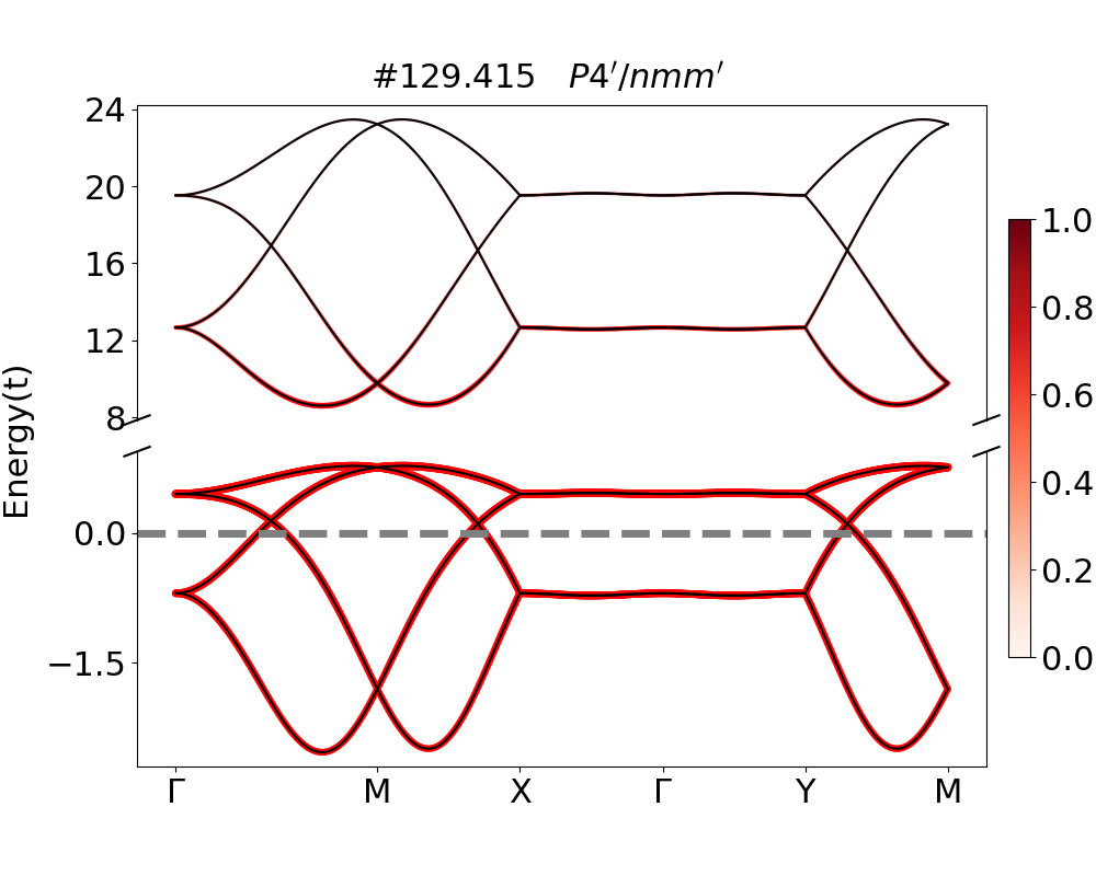
Figure 2: Kondo-driven Weyl hourglass nodal line excitations. The result is derived from a saddle-point solution to the model Eq. (3), and is shown as the energy vs. the wavevector $\bf{\rm k}$ along a high-symmetry direction. Red color indicates the weight of the $f$ electrons in the states.

The $f$ electrons in the $\rm Ce$ atoms are at the energy level $\epsilon_{f}$ and have an on-site Hubbard interaction $U$. We consider the large $U$ limit. Here the system is effectively described by a slave-boson representation [13]. This model is solved at the saddle-point level, which formally develops in a large-$N$ limit [13]. The effective Hamiltonian is given as follows:

$$\begin{split}H=H_{c}+\sum_{j,\alpha,m}\epsilon_{f}f_{j\alpha m}^{\dagger}f_{j\alpha m}+rV\left[c_{j\alpha m}^{\dagger}f_{j\alpha m}+\text{ h.c. }\right]\\ +\lambda\sum_{j}(n_{f,j}+r^{2}-Q)\,.\end{split}$$ (3)

Here, $H_{c}$ is the non-interacting Hamiltonian for the $c$ electrons defined in Eq. (1). In addition, $r=\langle b_{j}\rangle$ is the condensed slave boson field $b_{j}$, while $c_{j\alpha m}$ and $f_{j\alpha m}$ represent the itinerant and heavy electrons at site $j$, orbital $\alpha$, spin $m$ while $n_{f,j}=\sum_{\alpha m}f^{\dagger}_{j\alpha m}f_{j\alpha m}$ represents the number of $f$ electrons at site $j$. The filling is constraint to $Q=1$. The $\lambda$ term comes from the Lagrange multiplier of the local filling constraint $n_{f,j}+b^{\dagger}b=Q$. The self-consistent equations read as follows:

$$\langle n_{f,j}\rangle+r^{2} =Q$$ (4)

$$V\sum_{\alpha,m}\langle c_{j\alpha m}^{\dagger}f_{j\alpha m}\rangle =-2\lambda r$$ (5)

where $\langle\cdot\rangle$ means averaging over all sites. We iteratively solve the self-consistent equations to find the physical values of $\lambda$ and $r$. During this calculation, we set $\mu=-r^{2}V^{2}/\lambda$ to maintain the physical filling factor. Without loss of generality, we consider the case with the parameters $t=1$ (defined as the energy unit), $t_{z}=0.5$, $t_{SOC}=0.5$, $t_{SOC}^{\prime}=2$, $t_{SOC}^{\prime\prime}=1$, $V=10$, $\epsilon_{d}=-5$. The self-consistent calculation yields $r^{2}=0.327$, $\lambda=1.76$ and $\mu=-18.6$.

Fig. 2 shows the energy dispersion at $k_{z}=0$. The top four dispersive wide bands mainly describe the itinerant electrons, with symmetry-enforced crossings that occur far away from the Fermi energy, as it generically should be. On the other hand, the bottom four narrow bands are Kondo-driven, capturing the $f$ electrons that develop from the Kondo effect. Because these states are emergent, driven by the stron interactions, they lie at low energies and, as such, they are bound to the Fermi energy. These emergent states are subject to symmetry constraints. The result is the formation of hourglass Weyl Kondo nodal lines.

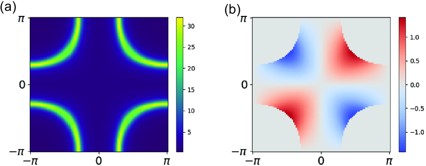
Figure 3: (a) Spectral function $A(k,\omega=0.1)$ shows the Kondo-driven hourglass Weyl nodal lines of the $f$-electron states of Fig. 2, where the hourglass Weyl nodal lines reside. (b) Berry curvature of the states below Fermi energy, showing a quadrupole-shaped distribution.

The hourglass Weyl nodal lines and Berry curvature of states below the Fermi energy are shown in Fig. 3. The Berry curvature distribution has hot spot around these nodal lines. This distribution is quadrupole-shaped that signals the 3rd-order nonlinear Hall response driven by Berry curvature quadrupoles. The 3rd-order Hall response is defined by $j^{\mu}=\sigma^{\mu;\alpha\beta\gamma}E_{\alpha}E_{\beta}E_{\gamma}$. It has $1\omega$ and $3\omega$ responses where $\omega$ is the frequency of the electric field. The 3rd-order response conductivity captures the second order derivate of the Berry curvature [25]. The nonzero Berry curvature quadrupole is $Q_{xy;z}$ which leads to an in-plane current $j^{x}\propto E_{x}E_{y}^{2}$.

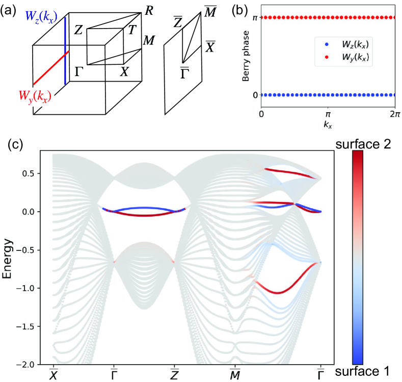
Figure 4: (a) Bulk and surface Brillouin zones. The directions of Wilson loops $W_{z}(k_{x})$ and $W_{y}(k_{x})$ are depicted. (b) Wilson loops $W_{z}(k_{x})$ at $k_{y}=\pi/2$ and $W_{y}(k_{x})$ at $k_{z}\neq 0,\pi$. The nonzero Berry phase $W_{y}(k_{x})=\pi$ indicates polarization $p_{x}=p_{y}=1/2$ at the $k_{z}$ planes with $k_{z}\neq 0,\pi$. (c) Surface states with a slab geometry. The colored states are localized at the two boundaries. The presence of the localized surface states along $\overline{\Gamma}\overline{Z}$ are results of the quantized polarizations.

The lower two bands below the Fermi energy are gapped except at the hourglass Weyl nodal lines. This allows us to calculate the Wilson loop of these two bands. We compute the Wilson loop along $k_{x}$ direction for $k_{x}\in[0,2\pi]$. The results, shown in Fig. 3(a), reveals a $\pi$ Berry phase for the two bands. This Berry phase indicates the quantized polarization $p_{x}=p_{y}=1/2\mod 1$ in unit of $|e|a$ where $e$ is the electron charge and $a$ is the lattice constant. As a consequence of the Berry phase, there are mid gap surface states at the Fermi energy that are localized on the boundaries of finite systems. These states are shown in Fig. 4(b) with red and blue colors representing the two boundaries.

The hourglass Weyl nodal lines are consequences of compatibility conditions in momentum space. For example, in MSG no. 129.415 the compatibility condition forces the irreducible representations (irreps) connectivity: $\overline{\Gamma}_{5}(2)\rightarrow\overline{D}_{3}(1)\oplus\overline{D}_{4}(1)$, $\overline{\Gamma}_{6}(2)\rightarrow\overline{D}_{3}(1)\oplus\overline{D}_{4}(1)$ and $\overline{M}_{3}(2)\rightarrow\overline{D}_{4}(1)\oplus\overline{D}_{4}(1)$, $\overline{M}_{4}(2)\rightarrow\overline{D}_{3}(1)\oplus\overline{D}_{3}(1)$, where $D=(u,v,0)$, $\Gamma=(0,0,0)$, $M=(\pi,\pi,0)$. Therefore, there are symmetry enforced hourglass Weyl nodal lines in the $k_{z}=0$ plane [20].

This illustrating example shows that MWKSMs can have symmetry enforced crossings and nonlinear Hall effects. In the SM [29] we show more examples of MSGs in the space group no. 129 family. With these solutions in place, we turn to the general discussion about how to identify these physical properties from symmetry considerations.

Magnetic space groups of square-net systems and physical properties.— Our calculations described above illustrate an important point for magnetic heavy fermion systems. The emergent composite heavy fermions, driven by the Kondo effect, are bound to the Fermi energy even in a magnetic environment. We will thus utilize symmetry considerations to search for suitable materials to realize the MWKSMs. Of our interest are a number of physical properties, which are all constrained by symmetries. These include (1) the symmetry enforced crossings; (2) symmetry constraints on the magnetic ordering; and (3) symmetry constraints on the nonlinear Hall response. These are described in some detail in the SM [29].

To set the stage for the identification of candidate materials, we restrict to square-net materials, which are in MSGs that have square (tetragonal) crystal lattices without any one-fold Wyckoff position. The typical square-net materials are in SGs no. 129 and no. 139 [22]. However, the actual MSGs that have square-net lattices are not limited to these groups [22, 23, 21]. As an example, we summarize 129 family of MSGs in Table 1. Specifically, MSG no. 129.417 is compatible with ferromagnetic (FM) ordering while all MSGs in this family, except no. 129.412, are compatible with certain AFM ordering. MSGs no. 129.411, 129.414, 129.415 have 3rd-order Hall response as the leading order.

MSG #	BNS	FM	AFM	Hall response	Crossing
129.411	$P4/nmm$		✓	3rd-order	Dirac
129.412	$P4/nmm1^{\prime}$				Dirac
129.413	$P4/n^{\prime}mm$		✓		Dirac
129.414	$P4^{\prime}/nm^{\prime}m$		✓	3rd-order	Dirac
129.415	$P4^{\prime}/nmm^{\prime}$		✓	3rd-order	HWNL
129.416	$P4^{\prime}/n^{\prime}m^{\prime}m$		✓
129.417	$P4/nm^{\prime}m^{\prime}$	✓	✓	1st-order
129.418	$P4^{\prime}/n^{\prime}mm^{\prime}$		✓		Dirac
129.419	$P4/n^{\prime}m^{\prime}m^{\prime}$		✓
129.420	$P_{c}4/nmm$		✓		Dirac
129.421	$P_{C}4/nmm$		✓		Dirac
129.422	$P_{I}4/nmm$		✓		Dirac

Table 1: MSGs of space group no. 129 family. We use BNS setting to denote the MSGs [20]. The magnetic orderings compatible with each MSG are marked with $\checkmark$. Blank means the magnetic ordering is not compatible with the group. The leading order Hall response of each group is listed. Blank means no Hall response of any order is permitted. The crossing types for bands from $s$-orbitals at $2a$ Wyckoff positions are listed. Blank means no symmetry-enforced Dirac or hourglass Weyl nodal line (HWNL) exists in the group.

In Table. 1 we also list the crossings other than Weyl points and gapped phases. Weyl points can appear in all of these groups except MSG no. 129.412, 129.413, 129.416 and 129.418-129.422 where ${\cal PT}T_{\mathbf{r}}$ symmetry is present ($\cal P$ is inversion, $\cal T$ is time-reversal symmetry, and $T_{\mathbf{r}}$ can be any fractional translation). Symmetry enforced Dirac points and hourglass Weyl nodal lines can appear in some of these groups. As is also seen, the Hall responses of orders one, two, three as leading order can be found for different MSGs.

We also list MSG families 125 and 31 for comparison in the SM [29].

Material candidates.—

Materials	MSG #	BNS	Hall	Crossing
$\rm CeMn_{2}Ge_{4}O_{12}$ [30]	125.367	$P4^{\prime}/nbm^{\prime}$	3rd-order	HWNL
$\rm Ce_{4}Ge_{3}$ [31]	122.333	$I\bar{4}2d$	2nd-order
$\rm Ce_{4}Sb_{3}$ [32]	122.336	$I\bar{4}^{\prime}2d^{\prime}$	2nd-order	Dirac
$\rm Ce_{3}NIn$ [33]	117.305	$P_{C}\bar{4}b2$	2nd-order	HWNL
$\rm CeNiAsO$ [34]	4.10	$P_{a}2_{1}$	2nd-order	HWNL
$\rm CeAuSb_{2}$ [35, 36]	39.201	$A_{b}Bm2$	2nd-order
$\rm CeCuGa_{3}$ [37]	44.230	$Imm21^{\prime}$	2nd-order
$\rm CeCu_{2}Ge_{2}$ [38]	44.230	$Imm21^{\prime}$	2nd-order

Table 2: Examples of $\rm Ce$ based materials with non-vanishing nonlinear Hall responses. The symmetry enforced crossings are listed. HWNL stands for hourglass Weyl nodal lines.

In our quest for MWKSM materials, we employ a systematic approach focused on identifying square net materials that exhibit a magnetic order, strong correlation effects, and semimetallic behavior. The following outlines our strategy for material selection:

1. Magnetic ordering: we search for materials that have either FM or AFM order. Each magnetic ordering corresponds to a MSG. The magnetic ordering is preferable if they are coming from $d$ electrons; this is indicated by a sufficiently high Curie temperature or Néel temperature. We are in particular interested in the MSGs that have nonlinear Hall effects as the leading order responses.

2. Strong electron correlation: The Kondo physics captures the quantum fluctuations associated with the underlying strong correlations. We filter the materials based on specific heat measurements. A large Sommerfeld coefficient $\gamma$, determined from $C_{p}/T$ at low temperatures (where $C_{p}$ is the specific heat), serves as a proxy for enhanced quantum fluctuations driven by electronic correlations.

3. Semimetallicity: We seek materials with semimetallic behaviors, as evidenced by a small band gap or a samll carrier concentration. Such materials are potential Kondo semimetals.

We show the database-mined information in SM [29]. Our material search leads to candidates that have non-linear Hall responses. We list those materials in Table 5, showing the MSGs, leading order Hall responses and the types of symmetry enforced crossings. We note in particular on two candidate materials. $\rm CeMn_{2}Ge_{4}O_{12}$ has MSG no. 125.367 which is very similar to MSG no.129.415 as we discuss in the SM [29]. The AFM order must come from $\rm Mn$ because $\rm Ce$ Wyckoff position is nonmagnetic due to symmetries. This material is a prime candidate to experimentally confirm it is semimetalic and strongly interacting. $\rm CeNiAsO$ has $d$ electron AFM order with Néel temperature $130$K and is strongly interacting. Measurement of nonlinear Hall responses will be illuminating.

Discussion.— We remark on several important points. Firstly, in order to perform calculations for a substantial number of MSGs, we have treated the Anderson lattice models at a saddle-point level. Going beyond this level, the quasiparticles remain robust but will acquire damping. The topological crossings we have shown will be robust based on the symmetry constraints of Green’s function eigenvectors [17].

Secondly, we have emphasized the signatures in terms of the nonlinear spontaneous Hall effect, because this quantity has played a key role in the identification of the WKSMs in the paramagnetic settings, as shown in experiments [18] and considered theoretically [15]. Still, other experimental signatures can be considered. For example, the hourglass Weyl Kondo nodal lines are expected to show signs both in the temperature dependence of the specific heat [3, 4] and in the STM spectrum [14].

Finally, our mateirials search has identified a number of Ce-based square-net heavy-fermion materials in which the electronic topology is manifested in either second-order or third-order nonlinear anomalous Hall effects. None of these properties have ever been considered before for heavy fermion systems or, to our knowledge, any other magnetic metals showing extreme strong correlations. We hope that our proposal will motivate such experiments in these broad classes of quantum materials.

To summarize, we have developed the theory of magnetic Weyl-Kondo semimetal. We formulate the theory in terms of a magnetic order that originates from the conduction ($d$) electrons, such that the $f$-electron local moments are still able to fluctuate and strong correlations can still induce amplified quantum fluctuations in spite of the static magnetic order. We have illustrated how the symmetries of the magnetic space groups play an essential role in several regards. These include enabling the $f$-electron quantum fluctuations in magnetic settings, constraining topological crossings of the Kondo-driven low-energy excitations, as well as giving rise to nonlinear anomalous Hall effects. Our results allow us to advance a design procedure for the magnetic Weyl-Kondo semimetals. The candidate materials we have proposed allow for experimental measurements that have never been attempted before in magnetic metals with extreme strong correlations. As such, our work not only advances the enormously challenging field of strongly correlated topological matter but also opens new directions for the investigations on the venerable interplay between strong quantum fluctuations and electronic orders through the new lenses that are provided by the perspective of correlated gapless topology.

Acknowledgement.— We thank Jennifer Cano, Maia Vergniory and, especially, Silke Paschen, for useful discussions. Work at Rice has primarily been supported by the Air Force Office of Scientific Research under Grant No. FA9550-21-1-0356 (conceptualization and model construction, Y.F.) by the National Science Foundation under Grant No. DMR-2220603 (model calculations, Y.F. and L.C.), by the Robert A. Welch Foundation Grant No. C-1411 and the Vannevar Bush Faculty Fellowship ONR-VB N00014-23-1-2870 (Q.S.). The majority of the computational calculations have been performed on the Shared University Grid at Rice funded by NSF under Grant EIA-0216467, a partnership between Rice University, Sun Microsystems, and Sigma Solutions, Inc., the Big-Data Private-Cloud Research Cyberinfrastructure MRI-award funded by NSF under Grant No. CNS-1338099, and the Extreme Science and Engineering Discovery Environment (XSEDE) by NSF under Grant No. DMR170109. All authors acknowledge the hospitality of the Kavli Institute for Theoretical Physics, UCSB, supported in part by the National Science Foundation under Grant No. NSF PHY-1748958, during the program “A Quantum Universe in a Crystal: Symmetry and Topology across the Correlation Spectrum.” Q.S. also acknowledges the hospitality of the Aspen Center for Physics, which is supported by the National Science Foundation under Grant No. PHY-2210452.

Magnetic Weyl-Kondo semimetals induced by quantum fluctuations
SUPPLEMENTAL MATERIAL

Appendix A MSGs – Symmetry considerations

The symmetry groups compatible with magnetic orderings are described by MSGs. Due to the existence of magnetic moment, time-reversal symmetry ${\cal T}$ is broken. However, some of the products of spatial symmetries and ${\cal T}$ can be preserved. There are in total 1651 MSGs including 230 SGs without ${\cal T}$, 230 grey groups (SGs with ${\cal T}$), 674 type III MSGs (SGs with spatial-time-reversal symmetry except for translation-time-reversal symmetry) and 517 type IV MSGs (SGs with translation-time-reversal symmetry).

The magnetic ordering is determined by both the MSG and the site-symmetry group of the magnetic moment. The latter constrain the orientation of magnetic moment on each site while the former constrain the relation of magnetic moments on different sites. Mathematically speaking, given a MSG $\cal G$ and a position $\mathbf{q}$ with its site symmetry group $G_{\mathbf{q}}$, we have the coset-decomposition ${\cal G}=\bigcup_{\alpha}g_{\alpha}G_{\mathbf{q}}$ where $g_{\alpha}$ can be either unitary or anti-unitary symmetries. For a compatible magnetic ordering, the magnetic momentum $\mathbf{m}$ of a certain orientation located at $\mathbf{q}$ is invariant under $G_{\mathbf{q}}$, forming an irreducible representation of $G_{\mathbf{q}}$. Then unitary $g_{\alpha}=\{R_{g_{\alpha}}|{\mathbf{t}}_{g_{\alpha}}\}$ maps $\mathbf{q},\mathbf{m}\mapsto R_{g_{\alpha}}\mathbf{q}+{\mathbf{t}}_{g_{\alpha}},R(g_{\alpha})\mathbf{m}$; anti-unitary $g_{\alpha}=\{R_{g_{\alpha}}|{\mathbf{t}}_{g_{\alpha}}\}{\cal T}$ maps it to $R_{g_{\alpha}}\mathbf{q}+{\mathbf{t}}_{g_{\alpha}},-R(g_{\alpha})\mathbf{m}$. Therefore, the magnetic ordering is uniquely determined by $\cal G$ and $G_{\mathbf{q}}$.

The nonlinear Hall responses result from Berry curvature multipoles. The $n$-th order nonlinear Hall response is $j^{\mu}=\sigma^{\mu;\alpha_{1}\dots\alpha_{n}}E_{\alpha_{1}}\dots E_{\alpha_{n}}$. This nonlinear Hall conductivity is determined by the $n$-th moment of Berry curvature $Q^{(n)}_{\beta_{1}\dots\beta_{n-1};\delta}=\sum_{n}\int_{\text{BZ}}f_{n}^{(0)}\partial_{\beta_{1}}\dots\partial_{\beta_{n}-1}\Omega_{n}^{\delta}$, where $f_{n}^{(0)}$ is the Fermi-Dirac distribution of the $n$-th band and $\Omega_{n}$ is the Berry curvature of that band. The Berry curvature multipoles are determined by the magnetic point group of the MSG $\cal G$, which is the quotient group of MSG mod the lattice translation group, i.e. ${\cal G}/{\mathbb{T}}$ [20]. Whether Berry curvature multipoles of each orders vanish or not can be determined by checking the transformation of Berry curvature multipoles under the magnetic point group [26]. If under a symmetry $g\in{\cal G}$, $gQ^{(n)}_{\beta_{1}\dots\beta_{n-1};\delta}\mapsto-Q^{(n)}_{\beta_{1}\dots\beta_{n-1};\delta}$, then $Q^{(n)}_{\beta_{1}\dots\beta_{n-1};\delta}=0$. If all the components of order $n$ vanish, then there is no $n$-th order Hall response in this MSG. From this analysis, the leading order Hall responses of MSGs can be determined.

MSGs can be viewed as symmetry breaking of the grey groups, which are the space groups with time-reversal symmetry. The crystal potentials that break the grey group symmetries lead to different spin-splittings in the band structure according to the corresponding MSGs. The spin-splittings can create various crossing types especially in these nonsymmorphic groups.

In the grey group MSG no. 129.412, the symmetry enforced Dirac point is pinned at high symmetry momenta by the interplay between time-reversal, mirror and glide symmetries which only allow four-dimensional irreps. For other MSGs with symmetry enforced Dirac points, they are protected by the unbroken symmetries at those momenta. The detailed reasoning can be made by checking the Frobenius-Schur index of the irreps of the maximal unitary group of the little co-group [20, 10].

Appendix B Details of the tight binding model in MSG no. 129.415

The model we introduce in the main text is a three-dimensional model. In the main text, we only show the band structure of $k_{z}=0$ plane. The full Brillouin zone band structure is given here in Fig. 5. In this model, $k_{z}=0$ and $k_{z}=\pi$ has the same features: they both have hourglass Weyl nodal lines surrounding the $(\pi,\pi)$ point; the Berry curvature distributions are both quadrupole shaped with the same signs. In the planes of $k_{z}\neq 0,\pi$, there are no hourglass Weyl nodal lines, as the bands along $A\Gamma$ line show. This is because mirror symmetry $m_{(001)}$ is protecting the crossings at $k_{z}=0,\pi$. There are two-fold degenerate bands along $\Gamma X$, $\Gamma Z$, $ZT$, $XR$, $MA$ due to the interplay of mirror and glide symmetries.

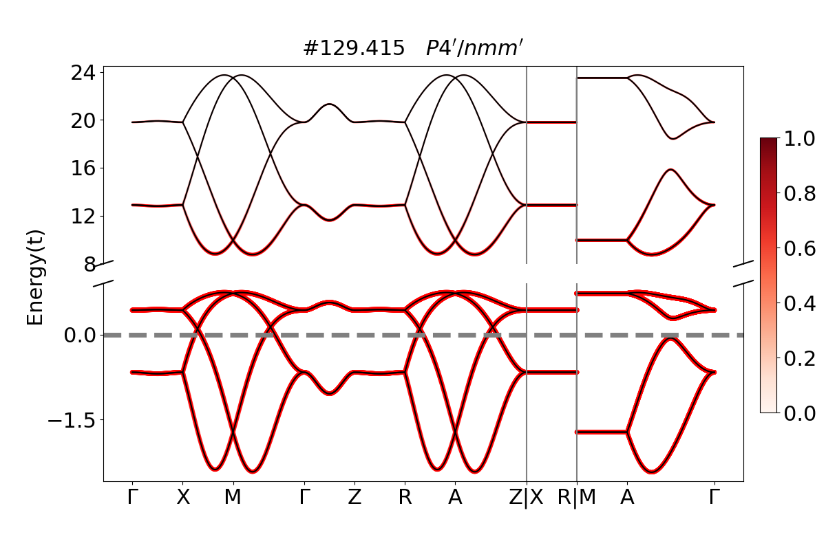
Figure 5: Energy dispersion of the Kondo-driven states along high symmetry lines in the three-dimensional Brillouin zone.

The hourglass Weyl nodal line in the $k_{z}=\pi/2$ plane is shown in Fig. 6(a). The anti-crossings at $k_{z}\neq 0,\pi$ where the gap is small are the hot spots of Berry curvature. The Berry curvature distribution at $k_{z}=\pi/2$ plane is shown in Fig. 6(b).

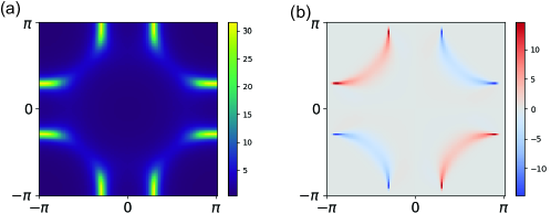
Figure 6: (a) hourglass Weyl nodal lines and (b) Berry curvature distribution at $k_{z}=\pi/2$.

The magnetic ordering in the TM atoms are the sources of the spin-splitting terms $t_{SOC}^{\prime}$ and $t_{SOC}^{\prime\prime}$. Here we study the dependence of $r=\langle b\rangle$ with this spin-splitting strength scaled by $t_{SOC}^{\prime}$. In this calculation, we choose $t_{SOC}^{\prime\prime}=2t_{SOC}^{\prime}$, and fix the energy of the itinerant electron band bottom. We show that $r$ decreases with the increase of $t_{SOC}^{\prime}$ in Fig. 7. Notice, the magnitude of $t_{SOC}^{\prime}$ does represent the magnetic moment. In realistic systems, the effective value of $t_{SOC}^{\prime}$ must be within a range $[0,t_{cutoff}]$. The values depend on the microscopic model of the full system.

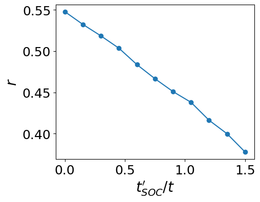
Figure 7: $r$ dependence on the spin-splitting strength.

Appendix C Examples in MSG 129 family and MSG 125.367

In this section we first present additional examples in the MSG 129 family. The symmetries of these groups are a subset of the grey group $P4/nmm1^{\prime}$. For this grey group the generators are time-reversal symmetry $\cal T$, four-fold rotation symmetry $C_{4}$ about the $(\frac{1}{4},\frac{1}{4},z)$ axis, inversion symmetry $\cal P$ centered at the origin, and two-fold screw symmetry $\{C_{2x}|\frac{1}{2}00\}$. In the basis of $s$-orbitals with spin-orbit coupling at $2a$ Wyckoff position, they are represented by

$${\cal T} =-i\sigma_{y}\tau_{0}{\hat{\cal K}}$$ (6)

$${\cal P} =\sigma_{0}\tau_{x}$$ (7)

$${C_{4}} =\frac{\sigma_{0}-\sigma_{z}}{\sqrt{2}}\tau_{0}$$ (8)

$${C_{2x}} =-i\sigma_{x}\tau_{x}$$ (9)

where ${\hat{\cal K}}$ is the complex conjugation operator, $\sigma$ and $\tau$ are Pauli matrices that describe spin degrees and sublattice degrees, respectively. The MSGs we study in this section include no. 129.411 ($P4/nmm$), no. 129.412 ($P4/nmm1^{\prime}$), no. 129.414 ($P4^{\prime}/nm^{\prime}m$) and no. 129.417 ($P4/nm^{\prime}m^{\prime}$). The compatible magnetic ordering and nonlinear Hall responses are listed in Table 1 in the main text. The itinerant electron Hamiltonian of these groups are of the form

$$H_{c}({\mathbf{k}}) =\sum_{k}\Psi_{k}^{\dagger}\left(h_{0}({\mathbf{k}})+h_{1}({\mathbf{k}})-\mu\right)\Psi_{k}$$ (10)

$$h_{0}({\mathbf{k}})= t\cos(\frac{k_{x}}{2})\cos(\frac{k_{y}}{2})\sigma_{0}\tau_{x}+t_{z}\sin(k_{z})\cos(\frac{k_{x}}{2})\cos(\frac{k_{y}}{2})\sigma_{0}\tau_{y}$$

$$+t_{SOC}\big{(}\sin(k_{x})\sigma_{y}+\sin(k_{y})\sigma_{x}\big{)}\tau_{z}$$ (11)

and $h_{1}({\mathbf{k}})$ contains the spin-orbit coupling terms that break $P4/nmm1^{\prime}$ into the desired MSGs. The band structures of these models are shown in Figs. 8, 9, 10 and 11. The different types of spin splittings can be seen from these plots. The spin splittings can be checked by studying the symmetries at those momenta. The types of symmetry enforced crossings agree with Table 1 in the main text.

The corresponding spin-orbit coupling terms $h_{1}({\mathbf{k}})$, with the aforementioned groups labeled by the MSGs in order, are as follows

$$h_{1}^{(129.411)}({\mathbf{k}}) =t_{SOC}^{\prime\prime}\left(\cos(\frac{k_{x}}{2})\sin(\frac{k_{y}}{2})\sigma_{x}-\sin(\frac{k_{x}}{2})\cos(\frac{k_{y}}{2})\sigma_{y}\right)\tau_{y}$$ (12)

$$h_{1}^{(129.412)}({\mathbf{k}}) =0$$ (13)

$$h_{1}^{(129.414)}({\mathbf{k}}) =+t_{SOC}^{\prime}\sin(\frac{k_{x}}{2})\sin(\frac{k_{y}}{2})\sigma_{z}\tau_{x}$$

$$+t_{SOC}^{\prime\prime}\left(\cos(\frac{k_{x}}{2})\sin(\frac{k_{y}}{2})\sigma_{x}+\sin(\frac{k_{x}}{2})\cos(\frac{k_{y}}{2})\sigma_{y}\right)\tau_{y}$$ (14)

$$h_{1}^{(129.417)}({\mathbf{k}}) =t_{SOC}^{\prime\prime}\left(\cos(\frac{k_{x}}{2})\sin(\frac{k_{y}}{2})\sigma_{x}+\sin(\frac{k_{x}}{2})\cos(\frac{k_{y}}{2})\sigma_{y}\right)\tau_{y}$$

$$+t_{SOC}^{\prime\prime\prime}\big{(}\cos(k_{x})+\cos(k_{y})\big{)}\sigma_{z}\tau_{0}$$ (15)

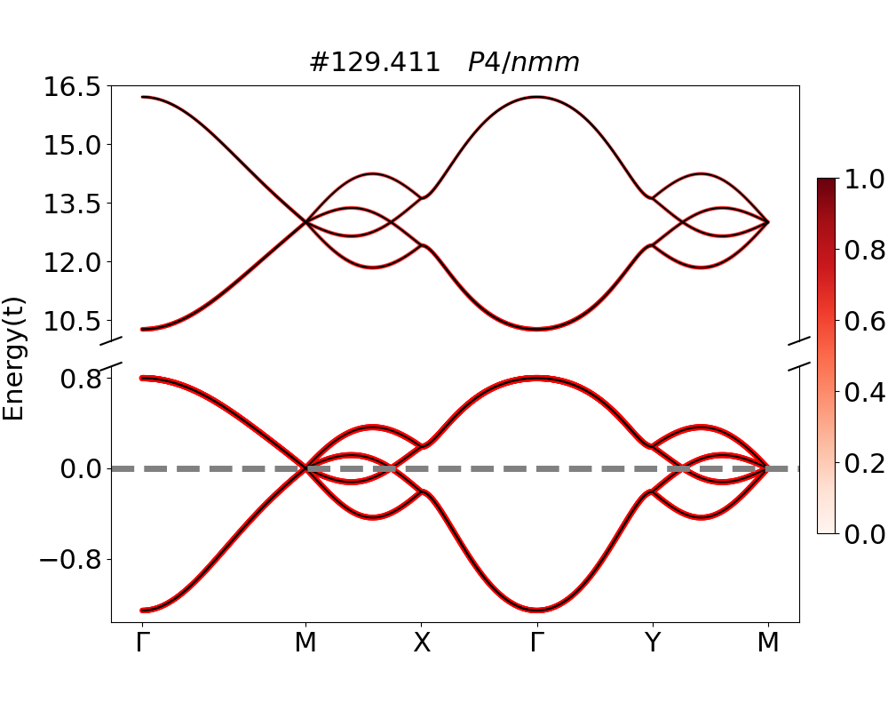
Figure 8: Band structure of the model Eq. (12) in MSG no. 129.411 ($P4/nmm$). Red color indicates the ratio of $f$ electrons in the states.

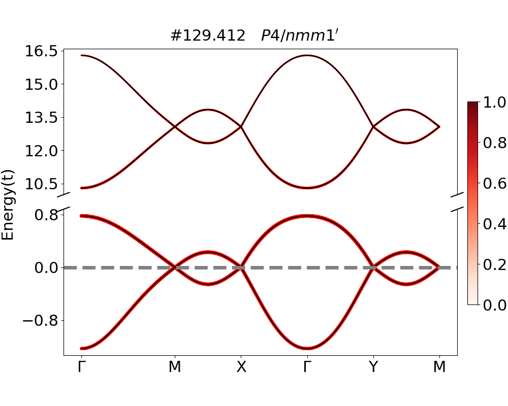
Figure 9: Band structure of the model Eq. (13) in MSG no. 129.412 ($P4/nmm1^{\prime}$).

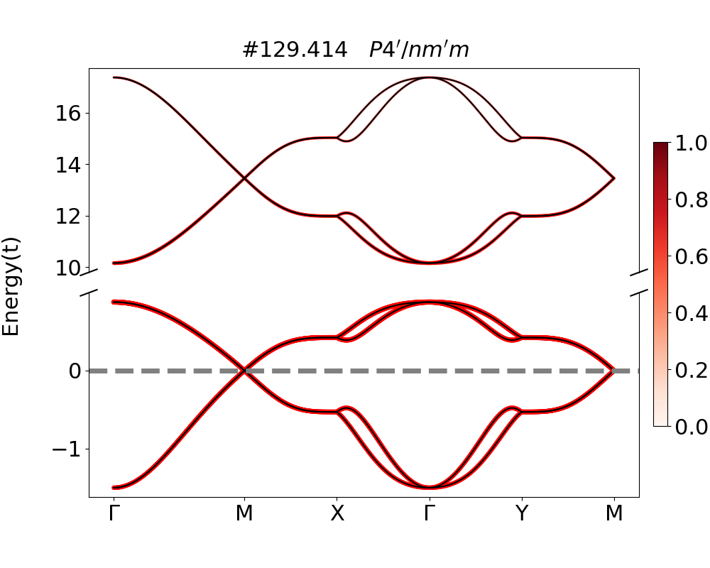
Figure 10: Band structure of the model Eq. (14) in MSG no. 129.411 ($P4^{\prime}/nm^{\prime}m$).

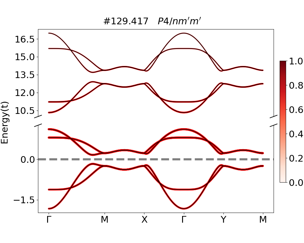
Figure 11: Band structure of the model Eq. (15) in MSG no. 129.417 ($P4/nm^{\prime}m^{\prime}$).

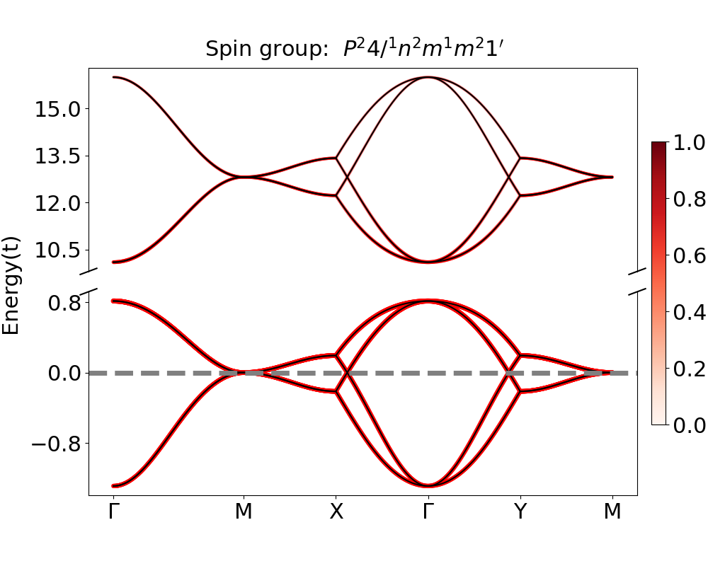
Figure 12: Band structure of the model Eq. (18) in spin group $P{}^{2}4/{}^{1}n{}^{1}m{}^{2}m{}^{2}1^{\prime}$.

MSG no. 129.415 ($P4^{\prime}/nmm^{\prime}$) and MSG no. 125.367 ($P4^{\prime}/nbm^{\prime}$) have many symmetries in common. They both have $C_{4}{\cal T}$ rotation about $(\frac{1}{4},\frac{1}{4},z)$ axis and inversion symmetry $\cal P$ centered at the origin. The difference is that $P4^{\prime}/nmm^{\prime}$ has screw symmetry $\{C_{2x}|\frac{1}{2}00\}$ while $P4^{\prime}/nbm^{\prime}$ has the glide symmetry $\{C_{2x}|0\frac{1}{2}0\}{\cal P}$. In the basis of $s$-orbitals in $2a$ Wyckoff position, the matrix representation is $\{C_{2x}|0\frac{1}{2}0\}=-i\sigma_{x}\tau_{0}$. The Hamiltonian of MSG no. 125.367 ($P4^{\prime}/nbm^{\prime}$) is

$$h^{(125.367)}({\mathbf{k}})= t\cos(\frac{k_{x}}{2})\cos(\frac{k_{y}}{2})\sigma_{0}\tau_{x}+t_{z}\sin(k_{z})\cos(\frac{k_{x}}{2})\cos(\frac{k_{y}}{2})\sigma_{0}\tau_{y}$$

$$+t_{SOC}\big{(}\sin(k_{x})\sigma_{x}-\sin(k_{y})\sigma_{y}\big{)}\tau_{z}$$

$$+t_{SOC}^{\prime}\sin(\frac{k_{x}}{2})\sin(\frac{k_{y}}{2})\sigma_{z}\tau_{x}$$

$$+t_{SOC}^{\prime\prime}\left(\cos(\frac{k_{x}}{2})\sin(\frac{k_{y}}{2})\sigma_{y}+\sin(\frac{k_{x}}{2})\cos(\frac{k_{y}}{2})\sigma_{x}\right)\tau_{y}$$ (16)

For comparison, we also list the Hamiltonian of MSG no. 129.415 ($P4^{\prime}/nmm^{\prime}$) here (Eq. (1) in the main text)

$$h^{(129.415)}({\mathbf{k}})= t\cos(\frac{k_{x}}{2})\cos(\frac{k_{y}}{2})\sigma_{0}\tau_{x}+t_{z}\sin(k_{z})\cos(\frac{k_{x}}{2})\cos(\frac{k_{y}}{2})\sigma_{0}\tau_{y}$$

$$+t_{SOC}\big{(}\sin(k_{x})\sigma_{y}+\sin(k_{y})\sigma_{x}\big{)}\tau_{z}$$

$$+t_{SOC}^{\prime}\sin(\frac{k_{x}}{2})\sin(\frac{k_{y}}{2})\sigma_{z}\tau_{x}$$

$$+t_{SOC}^{\prime\prime}\left(\cos(\frac{k_{x}}{2})\sin(\frac{k_{y}}{2})\sigma_{x}+\sin(\frac{k_{x}}{2})\cos(\frac{k_{y}}{2})\sigma_{y}\right)\tau_{y}$$ (17)

Therefore, when the parameters are chosen equally, the band structures (Fig. 2) and the Berry curvature distributions (Fig. 3) of the two models are identical.

We also present one example of the spin space group (for an introduction of spin space group, see Ref. [39]) $P{}^{2}4/{}^{1}n{}^{1}m{}^{2}m{}^{2}1^{\prime}$ in Fig. 12. It is generated by spin group symmetries $[C_{2}||C_{4}]$, $[E||{\cal P}]$, $[C_{2}||\{C_{2x}|\frac{1}{2}00\}]$, and $[C_{2}||E]{\cal T}$, where $[A||B]$ indicates the symmetry is composed of a symmetry $A$ acting in the spin space and a symmetry $B$ acting in the real space. The Hamiltonian of this group is

$$h^{\text{spin group}}({\mathbf{k}})= t\cos(\frac{k_{x}}{2})\cos(\frac{k_{y}}{2})\sigma_{0}\tau_{x}+t_{z}\sin(k_{z})\cos(\frac{k_{x}}{2})\cos(\frac{k_{y}}{2})\sigma_{0}\tau_{y}$$

$$+\big{(}\cos(k_{x})-\cos(k_{y})\big{)}\sigma_{y}\big{(}t_{SOC1}\tau_{z}+t_{SOC2}\tau_{x}\big{)}$$ (18)

The band structure of this model is shown in Fig. 12, where the symmetry enforced Dirac point and hourglass Weyl nodal lines coexist.

Appendix D MSGs in SG no. 125 and SG no. 31 families

MSG #	BNS	FM	AFM	Hall response	Crossing type
125.363	$P4/nbm$		✓	3rd- order	Dirac
125.364	$P4/nbm1^{\prime}$				Dirac
125.365	$P4/n^{\prime}bm$		✓
125.366	$P4^{\prime}/nb^{\prime}m$		✓	3rd- order	Dirac
125.367	$P4^{\prime}/nbm^{\prime}$		✓	3rd- order	hourglass Weyl nodal line
125.368	$P4^{\prime}/n^{\prime}b^{\prime}m$		✓		Dirac
125.369	$P4/nb^{\prime}m^{\prime}$	✓	✓	1st-order
125.370	$P4^{\prime}/n^{\prime}bm^{\prime}$		✓		hourglass Weyl nodal line
125.371	$P4/n^{\prime}b^{\prime}m^{\prime}$		✓		hourglass Weyl nodal line
125.372	$P_{c}4/nbm$		✓		Dirac
125.373	$P_{C}4/nbm$		✓		Dirac
125.374	$P_{I}4/nbm$		✓		double Dirac

Table 3: MSGs of space group no. 125 family. We use BNS setting to denote the MSGs . The magnetic orderings compatible with each MSG are marked with $\checkmark$. Blank means the magnetic ordering is not compatible with the group. The leading order Hall response of each group is listed. Blank means no Hall response of any order is permitted. The crossing types for bands from $s$-orbitals at $2a$ Wyckoff positions are listed. Blank means no symmetry-enforced Dirac point, hourglass Weyl nodal line, or double Dirac point exists in the group.

MSG #	BNS	FM	AFM	Hall response	Crossing type
31.123	$Pmn2_{1}$		✓	2nd-order
31.124	$Pmn2_{1}1^{\prime}$			2nd-order	Dirac
31.125	$Pm^{\prime}n2_{1}^{\prime}$	✓	✓	1st-order
31.126	$Pmn^{\prime}2_{1}^{\prime}$	✓	✓	1st-order
31.127	$Pm^{\prime}n^{\prime}2_{1}$	✓	✓	1st-order
31.128	$P_{a}mn2_{1}$		✓	2nd-order	Dirac
31.129	$P_{b}mn2_{1}$		✓	2nd-order	Dirac
31.130	$P_{c}mn2_{1}$		✓	2nd-order	hourglass Weyl nodal line
31.131	$P_{A}mn2_{1}$		✓	2nd-order	hourglass Weyl nodal line
31.132	$P_{B}mn2_{1}$		✓	2nd-order
31.133	$P_{C}mn2_{1}$		✓	2nd-order	Dirac
31.134	$P_{I}mn2_{1}$		✓	2nd-order

Table 4: MSGs of space group no. 31 family. The interpretation of this table is the same as Table 1.

SG 125 family is very similar to SG 129 family. As we have discussed in the previous section, they differ by the two-fold rotation symmetry about $x$ and $y$-axis. Therefor, the compatible magnetic ordering and the corresponding Hall responses are identical in Table 1 and Table 3. However, the symmetry enforced crossings can be different as we listed in Table 3. In particular, in MSG no. 125.374 ($P_{I}4/nbm$) there is a double Dirac point at $(\pi,\pi,\pi)$ due to the interplay between anti-unitary symmetries and nonsymmorphic groups.

For the 31 family, MSGs no. 31.125-31.127 are compatible with FM ordering while all MSGs in this family except no. 31.124 are compatible with certain AFM ordering. MSGs no. 31.123, no. 31.124 and no.31.128-31.134 have 2nd-order responses as the leading order.

For MSG no. 31.130 and no. 31.131, the compatibility conditions require the following irreps connectivity: $\overline{R}_{2}\overline{R}_{4}(2)\rightarrow\overline{N}_{3}(1)\oplus\overline{N}_{4}(1)$, $\overline{R}_{3}\overline{R}_{5}(2)\rightarrow\overline{N}_{3}(1)\oplus\overline{N}_{4}(1)$, and $\overline{S}_{2}\overline{S}_{5}(2)\rightarrow\overline{N}_{4}(1)\oplus\overline{N}_{4}(1)$, $\overline{S}_{3}\overline{S}_{4}(2)\rightarrow\overline{N}_{3}(1)\oplus\overline{N}_{3}(1)$, where $N=(u,\pi,w)$, $R=(\pi,\pi,\pi)$, $S=(\pi,\pi,0)$. Therefore, there are symmetry enforced hourglass Weyl nodal lines in the $k_{y}=\pi$ plane.

Appendix E Physical properties of materials candidates

Materials	MSG #	BNS	MPG	Hall response	$T_{curie}$	$T_{N}$	$T_{K}$	$\rho\rm(\mu\Omega/cm)$	$\gamma\rm(mJ/K^{2}mol)$
$\rm CeMn_{2}Ge_{4}O_{12}$ [40, 30]	125.367	$P4^{\prime}/nbm^{\prime}$	$4^{\prime}/mmm^{\prime}$	3rd- order		7.6K
$\rm Ce_{4}Ge_{3}$ [31]	122.333	$I\bar{4}2d$	$\bar{4}2m$	2nd-order		6K,12K
$\rm Ce_{4}Sb_{3}$ [32]	122.336	$I\bar{4}^{\prime}2d^{\prime}$	$\bar{4}^{\prime}2m^{\prime}$	2nd-order	5K	$<$ 14K
$\rm Ce_{3}NIn$ [33]	117.305	$P_{C}\bar{4}b2$	$\bar{4}2m1^{\prime}$	2nd-order		9K
$\rm CeNiAsO$ [34]	4.10	$P_{a}2_{1}$	$21^{\prime}$	2nd-order		8.7K	15K	$<10$  [41]	$203$
$\rm CeSbTe$ [42]	4.10	$P_{a}2_{1}$	$21^{\prime}$	2nd-order		2.7K			$10$
$\rm CeAuSb_{2}$ [35, 36]	39.201	$A_{b}Bm2$	$mm21^{\prime}$	2nd-order		6.5K	10K	$20\sim 60$	$>50$
$\rm CeCuGa_{3}$ [37]	44.230	$Imm21^{\prime}$	$mm21^{\prime}$	2nd-order	0.4K	1.9K	4-6K		$>99$
$\rm CeCu_{2}Ge_{2}$ [38]	44.230	$Imm21^{\prime}$	$mm21^{\prime}$	2nd-order		4.1K	10K	$<120$ [43]	$1400$
$\rm CeFeAsO$ [44, 45]	21.41	$C22^{\prime}2^{\prime}$	$22^{\prime}2^{\prime}$	1st-order		4K	10K	$2.8\times 10^{3}$ [46]	$800$ [47]
$\rm CeMn_{2}Ge_{2}$ [48]	97.154	$I42^{\prime}2^{\prime}$	$42^{\prime}2^{\prime}$	1st-order
$\rm Ce_{2}PdGe_{3}$ [49]	6.20	$Pm^{\prime}$	$m^{\prime}$	1st-order		30K		$200$	$50$ [50]
$\rm CeCoGe_{3}$ [40]	107.231	$I4m^{\prime}m^{\prime}$	$4m^{\prime}m^{\prime}$	1st-order					$111$ [51]

Table 5: Material Candidates of $\rm Ce$ based materials with non-vanishing (nonlinear) Hall responses. The transition temperatures of magnetic ordering due to $f$ electrons in $\rm Ce$ are listed. The resistivity and Sommerfeld constant in heat capacity are also listed. $\rm CeNiAsO$ and $\rm CeFeAsO$ are reported to have the AFM orders from $d$ electrons. The Néel temperature of this order for $\rm CeFeAsO$ is $T_{N}=130$K. $\rm CeMn_{2}Ge_{2}$ is reported to have FM order from $d$ electrons, with Curie temperature $T_{curie}>300$K.

As explained in the main text, we have summarized the materials candidate with nonvanishing anomalous Hall effect but could not identify any convincing material candidate for MWKSM from the established databases. In particular, we have searched MAGNDATA [52, 53]. $\rm CeNiAsO$ potentially has a 2nd-order response, hourglass Weyl nodal lines and large Sommerfeld coefficient showing the existence of strong interactions. However, for the other materials, future experimentas are needed to establish that they feature both $d$ electron AFM order and topological semimetallic phases. We list the information about physical properties collected from literature in Table 5.

References

- Keimer and Moore [2017] B. Keimer and J. E. Moore, Nat. Phys. 13, 1045 (2017).
- Paschen and Si [2021] S. Paschen and Q. Si, Nat. Rev. Phys. 3, 9 (2021).
- Lai et al. [2018] H.-H. Lai, S. E. Grefe, S. Paschen, and Q. Si, Proceedings of the National Academy of Sciences 115, 93 (2018), https://www.pnas.org/doi/pdf/10.1073/pnas.1715851115 .
- Dzsaber et al. [2017] S. Dzsaber, L. Prochaska, A. Sidorenko, G. Eguchi, R. Svagera, M. Waas, A. Prokofiev, Q. Si, and S. Paschen, Phys. Rev. Lett. 118, 246601 (2017).
- Armitage et al. [2018] N. P. Armitage, E. J. Mele, and A. Vishwanath, Rev. Mod. Phys. 90, 015001 (2018).
- Son and Spivak [2013] D. T. Son and B. Z. Spivak, Phys. Rev. B 88, 104412 (2013).
- Hosur and Qi [2013] P. Hosur and X. Qi, Comptes Rendus Physique 14, 857 (2013), topological insulators / Isolants topologiques.
- Zyuzin and Burkov [2012] A. A. Zyuzin and A. A. Burkov, Phys. Rev. B 86, 115133 (2012).
- Yan and Felser [2017] B. Yan and C. Felser, Annual Review of Condensed Matter Physics 8, 337 (2017), https://doi.org/10.1146/annurev-conmatphys-031016-025458 .
- Elcoro et al. [2021] L. Elcoro, B. J. Wieder, Z. Song, Y. Xu, B. Bradlyn, and B. A. Bernevig, Nature Communications 12, 5965 (2021).
- Cano and Bradlyn [2021] J. Cano and B. Bradlyn, Annual Review of Condensed Matter Physics 12, 225 (2021), https://doi.org/10.1146/annurev-conmatphys-041720-124134 .
- Kirchner et al. [2020] S. Kirchner, S. Paschen, Q. Chen, S. Wirth, D. Feng, J. D. Thompson, and Q. Si, Rev. Mod. Phys. 92, 011002 (2020).
- Hewson [1997] A. C. Hewson, The Kondo problem to heavy fermions (Cambridge university press, 1997).
- Chen et al. [2022] L. Chen, C. Setty, H. Hu, M. G. Vergniory, S. E. Grefe, L. Fischer, X. Yan, G. Eguchi, A. Prokofiev, S. Paschen, J. Cano, and Q. Si, Nature Physics 18, 1341 (2022).
- Grefe et al. [2020] S. E. Grefe, H.-H. Lai, S. Paschen, and Q. Si, Phys. Rev. B 101, 075138 (2020).
- Grefe et al. [2020] S. E. Grefe, H.-H. Lai, S. Paschen, and Q. Si, arXiv e-prints , arXiv:2012.15841 (2020), arXiv:2012.15841 [cond-mat.str-el] .
- Hu et al. [2021] H. Hu, L. Chen, C. Setty, M. Garcia-Diez, S. E. Grefe, A. Prokofiev, S. Kirchner, M. G. Vergniory, S. Paschen, J. Cano, and Q. Si, arXiv e-prints , arXiv:2110.06182 (2021), arXiv:2110.06182 [cond-mat.str-el] .
- Dzsaber et al. [2021] S. Dzsaber, X. Yan, M. Taupin, G. Eguchi, A. Prokofiev, T. Shiroka, P. Blaha, O. Rubel, S. E. Grefe, H.-H. Lai, Q. Si, and S. Paschen, Proceedings of the National Academy of Sciences 118, e2013386118 (2021), https://www.pnas.org/doi/pdf/10.1073/pnas.2013386118 .
- Dzsaber et al. [2022] S. Dzsaber, D. A. Zocco, A. McCollam, F. Weickert, R. McDonald, M. Taupin, G. Eguchi, X. Yan, A. Prokofiev, L. M. K. Tang, B. Vlaar, L. E. Winter, M. Jaime, Q. Si, and S. Paschen, Nature Communications 13, 5729 (2022).
- Bradley and Cracknell [2009] C. J. Bradley and A. P. Cracknell, The Mathematical Theory Of Symmetry In Solids: Representation theory for point groups and space groups (Oxford University Press, 2009).
- Klemenz et al. [2020a] S. Klemenz, L. Schoop, and J. Cano, Phys. Rev. B 101, 165121 (2020a).
- Klemenz et al. [2019] S. Klemenz, S. Lei, and L. M. Schoop, Annual Review of Materials Research 49, 185 (2019), https://doi.org/10.1146/annurev-matsci-070218-010114 .
- Klemenz et al. [2020b] S. Klemenz, A. K. Hay, S. M. L. Teicher, A. Topp, J. Cano, and L. M. Schoop, Journal of the American Chemical Society, Journal of the American Chemical Society 142, 6350 (2020b).
- Lei et al. [2023] S. Lei, K. Allen, J. Huang, J. M. Moya, T. C. Wu, B. Casas, Y. Zhang, J. S. Oh, M. Hashimoto, D. Lu, J. Denlinger, C. Jozwiak, A. Bostwick, E. Rotenberg, L. Balicas, R. Birgeneau, M. S. Foster, M. Yi, Y. Sun, and E. Morosan, Nature Communications 14, 5812 (2023).
- Zhang et al. [2023] C.-P. Zhang, X.-J. Gao, Y.-M. Xie, H. C. Po, and K. T. Law, Phys. Rev. B 107, 115142 (2023).
- Fang et al. [2023] Y. Fang, J. Cano, and S. A. A. Ghorashi, arXiv e-prints , arXiv:2310.11489 (2023), arXiv:2310.11489 [cond-mat.mes-hall] .
- Sodemann and Fu [2015] I. Sodemann and L. Fu, Phys. Rev. Lett. 115, 216806 (2015).
- Wu et al. [2019a] W. Wu, Y. Jiao, S. Li, X.-L. Sheng, Z.-M. Yu, and S. A. Yang, Phys. Rev. Mater. 3, 054203 (2019a).
- [29] Supplementary material .
- Xu et al. [2017] D. Xu, M. Avdeev, P. D. Battle, and X.-Q. Liu, Inorganic Chemistry, Inorganic Chemistry 56, 2750 (2017).
- Morozkin et al. [2009] A. Morozkin, O. Isnard, R. Nirmala, and S. Malik, Journal of Alloys and Compounds 486, 497 (2009).
- Nirmala et al. [2009] R. Nirmala, A. Morozkin, O. Isnard, and A. Nigam, Journal of Magnetism and Magnetic Materials 321, 188 (2009).
- Gäbler et al. [2008] F. Gäbler, W. Schnelle, A. Senyshyn, and R. Niewa, Solid State Sciences 10, 1910 (2008), molecular Metals, Superconductors and Magnets.
- Wu et al. [2019b] S. Wu, W. A. Phelan, L. Liu, J. R. Morey, J. A. Tutmaher, J. C. Neuefeind, A. Huq, M. B. Stone, M. Feygenson, D. W. Tam, B. A. Frandsen, B. Trump, C. Wan, S. R. Dunsiger, T. M. McQueen, Y. J. Uemura, and C. L. Broholm, Phys. Rev. Lett. 122, 197203 (2019b).
- Waite et al. [2022] R. Waite, F. Orlandi, D. A. Sokolov, R. A. Ribeiro, P. C. Canfield, P. Manuel, D. D. Khalyavin, C. W. Hicks, and S. M. Hayden, Phys. Rev. B 106, 224415 (2022).
- Zhao et al. [2016] L. Zhao, E. A. Yelland, J. A. N. Bruin, I. Sheikin, P. C. Canfield, V. Fritsch, H. Sakai, A. P. Mackenzie, and C. W. Hicks, Phys. Rev. B 93, 195124 (2016).
- Anand et al. [2021] V. K. Anand, A. Fraile, D. T. Adroja, S. Sharma, R. Tripathi, C. Ritter, C. de la Fuente, P. K. Biswas, V. G. Sakai, A. del Moral, and A. M. Strydom, Phys. Rev. B 104, 174438 (2021).
- Knopp et al. [1989] G. Knopp, A. Loidl, K. Knorr, L. Pawlak, M. Duczmal, R. Caspary, U. Gottwick, H. Spille, F. Steglich, and A. P. Murani, Zeitschrift für Physik B Condensed Matter 77, 95 (1989).
- Litvin and Opechowski [1974] D. Litvin and W. Opechowski, Physica 76, 538 (1974).
- Xu et al. [2020] Y. Xu, L. Elcoro, Z.-D. Song, B. J. Wieder, M. G. Vergniory, N. Regnault, Y. Chen, C. Felser, and B. A. Bernevig, Nature 586, 702 (2020).
- Luo et al. [2014] Y. Luo, L. Pourovskii, S. E. Rowley, Y. Li, C. Feng, A. Georges, J. Dai, G. Cao, Z. Xu, Q. Si, and N. P. Ong, Nature Materials 13, 777 (2014).
- Schoop et al. [2018] L. M. Schoop, A. Topp, J. Lippmann, F. Orlandi, L. Müchler, M. G. Vergniory, Y. Sun, A. W. Rost, V. Duppel, M. Krivenkov, S. Sheoran, P. Manuel, A. Varykhalov, B. Yan, R. K. Kremer, C. R. Ast, and B. V. Lotsch, Science Advances 4, eaar2317 (2018), https://www.science.org/doi/pdf/10.1126/sciadv.aar2317 .
- Rauchschwalbe et al. [1985] U. Rauchschwalbe, U. Gottwick, U. Ahlheim, H. Mayer, and F. Steglich, Journal of the Less Common Metals 111, 265 (1985).
- Zhao et al. [2008] J. Zhao, Q. Huang, C. de la Cruz, S. Li, J. W. Lynn, Y. Chen, M. A. Green, G. F. Chen, G. Li, Z. Li, J. L. Luo, N. L. Wang, and P. Dai, Nature Materials 7, 953 (2008).
- Dai et al. [2009] J. Dai, J.-X. Zhu, and Q. Si, Phys. Rev. B 80, 020505 (2009).
- Chen et al. [2008] G. F. Chen, Z. Li, D. Wu, G. Li, W. Z. Hu, J. Dong, P. Zheng, J. L. Luo, and N. L. Wang, Phys. Rev. Lett. 100, 247002 (2008).
- Luo et al. [2010] Y. Luo, Y. Li, S. Jiang, J. Dai, G. Cao, and Z.-a. Xu, Phys. Rev. B 81, 134422 (2010).
- Welter et al. [1995] R. Welter, G. Venturini, E. Ressouche, and B. Malaman, Journal of Alloys and Compounds 218, 204 (1995).
- Cedervall et al. [2016] J. Cedervall, P. Beran, M. Vennström, T. Danielsson, S. Ronneteg, V. Höglin, D. Lindell, O. Eriksson, G. André, Y. Andersson, P. Nordblad, and M. Sahlberg, Journal of Solid State Chemistry 237, 343 (2016).
- Baumbach et al. [2015] R. E. Baumbach, A. Gallagher, T. Besara, J. Sun, T. Siegrist, D. J. Singh, J. D. Thompson, F. Ronning, and E. D. Bauer, Phys. Rev. B 91, 035102 (2015).
- Pecharsky et al. [1993] V. K. Pecharsky, O.-B. Hyun, and K. A. Gschneidner, Phys. Rev. B 47, 11839 (1993).
- Gallego et al. [2016a] S. V. Gallego, J. M. Perez-Mato, L. Elcoro, E. S. Tasci, R. M. Hanson, K. Momma, M. I. Aroyo, and G. Madariaga, Journal of Applied Crystallography 49, 1750 (2016a).
- Gallego et al. [2016b] S. V. Gallego, J. M. Perez-Mato, L. Elcoro, E. S. Tasci, R. M. Hanson, M. I. Aroyo, and G. Madariaga, Journal of Applied Crystallography 49, 1941 (2016b).