A new HOC scheme for computation of flow and heat transfer in nonuniform polar grids

Abstract

In this work, a higher order compact (HOC) discretization is developed on the nonuniform polar grid. The discretization conceptualized using the unsteady convection-diffusion equation (CDE) is further extended to flow problems governed by the Navies-Stokes (N-S) equations as well as the Boussinesq equations. The scheme developed here combines the advantages of body-fitted mesh with grid clustering, thereby making it efficient to capture flow gradients on polar grids. The scheme carries a spatial convergence of order three with temporal order of convergence being almost two. Diverse flow problems are being investigated using the scheme. Apart from two verification studies we validate the scheme by time marching simulation for the benchmark problem of driven polar cavity and the problem of natural convection in the horizontal concentric annulus. In the process, a one-sided approximation for the Neumann boundary condition for vorticity is also presented. Finally, the benchmark problem of forced convection around a circular cylinder is tackled. The results obtained in this study are analyzed and compared with the well-established numerical and experimental data wherever available in the literature. The newly developed scheme is found to generate accurate solutions in each case.

1 Introduction

Fluid flow problems involving circular geometries have attracted a great deal of attention over the years owing to their theoretical significance and physical relevance. For such importance, higher order compact (HOC) schemes have been developed on the cylindrical polar coordinates. Preliminary works to develop HOC schemes on cylindrical polar coordinate systems mostly focused on the Poisson equation and uniform grids [1, 2, 3, 4, 5, 6]. Here it is important to note that in polar coordinates Poisson equation involves variable coefficients and thus the above-mentioned works involved significant endeavors and were not mere extension of the works done in Cartesian coordinates. Additionally, a valid discretization at singularity $r=0$ is necessary. Subsequently, considerable efforts could be found in the literature on HOC discretization of N-S equations in the body-fitted polar coordinate system [7, 8, 9, 10, 11]. In the year 2005 Sanyasiraju and Manjula [7] proposed a higher order semicompact scheme to solve the flow past an impulsively started circular cylinder. The authors used a wider stencil to discretize a few terms of the governing equation rendering semicompactness to the scheme. This strategy also helped alleviate challenges associated with the variable coefficients of the second order derivative. Subsequently, Kalita and Ray [8] developed a temporally second order and spatially third order accurate HOC scheme for streamfunction-vorticity $(\psi-\omega)$ formulation of unsteady N-S equation. As the authors worked with a modified differential equation the resulting difference equation carried a higher order of singularity. The scheme was specially adapted to simulate incompressible flow past a circular cylinder directly on nonuniform polar grids. A rather straightforward adaptation of this scheme for steady convection-diffusion equation (CDE) can be found in [9]. In the year 2013, the pioneering work on compact difference schemes for the pure streamfunction formulation of N-S equations in polar coordinates was reported by Yu and Tian [10]. The authors here worked with the steady biharmonic equation in polar coordinates. The scheme developed therein is of second order accuracy and carries streamfunction and its first derivatives as the unknown variables. Of late Das et al. [11] also worked with steady second order equation with variable coefficients in polar coordinates and introduced a third order accurate HOC scheme. The scheme claimed to be implemented on a nonuniform grid used an implicit form of first order derivatives and was successful in simulating steady incompressible flows. It is clear from the above discussion that classical HOC discretization of transient generalized second order PDE with variable coefficients in polar coordinates has not been attempted apart from the work of Kalita and Ray [8] on $\psi-\omega$ form of the N-S equations, whose extension to other governing equations such as the Boussinesq equation is not immediate. Additionally, it is intriguing to notice that developed HOC schemes in polar coordinates have been traditionally used to handle the nonuniformity of grids in radial direction only. However, heat and fluid flow problems are often associated with generation of steep gradients of streamfunction and vorticity near the bluff body or domain boundary walls, and as such grid clustering in all directions should be economical.

In this work, we intend to develop a new transient HOC formulation that can simulate fluid as well as heat transfer problems directly in polar coordinates. The scheme conceived in the process must be generalizable to approximate second order equations with variable coefficients in polar coordinates and should be efficient for circular geometries. Starting with a second order PDE with variable coefficients, we advocate a discretization strategy amenable for extension to a nonlinear system of N-S equations and beyond. Additionally, we adopt the philosophy of nonuniform grids for accurate resolution of complex flow problems. We look forward to combining the virtues of Padé approximation of first order derivatives on nonuniform grids with variable coefficients and compact discretization of higher order derivatives in terms of flow variables and their first order gradients. Theoretically, the scheme has a temporal convergence of second order and a spatial convergence of order three. The scheme developed here leads to stable higher order discretization in conjunction with both Dirichlet and convective boundary conditions. The formulation is validated by applying it to the problem of an unsteady Gaussian pulse governed by the linear CDE. This problem is equipped with known analytical solution, which helps in error analysis. The spatial and temporal order of convergence are also established during this process. However, to comprehend the robustness and adaptability of this new scheme, we carry out the simulations for benchmark problems of both flow and heat transfer, namely the flow inside a driven polar cavity, natural convection inside a circular annulus, and forced convection around a stationary circular cylinder. These flows are governed by N-S equations and Boussinesq equations, both the equation being cast in transient incompressible form. The $(\psi-\omega)$ formulation of these coupled nonlinear PDE’s are conformed for the present computation.

The rest of this manuscript is organised in four sections. In section 2 compact discretization of transient CDE on cylindrical polar coordinate grids. Section 3 deals with solution of algebraic system of equations. The four test cases are described in the section 4 and finally, section 5 gives a gist of the whole work.

2 Mathematical formulation and discretization procedure

In the nonrectangular domain $\Omega=[a_{r},b_{r}]\times[a_{\theta},b_{\theta}]$, the polar $(r,\theta)$ form of the CDE is

$$a\phi_{t}-\phi_{rr}-\frac{1}{r^{2}}\phi_{\theta\theta}+c_{1}(r,\theta,t)\phi_{r}+c_{2}(r,\theta,t)\phi_{\theta}=f(r,\theta,t),$$ (1)

where $a>0$ is a constant; $c_{1}$ and $c_{2}$ are convection coefficients.

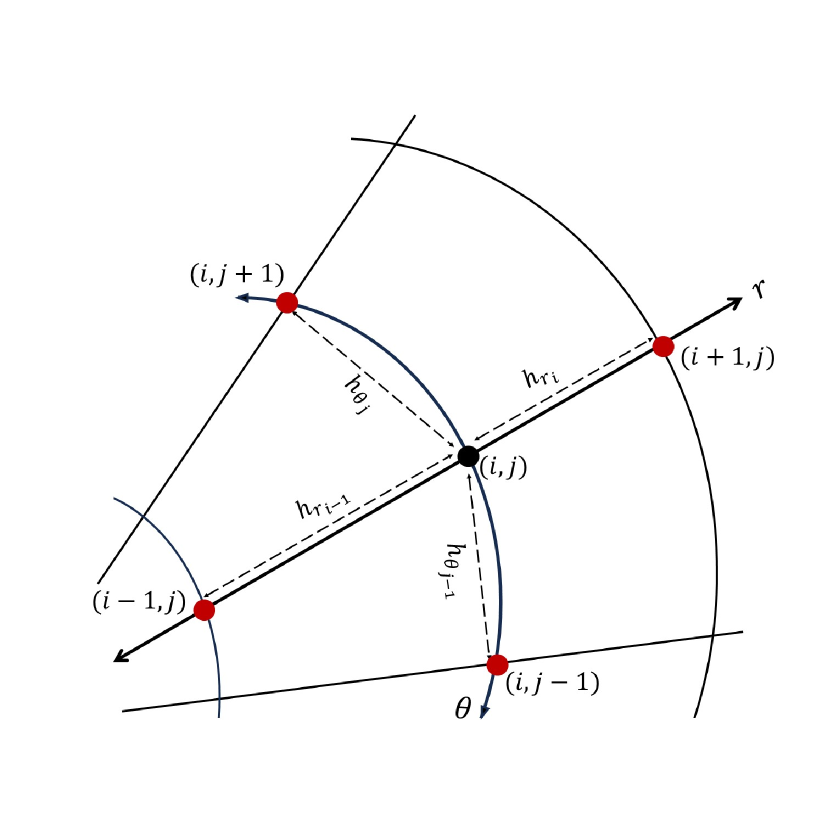
a

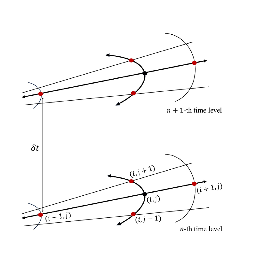
b

Figure 1: (a) Projection of nonuniform computational stencil in $(r,\theta)$ plane and (b) Nonuniform computational stencil in $(r,\theta,t)$ hyper-plane.

We discretize the domain by considering $a_{r}=r_{1}<r_{2}<r_{3}<\cdots<r_{n_{r}}=b_{r}$ and $a_{\theta}=\theta_{1}<\theta_{2}<\theta_{3}<\cdots<\theta_{n_{\theta}}=b_{\theta}$ where lengths between two consecutive $r_{i}$’s, $i=1,2,3,\dots,n_{r}$ and $\theta_{j}$’s, $j=1,2,3,\dots,n_{\theta}$ may be unequal. A typical stencil can be seen in fig. 1. The figure depicts the grid points at the $n$-th and $(n+1)$-th time level as well. We define the mesh sizes along radial and tangential directions to be

$$h_{r_{i}} =r_{i+1}-r_{i},\quad i\in{1,2,3,\dots,n_{r}-1},$$

$$h_{\theta_{j}} =\theta_{j+1}-\theta_{j},\quad j\in{1,2,3,\dots,n_{\theta}-1}.$$

For the sufficiently smooth transport variable $\phi(r,\theta)$, the first and second order finite difference operator $\delta_{r}$ and $\delta_{rr}$ in the radial direction are defined as,

$$\delta_{r}\phi_{i,j}=\frac{1}{h_{i}+h_{i-1}}\left(\phi_{i+1,j}-\phi_{i-1,j}\right)$$ (2)

and

$$\delta_{rr}\phi_{i,j}=\frac{2}{h_{r_{i}}+h_{r_{i-1}}}\left[\frac{\phi_{i+1,j}}{h_{r_{i}}}+\frac{\phi_{i-1,j}}{h_{r_{i-1}}}-\left(\frac{1}{h_{r_{i}}}+\frac{1}{h_{r_{i-1}}}\right)\phi_{i,j}\right]$$ (3)

respectively, where $\phi_{i,j}$ denotes $\phi(r_{i},\theta_{j})$. The first and second order partial derivatives of $\phi$ along $r$-direction at a point $(r_{i},\theta_{j})$ lying inside the reference domain can be approximated using Taylor series expansion as

$$\partial_{r}\phi_{i,j}=\delta_{r}\phi_{i,j}-\frac{1}{2}\left(h_{r_{i}}-h_{r_{i-1}}\right)\partial_{rr}\phi_{i,j}-\frac{1}{6}\left(\frac{h_{r_{i}}^{3}+h_{r_{i-1}}^{3}}{h_{r_{i}}+h_{r_{i-1}}}\right)\partial_{rrr}\phi_{i,j}+\mathcal{O}\left(\frac{h_{r_{i}}^{4}-h_{r_{i-1}}^{4}}{h_{r_{i}}+h_{r_{i+1}}}\right),$$ (4)

and

$$\partial_{rr}\phi_{i,j}=\delta_{rr}\phi_{i,j}-\frac{1}{3}\left(h_{r_{i}}-h_{r_{i-1}}\right)\partial_{rrr}\phi_{i,j}-\frac{1}{12}\left(\frac{h_{r_{i}}^{3}+h_{r_{i-1}}^{3}}{h_{r_{i}}+h_{r_{i-1}}}\right)\partial_{rrrr}\phi_{i,j}+\mathcal{O}\left(\frac{h_{r_{i}}^{4}-h_{r_{i-1}}^{4}}{h_{r_{i}}+h_{r_{i+1}}}\right).$$ (5)

Combining equations 4 and 5, we arrive at the third order accurate approximation of second order derivative which is given as

$$\partial_{rr}\phi_{i,j}= 2\left(\frac{2(h_{r_{i}}^{2}-h_{r_{i}}h_{r_{i-1}}+h_{r_{i-1}}^{2})}{h_{r_{i}}^{2}+h_{r_{i-1}}^{2}}\delta_{rr}\phi_{i,j}-\frac{h_{r_{i}}^{2}-h_{r_{i}}h_{r_{i-1}}+h_{r_{i-1}}^{2}}{h_{r_{i}}^{2}+h_{r_{i-1}}^{2}}\delta_{r}\phi_{r_{i,j}}\right.$$ (6)

$$\left.-\frac{h_{r_{i}}-h_{r_{i-1}}}{h_{r_{i}}^{2}+h_{r_{i-1}}^{2}}\delta_{r}\phi_{i,j}+\frac{h_{r_{i}}-h_{r_{i-1}}}{h_{r_{i}}^{2}+h_{r_{i-1}}^{2}}\phi_{r_{i,j}}\right)+\mathcal{O}\left(\frac{h_{r_{i}}^{4}-h_{r_{i-1}}^{4}}{h_{r_{i}}+h_{r_{i-1}}}\right).$$

The analogous approximation along the tangential direction can be obtained as

$$\partial_{\theta\theta}\phi_{i,j}= 2\left(\frac{2(h_{\theta_{j}}^{2}-h_{\theta_{j}}h_{\theta_{j-1}}+h_{\theta_{j-1}}^{2})}{h_{\theta_{j}}^{2}+h_{\theta_{j-1}}^{2}}\delta_{\theta\theta}\phi_{i,j}-\frac{h_{\theta_{j}}^{2}-h_{\theta_{j}}h_{\theta_{j-1}}+h_{\theta_{j-1}}^{2}}{h_{\theta_{j}}^{2}+h_{\theta_{j-1}}^{2}}\delta_{\theta}\phi_{\theta_{i,j}}\right.$$ (7)

$$\left.-\frac{h_{\theta_{j}}-h_{\theta_{j-1}}}{h_{\theta_{j}}^{2}+h_{\theta_{j-1}}^{2}}\delta_{\theta}\phi_{i,j}+\frac{h_{\theta_{j}}-h_{\theta_{j-1}}}{h_{\theta_{j}}^{2}+h_{\theta_{j-1}}^{2}}\phi_{\theta_{i,j}}\right)+\mathcal{O}\left(\frac{h_{\theta_{j}}^{4}-h_{\theta_{j-1}}^{4}}{h_{\theta_{j}}+h_{\theta_{j-1}}}\right).$$

Once these approximations are achieved they are used in the CDE (1) to obtain its semi discrete form around the node $(i,j)$, which may be written as,

$$a\left.\phi_{t}\right|_{i,j}+[\mathcal{A}\phi]_{i,j}=f_{i,j}.$$ (8)

The operator $\mathcal{A}$ is defined as,

$$\mathcal{A}\phi_{i,j}= -\left(2A_{1}\delta_{r}^{2}+\frac{2A_{2}}{r_{i}^{2}}\delta_{\theta}^{2}+\frac{A_{3}}{h_{r_{i-1}}}\delta_{r}+\frac{A_{4}}{r_{i}^{2}h_{\theta_{j-1}}}\delta_{\theta}\right)\phi_{i,j}$$ (9)

$$+\left(A_{1}\delta_{r}+\frac{A_{3}}{h_{r_{i-1}}}+c_{1}\right)\phi_{r_{i,j}}+\left(A_{2}\delta_{\theta}+\frac{A_{4}}{r_{i}^{2}h_{\theta_{j-1}}}+\frac{c_{2}}{r_{i}^{2}}\right)\phi_{\theta_{i,j}}$$

which is accompanied by the coefficients,

$$A_{1}=\frac{2(1-\alpha_{r}+\alpha_{r}^{2})}{(1+\alpha_{r}^{2})},\quad A_{2}=\frac{2(1-\alpha_{\theta}+\alpha_{\theta}^{2})}{(1+\alpha_{\theta}^{2})},\quad A_{3}=\frac{2(1-\alpha_{r})}{(1+\alpha_{r}^{2})},\quad A_{4}=\frac{2(1-\alpha_{\theta})}{(1+\alpha_{\theta}^{2})}.$$

In the coefficients $A_{1}$, $A_{2}$, $A_{3}$ and $A_{4}$ the terms $\alpha_{r}$ and $\alpha_{\theta}$ are used to replace the arrays $\alpha_{r_{i}}$, $i\in{1,2,3,\dots,n_{r}-2}$ and $\alpha_{\theta_{j}}$, $j\in{1,2,3,\dots,n_{\theta}-2}$ respectively, which are characterized as follows,

$$\alpha_{r_{i-1}} =h_{r_{i}}/h_{r_{i-1}},\quad i\in\{2,3,\dots,n_{r}-1\},$$

$$\alpha_{\theta_{j-1}} =h_{\theta_{j}}/h_{\theta_{j-1}},\quad j\in\{2,3,\dots,n_{\theta}-1\}.$$

It is fairly evident that the values of $\alpha_{r}$ and $\alpha_{\theta}$ varies with the change in the values of grid spacing and so are the values of $A_{i}$’s, $i\in{1,2,3,4}$. Since we seek to time march from $n$-th to $(n+1)$-th level, we further carry out the temporal discretization of the unsteady term in equation 8. With the aid of Crank-Nicolson approximation, the fully discretized form of CDE (1) can be expressed as

$$\left(1+\frac{\delta t}{2a}\mathcal{A}\right)\phi_{i,j}^{n+1}=\left(1-\frac{\delta t}{2a}\mathcal{A}\right)\phi_{i,j}^{n}+\frac{\delta t}{2a}\left(f_{i,j}^{n+1}+f_{i,j}^{n}\right).$$ (10)

Finally, making use of the operators $\delta_{r}$, $\delta_{\theta}$, $\delta_{rr}$ and $\delta_{\theta\theta}$ in $\mathcal{A}$, the algebraic system associated with equation 10 can be derived as

$$\left(\frac{2a}{\delta t}+B_{1}\right)\phi_{i,j}^{n+1}-B_{2}\phi_{i+1,j}^{n+1}-B_{3}\phi_{i-1,j}^{n+1}-B_{4}\phi_{i,j+1}^{n+1}-B_{5}\phi_{i,j-1}^{n+1}$$ (11)

$$= \left(\frac{2a}{\delta t}-B_{1}\right)\phi_{i,j}^{n}+B_{2}\phi_{i+1,j}^{n}+B_{3}\phi_{i-1,j}^{n}+B_{4}\phi_{i,j+1}^{n}+B_{5}\phi_{i,j-1}^{n}$$

$$-B_{6}\left(\phi_{r_{i+1,j}}^{n+1}-\phi_{r_{i-1,j}}^{n+1}\right)-\left(B_{7}+c_{1}\right)\phi_{r_{i,j}}^{n+1}$$

$$-B_{8}\left(\phi_{\theta_{i,j+1}}^{n+1}-\phi_{\theta_{i,j-1}}^{n+1}\right)-\left(B_{9}+\frac{c_{2}}{r_{i}^{2}}\right)\phi_{\theta_{i,j}}^{n+1}$$

$$-B_{6}\left(\phi_{r_{i+1,j}}^{n}-\phi_{r_{i-1,j}}^{n}\right)-\left(B_{7}+c_{1}\right)\phi_{r_{i,j}}^{n}$$

$$-B_{8}\left(\phi_{\theta_{i,j+1}}^{n}-\phi_{\theta_{i,j-1}}^{n}\right)-\left(B_{9}+\frac{c_{2}}{r_{i}^{2}}\right)\phi_{\theta_{i,j}}^{n}$$

$$+\left(f_{i,j}^{n+1}+f_{i,j}^{n}\right).$$

where,

$$B_{1}= 4\left(\frac{A_{1}}{\alpha_{r}h_{r_{i-1}}^{2}}+\frac{A_{2}}{\alpha_{\theta}h_{\theta_{j-1}}^{2}r_{i}^{2}}\right),$$

$$B_{2}= \frac{1}{(1+\alpha_{r})h_{r_{i-1}}^{2}}\left(\frac{4A_{1}}{\alpha_{r}}+A_{3}\right),\qquad\qquad\qquad B_{3}=\frac{1}{(1+\alpha_{r})h_{r_{i-1}}^{2}}\left(4A_{1}-A_{3}\right),$$

$$B_{4}= \frac{1}{(1+\alpha_{\theta})h_{\theta_{j-1}}^{2}r_{i}^{2}}\left(\frac{4A_{2}}{\alpha_{\theta}}+A_{4}\right),\qquad\qquad\quad B_{5}=\frac{1}{(1+\alpha_{\theta})h_{\theta_{j-1}}^{2}r_{i}^{2}}\left(4A_{2}-A_{4}\right),$$

$$B_{6}= \frac{A_{1}}{(1+\alpha_{r})h_{r_{i-1}}},\qquad\qquad\qquad\qquad\qquad\qquad B_{7}=\frac{A_{3}}{h_{r_{i-1}}},$$

$$B_{8}= \frac{A_{2}}{(1+\alpha_{\theta})h_{\theta_{j-1}}r_{i}^{2}},\qquad\qquad\qquad\qquad\qquad\quad B_{9}=\frac{A_{3}}{h_{\theta_{j-1}}r_{i}^{2}}.$$

Here, the coefficients $B_{i}$s, $i\in{1,2,3,\dots,9}$ of the algebraic expression depends entirely on the values of grid spacing and they remain unchanged throughout the computation once the grid is set up. Therefore, for situations with constant convection and diffusion coefficients the current scheme also offers the inherent benefit of dealing with a resulting system of equations containing constant coefficients only. Further, one can easily notice that the discrete operator $\mathcal{A}$ also contains the radial and tangential derivatives of the flow variables, which need to be approximated up to the appropriate order of accuracy. In this aspect, we generalize the Padé scheme [12] to obtain the following approximations of the spatial derivatives on nonuniform polar grids.

$$\left(1+\frac{h_{r_{i}}h_{r_{i-1}}}{6}\delta_{rr}\right)\phi_{r_{i,j}}= \left(\delta_{r}-\frac{h_{r_{i}}-h_{r_{i-1}}}{2}\delta_{rr}\right)\phi_{i,j}$$ (12)

$$+\mathcal{O}\left((h_{r_{i}}-h_{r_{i-1}})(h_{r_{i}}^{2}-h_{r_{i}}h_{r_{i-1}}+h_{r_{i-1}}^{2})\right).$$

and

$$\left(1+\frac{h_{\theta_{j}}h_{\theta_{j-1}}}{6}\delta_{\theta\theta}\right)\phi_{\theta_{i,j}}= \left(\delta_{\theta}-\frac{h_{\theta_{j}}-h_{\theta_{j-1}}}{2}\delta_{\theta\theta}\right)\phi_{i,j}$$ (13)

$$+\mathcal{O}\left((h_{\theta_{j}}-h_{\theta_{j-1}})(h_{\theta_{j}}^{2}-h_{\theta_{j}}h_{\theta_{j-1}}+h_{\theta_{j-1}}^{2})\right).$$

Subsequently, we obtain the corresponding algebraic system for equations 12 and 13 as,

$$\phi_{r_{i+1,j}}^{n+1}+2\left(1+\alpha_{r}\right)\phi_{r_{i,j}}^{n+1}+\alpha_{r}\phi_{r_{i-1,j}}^{n+1}=\frac{3}{\alpha_{r}h_{r_{i-1}}}\left(\phi_{i+1,j}^{n+1}-(1-\alpha_{r}^{2})\phi_{i,j}^{n+1}-\alpha_{r}^{2}\phi_{i-1,j}^{n+1}\right)$$ (14)

and

$$\phi_{\theta_{i,j+1}}^{n+1}+2\left(1+\alpha_{\theta}\right)\phi_{\theta_{i,j}}^{n+1}+\alpha_{\theta}\phi_{\theta_{i,j-1}}^{n+1}=\frac{3}{\alpha_{\theta}h_{\theta_{j-1}}}\left(\phi_{i,j+1}^{n+1}-(1-\alpha_{\theta}^{2})\phi_{i,j}^{n+1}-\alpha_{\theta}^{2}\phi_{i,j-1}^{n+1}\right)$$ (15)

respectively.

As the present scheme carries the flow gradients as variables, it is vital to approximate them at the boundary points. Moreover, in many situations, due to the lack of exact values of the flow variables at the boundary, we must resort to the one-sided approximations of the first order derivatives. This is accomplished by introducing the following discretizations:

Along the tangential direction, $\forall 1\leq j\leq n_{\theta}$

$$\phi_{r_{1,j}}= -\frac{h_{r_{1}}}{h_{r_{2}}(h_{r_{1}}+h_{r_{2}})}\phi_{3,j}+\frac{h_{r_{1}}+h_{r_{2}}}{h_{r_{1}}h_{r_{2}}}\phi_{2,j}-\frac{2h_{r_{1}}+h_{r_{2}}}{h_{r_{1}}(h_{r_{1}}+h_{r_{2}})}\phi_{1,j}$$

$$+\mathcal{O}\left(h_{r_{2}}(h_{r_{1}}+h_{r_{2}})^{2}\right),$$ (16a)

$$\phi_{r_{n_{r},j}}= \frac{h_{r_{n_{r}-1}}}{h_{r_{n_{r}-2}}(h_{r_{n_{r}-1}}+h_{r_{n_{r}-2}})}\phi_{n_{r}-2,j}-\frac{h_{r_{n_{r}-1}}+h_{r_{n_{r}-2}}}{h_{r_{n_{r}-1}}h_{r_{n_{r}-2}}}\phi_{n_{r}-1,j}$$

$$+\frac{2h_{r_{n_{r}-1}}+h_{r_{n_{r}-2}}}{h_{r_{n_{r}-1}}(h_{r_{n_{r}-1}}+h_{r_{n_{r}-2}})}\phi_{n_{r},j}+\mathcal{O}\left(h_{r_{n_{r}-1}}(h_{r_{n_{r}-1}}+h_{r_{n_{r}-2}})^{2}\right),$$ (16b)

Along the radial direction, $\forall 1\leq i\leq n_{r}$

$$\phi_{\theta_{i,1}}= -\frac{h_{\theta_{1}}}{h_{\theta_{2}}(h_{\theta_{1}}+h_{\theta_{2}})}\phi_{i,3}+\frac{h_{\theta_{1}}+h_{\theta_{2}}}{h_{\theta_{1}}h_{\theta_{2}}}\phi_{i,2}-\frac{2h_{\theta_{1}}+h_{\theta_{2}}}{h_{\theta_{1}}(h_{\theta_{1}}+h_{\theta_{2}})}\phi_{i,1}$$

$$+\mathcal{O}\left(h_{\theta_{2}}(h_{\theta_{1}}+h_{\theta_{2}})^{2}\right),$$ (17a)

$$\phi_{\theta_{i,n_{\theta}}}= \frac{h_{\theta_{n_{\theta}-1}}}{h_{\theta_{n_{\theta}-2}}(h_{\theta_{n_{\theta}-1}}+h_{\theta_{n_{\theta}-2}})}\phi_{i,n_{\theta}-2}-\frac{h_{\theta_{n_{\theta}-1}}+h_{\theta_{n_{\theta}-2}}}{h_{\theta_{n_{\theta}-1}}h_{\theta_{n_{\theta}-2}}}\phi_{i,n_{\theta}-1}$$

$$+\frac{2h_{\theta_{n_{\theta}-1}}+h_{\theta_{n_{\theta}-2}}}{h_{\theta_{n_{\theta}-1}}(h_{\theta_{n_{\theta}-1}}+h_{\theta_{n_{\theta}-2}})}\phi_{i,n_{\theta}}+\mathcal{O}\left(h_{\theta_{n_{\theta}-1}}(h_{\theta_{n_{\theta}-1}}+h_{\theta_{n_{\theta}-2}})^{2}\right).$$ (17b)

3 Solution of algebraic system

The newly developed FD approximation (11) yields a system of equation which in matrix form can be written as,

$$M_{1}\Phi^{(n+1)}=F_{1}\left(\Phi^{(n)},\Phi_{r}^{(n)},\Phi_{\theta}^{(n)},\Phi_{r}^{(n+1)},\Phi_{\theta}^{(n+1)}\right),$$ (18)

with,

$$\Phi = \left(\phi_{1,1},\phi_{1,2},\dots,\phi_{1,n_{\theta}},\phi_{2,1},\phi_{2,2},\dots,\phi_{2,n_{\theta}},\dots,\phi_{n_{r},n_{\theta}}\right)^{T},$$

$$\Phi_{r} = \left(\phi_{r_{1,1}},\phi_{r_{1,2}},\dots,\phi_{r_{1,n_{\theta}}},\phi_{r_{2,1}},\phi_{r_{2,2}},\dots,\phi_{r_{2,n_{\theta}}},\dots,\phi_{r_{n_{r},n_{\theta}}}\right)^{T}$$

$$\text{and}\qquad\Phi_{\theta} = \left(\phi_{\theta_{1,1}},\phi_{\theta_{1,2}},\dots,\phi_{\theta_{1,n_{\theta}}},\phi_{\theta_{2,1}},\phi_{\theta_{2,2}},\dots,\phi_{\theta_{2,n_{\theta}}},\dots,\phi_{\theta_{n_{r},n_{\theta}}}\right)^{T}.$$

The coefficient matrix $M_{1}$ here is a sparse nonsymmetric matrix with five nonzero diagonals. As stated in section 2, an algebraic system of equations involves only constant coefficients once the grid is laid out. Thus on a grid of size $n_{r}\times n_{\theta}$, the coefficient matrix $M_{1}$ only deals with constant entries. Although the system appears to have a large dimension $3n_{r}n_{\theta}\times 3n_{r}n_{\theta}$, one only needs to handle a system of size $n_{r}\times n_{\theta}$ while employing a predictor-corrector method [13, 14].

Similarly matrix representation of equation 14 and equation 15 are

$$M_{2}\Phi_{r}^{(n)}=F_{2}\left(\Phi^{(n)}\right)$$ (19)

and

$$M_{3}\Phi_{\theta}^{(n)}=F_{3}\left(\Phi^{(n)}\right)$$ (20)

respectively. $M_{2}$ and $M_{3}$ are tri-diagonal matrices and hence systems (19) and (20) are very amenable to efficient computation. The algorithmic procedure adopted at this stage is same as delineated in [13, 14].

4 Numerical examples

To examine the accuracy and effectiveness of the present scheme on nonuniform polar grids, it has been applied to six different problems of varying complexities. Validation study is carried out by solving the convection-diffusion of the Gaussian pulse. We study the efficiency of the scheme in handling complex flow patterns by solving the driven polar cavity problem. Subsequently, we enter the field of heat transfer by tackling the problem of heat convection in an annulus. Finally, we carry out a comprehensive study of flow and heat transfer around a circular cylinder. The intention behind selecting these problems is to highlight the inherent flexibility of nonuniform grids whereby certain portions of the solution domain can be better resolved with grid clustering. Furthermore, the overwhelming number of numerical solutions present in the literature gives us the leverage to compare our numerical solution with the existing ones establishing the robustness of this newly developed scheme. All the computations are executed on an Intel i7-based PC with 3.40 GHz CPU and 32 GB RAM. The tolerance for inner and outer iterations is set to be 1.0e-10.

4.1 Problem 1: Convection diffusion of Gaussian pulse

This validation study is intended to capture the unsteady convection-diffusion of a Gaussian pulse in the domain $[0,2]\times[0,\frac{\pi}{2}]$. This flow situation is governed by equation 1 and is equipped with the analytical solution

$$\phi(r,\theta,t)=-\frac{1}{4t+1}\exp\left[\frac{(ar\cos{\theta}-c_{1}t-0.1a)^{2}}{a(4t+1)}+\frac{(ar\sin{\theta}-c_{2}t-0.1a)^{2}}{a(4t+1)}\right].$$ (21)

Equation 21 directly provides the initial condition and Dirichlet boundary conditions. At $t=0$ equation 21 represents a pulse of unit height centred at (0.1,0.1) and as time advances it moves along the line $\theta=\dfrac{\pi}{4}$.

The convection coefficients have been set at values $c_{1}=c_{2}$=150 for the current study. Further, $a$=100 and $\delta t$=2.5e-5 are kept fixed. We have used a nonuniform grid in the tangential direction that clusters in the vicinity of $\theta=\dfrac{\pi}{4}$ and uniform grid spacing has been maintained along the radial direction. The nonuniform grid is generated with the help of the trigonometric function

$$\theta_{j}=L_{\theta}\left\{\frac{j}{n_{\theta}}+\frac{\lambda_{\theta}}{\Theta_{\theta}}\sin{\left(\frac{j\Theta_{\theta}}{n_{\theta}}\right)}\right\}.$$ (22)

A typical $33\times 33$ grid so formed has been displayed in fig. 2. The degree of clustering is decided by the clustering parameter $\lambda_{\theta}$=0.6. Values of the other constants have been taken as $L_{\theta}=\dfrac{\pi}{2}$ and $\Theta_{\theta}=2\pi$.

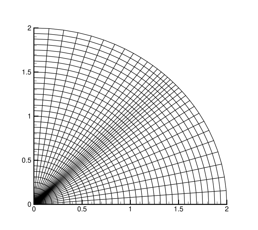
a

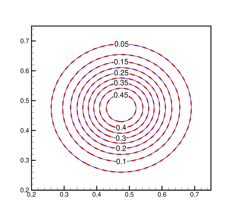
b

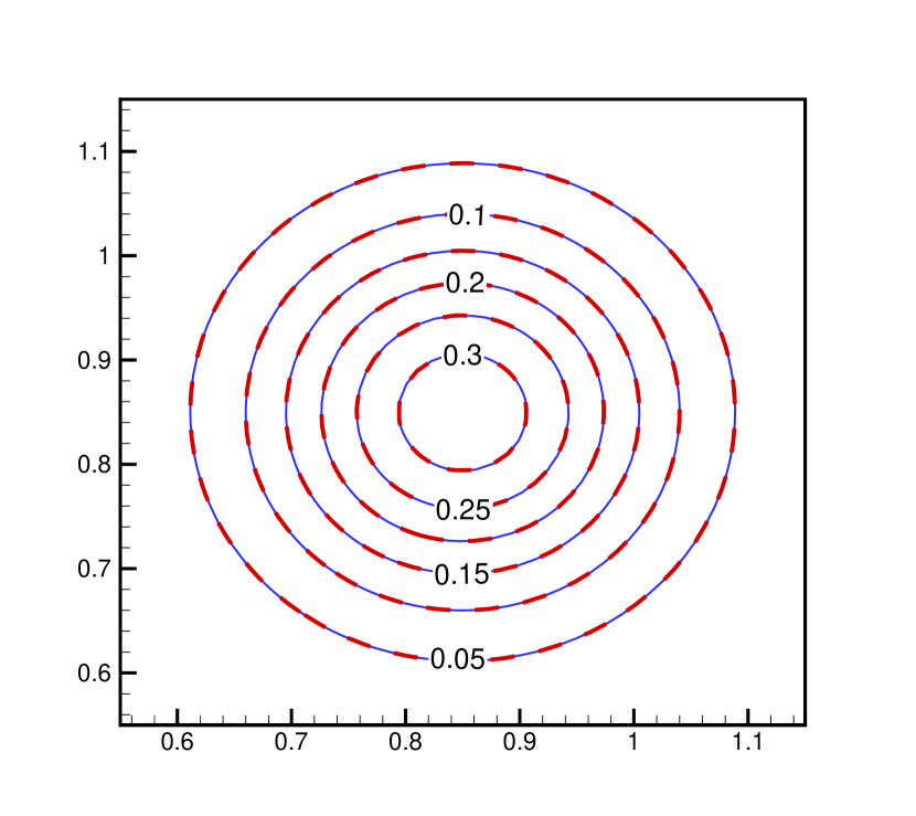
c

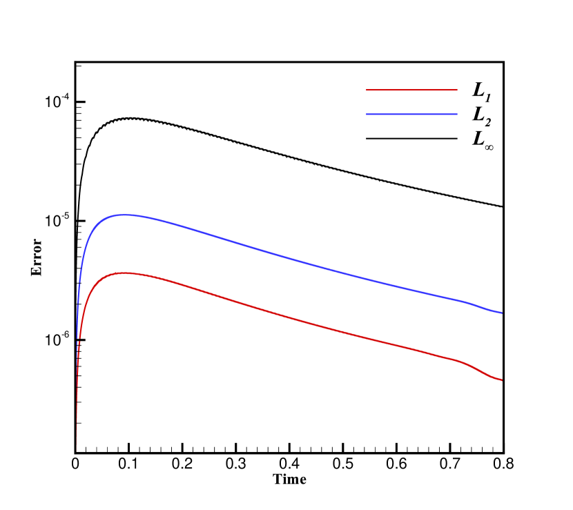
d

Figure 2: Problem 1: (a) Typical $33\times 33$ grids ; exact (red) and numerical (blue) contour plots of the Gaussian pulse at (b) $t$=0.25, (c) $t$=0.50; (d) time evolution of $L_{1}$, $L_{2}$ and $L_{\infty}$ norm errors.

Table 1: Problem 1: $L_{1}$, $L_{2}$ and $L_{\infty}$ norm errors of $\phi$ at different grids and spatial rate of convergence.

Time		$33\times 33$	order	$65\times 65$	order	$129\times 129$
0.25	$L_{1}$	7.337950e-4	4.20	4.000405e-5	4.02	2.458262e-6
	$L_{2}$	2.248532e-3	4.13	1.285689e-4	4.06	7.682233e-6
	$L_{\infty}$	1.353525e-2	3.92	8.922124e-4	4.07	5.329986e-5
0.50	$L_{1}$	3.322361e-4	4.16	1.862575e-5	4.00	1.160263e-6
	$L_{2}$	1.027532e-3	4.10	6.000015e-5	4.04	3.639986e-6
	$L_{\infty}$	6.769672e-3	4.02	4.174938e-4	3.98	2.645134e-5

Table 2: Problem 1: $L_{1}$, $L_{2}$ and $L_{\infty}$ norm errors of $\phi$ at different values of $\delta t$ and temporal rate of convergence.

Time		$\delta t=0.02$	order	$\delta t=0.01$	order	$\delta t=0.005$
0.50	$L_{1}$	1.223078e-3	2.02	3.021393e-4	2.00	7.539567e-5
	$L_{2}$	4.799785e-3	2.01	1.192406e-3	2.00	2.976308e-4
	$L_{\infty}$	4.591702e-2	2.07	1.096137e-2	2.03	2.684967e-3
0.80	$L_{1}$	6.590089e-4	2.10	1.544171e-4	2.03	3.775900e-5
	$L_{2}$	3.082619e-3	2.05	7.453994e-4	2.02	1.837000e-4
	$L_{\infty}$	3.164249e-2	2.06	7.566624e-3	2.03	1.850045e-3

Comparisons between the numerical and exact solutions at two different times $t$=0.25 and $t$=0.50 are presented in figs. 2 and 2 respectively. The numerical solution is seen to be almost indistinguishable from the exact solution conforming to the efficiency of the present scheme to capture the moving pulse accurately. $L_{1}$, $L_{2}$, and $L_{\infty}$ norm errors at each time step for the entire computation time are presented in fig. 2. The similar temporal decaying nature of all three norm errors justifies the convergence of the present scheme.

A quantitative assessment of the numerical solution has been carried out in tables 1 and 2. In table 1, we have calculated the spatial order of convergence for the computation done on three grids of different sizes $33\times 33$, $65\times 65$ and $129\times 129$ with $\delta t$=2.5e-5. For the temporal rate of convergence computations are carried out with $\delta t$=0.02, $\delta t$=0.01 and $\delta t$=0.005 on a $129\times 129$ grid. The clustering parameter has been kept at $\lambda_{\theta}$=0.1 to make spatial error much smaller compared to the temporal error. Computed errors at various times along with the temporal accuracy have been presented in table 2. The scheme shows a near fourth order convergence in space and a temporal accuracy of second order.

4.2 Problem 2: Driven polar cavity

A driven flow inside a polar cavity is also been simulated using the present scheme. This problem is governed by the transient form of N-S equation which can be given as,

$$\omega_{t}=\frac{1}{Re}\left(\omega_{rr}+\frac{1}{r}\omega_{r}+\frac{1}{r^{2}}\omega_{\theta\theta}\right)-\left(u\omega_{r}+\frac{v}{r}\omega_{\theta}\right),$$ (23a)

$$\omega=-\left(\psi_{rr}+\frac{1}{r}\psi_{r}+\frac{1}{r^{2}}\psi_{\theta\theta}\right)$$ (23b)

where $u(r,\theta)=\dfrac{1}{r}\psi_{\theta}$ and $v(r,\theta)=-\psi_{r}$ are the radial and tangential velocity components respectively.

This particular problem was first studied experimentally and numerically by Fuchs and Tillmark [15] and since then it has been used extensively by researchers to validate numerical schemes, particularly for physical domains with circular arc as boundaries [16, 9, 10, 17, 11].

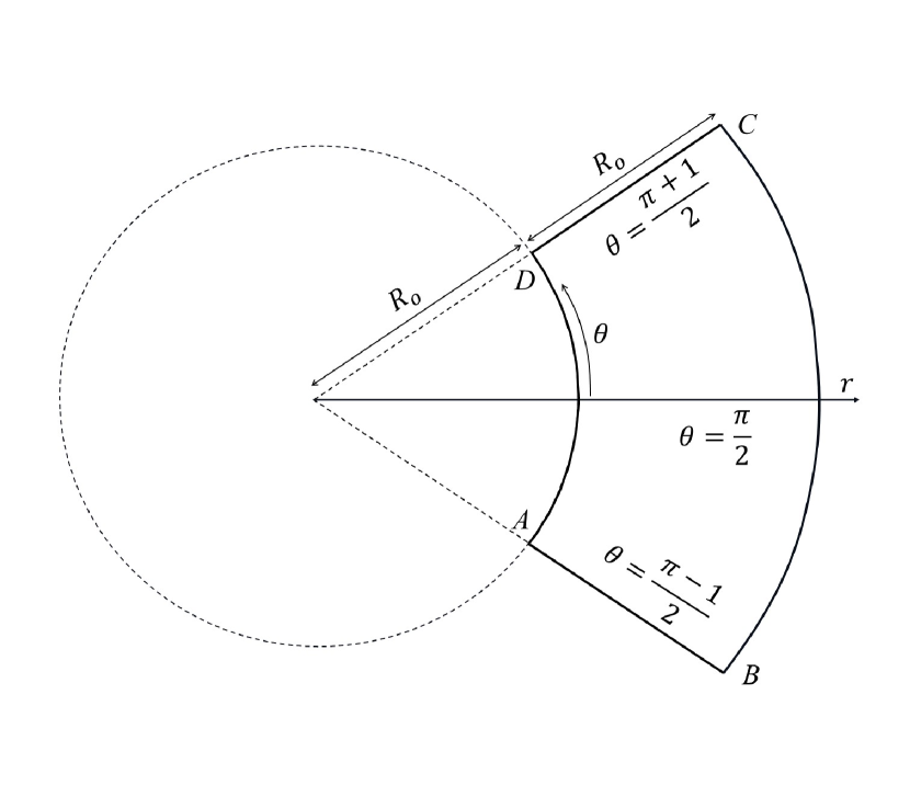
a

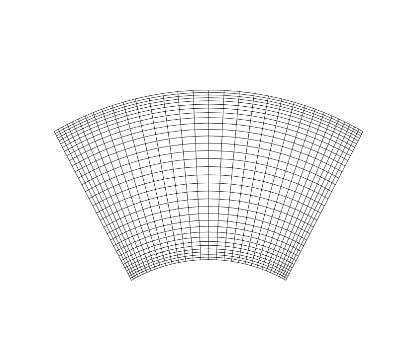
b

Figure 3: Problem 2: (a) Schematic diagram and (b) typical $33\times 33$ centrosymmetric polar grid for flow inside a polar cavity.

The problem is defined in an annular region $\left[1,2\right]\times\left[\dfrac{\pi-1}{2},\dfrac{\pi+1}{2}\right]$. A schematic illustration of the problem is presented in fig. 3. The region $ABCD$ is the domain of the problem: the height $AB=DC$ of the cavity is equal to the radius $R_{0}$=1 of the inner circle. The inner circular arc $DA$ rotates with a unit velocity in the clockwise direction which drives the flow inside the cavity. All the other boundary walls are stationary throughout the simulation. From this, we can derive the boundary conditions for $u$ and $v$ as: $u=0$, $v=-1$ at the moving boundary $DA$ and $u$=0, $v$=0 at all the other boundaries. The streamfunction values are set to be zero at all the boundaries $(\psi=0)$. For this problem, the Reynolds number is defined as $Re=\dfrac{v_{0}R_{0}}{\nu}$, where $v_{0}$ is magnitude of the surface velocity of rotating side $DA$ and $\nu$ is the kinematic viscosity of the fluid. This is imperative to mention here that all boundary walls follow no-slip condition with the fluid inside the cavity, which supplies the following Neumann boundary condition for vorticity.
On the right wall $AB$, $\forall 1\leq i\leq n_{r}$ :

$$\omega_{i,1}=-\frac{2}{r_{i}^{2}h_{\theta_{1}}^{2}}\psi_{i,2}.$$ (24)

On the top wall $BC$, $\forall 1\leq j\leq n_{\theta}$ :

$$\omega_{n_{r},j}=-\frac{2}{h_{r_{n_{r}-1}}^{2}}\psi_{n_{r}-1,j}.$$ (25)

On the left wall $CD$, $\forall 1\leq i\leq n_{r}$ :

$$\omega_{i,n_{\theta}}=-\frac{2}{r_{i}^{2}h_{\theta_{n_{\theta}-1}}^{2}}\psi_{i,n_{\theta}-1}.$$ (26)

On the bottom wall $AB$, $\forall 1\leq j\leq n_{\theta}$ :

$$\omega_{1,j}=-\frac{2}{h_{r_{1}}^{2}}\left(\psi_{2,j}-h_{r_{1}}\right)-\frac{1}{r_{1}}.$$ (27)

After we compute the values of vorticity, the boundary values for its gradients are calculated using one-sided approximations as follows:
On the right wall $AB$, $\forall 1\leq i\leq n_{r}$:

$$\phi_{\theta_{i,1}}=-\frac{h_{\theta_{1}}}{h_{\theta_{2}}(h_{\theta_{1}}+h_{\theta_{2}})}\phi_{i,3}+\frac{h_{\theta_{1}}+h_{\theta_{2}}}{h_{\theta_{1}}h_{\theta_{2}}}\phi_{i,2}-\frac{2h_{\theta_{1}}+h_{\theta_{2}}}{h_{\theta_{1}}(h_{\theta_{1}}+h_{\theta_{2}})}\phi_{i,1}+\mathcal{O}\left(h_{\theta_{2}}(h_{\theta_{1}}+h_{\theta_{2}})^{2}\right).$$ (28)

On the top wall $BC$, $\forall 1\leq j\leq n_{\theta}$:

$$\phi_{r_{n_{r},j}}= \dfrac{h_{r_{n_{r}-1}}}{h_{r_{n_{r}-2}}(h_{r_{n_{r}-1}}+h_{r_{n_{r}-2}})}\phi_{n_{r}-2,j}-\dfrac{h_{r_{n_{r}-1}}+h_{r_{n_{r}-2}}}{h_{r_{n_{r}-1}}h_{r_{n_{r}-2}}}\phi_{n_{r}-1,j}$$ (29)

$$+\dfrac{2h_{r_{n_{r}-1}}+h_{r_{n_{r}-2}}}{h_{r_{n_{r}-1}}(h_{r_{n_{r}-1}}+h_{r_{n_{r}-2}})}\phi_{n_{r},j}+\mathcal{O}\left(h_{r_{n_{r}-1}}(h_{r_{n_{r}-1}}+h_{r_{n_{r}-2}})^{2}\right).$$

On the left wall $CD$, $\forall 1\leq i\leq n_{r}$:

$$\phi_{\theta_{i,n_{\theta}}}= \frac{h_{\theta_{n_{\theta}-1}}}{h_{\theta_{n_{\theta}-2}}(h_{\theta_{n_{\theta}-1}}+h_{\theta_{n_{\theta}-2}})}\phi_{i,n_{\theta}-2}-\frac{h_{\theta_{n_{\theta}-1}}+h_{\theta_{n_{\theta}-2}}}{h_{\theta_{n_{\theta}-1}}h_{\theta_{n_{\theta}-2}}}\phi_{i,n_{\theta}-1}$$ (30)

$$+\frac{2h_{\theta_{n_{\theta}-1}}+h_{\theta_{n_{\theta}-2}}}{h_{\theta_{n_{\theta}-1}}(h_{\theta_{n_{\theta}-1}}+h_{\theta_{n_{\theta}-2}})}\phi_{i,n_{\theta}}+\mathcal{O}\left(h_{\theta_{n_{\theta}-1}}(h_{\theta_{n_{\theta}-1}}+h_{\theta_{n_{\theta}-2}})^{2}\right).$$

On the bottom wall $DA$, $\forall 1\leq j\leq n_{\theta}$:

$$\phi_{r_{1,j}}=-\frac{h_{r_{1}}}{h_{r_{2}}(h_{r_{1}}+h_{r_{2}})}\phi_{3,j}+\frac{h_{r_{1}}+h_{r_{2}}}{h_{r_{1}}h_{r_{2}}}\phi_{2,j}-\frac{2h_{r_{1}}+h_{r_{2}}}{h_{r_{1}}(h_{r_{1}}+h_{r_{2}})}\phi_{1,j}+\mathcal{O}\left(h_{r_{2}}(h_{r_{1}}+h_{r_{2}})^{2}\right).$$ (31)

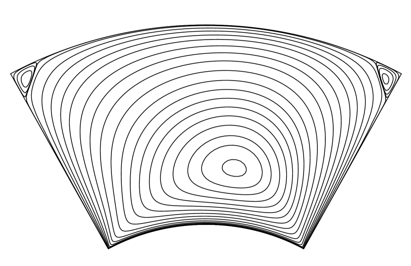
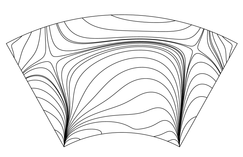
a

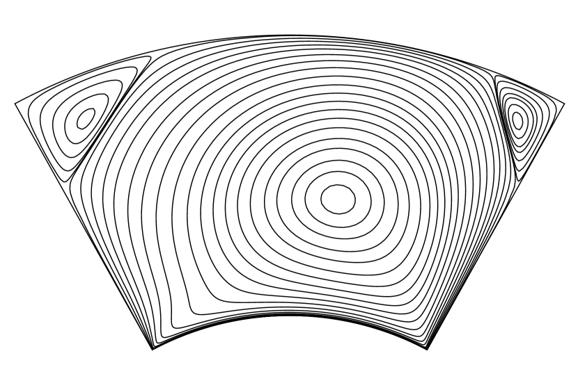
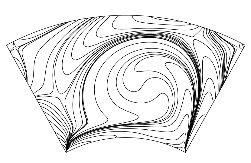
b

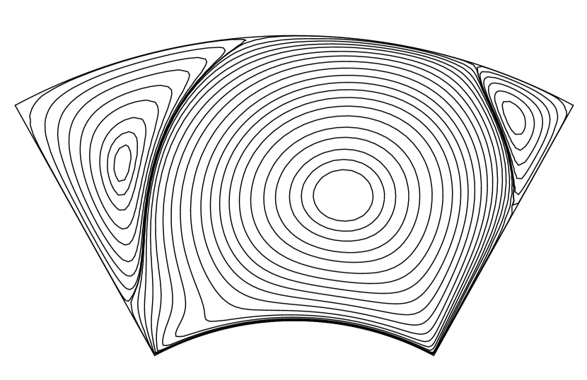
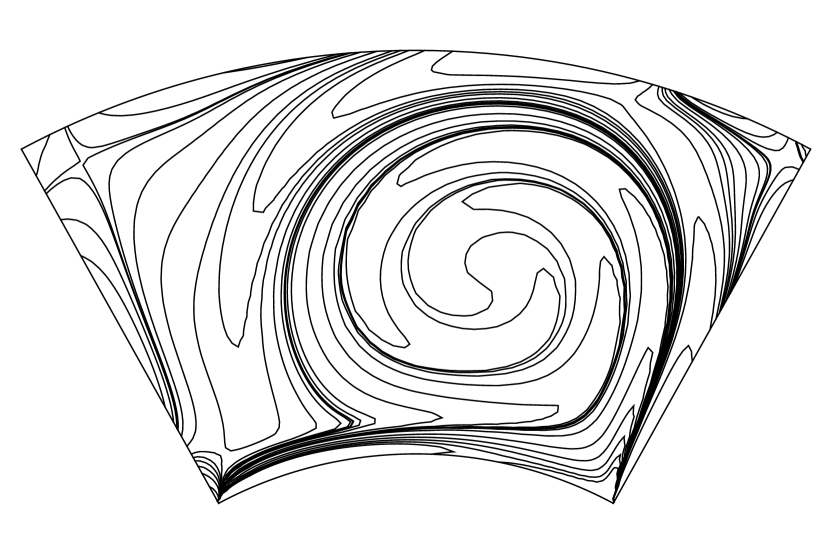
c

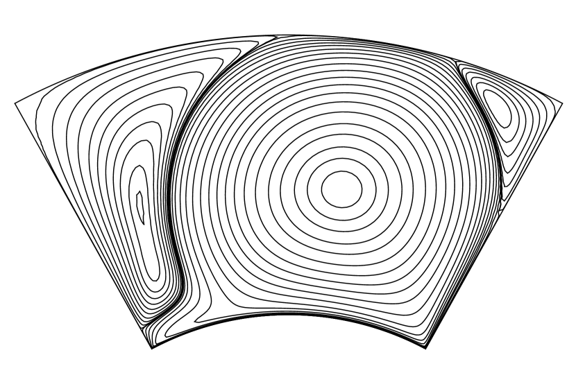
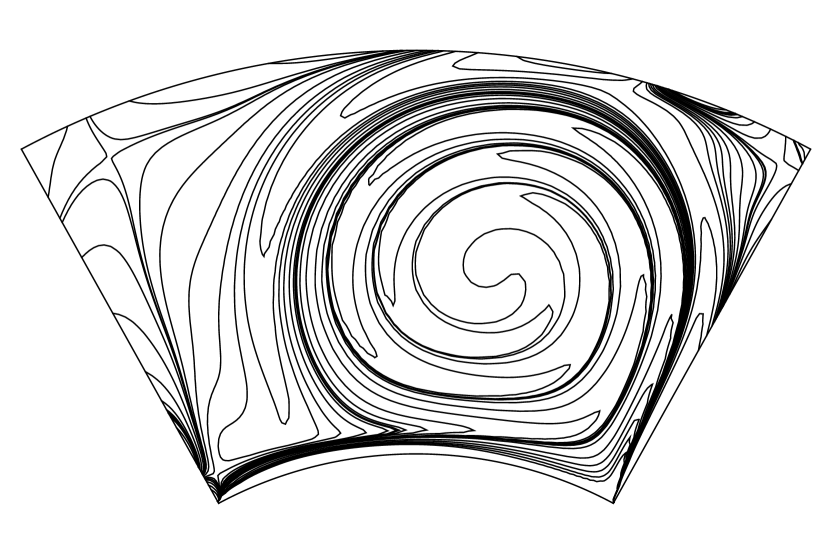
d

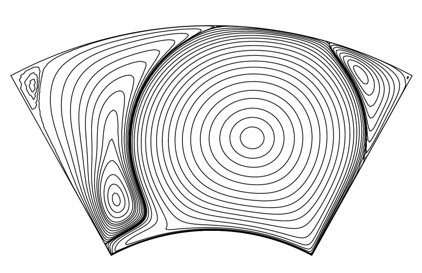
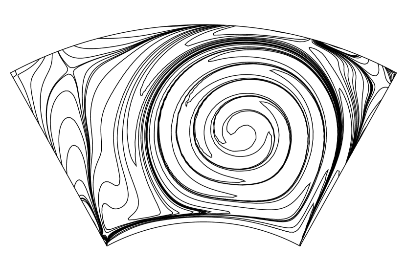
e

Figure 4: Problem 2: Contours of streamfunction (left) and vorticity (right) computed with $65\times 65$ grids: (a)$Re=55$, (b)$Re=350$, (c)$Re=1000$, (d)$Re=2000$ and (e)$Re=3000$.

While working with this problem, Lee and Tsuei [16] witnessed that large solution errors propagate near the rotating boundary. Besides, vortices are also created at the solid boundaries of the cavity. Therefore it is necessary to introduce a maximum number of grids in the vicinity of cavity walls as can be seen in fig. 3. This has been achieved using modified versions of the grid-generating function

$$r_{i}=L_{r}\left\{\frac{i}{n_{r}}+\frac{\lambda_{r}}{\Theta_{r}}\sin{\left(\frac{i\Theta_{r}}{n_{r}}\right)}\right\}.$$ (32)

along with equation 22 with proper choices of the constants $L_{r}=L_{\theta}=1.0$, $\lambda_{r}=\lambda_{\theta}=-0.55$ and $\Theta_{r}=\Theta_{\theta}=2\pi$.

The computations for this problem are carried out for Reynolds numbers 55, 350, 1000, 2000, 3000 and 5000. The post processed steady-state streamfunction $(\psi)$ and vorticity $(\omega)$ contours for $55\leq Re\leq 3000$ are plotted in fig. 4. As $Re$ increases the primary vortex is seen to move gradually towards the right wall of the cavity. Similar to the case of flow inside a square cavity, with an increase in the value of $Re$ the secondary vortices at the corners opposite to the moving wall grow in size, particularly the secondary left vortex gains significantly more size as compared to the secondary right vortex and for higher values of $Re$ the former tends to occupy the entire left side of the cavity. Further, at $Re$=3000 a tertiary vortex is seen to form at the top left corner of the cavity. It is to be mentioned that all the findings are in accordance with those available in the literature [16, 9, 10, 17, 11] both experimentally and numerically. Additionally, at higher $Re$ values the vorticity contours move away from the center of the cavity toward the cavity walls thereby developing very strong vorticity gradients in the vicinity of the cavity walls.

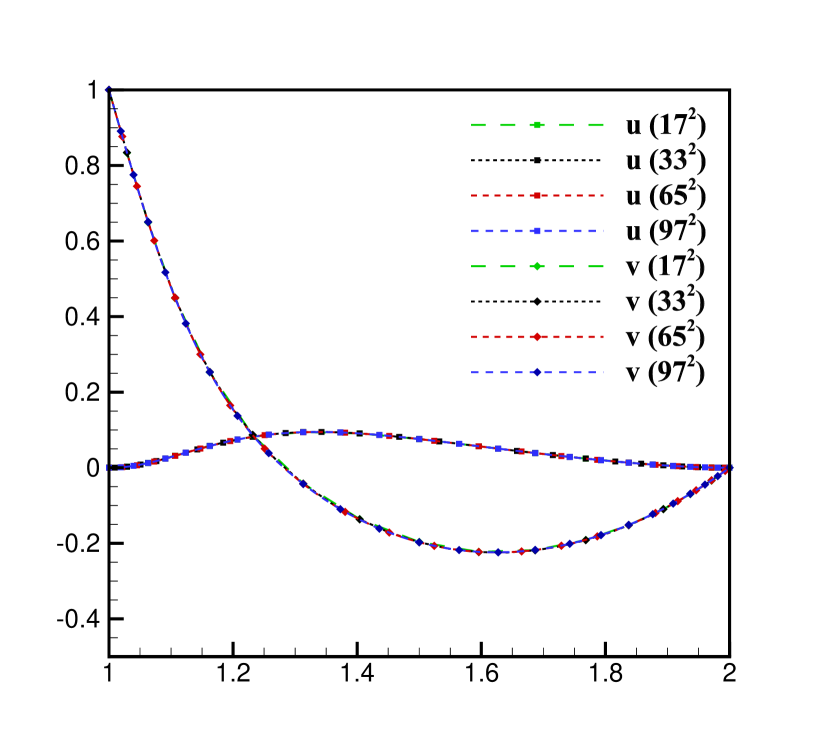
a

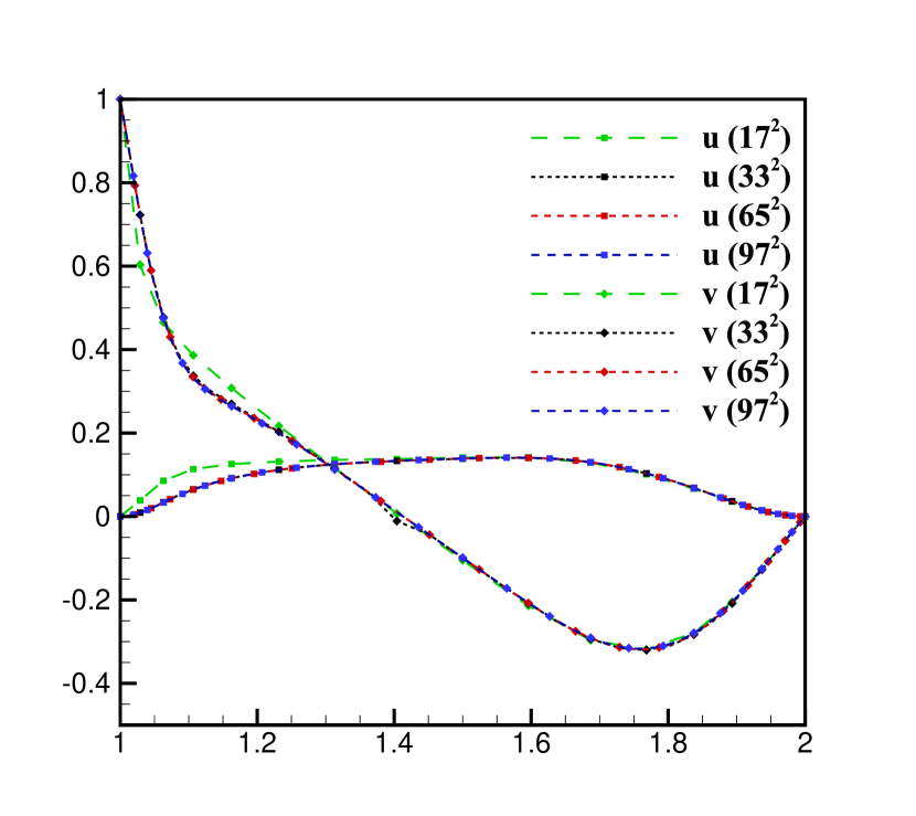
b

Figure 5: Problem 2: The $u$- and $v$-velocity profiles along $\theta=\dfrac{\pi}{2}$ computed on grids of different sizes for (a)$Re=55$ and (b)$Re=350$.

Fig. 5 presents the $u$ and $v$ velocity profiles along the radial line $\theta=\dfrac{\pi}{2}$ computed on grids of four different sizes $17\times 17$, $33\times 33$, $65\times 65$ and $97\times 97$ for $Re$’s $55$ and $350$. These figures show that the computed results are unaffected by the change in grid points and a $65\times 65$ grid is sufficient to achieve a grid-independent solution for both values of the Reynolds number.

For this problem, we have also computed the perceived rate of convergence [18]. Despite best efforts, we could not trace the estimation of perceived order in nonuniform polar grid. The increased flow complexity in case of higher $Re$ value makes the estimation of rate of convergence computation extensive [18]. Therefore the perceived order of convergence has been computed only for the cases $Re$=55 and 350. We employ grids of three different sizes viz. $33\times 33$, $65\times 65$ and $97\times 97$ and compute with $\delta t$=1e-4 to minimize temporal error. The perceived order of convergence for streamfunction has been estimated in table 3 whereas convergence of vorticity is compiled in table 4. From these tables, we can observe that the order of convergence for vorticity, in $L_{2}$-norm error, drops below quadratic because of increased flow complexity. Moreover, it is amply clear that the mesh $97\times 97$ should be ideally suited to compute in conjunction with the present discretization strategy.

Table 3: Problem 2: $L_{1}$ and $L_{2}$ norm difference in streamfunction and perceived order of convergence in space.

$Re$	Grid size	$L_{1}-$norm	order	$L_{2}-$norm	order
55	$33^{2}$
		$\left\|\psi_{2}-\psi_{1}\right\|$=4.829202e-5		$\left\|\psi_{2}-\psi_{1}\right\|$=7.723404e-5
	$65^{2}$		3.17		2.64
		$\left\|\psi_{3}-\psi_{1}\right\|$=6.470839e-5		$\left\|\psi_{3}-\psi_{1}\right\|$=1.039171e-4
	$97^{2}$
350	$33^{2}$
		$\left\|\psi_{2}-\psi_{1}\right\|$=1.710546e-4		$\left\|\psi_{2}-\psi_{1}\right\|$=2.594515e-4
	$65^{2}$		2.61		2.41
		$\left\|\psi_{3}-\psi_{1}\right\|$=2.469988e-4		$\left\|\psi_{3}-\psi_{1}\right\|$=3.867575e-4
	$97^{2}$

Table 4: Problem 2: $L_{1}$ and $L_{2}$ norm difference in vorticity and perceived order of convergence in space.

$Re$	Grid size	$L_{1}-$norm	order	$L_{2}-$norm	order
55	$33^{2}$
		$\left\|\omega_{2}-\omega_{1}\right\|$=3.057162e-1		$\left\|\omega_{2}-\omega_{1}\right\|$=2.983460e0
	$35^{2}$		2.26		1.52
		$\left\|\omega_{3}-\omega_{1}\right\|$=4.672710e-1		$\left\|\omega_{3}-\omega_{1}\right\|$=5.259851e0
	$97^{2}$
350	$33^{2}$
		$\left\|\omega_{2}-\omega_{1}\right\|$=3.919087e-1		$\left\|\omega_{2}-\omega_{1}\right\|$=3.232429e0
	$65^{2}$		2.52		1.66
		$\left\|\omega_{3}-\omega_{1}\right\|$=5.739092e-1		$\left\|\omega_{3}-\omega_{1}\right\|$=5.534059e0
	$97^{2}$

Next, we carry out a qualitative comparison of the numerically attained results for $Re=55$ and $350$ with those of the experimental findings reported by Fuchs and Tillmark [15]. In fig. 6 we present the numerically simulated steady-state streamlines for $Re=55$ and $350$ along with those of the experimental ones. Moreover, the numerically obtained $u$ and $v$ velocity profiles along the radial line $\theta=\dfrac{\pi}{2}$ are compared to those of [15] in fig. 7. Both numerical and experimental solutions show good agreement with each other for each $Re$ value. The $u$ and $v$ velocity profiles along $\theta=\dfrac{\pi}{2}$ for $Re$ values 1000, 2000, and 3000 are presented in fig. 8, though there is no quantitative evidence available for the same in the literature. Additionally, the variation of the vorticity along the rotating wall and the radial line $\theta=\dfrac{\pi}{2}$ are depicted in fig. 9. It can be seen that both the radial and tangential velocities become stronger in the vicinity of the circular walls of the cavity, whereas the vorticity gradients can be seen to develop near all the boundary walls at higher values of Reynolds numbers. These observations are in line with those reported in [10]. In tables 5 and 6 we compile all our quantitative data pertaining to the primary and secondary vortices. Tables 5 and 6 also carry out a comparison of strength and location of the vortices with those available in the literature for $55\leq Re\leq 3000$. It is heartening to notice that our computation compares well with the firmly established studies available in the literature.

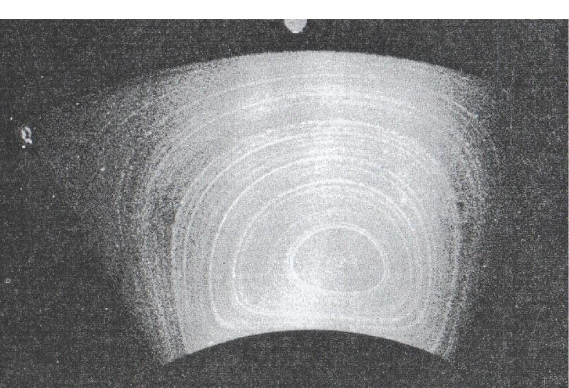
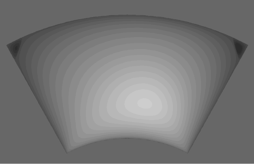
a

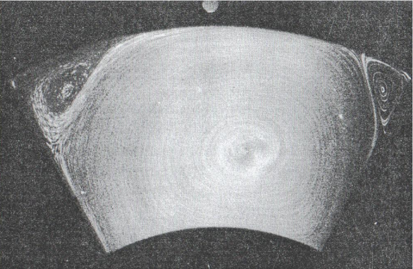
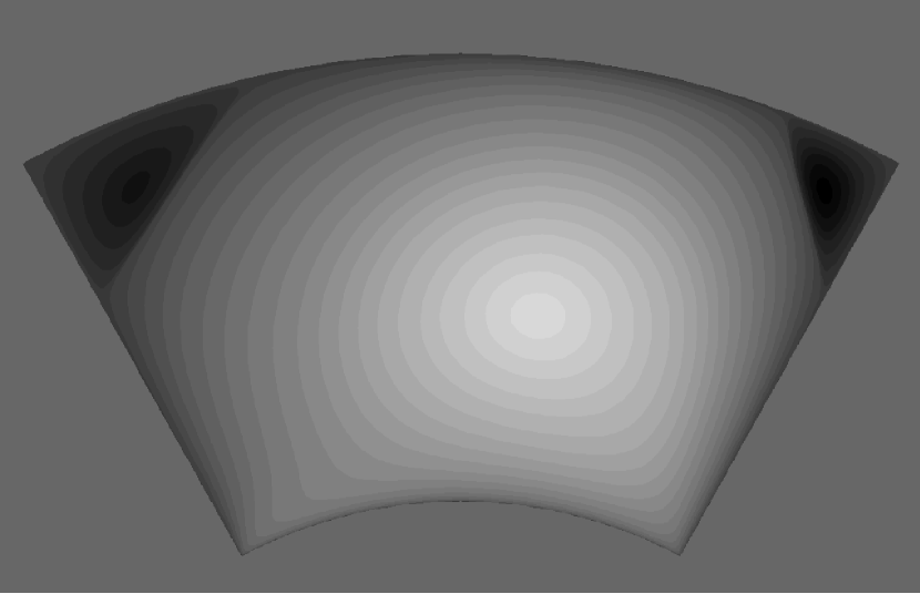
b

Figure 6: Problem 2: Comparison of experimental [15] (left) and numerical (right) steady-state streamfunction contours of driven polar cavity problem for (a) $Re=55$ and (b) $Re=350$.

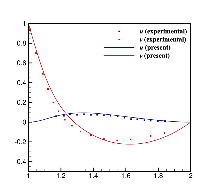
a

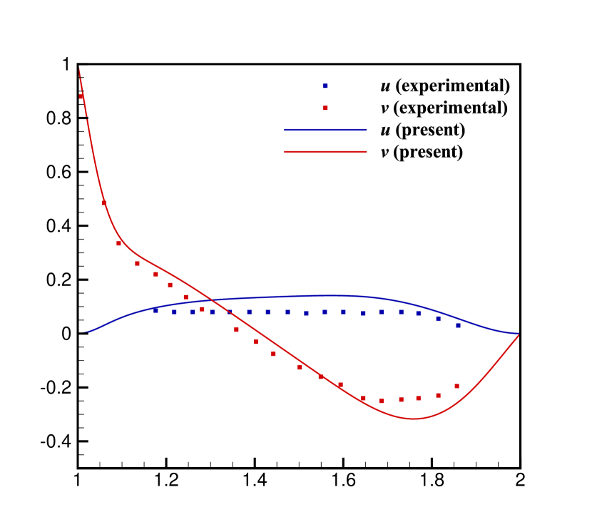
b

Figure 7: Problem 2: Comparisons of steady-state $u$- and $v$-velocity profiles along the radial line $\theta=\frac{\pi}{2}$ with [15] for (a) $Re=55$ and (b) $Re=350$.

a

b

Figure 8: Problem 2: Steady-state (a) $u$- and (b) $v$-velocity profiles along the radial line $\theta=\dfrac{\pi}{2}$ for different $Re$ values.

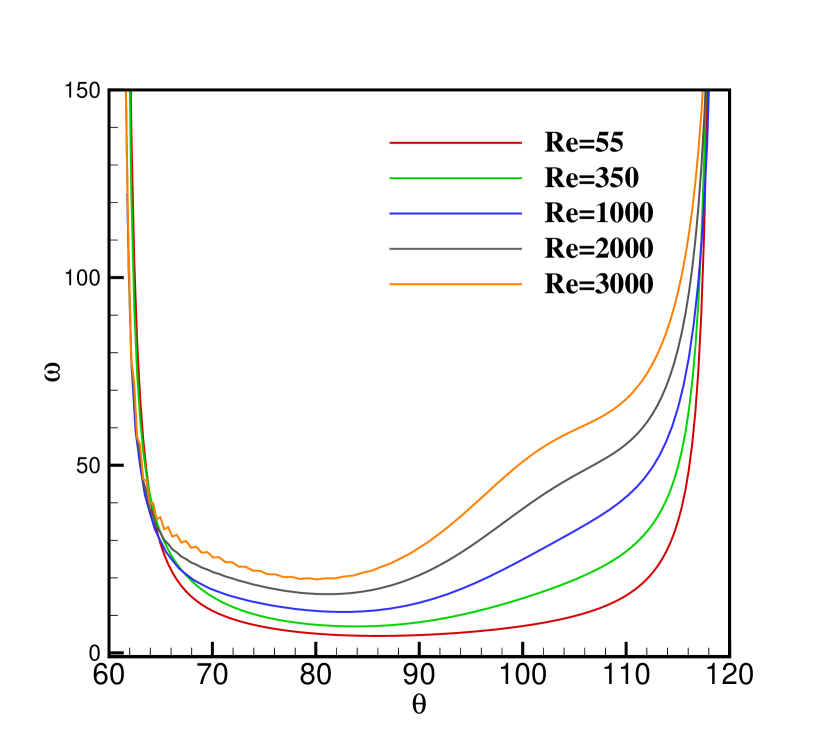
a

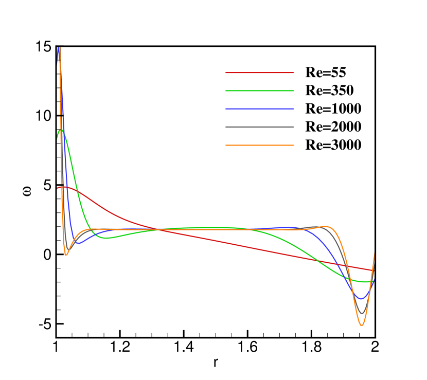
b

Figure 9: Problem 2: Vorticity contours for different $Re$ values along (a) the rotating wall and (b) the radial line $\theta=\dfrac{\pi}{2}$.

Table 5: Problem 2: Strength and location of the centre of primary vortex for different Reynolds numbers.

$Re$		Grid Size	$\psi_{max}$	$x$	$y$
55	[10]	$513\times 513$	0.1155	0.141	1.281
	[17]	$83\times 119$	0.1155	0.138	1.285
	[11]	$81\times 81$	0.1156	0.142	1.285
	Present	$65\times 65$	0.1153	0.143	1.282
350	[10]	$513\times 513$	0.1263	0.167	1.414
	[17]	$83\times 119$	0.1263	0.163	1.411
	[11]	$81\times 81$	0.1266	0.171	1.414
	Present	$65\times 65$	0.1243	0.158	1.411
1000	[10]	$513\times 513$	0.1275	0.169	1.439
	[17]	$83\times 119$	0.1275	0.166	1.436
	[11]	$81\times 81$	0.1275	0.174	1.444
	Present	$65\times 65$	0.1270	0.167	1.448
2000	[10]	$513\times 513$	0.1253	0.188	1.447
	Present	$97\times 97$	0.1250	0.194	1.447
3000	[17]	$109\times 157$	0.1240	0.196	1.447
	Present	$97\times 97$	0.1237	0.194	1.447

Table 6: Problem 2: Strength and location of the centre of secondary vortices for different Reynolds numbers.

		Secondary Right				Secondary Left
$Re$		$\psi_{min}$	$x$	$y$		$\psi_{min}$	$x$	$y$
55	[10]	-8.690e-6	0.881	1.730		-4.690e-6	-0.880	1.729
	[17]	-7.964e-6	0.883	1.731		-4.994e-6	-0.876	1.742
	[11]	-8.102e-6	0.882	1.735		-4.391e-6	-0.882	1.735
	Present	-9.602e-6	0.879	1.726		-5.140e-6	-0.879	1.726
350	[10]	-5.490e-4	0.794	1.697		-3.990e-4	-0.702	1.695
	[17]	-5.469e-4	0.796	1.690		-4.009e-4	-0.696	1.699
	[11]	-5.435e-4	0.796	1.689		-4.010e-4	-0.701	1.703
	present	-5.525e-4	0.790	1.692		-3.388e-4	-0.704	1.697
1000	[10]	-2.120e-3	0.757	1.713		-3.460e-3	-0.590	1.552
	[17]	-2.099e-3	0.755	1.717		-3.480e-3	-0.589	1.549
	[11]	-2.106e-3	0.762	1.705		-3.488e-3	-0.592	1.559
	Present	-2.238e-3	0.749	1.729		-3.446e-3	-0.599	1.537
2000	[10]	-3.080e-3	0.734	1.743		-4.830e-3	-0.522	1.406
	Present	-3.151e-3	0.734	1.734		-4.835e-3	-0.519	1.393
3000	[17]	-3.325e-3	0.724	1.757		-7.089e-3	-0.459	1.156
	Present	-3.559e-3	0.714	1.770		-7.062e-3	-0.452	1.149

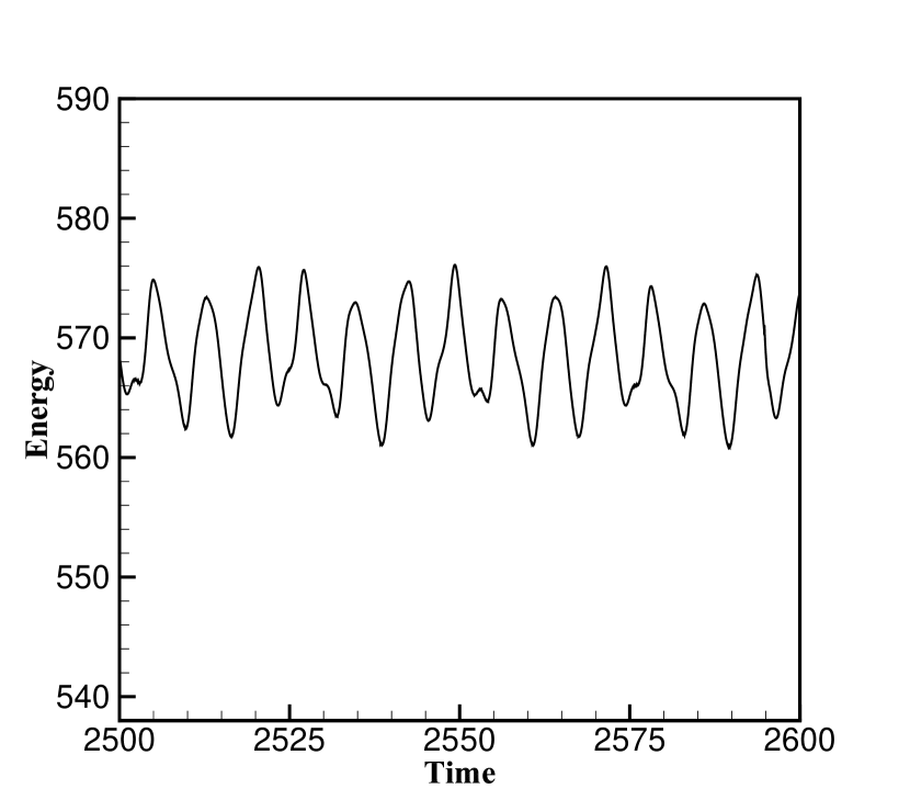
a

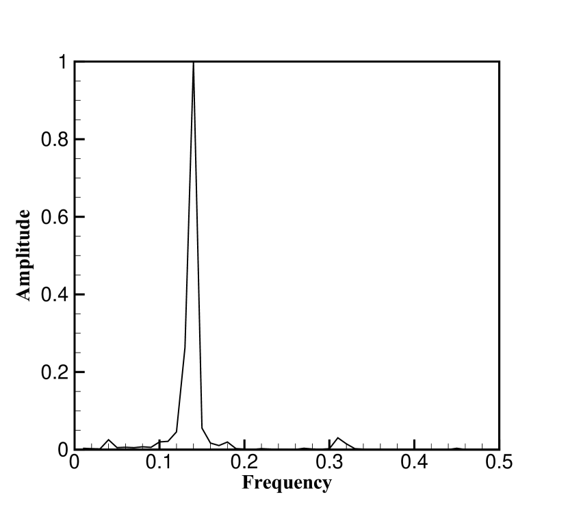
b

Figure 10: Problem 2: (a) Time history and (b) power spectrum of total energy of the flow inside a polar cavity for $Re=5000$.

Subsequently, we carry out our computation for $Re=5000$ on a $129\times 129$ nonuniform polar grid. To the best of the authors knowledge, the solution to this problem for Reynolds numbers as high as 5000 has not been computed using a transient scheme. Sen and Kalita [17] in their work used a steady code to arrive at a converged solution at $Re=5000$. Also authors used a $82\times 118$ grid with exponential clustering at the inner wall along the radial direction. In this work we intend to better capture the physics of the flow and hence use appropriately clustering on all boundaries. It is interesting to notice that the present discretization of the N-S equation shows a gradual convergence towards a stable periodic solution rather than a steady-state solution as reported in [17]. Time evolution of the physical property of the flow inside the cavity helps to establish the periodic nature of the solution. Temporal progression of the total energy inside the cavity is presented in fig. 10. We perform the spectral density analysis for the variation of energy which results in a single frequency peak as can be seen in fig. 10. This further ascertains the periodicity of the flow. Nevertheless, accurate estimation of the frequency and time-period of the solution leaves further scope of investigation of this problem.

4.3 Problem 3: Natural convection in horizontal concentric annulus

We further analyze the efficiency of the newly developed scheme to tackle heat transfer by implementing it to solve natural heat convection inside a horizontal concentric annulus. This problem has gained a considerable amount of attention from researchers over the years because of its relevance and applicability in various engineering and physical situations, such as heat exchangers, solar collectors, nuclear reactors, thermal energy storage systems, etc [19, 20, 21, 22, 23, 24, 25, 26, 27]. It is governed by the transient Boussinesq equations which in the polar coordinate system are given as,

$$\omega_{t}=Pr\left(\omega_{rr}+\frac{1}{r}\omega_{r}+\frac{1}{r^{2}}\omega_{\theta\theta}\right)-\left(u\omega_{r}+\frac{v}{r}\omega_{\theta}\right)+RaPr\left(\mathcal{T}_{r}\cos{\theta}-\mathcal{T}_{\theta}\frac{\sin{\theta}}{r}\right),$$ (33a)

$$\omega=-\left(\psi_{rr}+\frac{1}{r}\psi_{r}+\frac{1}{r^{2}}\psi_{\theta\theta}\right),$$ (33b)

$$\mathcal{T}_{t}=\left(\mathcal{T}_{rr}+\frac{1}{r}\mathcal{T}_{r}+\frac{1}{r^{2}}\mathcal{T}_{\theta\theta}\right)-\left(u\mathcal{T}_{r}+\frac{v}{r}\mathcal{T}_{\theta}\right).$$ (33c)

where $\mathcal{T}$ denotes the dimensionless temperature, $Pr$ and $Ra$ stand for Prandtl number and Rayleigh number respectively. The Rayleigh number $Ra$ is a dimensionless quantity defined as $Ra=\dfrac{g\beta\delta\mathcal{T}L^{3}}{\kappa\nu}$, where $g$ is the acceleration due to gravity, $\beta$ is the coefficient of thermal expansion of the fluid, $\delta\mathcal{T}$ is the temperature difference, $L$ is the length, $\kappa$ is the thermal diffusivity and $\nu$ is the kinematic viscosity of the fluid.

a

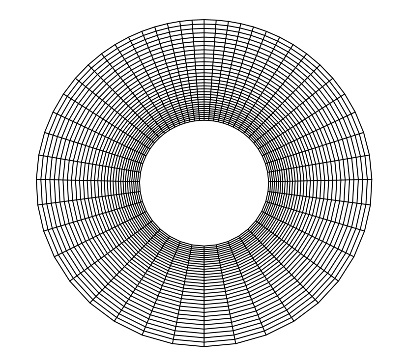
b

Figure 11: Problem 3: (a) Problem setup and (b) typical noununiiform polar grid for heat transfer in horizontal annulus.

The problem setup consists of two concentric circular walls of which the inner circle has a radius $R_{i}$ and the outer circle has a radius $R_{o}$. Two different temperatures are maintained at the inner and outer circular walls of the annulus as shown in fig. 11. The simulation is carried out for $Ra$ values 2.38e3, 9.50e3, 4.70e4, 6.19e4, and 1.02e5. The values of the $Pr$ is set as 0.706, 0.717, and 0.718. For each case, we have considered $L/D_{i}$=0.8, where $L=R_{o}-R_{i}$ and $D_{i}=2\texttimes R_{i}$. The inner wall is heated to a unit nondimensional temperature $(\mathcal{T}_{h}=1)$ keeping the outer wall’s temperature at zero $(\mathcal{T}_{c}=0)$. This temperature difference serves as the driving force for the flow in this simulation. The values of streamfunction and vorticity at the inner and outer boundaries of the annulus are obtained respectively from no-slip criteria between the fluid and the walls of the annulus and one-sided approximations introduced in equations 28, 29, 30 and 31. The prior studies help us to identify that the near boundary region of the inner circle and the radial line $\theta=\dfrac{\pi}{2}$ should be observed cautiously. This motivates us to work with a mesh where grid points are clustered in these regions (see fig. 11). The grid is generated by making adequate changes in equations 32 and 22 and choosing the associated parameters as $L_{r}=0.8$, $L_{\theta}=2\pi$, $\Theta_{r}=\pi$, $\Theta_{\theta}=2\pi$, $\lambda_{r}=-0.4$ and $\lambda_{\theta}=0.25$.

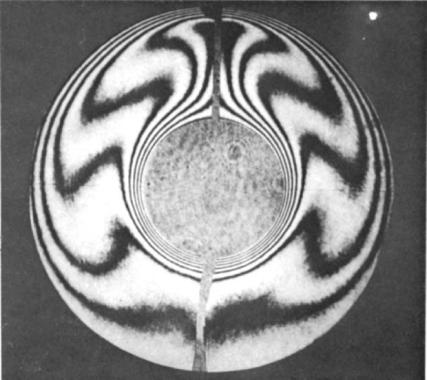
a

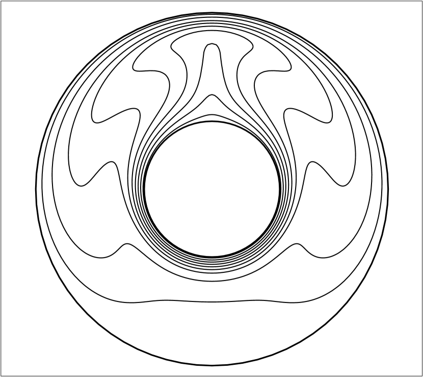
b

Figure 12: Problem 3: Steady-state isotherms at $Ra=4.7e4$, $Pr$=0.706: (a) experimental solution [21] and (b) numerical solution.

The numerical results of the present simulation have been presented in figs. 12 and 13. We carry out a qualitative comparison in fig. 12 where the numerically obtained steady-state isotherm contours for $Ra=4.7e4$, $Pr$=0.706 are depicted alongside that of the experimental study [21]. The figure shows that the fluid near the hot inner wall of the annulus flows up along the inner boundary and a strong plume emerges above the inner boundary at $\theta=\dfrac{\pi}{2}$, while the fluid near the cold outer wall flows down to the bottom of the annuli as an effect of buoyancy caused by the temperature difference. Once the flow reaches a steady state, the temperature field becomes symmetric. The maximum temperature gradient appears in the raised plume. Good agreements are obtained between the experimental and numerical solutions. Fig. 13 contains the steady-state isotherms alongside the streamfunctions for different $Ra$ values. The figure shows that for lower $Ra$ values natural convection is dominated by heat conduction. Almost concentric isotherms can be seen for $Ra=2.38e3$ while two symmetric vortices can be seen caused by the weak natural convection. As the value of $Ra$ increases the fluid motion driven by buoyancy force also increases, leading to a stronger convection. As a result, the isotherms start moving upward and change shape to form a plume. The plume becomes more prominent with a further increase in the $Ra$ value.

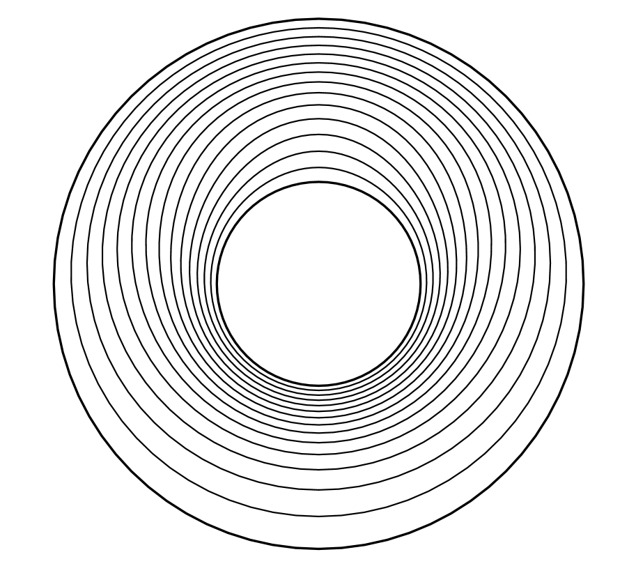
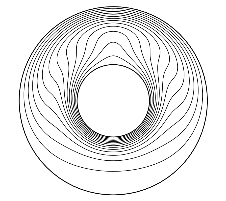
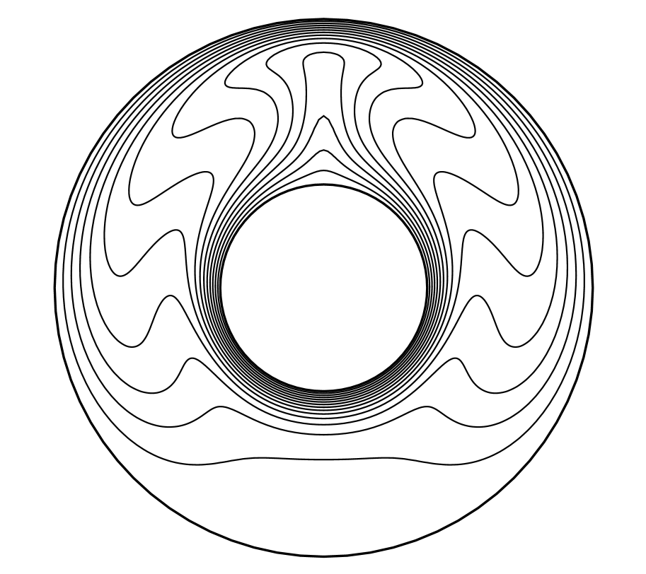
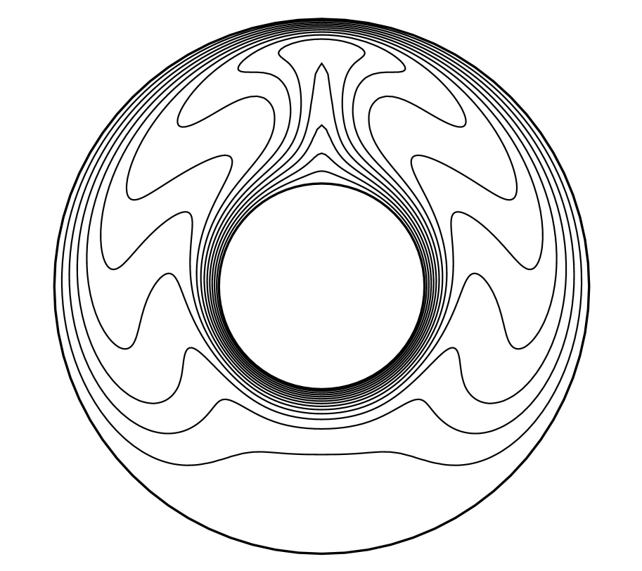
Figure 13: Problem 3: Steady-state isotherms and streamlines for $Ra$ values (a) 2.38e3, (b) 9.50e4, (c) 6.19e4 and (d) 1.02e5.

Additionally, for this problem we have also evaluated the average Nusselt number $(\mkern 1.5mu\overline{\mkern-1.5muNu\mkern-1.5mu}\mkern 1.5mu)$ which is the arithmetic mean of the surface-averaged Nusselt numbers of the annulus walls that are defined as,

$$Nu_{i}=-\frac{1}{\pi}R_{i}\int_{-\frac{\pi}{2}}^{\frac{\pi}{2}}\left.\frac{\partial\mathcal{T}}{\partial r}\right|_{r=R_{i}}d\theta$$ (34)

and

$$Nu_{o}=-\frac{1}{\pi}R_{o}\int_{-\frac{\pi}{2}}^{\frac{\pi}{2}}\left.\frac{\partial\mathcal{T}}{\partial r}\right|_{r=R_{o}}d\theta.$$ (35)

The average Nusselt number thus obtained is compared to the existing studied in table 7. Our computed values agree well with those available in the literature at $Ra$=2.38e3, $Pr$=0.716. But it seen to differ by about 10% as $Ra$ is increased.

Table 7: Problem 3: Comparison of average nusselt number $(\mkern 1.5mu\overline{\mkern-1.5muNu\mkern-1.5mu}\mkern 1.5mu)$ computed using different schemes for different Rayleigh numbers.

$Ra$	$Pr$	[21](expt.)	[24]	[25]	Present
2.38e3	0.716	1.38		1.320	1.3882
9.50e3	0.717	2.01	1.9901	1.999	1.6909
6.19e4	0.718	3.32	3.3092	3.361	2.9176
1.02e5	0.718	3.66	3.6475	3.531	3.2994

4.4 Problem 4: Forced convection over a stationary heated circular cylinder

Finally, we carry out numerical simulation for the classical problem of heat transfer in the fluid flow over the stationary heated circular cylinder. The stationary heated circular cylinder is presumed to be of unit radius ($R_{0}=1$) and immersed in a fluid of infinite domain maintained at unit nondimensional temperature [28, 29, 30, 31, 8, 32, 33, 34, 35, 17, 36, 37, 38]. The cylinder is kept in a cross-flow having uniform velocity $u=U_{\infty}=1$. The 2D flow configuration of the problem is shown in fig. 14a. The cylinder is placed at the center of the circular domain. Following [39], we have set the far field boundary at a distance $R_{\infty}=45R_{0}$. On the solid surface $r=R_{0}$, the boundary conditions for velocity components are those of no-slip conditions, i.e. $u=v=0\implies\psi=0$. In the far stream $r=R_{\infty}$ in front of the cylinder the potential flow is prescribed a unit value $u=U_{\infty}$=1. For this problem, where the simulation results in periodic vortex shedding, at the downstream of the flow, we have imposed the convective boundary conditions $\phi_{t}+U_{\infty}\phi_{r}$=0 (where $\phi$ represents $\psi$, $u$ or $v$) to capture the shedding process efficiently. The continuous shedding of vortices, when they leave the computational domain in the direction of the flow, can be best facilitated by the convective boundary conditions [40, 41, 42, 43]. In addition, at the far field vorticity value decays and becomes $\omega=0$. However, it possesses nonzero value at the inner boundary, which may be derived by making use of the fact that $\psi=0$, $\psi_{r}=0$ on $r=R_{0}$ in equation 33b. The vorticity gradients at all the boundaries are computed using one-sided approximations.

a

Figure 14: Problem 4: (a)Flow configuration and (b) typical $65\times 97$ nonuniform grid.

b

The essential nondimensional parameters for this problem include the Reynolds number ($Re$) and the Prandtl number ($Pr$). In this present investigation, the Prandtl number is fixed at $Pr$=0.7 for all the values of $Re$ under consideration. As shown in fig. 14a, the computational domain is discretized using a nonuniform grid of size $129\times 193$ for all the combinations of $Pr$ and $Re$. With the circular cylinder placed at the center of the domain, grid is clustered in the vicinity of the cylinder wall.

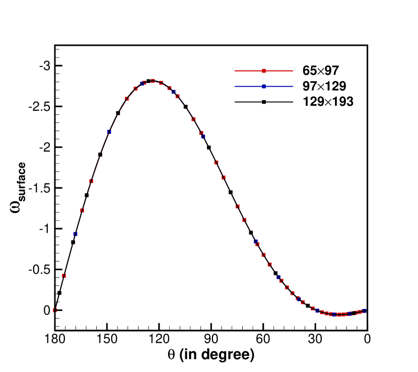
a

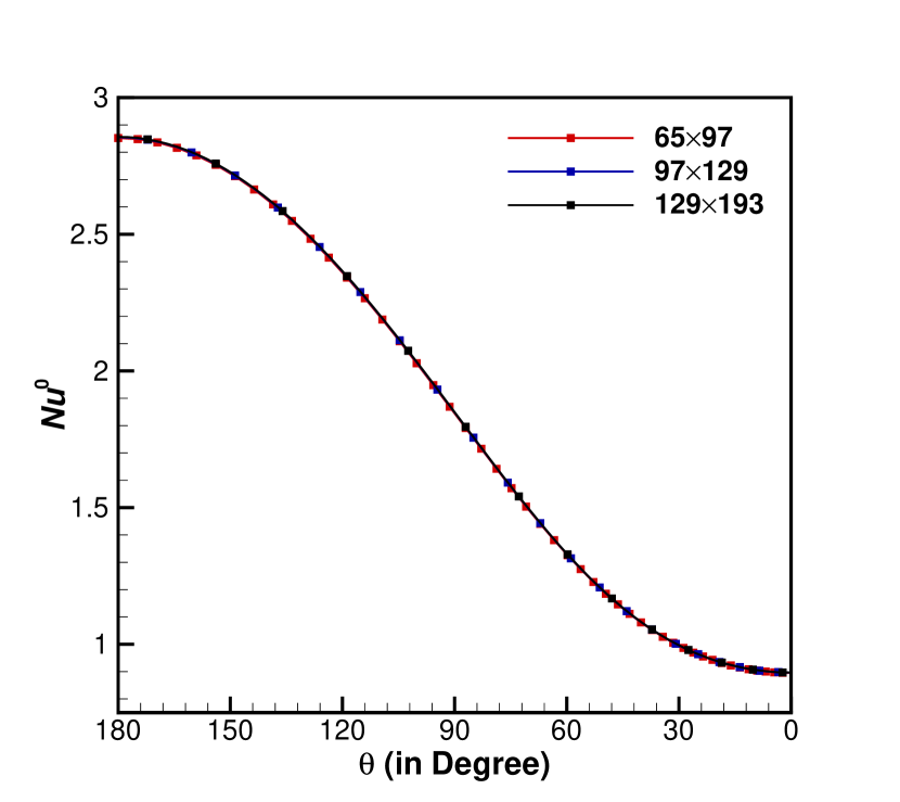
b

Figure 15: Problem 4: Distribution of (a) vortcity and (b) local Nusselt number at steady state along the surface of the cylinder for $Re$=10.

We start by verifying the grid-independence of the present numerical solution. Here, we compute for $Re$=10 and present the distribution of surface vorticity and local Nusselt number $(Nu^{0})$ and vorticity along the surface of the cylinder for three grids of different sizes viz. $65\times 97$, $97\times 129$ and $129\times 193$. Here, angle $\theta$ is measured in the counterclockwise direction starting from the rear stagnation point of the cylinder. One can see from the figures that the numerical results are unresponsive to the change in grid points and a grid of size $129\times 193$ is sufficient to capture the flow accurately.

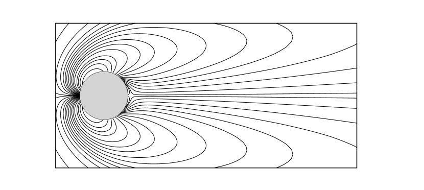
a

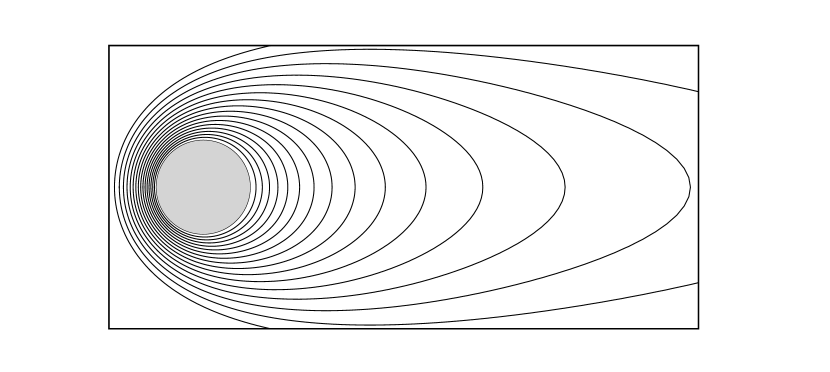
b

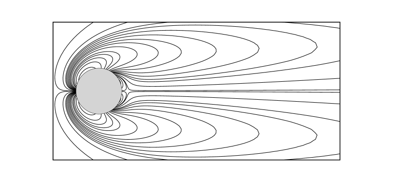
c

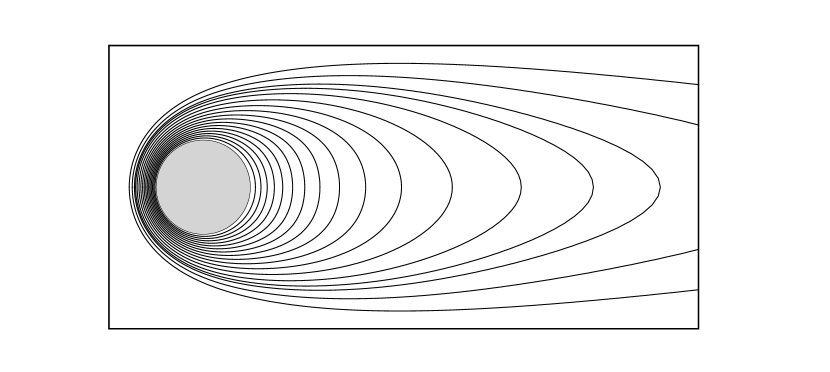
d

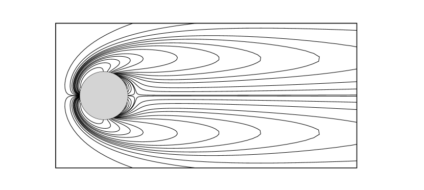
e

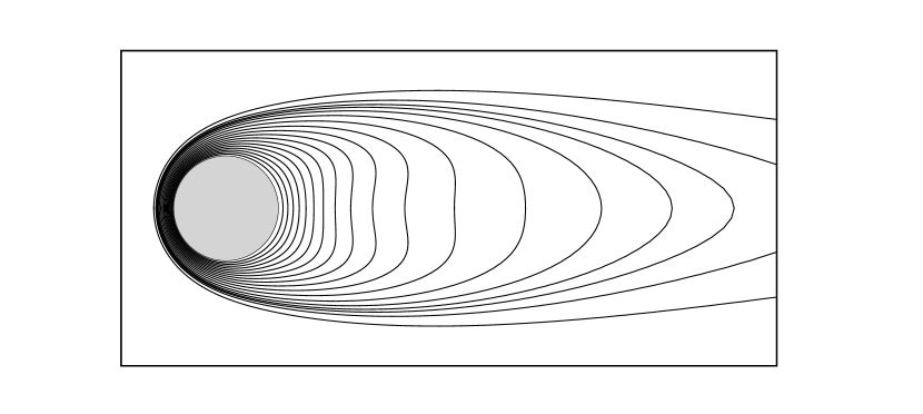
f

Figure 16: Problem 4: Steady state streamlines (left), vortifity contours (middle) and isotherms for (a) $Re$=10, (b) $Re$=20 and (c) $Re$=40.

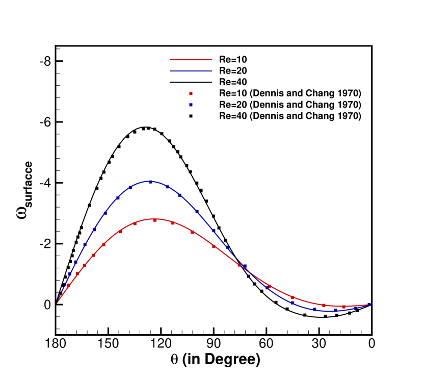
a

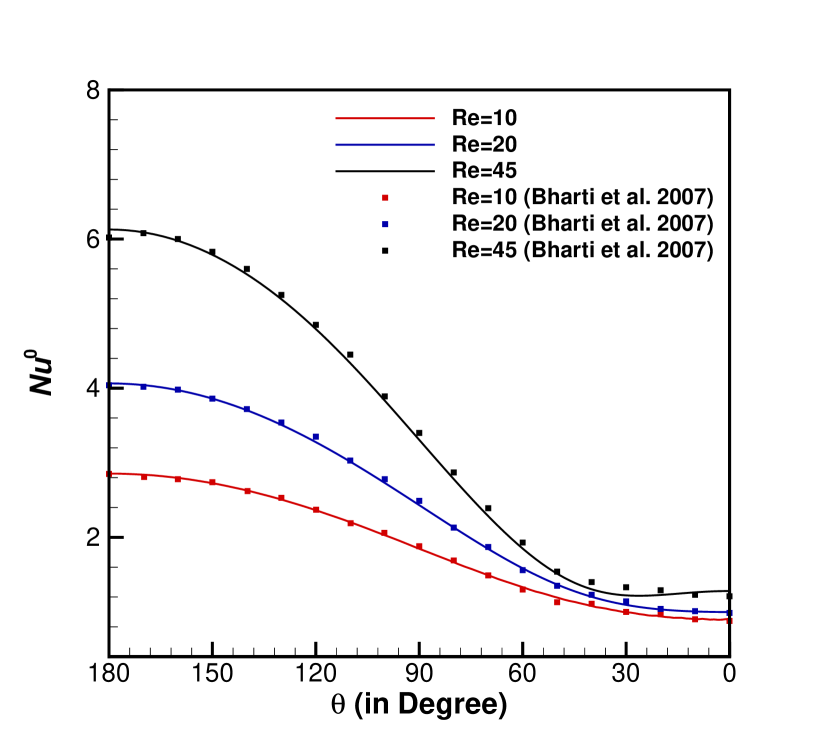
b

Figure 17: Problem 4: Comparison of (a) surface vorticity distribution for $Re$=10, 20 and 40 and (b) local Nusselt number distribution for $Re$=10, 20 and 45 with existing numerical results [44, 28].

Table 8: Problem 4: Comparison of steady state wake length, separation angle and drag coefficient for different $Re$.

		$Re$=10	$\%$-diff.		$Re$=20	$\%$-diff.		$Re$=40	$\%$-diff.
$L/D$	[31]	0.237	4.22		0.921	0.54		2.245	0.36
	[34]				0.945	3.07		2.26	0.31
	[35]				0.885	3.50		2.105	7.03
	[38]				0.93	1.51		2.31	2.47
	[8]				0.917	0.11		2.207	2.08
	[17]	0.252	1.98		0.926	1.08		2.323	3.01
	[29]				0.95	3.58		2.39	5.73
	[32]	0.266	7.14		0.937	2.24		2.139	5.33
	Present	0.247			0.916			2.253
$C_{D}$	[31]	3.170	10.50		2.152	4.23		1.499	2.33
	[34]				2.144	3.68		1.589	3.46
	[35]				2.0597	0.06		1.5308	0.21
	[38]				2.091	1.43		1.565	1.98
	[8]				2.0193	2.07		1.5145	1.29
	[17]	2.699	5.11		1.949	5.75		1.439	6.60
	[29]				2.119	2.74		1.582	3.03
	[32]	2.690	5.46		2.160	4.58		1.576	2.66
	Present	2.837			2.061			1.534
$\mkern 1.5mu\overline{\mkern-1.5muNu\mkern-1.5mu}\mkern 1.5mu$	[30]	1.8673	0.37		2.5216	2.32		3.4317	4.48
	[33]	1.8101	2.57		2.4087	2.26		3.2805	0.08
	[37]	1.6026	15.86		2.2051	11.70		3.0821	6.35
	[36]	1.8600	0.18		2.4300	1.36		3.2000	2.43
	[28]	1.8623	0.30		2.4653	0.09		3.2825	0.14
	[29]	1.8671	0.56		2.4718	0.35		3.2912	0.41
	Present	1.8567			2.4631			3.2778

A validation study is first carried out for low Reynolds number flow. At the low Reynolds number range $Re\leq 50$, the vortex structure in the wake remains steady and symmetric, thus the temperature field shows similar steady and symmetric characteristics as well. Here we select to work with $Re$=10, 20, 40, and 45. Fig. 16 depicts the symmetric vorticity and isotherm contours at steady state for various Reynolds numbers. Similar vorticity and isotherm patterns can be found in various studies available in the literature.

Present results of vorticity distribution on the cylinder surface for $Re$=10, 20 and 40 and local Nusselt number distribution for $Re$=10, 20 and 45 are portrayed in fig. 17 and 17 respectively; these values are compared with the previous numerical results from Dennis and Chang [44] and Bharti et al. [28]. It can be seen that the two sets of data show excellent agreement with each other. The largest value of the local Nusselt number is obtained at the front stagnation point of the cylinder; the value of the Nusselt number then reduces gradually towards the rear stagnation point and attains its lowest value thereat (see fig. 17). In table 8, we have compiled our computed values of $L/D$, where $L$ is the length of the recirculation bubbled formed behind the cylinder, the drag coefficient $C_{D}$ and the average Nusselt number $\mkern 1.5mu\overline{\mkern-1.5muNu\mkern-1.5mu}\mkern 1.5mu$ for $Re$=10, 20 and 40. As can be seen from the figures and table, the length of the recirculation region and the average Nusselt number depend directly on the value of the Reynolds number, while the drag coefficient varies inversely. A quantitative comparison is also carried out in table 8. Computational results are compared with reference data [28, 29, 30, 31, 8, 32, 33, 34, 35, 17, 36, 37, 38]. Once again, the efficiency of the present scheme is evident from the proximity of our results with the well-established results available in the literature.

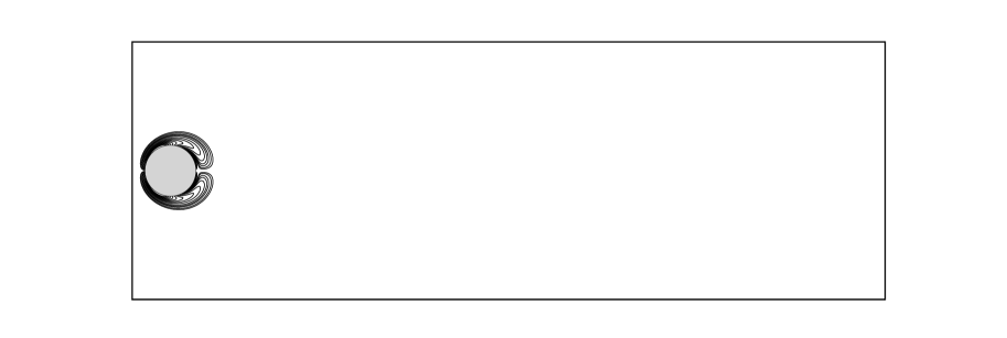
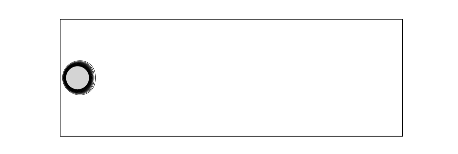
a

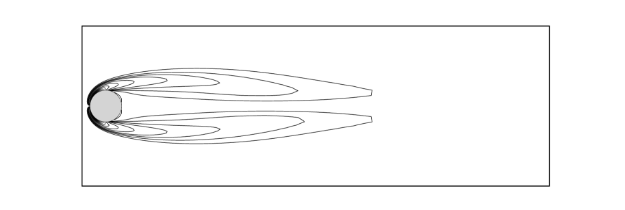
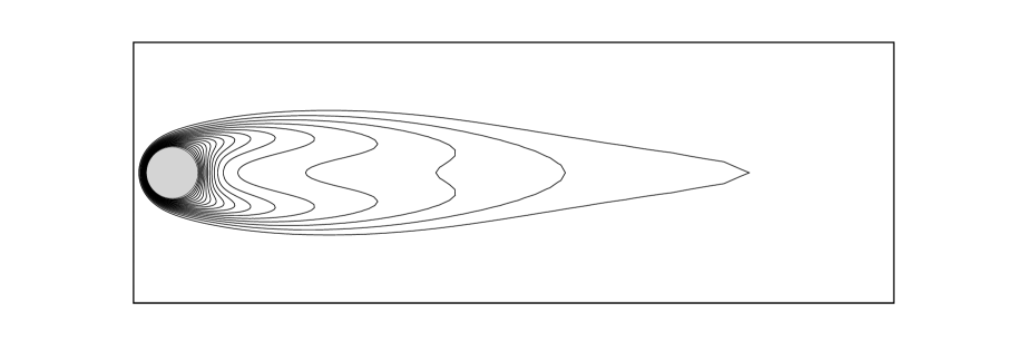
b

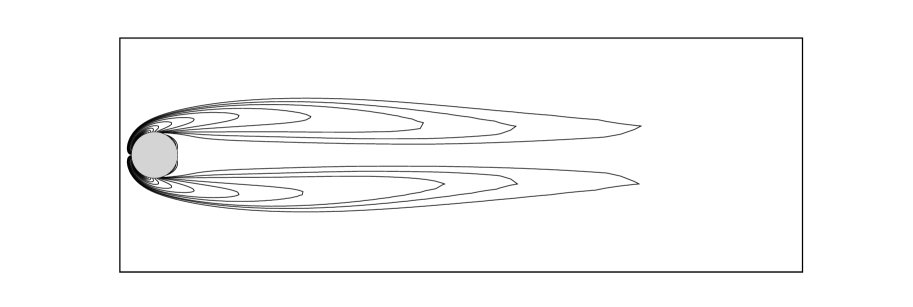
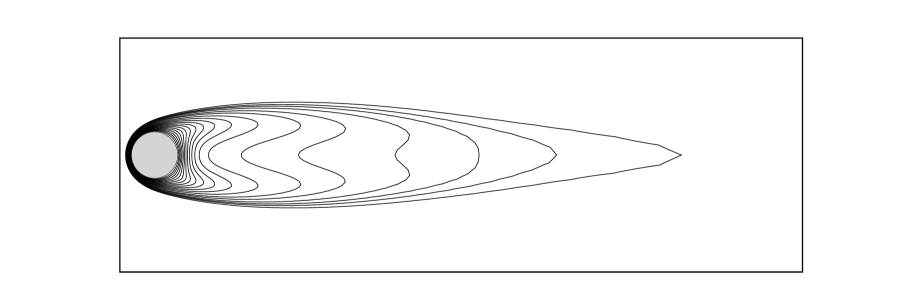
c

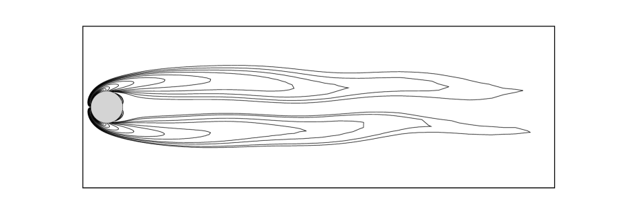
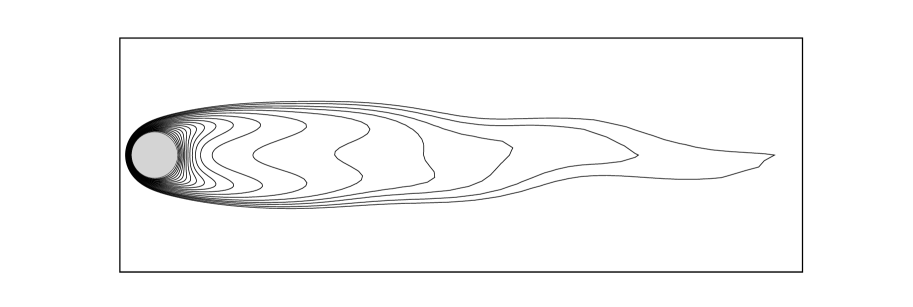
d

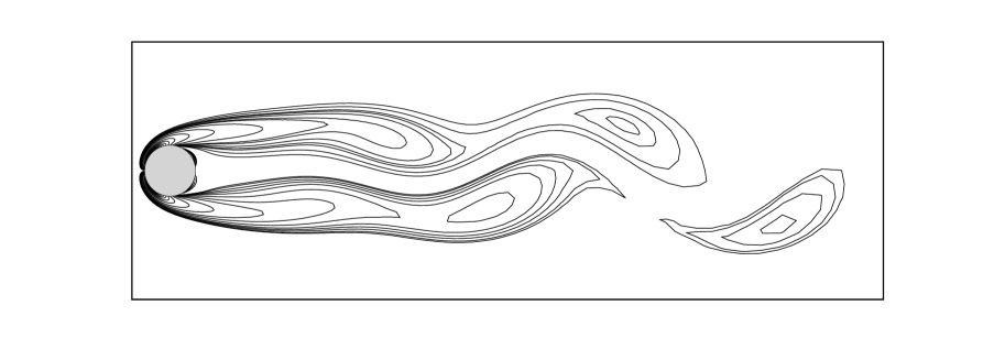
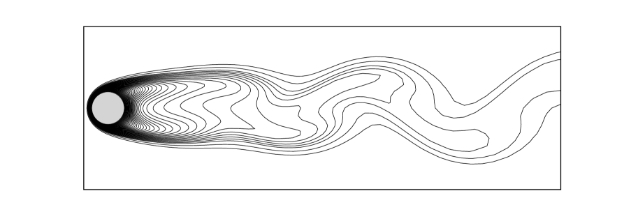
e

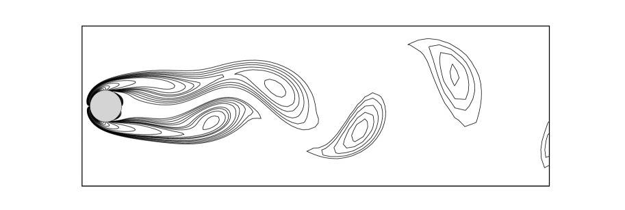
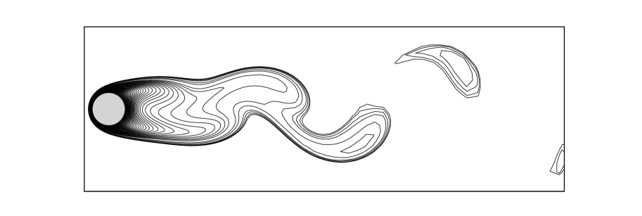
f

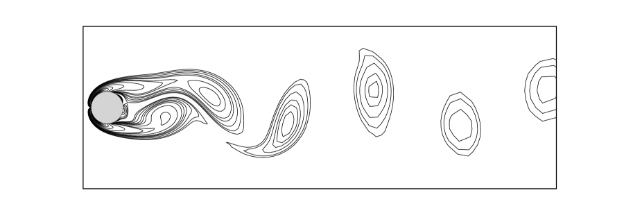
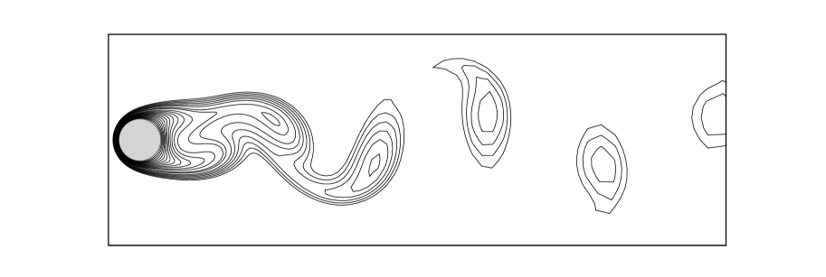
g

Figure 18: Problem 4: Evolution of vorticity (left) and isotherms (right) for $Re$=100 at (a) $t$=0.5, (b) $t$=25, (c) $t$=50, (d) $t$=75, (e) $t$=90, (f) $t$=100, (g) $t$=250.

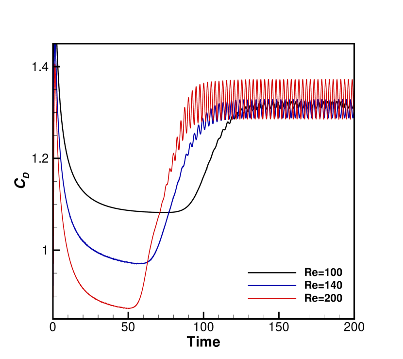
a

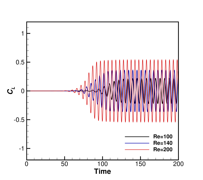
b

c

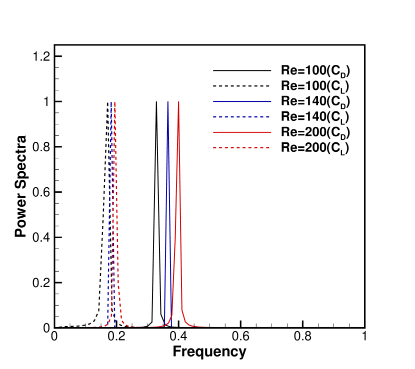
d

Figure 19: Problem 4: Temporal evolution of (a) drag coefficient, (b) lift coefficient, (c) average Nusselt number at the cylinder surface, (d) power spectra of drag and lift coefficient for $Re$=100, 140 and 200.

Next, we are interested in studying the periodic flow for $Re$=100, 140, and 200. The transition of the vorticity and isotherm contours from steady to periodic state for $Re$=100 is depicted in fig. 18. This may be considered as the representation of the flow for the other $Re$ values considered, although each requires a different time to attain periodicity. As can be seen in fig. 18, no vortex structure formed in the flow field, and the heated cylinder generates a thermal boundary layer near its surface at the beginning. As time marches, two opposite symmetrical vortices are formed simultaneously which grow in width and length with time, and remain symmetrically stable for a certain period as shown in figs. 18 and 18. During this period, the thickness of the thermal boundary layer increases; the temperature distribution also remains symmetric about the line $\theta=0$. After a certain point of time, a fluctuation develops in the flow which destroys the symmetry in the vortices and temperature distribution and they start to oscillate downstream which can be noticed in fig. 18. As the flow develops further, the vortices at the rear of the cylinder grow in size and ultimately are shed from the cylinder towards downstream while heat is carried away. It is heartening to see that the present scheme could capture the characteristic feature of the periodic flow, the so-called von Kármán vortex street very efficiently. With the vortex shedding taking place, isolated hot fluid clusters are observed in the flow (see fig. 18). Subsequently, figs. 18 and 18 indicate the synchronized variation of flow and temperature fields, where vortex shedding phenomena play a determinant role in the heat transfer at the downstream.

The time history of the drag coefficient $(C_{D})$, lift coefficient $(C_{l})$ and average Nusselt number $(\mkern 1.5mu\overline{\mkern-1.5muNu\mkern-1.5mu}\mkern 1.5mu)$ displayed in figs. 19, 19 and 19 pertinently implies that the newly developed scheme has accurately captured the periodic state for all the Reynolds numbers under consideration. The periodicity is further justified by the single dominating peak for $C_{D}$ and $C_{L}$ in the spectral density analysis (see fig. 19). The distribution of local Nusselt number $(Nu^{0})$ over the surface of the cylinder for different $Re$ values are represented in fig. 20. In fig. 20 we carry out a qualitative comparison between the surface distribution of $Nu^{0}$ for $Re$=200 computed in the present study with those of [45, 46]; which reveal close agreement of our results with those taken from the literature. We then compare our numerical values of the flow parameters $C_{d}$, $C_{l}$, $St$ and $\mkern 1.5mu\overline{\mkern-1.5muNu\mkern-1.5mu}\mkern 1.5mu$ with existing studies in table 9. The streakline from our simulation depicting the well-known von Kármán vortex street for $Re$=140 is presented in LABEL:{4fig:P5_streak140} along with the streakline reported in the experimental work of Taneda [47]. From the comparison we note that vortex creation and dissipation as captured in the experimental work is effectively computed by the current formulation. Striking similarity between our numerical results and the existing numerical and experimental results for all the cases indeed verify and validate the scheme.

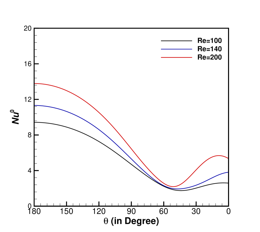
a

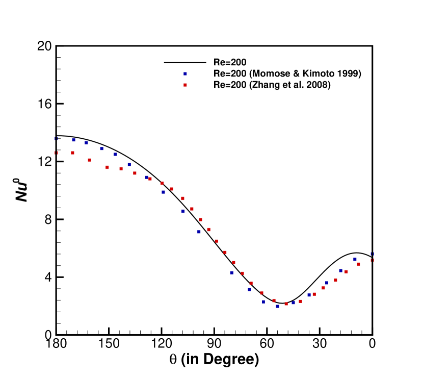
b

Figure 20: Problem 4: (a) Distribution of local Nusselt number on the cylinder surface for $Re$=100, 140, 200 and (b) comparison of local Nusselt number distribution over the cylinder surface for $Re$=200 with results from [45, 46].

Table 9: Problem 4: Comparison flow parameters $C_{D}$, $C_{L}$, $St$ and $\mkern 1.5mu\overline{\mkern-1.5muNu\mkern-1.5mu}\mkern 1.5mu$ for different $Re$.

		$Re$=100		$Re$=140		$Re$=200
$C_{D}$	[48]	1.37 $\pm$ 0.009				1.34 $\pm$ 0.030
	[49]	1.38 $\pm$ 0.010				1.37 $\pm$ 0.046
	[50]	1.394 $\pm$ 0.007				1.357 $\pm$ 0.038
	[51]	1.325 $\pm$ 0.026				1.333 $\pm$ 0.046
	Present	1.317 $\pm$ 0.008		1.308 $\pm$ 0.020		1.329 $\pm$ 0.043
$C_{L}$	[48]	$\pm$ 0.323				$\pm$ 0.430
	[49]	$\pm$ 0.340				$\pm$ 0.700
	[50]	$\pm$ 0.191				$\pm$ 0.453
	[51]	$\pm$ 0.306				$\pm$ 0.351
	Present	$\pm$ 0.22		$\pm$ 0.361		$\pm$ 0.543
$St$	[48]	0.160				0.187
	[49]	0.169				0.200
	[50]	0.165				0.197
	[51]	0.162				0.200
	Present	0.172		0.183		0.195
$\mkern 1.5mu\overline{\mkern-1.5muNu\mkern-1.5mu}\mkern 1.5mu$	[52]	5.12		5.87		7.15
	[53]	5.26				7.67
	[46]					7.23
	[54]	5.07		6.08
	Present	5.02		6.20		7.55

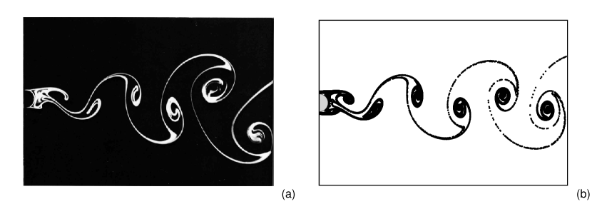
Figure 21: Problem 4: Comparison between the instantaneous streaklines for $Re$=140 captured in the (a) experimental study of Taneda [47] and (b) present computation.

5 Conclusion

In this work, we extend the philosophy of recent work on 2D transient convection and diffusion equation on Cartesian coordinates [18] to polar coordinates to tackle non-rectangular geometries. The transformation-free higher-order compact finite difference scheme proposed here can be applied directly on polar grids, unlike most of the schemes in the literature on polar grids that use transformation between physical and computational domains. We have also combined the virtue of nonuniformity with the present scheme. This levitates the efficiency and robustness of the scheme as it acquires the advantage of accumulating and scattering grid points as necessary. The scheme is theoretically third-order accurate in space and second-order accurate temporally. It is worthwhile to mention that for linear problem with analytical solution the scheme exhibits a spatial convergence of order four, which is higher than the theoretical value. The robustness of the scheme is examined by applying it to as many as three benchmark problems of fluid flow and heat flow, viz. driven polar cavity, natural convection in a horizontal concentric annulus, and forced convection around a heated stationary cylinder. In order to resolve the Neumann type boundary conditions, we have also introduced one-sided approximations for first order derivatives. For the problem of forced convection around a heated stationary cylinder, both steady and periodic solutions are being accurately captured by the present scheme. Additionally, important aspects such as the von Kármán vortex phenomenon and the effect of vortex shedding on heat transfer are also studied comprehensively for this fluid body interaction problem. The accuracy of the computed solutions is estimated from the results obtained in all the test problems, which are in excellent agreement with the existing results both qualitatively and quantitatively. We have reported the perceived order of convergence for all the variables in flow problems that are not supplemented with analytical solutions. It is heartening to see that our solutions could attain the theoretical order of convergence in both space and time in all cases.

References

- Iyengar and Manohar [1988] S. R. K. Iyengar and R. Manohar. High order difference methods for Heat equation in polar cylindrical coordinates. Jouirnal of Computational Physics, 77:425–438, 1988.
- Jain et al. [1994] M. K. Jain, R. K. Jain, and M. Krishna. A fourth-order difference scheme for quasilinear Poisson equation in Polar co-ordinates. Communications in Numerical Methods in Engineering, 10:791–797, 1994.
- Borges and Daripa [2001] L. Borges and P. Daripa. A fast parallel algorithm for the Poisson equation on a disk. Jouirnal of Computational Physics, 169:151–192, 2001.
- Lai and Wang [2001] M. C. Lai and W. C. Wang. Fast direct solvers for Poisson equation on 2D polar and spherical geometries. Numerical Methods for Partial Differential Equations, 18(1):56–68, 2001.
- Zhuang and Sun [2001] Y. Zhuang and X. H. Sun. A high-order fast direct solver for singular Poisson equations. Journal of Computational Physics, 171:79–94, 2001.
- Lai [2002] M. C. Lai. A simple compact fourth-order Poisson solver on polar geometry. Journal of Computational Physics, 182:337–345, 2002.
- Sanyasiraju and Manjula [2005] Y. V. S. S. Sanyasiraju and V. Manjula. Flow past an impulsively started circular cylinder using a higher-order semicompact scheme. Physical Review E, 72:016709, 2005.
- Kalita and Ray [2009] J. C. Kalita and R. K. Ray. A transformation-free HOC scheme for incompressible viscous flows past an impulsively started circular cylinder. Journal of Computational Physics, 228:5207–5236, 2009.
- Ray and Kalita [2010] R. K. Ray and J. C. Kalita. A transformation-free HOC scheme for incompressible viscous flows on nonuniform polar grids. International Journal for Numerical Methods in Fluids, 62:683–708, 2010.
- Yu and Tian [2013] P. X. Yu and Z. F. Tian. A compact scheme for the streamfunction-velocity formulation of the 2d steady incompressible navier-stokes equations in polar coordinaes. Journal of Scientific Computing, 56:165–189, 2013.
- Das et al. [2023] P. Das, S. K. Pandit, and R. K. Ray. A new perspective of higher order compact nonuniform padé approximation based finite difference scheme for solving incompressible flows directly on polar grids. Computers and Fluids, 254:105793, 2023.
- Lele [1992] S. K. Lele. Compact finite difference schemes with spectral-like resolution. Journal of Computational Physics, 103:16–42, 1992.
- Sen et al. [2013] S. Sen, J. C. Kalita, and M. M. Gupta. A robust implicit compact scheme for two-dimensional unsteady flows with a biharmonic stream function formulation. Computers and Fluids, 84:141–163, 2013.
- Sen [2013] S. Sen. A new family of (5,5)CC-4OC schemes applicable for unsteady Navier-Stokes equations. Journal of Computational Physics, 251:251–271, 2013.
- Fuchs and Tillmark [1985] L. Fuchs and N. Tillmark. Numerical and experimental stiudy of driven flow in a polar cavity. International Journal for Numerical Methods in FLuids, 5:311–329, 1985.
- Lee and Tsuei [1993] D. Lee and Y. M. Tsuei. A hybrid adaptive gridding procedure for recirculating fluid flow problem. Journal of Computational Physics, 108:122–141, 1993.
- Sen and Kalita [2015] S. Sen and J. C. Kalita. A 4OEC scheme for the biharmonic steady Navier-Stokes equation in non-rectangular domains. Computer Physics Communications, 196:113–133, 2015.
- Deka and Sen [2021] D. Deka and S. Sen. A new transformation free generalized (5,5)HOC discretization of transient Navier-Stokes/Boussinesq equations on nonuniform grids. International Journal of Heat and Mass Transfer, 171:120821, 2021.
- Crawford and Lemlich [1962] L. Crawford and R. Lemlich. Natural convection in horizontal concentric cylindrical annuli. Industrial & Engineering Chemistry fundamentals, 1:260–264, 1962.
- Powe et al. [1971] R. E. Powe, C. T. Carley, and S. L. Carruth. A numerical solution for natural convection in cylindrical annuli. Journal of Heat Transfer, 92(12):210–220, 1971.
- Kuehn and Goldstein [1976] T. H. Kuehn and R. J. Goldstein. An experimental and theoretical study of natural convection in the annulus between horizontal concentric cylinders. Journal of Fluid Mechanics, 74(4):695–719, 1976.
- Mack and Bishop [1968] L. R. Mack and E. H. Bishop. Natural convection between horizontal concentric cylinders for low Rayleigh numbers. Quarterly Journal of Mechanics and Applied Mathematics, 21:223–241, 1968.
- Tsui and Tremblay [1984] Y. T. Tsui and B. Tremblay. On transient natural convection heat transfer in the annulus between concentric, horizontal cylinders with isothermal surfaces. Internatioanl Journal Heat and Mass Transfer, 27(1):103–111, 1984.
- Shahraki [2002] F. Shahraki. Modeling of buoyancy-driven flow and heat transfer for air in a horizontal annulus: effects of vertical eccentricity and temperature-dependent properties. Numerical Heat Transfer, Part A, 42:603–621, 2002.
- Shi et al. [2006] Y. Shi, T. S. Zhao, and Z. L. Guo. Finite difference-based lattice Boltzmann simulation of natural convection heat transfer in a horizontal concentric annulus. Computers and Fluids, 35:1–15, 2006.
- Yang and Kong [2019] X. Yang and S. C. Kong. Numerical study of natural convection in a horizontal concentric annulus using smoothed particle hydrodynamics. Engineering Analysis with Boundary Elements, 102:11–20, 2019.
- Zhang and Yang [2023] W. Zhang and X. Yang. SPH modeling of natural convection in horizontal anuuli. Acta Mechanica Sinica, 39:322093, 2023.
- Bharti et al. [2007] R. P. Bharti, R. Chhabra, and V. Eswaran. A numerical study of the steady forced convection heat transfer from an unconfined circular cylinder. Heat and Mass Transfer, 43:639–648, 2007.
- Chen et al. [2020] Z. Chen, C. Shu, L. M. Yang, X. Zhao, and N. Y. Liu. Immersed boundary–simplified thermal lattice Boltzmann method for incompressible thermal flows. Physics of Fluids, 32:013605, 2020.
- Dennis et al. [1968] S. C. R. Dennis, J. D. Hudson, and N. Smith. Steady laminar forced convection from a circular cylinder at low Reynolds numbers. Physics of Fluids, 11:933–940, 1968.
- He and Doolen [1997] X. He and G. Doolen. Lattice Boltzmann method on curvilinear coordinate system: flow around a circular cylinder. Journal of Computational Physics, 134:306–315, 1997.
- Kumar and Kalita [2021] P. Kumar and J. C. Kalita. A comprehensive study of secondary and tertiary vortex phenomena of flow past a circular cylinder: A cartesian grid approach. Physics of Fluids, 33:053608, 2021.
- Lange et al. [1998] C. Lange, F. Durst, and M. Breuer. Momentum and heat transfer from cylinders in laminar crossflow at . International Journal of Heat and Mass Transfer, 41:3409–3430, 1998.
- Niu et al. [2006] X. Niu, C. Shu, Y. Chew, and Y. Peng. A momentum exchange-based immersed boundary-lattice boltzmann method for simulating incompressible viscous flows. Physics Letters A, 354:173–182, 2006.
- Sanyasiraju and Mishra [2008] Y. V. S. S. Sanyasiraju and N. Mishra. Spectral resolutioned exponential compact higher order scheme (SRECHOS) for convection-diffusion equations. Computer Methods in Applied Mechanics and Engineering, 197:4737–4744, 2008.
- Soares et al. [2005] A. Soares, J. Ferreira, and R. Chhabra. Flow and forced convection heat transfer in crossflow of non-Newtonian fluids over a circular cylinder. Industrial & Engineering Chemistry Research, 44:5815–5827, 2005.
- Sparrow et al. [2004] E. M. Sparrow, J. P. Abraham, and J. C. Tong. Archival correlations for average heat transfer coefficients for non-circular and circular cylinders and for spheres in cross-flow. International Journal of Heat and Mass Transfer, 47:5285–5296, 2004.
- Wu and Shu [2009] J. Wu and C. Shu. Implicit velocity correction-based immersed boundary lattice Boltzmann method and its applications. Journal of Computational Physics, 228:1963–1979, 2009.
- Franke et al. [1990] R. Franke, W. Rodi, and B. Schönung. Numerical calculation of laminar vortex-shedding flow past cylinder. Journal of Wind Engineering and Industrial Aerodynamics, 35:237–257, 1990.
- Breuer [1998] M. Breuer. Large eddy simulation of the subcritical flow past a circular cylinder: numerical and modeling aspects. International Journal for Numerical Methods in Fluids, 28:1281–1302, 1998.
- Kalita and Sen [2012] J. C. Kalita and S. Sen. The biharmonic approach for unsteady floe past an impulsively started cilrcular cylinder. Computers and Fluids, 59:44–60, 2012.
- Lankadasu and Vengadesan [2010] A. Lankadasu and S. Vengadesan. Shear effect on square cylinder wake transition characteristics. International Journal for Numerical Methods in Fluids, 67:1112–1134, 2010.
- Wang et al. [2009] Z. Wang, J. Fan, and K. Cen. Immersed boundary method for the simulation of 2d viscous flow based on vorticity-velocity formulations. Journal of Computational Physics, 228:1504–1520, 2009.
- Dennis and Chang [1970] S. C. R. Dennis and G. Z. Chang. Numerical solution for steady flow past a circular cylinder at Reynolds numbers up to 100. Journal of Fluid Mechanics, 42(3):471–489, 1970.
- Momose and Kimoto [1999] K. Momose and H. Kimoto. Forced convection heat transfer from a heated circular cylinder with arbitrary surface temperature distributions. Heat Transfer—Asian Research, 28(6):484–499, 1999.
- Zhang et al. [2008] N. Zhang, Z. C. Zheng, and S. Eckels. Study of heat-transfer on the surface of a circular cylinder in flow using an immersed-boundary method. International Journal of Heat and Fluid Flow, 29:1558–1566, 2008.
- Taneda [1979] S. Taneda. Visualization of separating stokes flows. Journal of the Physical Society of Japan, 46(6):1935–1942, 1979.
- Le et al. [2006] D. V. Le, B. C. Khoo, and J. Peraire. An immersed interface method for viscous incompressible flows involving rigid and flexible boundaries. Journal of Computational Physics, 220:109–138, 2006.
- Berthelsen and Faltinsen [2008] P. A. Berthelsen and O. M. Faltinsen. A local directional ghost cell approach for incompressible viscous flow problems with irregular boundaries. Journal of Computational Physics, 227:4354–4397, 2008.
- Sen [2012] S. Sen. Compact biharmonic computation of the Navier-Stokes equations: Extension to complex flows. PhD thesis, 2012.
- Kumar and Kalita [2019] P. Kumar and J. C. Kalita. A transformation-free formulation of the Navier–Stokes equations on compact nonuniform grids. Journal of Computational and Applied Mathematics, 353:292–317, 2019.
- Churchill and Bernstein [1977] S. W. Churchill and M. Bernstein. A correlating equation for forced convection from gases and liquids to a circular cylinder in crossflow. ASME. Journal of Heat Transfer, 99(2):300–306, 1977.
- Cheng and Hong [1997] C. H. Cheng and J. L. Hong. Numerical prediction of lock-on effect on convective heat transfer from a transversely oscillating circular cylinder. International Journal of Heat and Fluid Flow, 40(8):1825–1834, 1997.
- Cao et al. [2021] S. L. Cao, X. Sun, J. Z. Zhang, and Y. X. Zhang. Forced convection heat transfer around a circular cylinder in laminar flow: An insight from Lagrangian coherent structures. Physics of Fluids, 33:067104, 2021.