Generalized Symmetry in Dynamical Gravity

Abstract

We explore generalized symmetry in the context of nonlinear dynamical gravity. Our basic strategy is to transcribe known results from Yang-Mills theory directly to gravity via the tetrad formalism, which recasts general relativity as a gauge theory of the local Lorentz group. By analogy, we deduce that gravity exhibits a one-form symmetry implemented by an operator $U_{\alpha}$ labeled by a center element $\alpha$ of the Lorentz group and associated with a certain area measured in Planck units. The corresponding charged line operator $W_{\rho}$ is the holonomy in a spin representation $\rho$, which is the gravitational analog of a Wilson loop. The topological linking of $U_{\alpha}$ and $W_{\rho}$ has an elegant physical interpretation from classical gravitation: the former materializes an exotic chiral cosmic string defect whose quantized conical deficit angle is measured by the latter. We verify this claim explicitly in an AdS-Schwarzschild black hole background. Notably, our conclusions imply that the standard model exhibits a new symmetry of nature at scales below the lightest neutrino mass. More generally, the absence of global symmetries in quantum gravity suggests that the gravitational one-form symmetry is either gauged or explicitly broken. The latter mandates the existence of fermions. Finally, we comment on generalizations to magnetic higher-form or higher-group gravitational symmetries.

CALT-TH 2024-009

1 Introduction

Symmetry has long been a vital tool for investigating complex physical systems, particularly at strong coupling. Historically, most efforts in this expansive subject have focused on conventional symmetries, which act on local operators. The standard model of physics exhibits numerous exact and approximate symmetries of this type, for example relating to charge in electromagnetism and chiral symmetry in the strong interactions.

In the past decade, however, the fundamental concept of symmetry has broadened considerably Alford:1991vr ; Alford:1990fc ; Alford:1992yx ; Bucher:1991bc ; Pantev:2005rh ; Pantev:2005wj ; Pantev:2005zs ; Hellerman:2006zs ; Nussinov:2009zz ; Aharony:2013hda . As described in the seminal work of Gaiotto:2014kfa , it is now understood that the traditional formulation of symmetry is actually the tip of a colossal iceberg. Rather, there exists a rich patchwork of so-called higher-form symmetries whose distinguishing feature is that they act intrinsically on extended objects described by nonlocal operators supported on lines, surfaces, and membranes. Since higher-form symmetries act trivially on local operators, their physical implications are sometimes quite subtle to diagnose. From this point of view, the standard symmetries found in most quantum field theory textbooks are brusquely relegated to the special case of zero-form symmetry.

The growing body of work on generalized symmetries has revealed new perspectives on a broad spectrum of assorted phenomena in quantum field theory, including phase transitions Iqbal:2021rkn ; Wen:2018zux ; Levin:2004mi ; Levin:2004js ; Hastings:2005xm ; Shimizu:2017asf , anomalies Choi:2022jqy ; Cordova:2022ieu ; Gaiotto:2017yup ; Wan:2018zql ; Delacretaz:2019brr ; Hsin:2018vcg ; Tanizaki:2017mtm ; Cordova:2019bsd ; Wan:2018djl ; Cordova:2019jnf ; Cordova:2019uob ; Delmastro:2022pfo , and symmetry breaking Kovner:1992pu ; Hofman:2018lfz ; Lake:2018dqm ; Sogabe:2019gif ; GarciaEtxebarria:2022jky . Recent work has even explored new opportunities for physics beyond the standard model, for example in the context of flavor physics Cordova:2022qtz , neutrinos Cordova:2022fhg , and axions Hidaka:2020iaz ; Hidaka:2020izy ; Brennan:2020ehu ; Choi:2022fgx ; Yokokura:2022alv ; Brennan:2023kpw ; Choi:2023pdp ; Cordova:2023her ; Reece:2023iqn ; Agrawal:2023sbp . Such efforts are a welcome development, as they attempt to draw an explicit connection between highly formal developments in mathematical physics and high-energy physics of actual experimental relevance. That said, the constraints imposed by generalized symmetry on particle physics models tend to be explicable via more conventional means. This is perhaps not so surprising—these models are easily embedded within renormalizable theories in which all is calculable and there are no surprises to be had or which require explanation.

Gravity, on the other hand, is another story. Far less is understood about its putative ultraviolet completion. Consequently, the only truly theory-agnostic approach is to retreat to safely low energies, where gravitational dynamics are described universally by an effective field theory of gravitons on a fixed background, augmented by possible higher-derivative corrections. For example, see Donoghue:2022eay ; Burgess:2003jk for a review of this perspective. The effective field theory of gravity is clearly a natural target for understanding generalized symmetry in a refreshingly different context. There has, however, been relatively little effort in this vein. Some notable exceptions include interesting recent work studying the higher-form symmetries associated with parity McNamara:2022lrw and topology change McNamara:2019rup , as well as generalizations of continuous higher-form symmetries to linearized gravity Hinterbichler:2022agn ; Benedetti:2021lxj ; Benedetti:2023ipt .

In this paper, we extend the now well-established insights of higher-form symmetry in gauge theory to the effective theory of nonlinear gravity in four-dimensional spacetime. Our key ingredient is the well-known fact that gravity can itself be recast in gauge theoretic language. As history would have it, this perspective carries dual meanings. On the one hand, gravity is a theory of diffeomorphisms, nonlinearly realized by a self-interacting, massless spin two field. Since diffeomorphisms are a redundancy, they are on occasion referred to as a gauge symmetry, though colloquially and not in the strict technical sense. On the other hand, it is well-known that gravity can also be described by a bona fide gauge theory of local Lorentz transformations, which is the so-called Palatini formalism for the tetrad and spin connection. Formally, these descriptions are equivalent since gauge symmetry is, after all, pure redundancy and no redundancy is more valid than any other. As we will see, tetradic Palatini gravity is perfectly suited to our purposes because we can work in lockstep analogy with the familiar approach taken in gauge theory. For concreteness, the bulk of our analysis will be in Euclidean signature, though we will toggle to Lorentzian signature on and off when needed. Our conclusions for gravity are as follows.

First and foremost, our central claim is that tetradic Palatini gravity exhibits an electric one-form symmetry described by the center subgroup $Z(G)$ of the Lorentz group $G$. This one-form symmetry depends crucially on the signature and global structure of $G$. For example, in Euclidean signature the center is nontrivial when we consider $Z({\rm SO}(4))=\mathbb{Z}_{2}$ or $Z({\rm Spin}(4))=\mathbb{Z}_{2}{\hskip 1.00006pt\times\hskip 1.00006pt}\mathbb{Z}_{2}$, while in Lorentzian signature the center is nontrivial for $Z({\rm SL}(2,\mathbb{C}))=\mathbb{Z}_{2}$. In all cases, these center subgroups have a zero-form symmetry action as various parities on Lorentz vector and spinor indices.

Second, we show how the one-form symmetry of gravity is implemented by a topological symmetry operator $U_{\alpha}$. This object is constructed explicitly in terms of the local degrees of freedom as the exponential of a certain area operator for a closed surface measured in Planck units and labeled by an element of the center ${\alpha}$. The symmetry operator $U_{\alpha}$ acts on a line operator $W_{\rho}$ known as the spin holonomy, which is simply a Wilson loop for the spin connection computed in a spin representation ${\rho}$ along a chosen contour. While $U_{\alpha}$ generates a global one-form symmetry, it can be implemented as a field transformation that is precisely the form of a local Lorentz transformation, but with nontrivial winding that precludes it from being a genuine local Lorentz transformation. Using this “twisted local Lorentz transformation”, we show that $W_{\rho}$ transforms by a center-valued phase that depends only on the topological linking of the surface and curve which define $U_{\alpha}$ and $W_{\rho}$, respectively. We prove the Ward identity for $U_{\alpha}$ and $W_{\rho}$ using both covariant and canonical approaches. Notably, this proof is valid to all orders in perturbation theory, at least within the context of the effective field theory description of gravity where the topology and dimension of spacetime are preserved.

Thirdly, we show that the interplay of $U_{\alpha}$ and $W_{\rho}$ has a remarkably simple interpretation in terms of classical gravitation. The symmetry operator $U_{\alpha}$ creates a defect in spacetime that is a chiral version of a cosmic string defect, and serves as a certain gravitational analog of the Dirac string. The tension of $U_{\alpha}$ is quantized so as to induce a $\pi$ deficit angle which is directly measured by the spin holonomy $W_{\rho}$ as the center-valued linking number. We then compute the linking number by evaluating $W_{\rho}$ on various spacetimes, including an AdS-Schwarzschild background. The topological nature of $U_{\alpha}$ implies that its linking with $W_{\rho}$ arises purely from contributions at leading order in the so-called self-force expansion, where $U_{\alpha}$ is treated as a nondynamical background. Furthermore, this implies that higher order self-force corrections are vanishing, so evidently the classical deficit angle is not quantum corrected at any perturbative order.

Last but not least, we discuss the breaking of the gravitational one-form symmetry. As expected, explicit breaking requires a local operator in the representation ${\rho}$ that renders the spin holonomy $W_{\rho}$ “endable,” thus unspooling its linking with $U_{\alpha}$. Physically, this corresponds to the screening of the spin holonomy by spinning particles. Interestingly, the spin holonomy in the vector representation is automatically screened in pure gravity by orbital angular momentum. This mirrors the phenomenon in gauge theory where adjoint Wilson lines are screened by the gluon field itself. On the other hand, holonomies in the spinor representation are endable only by local fermionic operators. If no such operators exist, then the one-form gravitational symmetry is exact. Remarkably, this implies the emergence of a hidden symmetry of the real world: below the lightest neutrino mass, there is a gravitational one-form symmetry under which spinor holonomies are charged. More generally, in a theory in which the gravitational one-form symmetry is not gauged, the conjectured absence of exact global symmetries in quantum gravity directly implies the existence of fermions.

2 Gauge Theory

In this section, we present a self-contained review of one-form symmetries in gauge theory. Other treatments can be found in the literature Gomes:2023ahz ; Brennan:2023mmt ; Schafer-Nameki:2023jdn ; McGreevy:2022oyu ; Cordova:2022ruw ; witten230b ; Bhardwaj:2023kri . We start with a covariant analysis expressed in the language of path integrals, followed by a treatment in terms of canonical quantization. Because this section is mostly—though not entirely—a recap of known results from gauge theory, it may be skipped by readers interested only in our new findings, which pertain to gravity. However, we note that this gauge theory warm up forms a concrete road map for our parallel analysis of gravity later on.

2.1 Covariant Formalism

To begin, let us consider Yang-Mills theory for a gauge group $G$ which is a connected matrix Lie group. We take spacetime to be a Riemannian four-manifold ${\mathcal{M}}$ of Euclidean signature. Our discussion will apply irrespective of whether or not the background spacetime is curved, provided it is nondynamical. As is well-known, this theory admits a first-order formulation in terms of a one-form gauge connection and an auxiliary two-form field,

$$A^{a}=A^{a}{}_{\mu}\hskip 1.00006ptdx^{\mu}\qquad\resizebox{}{}{\scalebox{0.95}[0.95]{{\leavevmode\hbox{\set@color{\text{and}}}}}}\qquad B_{a}=\frac{1}{2}\hskip 1.00006ptB_{a\mu\nu}\hskip 1.00006ptdx^{\mu}{\hskip 1.00006pt{\wedge}\,}dx^{\nu}\,,$$ (1)

valued in the adjoint and the coadjoint of $G$, respectively, so $a,b,\ldots\in\{1,\ldots,{\rm dim}(G)\}$. The action is the integral over ${\mathcal{M}}$ of the Lagrangian four-form,

$$L=\frac{1}{g^{2}}\hskip 1.00006ptB_{a}{\hskip 1.00006pt{\wedge}\,}F^{a}-\frac{1}{2g^{2}}B_{a}{\hskip 1.00006pt{\wedge}\,}{*}B^{a}\qquad\resizebox{}{}{\scalebox{0.95}[0.95]{{\leavevmode\hbox{\set@color{\text{where}}}}}}\qquad F^{a}=dA^{a}+\frac{1}{2}\hskip 1.00006ptf^{a}{}_{bc}\hskip 1.00006ptA^{b}\wedge A^{c}\,,$$ (2)

where $g$ is the gauge coupling. Throughout, color indices are raised and lowered by the Killing form, while the Hodge dual $*$ with respect to the background metric acts on spacetime indices. Integrating out the auxiliary two-form field enforces $B_{a}=*F_{a}$, and plugging this back in to Eq. (2), we obtain $(1/2g^{2})\hskip 1.00006ptF_{a}{\hskip 1.00006pt{\wedge}\,}{*}F^{a}$, which is the textbook Lagrangian for Yang-Mills theory in a fixed background spacetime.

2.1.1 Line and Symmetry Operators

In Yang-Mills theory, the one-form symmetry group is identified with the center of the gauge group, $Z(G)$. By definition, the one-form symmetry acts on extended objects rather than local operators. The relevant charged object is the one-dimensional line operator,

$$W_{\rho}({\mathcal{C}})=\operatorname{tr}_{{\rho}}\mathrm{P}\kern-1.00006pt\exp\bigg{(}\hskip 0.50003pt{\oint_{{\mathcal{C}}}A}\bigg{)}\,,$$ (3)

which is a path-ordered Wilson loop along a closed contour ${\mathcal{C}}$. Here ${\rho}$ denotes the irreducible representation in which the trace and exponentiation are defined.

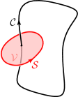
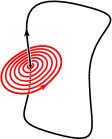
Figure 1: Left: The linking number between a one-dimensional contour ${\mathcal{C}}$ and an exact codimension two surface ${\mathcal{S}}=\partial{\mathcal{V}}$ is equal to the number of intersections between the coboundary ${\mathcal{V}}$ and ${\mathcal{C}}$. Right: The coboundary ${\mathcal{V}}$ defines a homotopy for shrinking the surface ${\mathcal{S}}$ to a point on ${\mathcal{C}}$.

Meanwhile, the one-form symmetry transformation is implemented by a corresponding symmetry operator,

$$U_{\alpha}({\mathcal{S}})\,,$$ (4)

which is an instance of the Gukov-Witten operator Gukov:2006jk . This operator is supported on a two-dimensional surface ${\mathcal{S}}$ and labeled by a center element $\alpha{\,\in\,}Z(G)$. We will present a concrete formula for $U_{\alpha}({\mathcal{S}})$ in terms of explicit fields later on. But for the moment, let us abstractly describe the symmetry operator in terms of the defining property that it generates the following transformation on the line operator,

$$W_{\rho}({\mathcal{C}})\,\,\mapsto\,\,{\rho}({\alpha})^{\operatorname{link}({\mathcal{C}},{\mathcal{S}})}\hskip 1.00006ptW_{\rho}({\mathcal{C}})\,,$$ (5)

where ${\rho}({\alpha})$ is the representation of the center element ${\alpha}$ as a complex phase, and we have defined $\operatorname{link}({\mathcal{C}},{\mathcal{S}})$ to be the linking number between the contour ${\mathcal{C}}$ and the surface ${\mathcal{S}}$. Crucially, since the linking number is a topological invariant, so too is the operator $U_{\alpha}({\mathcal{S}})$, in the sense that the surface of its support ${\mathcal{S}}$ can be deformed arbitrarily to yield the same action on the Wilson loop $W_{\rho}({\mathcal{C}})$ provided it does not degenerate with ${\mathcal{C}}$.

In this paper, we will always assume that the two-dimensional support of the symmetry operator is not only closed but also exact, so the surface ${\mathcal{S}}=\partial{\mathcal{V}}$ is the boundary of a three-dimensional volume ${\mathcal{V}}$. This is required so that the symmetry operator can be contracted continuously into an infinitesimal two-sphere enclosing the line operator, as depicted in Fig. 1. Intuitively, this deformation corresponds to the physical measurement of the electric charge of a body by computing the electric flux flowing through an infinitesimal two-sphere enclosing it. As a consequence, we see that

$$\operatorname{link}({\mathcal{C}},{\mathcal{S}})=\operatorname{int}({\mathcal{C}},{\mathcal{V}})\qquad\resizebox{}{}{\scalebox{0.95}[0.95]{{\leavevmode\hbox{\set@color{\text{where}}}}}}\qquad{\mathcal{S}}=\partial{\mathcal{V}}\,.$$ (6)

so the linking number between ${\mathcal{S}}$ and ${\mathcal{C}}$ is equal to the intersection number between ${\mathcal{C}}$ and the coboundary ${\mathcal{V}}$.

In Maxwell theory, it is well-known that the one-form symmetry is implemented by a shift of the gauge field by a “flat connection”, which is closed wherever it is well-defined and nonsingular, but crucially not exact. A key fact that we now emphasize is that this can be realized as a transformation of the fields that takes the form of a gauge transformation for a multivalued—that is, winding—gauge parameter, which is hence is not globally defined. For instance, consider the map $A\mapsto A+d\chi$. If the zero-form parameter $\chi$ exhibits nontrivial winding, then $d\chi$ is not, despite its appearance, an exact form. For example, we might choose $\chi=\varepsilon\hskip 1.00006pt\phi$, where $\varepsilon$ is a constant and $\phi$ is the azimuthal angle in cylindrical coordinates. Crucially, $d\phi=(x\hskip 1.00006ptdy{\,-\,}y\hskip 1.00006ptdx)/(x^{2}{\,+\,}y^{2})$ is not exact because its integral around a closed circular loop, $\int_{S^{1}}d\phi=2\pi$, is nonzero.

There are two distinct ways to interpret this winding connection. From the mathematician’s perspective, $d\phi$ would be described as a closed-but-not-exact one-form defined on the $x$-$y$ plane with the origin excised, which is $\mathbb{R}^{2}{\,\setminus\hskip 0.50003pt}0$. However, throughout this paper we will adopt the equivalent physicist’s picture, which is to instead specify the exterior derivative of $d\phi$ as a distributional two-form in the entire $x$-$y$ plane without excising the origin. That is, by demanding that Stokes theorem apply, we deduce $dd\phi=2\pi\hskip 1.00006pt\delta(x)\hskip 0.50003pt\delta(y)\hskip 1.00006ptdx{\hskip 1.00006pt{\wedge}\,}dy$. In this picture, under the transformation $A\mapsto A+\varepsilon\hskip 1.00006ptd\phi$ the field strength shifts by $dd\chi=2\pi\varepsilon\hskip 1.00006pt\delta(x)\hskip 0.50003pt\delta(y)\hskip 1.00006ptdx{\hskip 1.00006pt{\wedge}\,}dy$, which describes a magnetic flux tube, or a Dirac string. The total flux $2\pi\varepsilon$ of this Dirac string can be arbitrary and is measured by the induced phase on the Wilson loops. We emphasize that in this more physical picture, the Maxwell action is always defined over all of space without the excision of any particular support. Furthermore, the shift of the field strength $F\mapsto F+2\pi\varepsilon\hskip 1.00006pt\delta(x)\hskip 0.50003pt\delta(y)\hskip 1.00006ptdx{\hskip 1.00006pt{\wedge}\,}dy$ correctly describes the fact that the one-form symmetry transformation of the gauge field, $A\mapsto A+\varepsilon\hskip 1.00006ptd\phi$, does not leave the Lagrangian invariant on the locus of the Dirac string.

An exactly analogous construction applies to Yang-Mills theory, which we now describe. In particular, in this case the one-form symmetry is realized by

$$\begin{split}A^{a}&\,\,\mapsto\,\,({\Omega}^{-1}{A}\hskip 1.00006pt{\Omega})^{a}+(\Omega^{-1}d\Omega)^{a}\qquad\resizebox{}{}{\scalebox{0.95}[0.95]{{\leavevmode\hbox{\set@color{\text{and}}}}}}\qquad B_{a}\,\,\mapsto\,\,({\Omega}^{-1}{B}\hskip 1.00006pt{\Omega})_{a}\,,\end{split}$$ (7)

where $\Omega$ is a zero-form parameter which is valued in the gauge group $G$ and approaches the identity at infinity. Here we also stipulate the crucial additional condition that $\Omega$ is multivalued and exhibits nontrivial winding. In the presence of winding, a global definition of $\Omega$ requires a collection of multiple charts which define it on subregions of spacetime, but together yield an atlas for all points. For any particular subregion chart, the corresponding function will necessarily have a branch cut residing on some volume, which we define to be ${\mathcal{V}}$. The boundary of ${\mathcal{V}}$ then coincides with ${\mathcal{S}}$ in this subregion, which is to say ${\mathcal{S}}{\,=\,}\partial{\mathcal{V}}$. So practically, when we define an explicit function for $\Omega$ in a given subregion we can deduce ${\mathcal{S}}$ directly from the branch cut hypersurface ${\mathcal{V}}$. For subregions outside of this particular chart for $\Omega$—which in many cases includes asymptotic infinity—we can say nothing until we define another chart for $\Omega$ in that other patch.

Concretely, we will consider $\Omega$ which exhibits a discontinuity across ${\mathcal{V}}$ such that

$$\lim_{{\mathcal{P}}_{\pm}\to\,{\mathcal{P}}}\hskip 0.50003pt\Omega({\mathcal{P}}_{+})\hskip 1.00006pt\Omega^{-1}({\mathcal{P}}_{-})\,=\,{\alpha}\qquad\resizebox{}{}{\scalebox{0.95}[0.95]{{\leavevmode\hbox{\set@color{\text{where}}}}}}\qquad{\alpha}\in Z(G)\,,$$ (8)

where ${\mathcal{P}}_{+}$ and ${\mathcal{P}}_{-}$ are points infinitesimally displaced away from the same point on ${\mathcal{V}}$, but in opposite directions. Since $\Omega$ is multivalued, $d\Omega$ is not exact. The seemingly innocuous caveat implies that Eq. (7) is not a gauge transformation in the traditional sense, despite its appearance. In particular, it does not leave Wilson loops invariant, which is why it corresponds to a global one-form symmetry. In some of the literature, the transformation defined in Eq. (7) is sometimes referred to as a “large gauge transformation” tong2018gauge in analogy with instanton configurations which support topological winding in a similar fashion. For the present work we refer to Eq. (7) as a “twisted gauge transformation,” on account of the structural form of Eqs. (7) and (8).

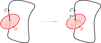
Figure 2: Infinitesimal opening of the closed contour ${\mathcal{C}}$ at the intersection point ${\mathcal{C}}{\hskip 0.50003pt{\,\cap\,}\hskip 0.50003pt}{\mathcal{V}}$.

To understand how Eq. (7) is equivalent to Eq. (5), consider a Wilson loop for a contour ${\mathcal{C}}$ that intersects with the coboundary ${\mathcal{V}}$ exactly once, so $\operatorname{int}({\mathcal{C}},{\mathcal{V}}){\,=\,}1$. From Eq. (6), we see that this also means ${\mathcal{C}}$ links exactly once with ${\mathcal{S}}$, so $\operatorname{link}({\mathcal{C}},{\mathcal{S}}){\,=\,}1$. We then find that the Wilson loop transforms as

$$\begin{split}W_{\rho}({\mathcal{C}})\,\,\mapsto\,\,&\lim_{{\mathcal{C}}^{\prime}\to\hskip 0.70004pt{\mathcal{C}}}\operatorname{tr}_{\rho}\bigg{[}\hskip 1.00006pt{\mathrm{P}\kern-1.00006pt\exp\bigg{(}\hskip 0.50003pt{\int_{{\mathcal{C}}^{\prime}}{\Omega}^{-1}{A}\hskip 1.00006pt{\Omega}+\Omega^{-1}d\Omega}\bigg{)}}\bigg{]}\,,\\ =\,\,&\lim_{{\mathcal{C}}^{\prime}\to\hskip 0.70004pt{\mathcal{C}}}\operatorname{tr}_{\rho}\bigg{[}\hskip 1.00006pt{\Omega^{-1}({\mathcal{P}}_{-})\,\mathrm{P}\kern-1.00006pt\exp\bigg{(}\hskip 0.50003pt{\int_{{\mathcal{C}}^{\prime}}A}\bigg{)}\,\Omega({\mathcal{P}}_{+})}\hskip 0.50003pt\bigg{]}\,,\end{split}$$ (9)

where ${\mathcal{C}}^{\prime}$ is nearly identical to ${\mathcal{C}}$ except that it has been infinitesimally “cut open” in the vicinity of ${\mathcal{V}}$ such that $\partial{\mathcal{C}}^{\prime}={\mathcal{P}}_{+}-{\mathcal{P}}_{-}$, as depicted in Fig. 2. Cyclically permuting the terms inside the trace, we find that the Wilson loop transforms as

$$\begin{split}W_{\rho}({\mathcal{C}})\,\,\mapsto\,\,\lim_{{\mathcal{C}}^{\prime}\to\hskip 0.70004pt{\mathcal{C}}}\operatorname{tr}_{\rho}\bigg{[}\hskip 1.00006pt{{\alpha}\,\mathrm{P}\kern-1.00006pt\exp\bigg{(}\hskip 0.50003pt{\int_{{\mathcal{C}}^{\prime}}A}\bigg{)}}\bigg{]}\hskip 1.00006pt=\,{\rho}({\alpha})\hskip 1.00006ptW_{\rho}({\mathcal{C}})\,,\end{split}$$ (10)

where $\rho(\alpha)$ enters with a single power because $\operatorname{int}({\mathcal{C}},{\mathcal{V}}){\,=\,}1$. As a result, we find that Eq. (10) is precisely the desired transformation of the Wilson loop for $\operatorname{link}({\mathcal{C}},{\mathcal{S}}){\,=\,}\operatorname{int}({\mathcal{C}},{\mathcal{V}})$ ${\,=\,}1$. When generalized to arbitrary linking number, the above calculation establishes the one-form symmetry transformation law for Wilson loops defined in Eq. (5).

The astute reader will notice that it was essential that the mismatch in the twisted gauge transformation is valued in a center element ${\alpha}{\,\in\,}Z(G)$, to make the symmetry operator topological. Otherwise, the branch cut ${\mathcal{V}}$ cannot be arbitrarily chosen, since $W_{\rho}({\mathcal{C}})$ will transform differently under $\Omega$ depending on precisely where ${\mathcal{C}}$ has been cut open to yield ${\mathcal{C}}^{\prime}$. In other words, if $\alpha$ were an arbitrary group element, its placement in the Wilson loop would matter and thus the corresponding transformation would not be topological.

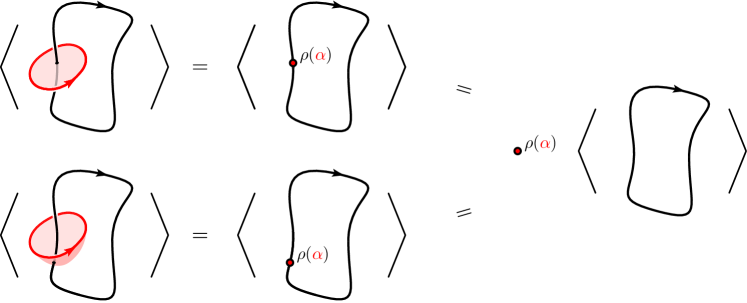
Figure 3: The one-form symmetry operator essentially inserts ${\rho}({\alpha})$ into the trace of the Wilson loop, where ${\alpha}{\,\in\,}Z(G)$ is a center element. The location of this insertion can be arbitrary since ${\alpha}$ commutes with all elements of $G$.

Before moving on, let us comment on a likely point of confusion. We have implemented the one-form symmetry transformation using a twisted gauge transformation $\Omega$ that is multivalued with a discontinuity center-valued in ${\alpha}$. However, we saw earlier that the symmetry operator $U_{\alpha}({\mathcal{S}})$ that implements this transformation should be labeled solely by the center element ${\alpha}$ rather than a whole zero-form parameter $\Omega$. Why does the twisted gauge transformation depend on $\Omega$ rather than just its twist ${\alpha}$? The resolution to this puzzle is that the naive $\Omega$ dependence in the twisted gauge transformation is spurious. Since $U_{\alpha}({\mathcal{S}})$ is a topological surface operator, it only links with one-dimensional objects. The only such gauge invariant objects are Wilson loops, and we have already shown that the action of the twisted gauge transformation on Wilson loops only depends on the center element ${\alpha}$, and not the details of $\Omega$. Hence, different choices of $\Omega$ which have the same twist valued in ${\alpha}$ are physically indistinguishable. In other words, symmetry operator is gauge invariant despite the appearance of a reference structure $\Omega$.

2.1.2 Ward Identity

Next, let us now derive the Ward identity which encodes the interplay between the symmetry operator $U_{\alpha}({\mathcal{S}})$ and the line operator $W_{\rho}({\mathcal{C}})$. Our goal is to prove that

$$\big{\langle}\hskip 0.50003pt{U_{\alpha}({\mathcal{S}})\hskip 1.00006ptW_{\rho}({\mathcal{C}})}\hskip 0.50003pt\big{\rangle}={\rho}({\alpha})^{\operatorname{link}({\mathcal{C}},{\mathcal{S}})}\big{\langle}\hskip 0.50003pt{W_{\rho}({\mathcal{C}})}\hskip 0.50003pt\big{\rangle}\,,$$ (11)

where the brackets denote the path integral over all fields, so for example

$$\big{\langle}\hskip 0.50003pt{U_{\alpha}({\mathcal{S}})\hskip 1.00006ptW_{\rho}({\mathcal{C}})}\hskip 0.50003pt\big{\rangle}=\int\mathcal{D}{A}\,\mathcal{D}{B}\,\,e^{-S}\,U_{\alpha}({\mathcal{S}})\,W_{\rho}({\mathcal{C}})\,.$$ (12)

Obviously, Eq. (11) is simply the transformation law for Wilson loops in Eq. (5), expressed in the language of covariant path integrals.

Earlier, we asserted that the one-form symmetry transformation in Eq. (5) is equivalent to the twisted gauge transformation defined in Eq. (7). The latter is implemented by the symmetry operator, which can be written in the explicit form,

$$U_{\alpha}({\mathcal{S}})=\exp\bigg{(}\hskip 1.00006pt{\frac{2\pi}{g^{2}}\int_{{\mathcal{S}}}\lambda^{a}\hskip 0.50003ptB_{a}}\bigg{)}\qquad\resizebox{}{}{\scalebox{0.95}[0.95]{{\leavevmode\hbox{\set@color{\text{where}}}}}}\qquad e^{2\pi\lambda}={\alpha}\in Z(G)\,,$$ (13)

where $\lambda^{a}$ is an adjoint-valued zero-form. Our claim is that the Ward identity in Eq. (11) follows mechanically from the definition of the line and symmetry operators in Eqs. (3) and (13), and furthermore we can see directly how the one-form symmetry transformation arises as a twisted gauge transformation. As before, the physical interpretation of Eq. (13) is that it inserts a Dirac string or vortex Reinhardt:2002mb ; Engelhardt:1999xw ; tHooft:1977nqb into spacetime. Note that Eq. (13) is a generalization of the center symmetry operator described in Gomes:2023ahz , which utilized temporal winding, and is also a special case of the family of symmetry operators constructed in Cordova:2022rer .

The definition of $U_{\alpha}({\mathcal{S}})$ in Eq. (13) may appear strange since the right-hand side is not manifestly a function of just the center element ${\alpha}$. Rather, it depends on a color reference $\lambda$ which has been chosen to exponentiate to ${\alpha}$. Even worse, $\lambda$ seems to specify an arbitrary vector in color space that naively violates gauge invariance. However, exactly like we saw for the twisted gauge transformation, the dependence on $\lambda$ is actually spurious. The properties of $U_{\alpha}({\mathcal{S}})$ are dictated entirely by its action on Wilson loops, which we will see depends only on ${\alpha}$. Hence, any distinct choices of $\lambda$ with the same twist ${\alpha}$ are physically equivalent. We will see this borne out explicitly in the subsequent calculation.

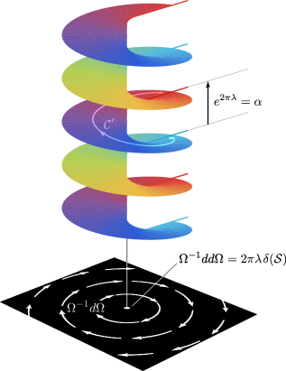
Figure 4: The twist of the multivalued gauge transformation can be characterized by the “curl” $\Omega^{-1}dd\Omega$ of the flat connection $\Omega^{-1}d\Omega$, which localizes along ${\mathcal{S}}$.

The proof of the Ward identity is as follows. To begin, we apply the twisted gauge transformation defined in Eq. (7), under which the field strength becomes

$$F^{a} \,\,\mapsto\,\,({\Omega}^{-1}{F}\hskip 1.00006pt{\Omega})^{a}+(\Omega^{-1}dd\Omega)^{a}\,.$$ (14)

As noted earlier, $dd\Omega=0$ everywhere that $d\Omega$ is well-defined. However, there are regions of spacetime where it is ill-defined. Again, this is analogous to $d\phi$ in polar coordinates, which is closed, not exact, and ill-defined at the origin. Furthermore, it can be illuminating to consider a distributional interpretation of $dd\phi$ which has nontrivial delta function support at precisely at the origin, so the integral of it over a disc yields $\int_{D^{2}}dd\phi=\int_{S^{1}}d\phi=2\pi$.

Similarly, for the case of our twisted gauge transformation, $dd\Omega$ has localized support on the surface ${\mathcal{S}}$ so in particular

$$(\Omega^{-1}dd\Omega)^{a}=2\pi\lambda^{a}\hskip 1.00006pt\delta({{\mathcal{S}}})\qquad\resizebox{}{}{\scalebox{0.95}[0.95]{{\leavevmode\hbox{\set@color{\text{for any $\lambda^{a}$ such that}}}}}}\qquad e^{2\pi\lambda}={\alpha}\in Z(G)\,.$$ (15)

Here $\delta({\mathcal{S}})$ is the two-form generalization of the Dirac delta distribution that peaks on ${\mathcal{S}}$ witten230b ; Gukov:2006jk , whose defining feature is that

$$\int_{\mathcal{M}}\varphi\wedge\delta({\mathcal{S}})=\int_{{\mathcal{S}}}\varphi\,,$$ (16)

for any two-form $\varphi$ in ${\mathcal{M}}$.

The equivalence between Eq. (8) and Eq. (15) can be understood intuitively from the visualization given in Fig. 4. The multivaluedness condition in Eq. (8) implies that the “gradient” $\Omega^{-1}d\Omega$ swirls about ${\mathcal{S}}$, and in turn, its “curl” $\Omega^{-1}dd\Omega$ localizes along ${\mathcal{S}}$ as a delta function, describing a Dirac string. A proof of this equivalence is left to App. B, which is essentially a colored generalization of our simpler example $dd\phi=2\pi\hskip 1.00006pt\delta(x)\hskip 0.50003pt\delta(y)\hskip 1.00006ptdx{\hskip 1.00006pt{\wedge}\,}dy$. We will also provide explicit examples of $\Omega$ later on.

With this understanding, we observe that that Eq. (13) can be written as

$$U_{\alpha}({\mathcal{S}})=\exp\bigg{(}\hskip 1.00006pt{\frac{1}{g^{2}}\int_{{\mathcal{M}}}B_{a}\wedge 2\pi\lambda^{a}\delta({\mathcal{S}})}\bigg{)}=\exp\bigg{(}\hskip 1.00006pt{\frac{1}{g^{2}}\int_{{\mathcal{M}}}B_{a}\wedge(\Omega^{-1}dd\Omega)^{a}}\bigg{)}\,,$$ (17)

from which we can now revisit the left-hand side of the Ward identity in Eq. (12). The factor involving the action and the symmetry operator combine to give

$$e^{-S}\,U_{\alpha}({\mathcal{S}})=\exp\bigg{(}{-\frac{1}{g^{2}}\int_{\mathcal{M}}B_{a}\wedge(F{\,-\,}\Omega^{-1}dd\Omega)^{a}-\frac{1}{2}\hskip 1.00006ptB_{a}{\hskip 1.00006pt{\wedge}\,}{*}B^{a}}\hskip 1.00006pt\bigg{)}\,.$$ (18)

The twisted gauge transformation of the field strength in Eq. (14) eats up the $\Omega^{-1}dd\Omega$ term and absorbs the symmetry operator into the action, so

$$e^{-S}\,U_{\alpha}({\mathcal{S}})\,\,\mapsto\,\,e^{-S}\,.$$ (19)

Combing Eq. (5) and Eq. (19), we see that the left-hand side of the Ward identity in Eq. (12) transforms to

$$\begin{split}\big{\langle}\hskip 0.50003pt{U_{\alpha}({\mathcal{S}})\hskip 1.00006ptW_{\rho}({\mathcal{C}})}\hskip 0.50003pt\big{\rangle}\;\mapsto\;\int\mathcal{D}{A}\,\mathcal{D}{B}\,\,e^{-S}\hskip 1.00006pt{\rho}({\alpha})^{\operatorname{link}({\mathcal{C}},{\mathcal{S}})}\hskip 1.00006ptW_{\rho}({\mathcal{C}})\,,\end{split}$$ (20)

which proves the Ward identity in Eq. (11).

In summary, Eqs. (7) and (15) specify a change of field variables that absorbs the symmetry operator into the action as Eq. (19). Note that Eq. (19) clearly shows the action is not invariant under Eq. (7), as the Lagrangian four-form in Eq. (2) changes on the support of the surface ${\mathcal{S}}$. Hence we learn again explicitly that Eq. (7) is not a typical gauge transformation in Yang-Mills theory, which would leave the Lagrangian four-form at all points in spacetime invariant. Of course, if we excise the region ${\mathcal{S}}$ from spacetime, then the twisted gauge transformation in Eq. (7) becomes a bona fide gauge transformation in the resulting punctured manifold, as mentioned earlier in our discussion of Maxwell theory.

A few more remarks are in order. Firstly, it should be clear from the above logic that the twisted gauge transformation in Eq. (7) describes the action of the one-form symmetry operator $U_{\alpha}({\mathcal{S}})$ on arbitrary operators. That is, if the twisted gauge transformation sends an operator ${\cal O}$ to ${\cal O}_{\Omega}$, then there is a corresponding generalized Ward identity,

$$\begin{split}\big{\langle}\hskip 0.50003pt{U_{\alpha}({\mathcal{S}})\hskip 1.00006pt{\cal O}}\hskip 0.50003pt\big{\rangle}&=\big{\langle}\hskip 0.50003pt{{\cal O}_{\Omega}}\hskip 0.50003pt\big{\rangle}\,,\end{split}$$ (21)

reiterating the fact that the one-form symmetry operator bridges between different center-twisted topological sectors of the gauge bundle. In fact, the Ward identity of Wilson loops in Eq. (11) can be regarded as a corollary of Eq. (21). Also, although Eq. (21) applies to local operators, it should be understood that any such point-supported operator is actually invariant under the one-form symmetry because the twisted gauge transformation can always be locally untwisted by a conventional gauge transformation. Geometrically, this reflects the fact that a point does not link with a codimension two object.

Secondly, the derivation of the Ward identity turns out to be very simple in the case of Maxwell theory with an exact contour ${\mathcal{C}}$. In this case the Wilson loop can be rewritten as a surface integral of the field strength $F$, as is familiar from the computation of the Aharonov-Bohm phase of a particle induced by a magnetic flux. The twisted gauge transformation of the field strength in Eq. (14) then creates a localized flux tube on the support of ${\mathcal{S}}$ whose integral over the surface yields the desired linking number. This is consistent with the above proof through a duality in the linking number computation described in App. B.

Thirdly, let us elaborate on the group multiplication rule for the symmetry operator, $U_{{\alpha}_{1}}({\mathcal{S}})\hskip 1.00006ptU_{{\alpha}_{2}}({\mathcal{S}})=U_{{\alpha}_{1}{\alpha}_{2}}({\mathcal{S}})$, which is required axiomatically. Since our symmetry operator implements a twisted gauge transformation, the composition of two such transformations automatically yields a third, so we know a priori that the group composition law is valid. However, establishing this more directly in terms of the expression in Eq. (13) is more subtle. In particular, suppose $U_{{\alpha}_{1}}({\mathcal{S}})$ and $U_{{\alpha}_{2}}({\mathcal{S}})$ are realized with the color reference vectors $\lambda_{1}$ and $\lambda_{2}$. The product $U_{{\alpha}_{1}}({\mathcal{S}})\hskip 1.00006ptU_{{\alpha}_{2}}({\mathcal{S}})$ naively exponentiates to symmetry operator with the color reference vector $\lambda_{1}{\,+\,}\lambda_{2}$, which confusingly is not guaranteed to exponentiate to a center element in general. However, this puzzle is resolved by realizing that $\lambda_{1}{\,+\,}\lambda_{2}$ would correspond to a twisted gauge transformation with an irrational period. As described at length in Sec. 2.1.1 and in Fig. 3, the periods of the twisted gauge transformations must be center-valued in order for the symmetry operator to be topological. Otherwise line operators will not transform correctly.

In order to properly implement sequential twisted gauge transformations, the representative Lie algebra elements for $U_{{\alpha}_{1}}({\mathcal{S}})$ and $U_{{\alpha}_{2}}({\mathcal{S}})$ can be chosen as

$${\alpha}_{1}=e^{2\pi\hskip 0.70004pt{\Omega_{2}}^{-1}\lambda_{1}\Omega_{2}}\qquad\resizebox{}{}{\scalebox{0.95}[0.95]{{\leavevmode\hbox{\set@color{\text{and}}}}}}\qquad{\alpha}_{2}=e^{2\pi\lambda_{2}}\,.$$ (22)

These color references merge into a new one, ${\Omega_{2}}^{-1}\lambda_{1}\hskip 0.50003pt\Omega_{2}+\lambda_{2}$, which corresponds to the desired composite twisted gauge transformation,

$$\begin{split}\Omega=\Omega_{1}\Omega_{2}{\quad\implies\quad}\Omega^{-1}dd\Omega\hskip 1.00006pt&=\hskip 1.00006pt2\pi({\Omega_{2}}^{-1}\lambda_{1}\hskip 0.50003pt\Omega_{2}+\lambda_{2})^{a}\hskip 1.00006pt\delta({\mathcal{S}})\,.\end{split}$$ (23)

This establishes the group composition law. In summary, the topological nature and gauge invariance of the symmetry operator together implies that the representative Lie algebra elements for the center elements in the group composition equation should be chosen in a specific form such that the composability and closure of center-twisted gauge transformations are correctly realized.

Last but not least, we realize that the above derivation of the Ward identity implies a remarkably simple and universal recipe for deducing the symmetry operator directly from the action itself. In particular, starting from any “$BF\hskip 0.50003pt$”-type Lagrangian of the form $B_{a}{\hskip 1.00006pt{\wedge}\,}F^{a}+f(B)$, we can define the symmetry operator as the object which is generated by a twisted gauge transformation. While the one-form symmetry operator is exactly eliminated by a twisted gauge transformation of the action, the $f(B)$ term will only serve as a spectator. This observation indeed is the key insight that will allow us to identify an explicit a one-form symmetry operator for gravity in Sec. 3.

2.1.3 Explicit Examples

As summarized in Eq. (21), the one-form symmetry of Yang-Mills theory is implemented by a twisted gauge transformation $\Omega$ that winds nontrivially with a mismatch valued in the center element ${\alpha}{\,\in\,}Z(G)$. In this section, we will explicitly construct some examples of $\Omega$ and apply them to various classical backgrounds. The resulting twisted backgrounds will reveal some illuminating physical interpretations for the one-form symmetry operator itself. For concreteness, we specialize in gauge group $G=\mathrm{SU}(N)$, whose center is $Z(G)=\mathbb{Z}_{N}$.

Symmetry Operator as Thin Solenoid

Suppose the spacetime is flat Euclidean space ${\mathcal{M}}=\mathbb{R}^{4}$, equipped with Cartesian coordinates $x^{\mu}=(x,y,z,t)$. Consider a twisted gauge transformation,

$$\Omega=\exp\bigg{(}\hskip 0.50003pt{\frac{k}{N}\hskip 1.00006ptc\hskip 1.00006pt\phi}\hskip 0.50003pt\bigg{)}\qquad\resizebox{}{}{\scalebox{0.95}[0.95]{{\leavevmode\hbox{\set@color{\text{where}}}}}}\qquad e^{2\pi c}={\hbox to0.0pt{1\hss}\hskip 1.6pt\resizebox{}{}{\scalebox{1.1}[1.1]{{\leavevmode\hbox{\set@color{1}}}}}}\,,$$ (24)

where $\phi$ is the azimuthal angle such that $\tan\phi=y/x$, and $k$ is an integer. Here we have defined $c$ to be an element of the Lie algebra of ${\mathrm{SU}}(N)$ that exponentiates to the identity via $e^{2\pi c}={\hbox to0.0pt{1\hss}\hskip 1.6pt\resizebox{}{}{\scalebox{1.1}[1.1]{{\leavevmode\hbox{\set@color{1}}}}}}$, so in the fundamental representation we might have Gomes:2023ahz

$$c^{i}{}_{j}\hskip 1.00006pt=\hskip 1.00006pti\hskip 1.00006pt\operatorname{diag}(1,1,\cdots,-N{\hskip 1.00006pt+\hskip 1.00006pt}1)\,,$$ (25)

where $i,j,\ldots$ denote fundamental indices.

To demonstrate the transformation, let us consider a trivial background corresponding to $A^{a}{\,=\,}0$, $B_{a}{\,=\,}0$, where all the Wilson loops are trivial as $W_{\rho}({\mathcal{C}}){\,=\,}\dim{\rho}$, in particular $W_{\text{fund}}({\mathcal{C}}){\,=\,}N$ for the fundamental representation. However, applying Eqs. (7) and (14) on this trivial background with $\Omega$ in Eq. (24), we obtain a nontrivial background,

$$\begin{split}A^{a}&=(\Omega^{-1}d\Omega)^{a}=\frac{k}{N}\hskip 1.00006ptc^{a}\hskip 1.00006ptd\phi=\frac{k}{N}\hskip 1.00006ptc^{a}\hskip 1.00006pt\frac{x\hskip 1.00006ptdy{\,-\,}y\hskip 1.00006ptdx}{x^{2}+y^{2}}\\ F^{a}&=(\Omega^{-1}dd\Omega)^{a}=\frac{k}{N}\hskip 1.00006ptc^{a}\hskip 1.00006ptdd\phi=\frac{k}{N}\hskip 1.00006pt2\pi c^{a}\hskip 1.00006pt\delta(x)\hskip 0.50003pt\delta(y)\hskip 1.00006ptdx{\hskip 1.00006pt{\wedge}\,}dy\,,\end{split}$$ (26)

with $B_{a}=0$ still vanishing. For instance, consider a contour ${\mathcal{C}}$ that loops the $z$-axis once. Then the Wilson loop for ${\mathcal{C}}$, in the fundamental representation, is given by

$$\operatorname{tr}_{\text{fund}}\mathrm{P}\kern-1.00006pt\exp\bigg{(}{\frac{k}{N}\hskip 1.00006ptc\int_{0}^{2\pi}\kern-1.99997ptd\phi}\hskip 0.50003pt\bigg{)} =e^{2\pi ik/N}N\,,$$ (27)

in the twisted background described in Eq. (26). This demonstrates how the one-form symmetry transformation on Wilson loops arise from a twisted gauge transformation.

Interestingly, from the field strength in Eq. (26) we see that the resulting twisted field configuration describes a line of color flux flowing through the $z$-axis for all times $t$. Hence, we conclude that the physical interpretation of $\Omega$ is that it spontaneously excites an infinitely thin, straight and static solenoid from the vacuum. In turn, this implies that the one-form symmetry operator inserts a colored Dirac string into spacetime. With this interpretation, the Ward identity in Eq. (11) can be understood as the measurement of the Aharonov-Bohm phase by the Wilson loop in the background of the Dirac string. Each time the Wilson loop winds about this thin solenoid, we accrue an additional phase factor of $e^{2\pi ik/N}$, describing the center twist represented as a complex phase in the fundamental representation:

$$(\hskip 1.00006pt{\Omega(\phi{\,=\,}2\pi)\hskip 1.00006pt\Omega^{-1}(\phi{\,=\,}0)})^{i}{}_{j}\hskip 1.00006pt=\hskip 1.00006pte^{2\pi ik/N}\hskip 1.00006pt\delta^{i}{}_{j}\,.$$ (28)

A few remarks are in order. Firstly, it is worth noting that in Eq. (24) we can shift $k$ by $pN$ for $p{\,\in\,}\mathbb{Z}$, and this realizes various solenoids of different “strengths” but all yielding the same monodromy. This is an instantiation of a comment made earlier, which is that different $\Omega$ can realize the same ${\alpha}$. Note also that a shift by $pN$ can be implemented by a gauge transformation which is not continuously connected to the identity.

Secondly, since the linking between line and symmetry operators is topological, all of our results must be insensitive to homeomorphic deformations of their corresponding integration surfaces. For this reason it is an amusing check to consider the twisted gauge transformation for a static but “wiggly” Dirac string,

$$\Omega=\exp\bigg{(}\hskip 1.00006pt{\frac{k}{N}\hskip 1.00006ptc\hskip 1.00006pt\phi}\hskip 1.00006pt\bigg{)}\qquad\resizebox{}{}{\scalebox{0.95}[0.95]{{\leavevmode\hbox{\set@color{\text{where}}}}}}\qquad\tan\phi=\frac{y{\,-\,}Y(z)}{x{\hskip 1.00006pt-\hskip 0.50003pt}X(z)}\,,$$ (29)

where $X(z)$ and $Y(z)$ describe a static line in space that is not necessarily straight. Here a simple calculation shows that the discontinuity in the twisted gauge transformation $\Omega^{-1}dd\Omega$ is proportional to

$$\delta(x{\hskip 1.00006pt-}X(z))\hskip 1.00006pt\delta(y{\hskip 1.00006pt-}Y(z))\,d(x{\hskip 1.00006pt-}X(z)){\hskip 1.00006pt{\wedge}\,}d(y{\hskip 1.00006pt-}Y(z))\,,$$ (30)

which is a Dirac string that is not straight. It is obvious that the Aharonov-Bohm phase computed by the Ward identity is not modified by these wiggles. Going a step further, one can also promote the parameterization of the discontinuity to $X(z,t)$ and $Y(z,t)$ corresponding to time-dependent wiggles of the Dirac string. This case also accords with the general formula in Eq. (154).

In principle, the most general possible twisted gauge transformation can have a generator $c$ that varies across spacetime. This variation in color space is perfectly possible and should also not alter the monodromies as long as it is properly derived form a multivalued transformation in accordance with Eq. (15).

Finally, let us take stock of the physical interpretation of the above calculation. The linking number between $U_{\alpha}({\mathcal{S}})$ and $W_{\rho}({\mathcal{C}})$ is typically interpreted as the center electric flux $U_{\alpha}({\mathcal{S}})$ measured in the presence of the worldline of a colored particle given by $W_{\rho}({\mathcal{C}})$. Interestingly, here we arrive at a dual, but completely equivalent picture: instead, $W_{\rho}({\mathcal{C}})$ is the Aharonov-Bohm phase computed for a color Dirac string created by $U_{\alpha}({\mathcal{S}})$.

Yet, clearly we have been cavalier about the global topology of ${\mathcal{S}}$ while demonstrating this example. In particular, because the thin solenoid extends off to infinity, we have not actually stipulated whether or how ${\mathcal{S}}$ “winds back” to form a closed surface. However, importantly, ${\mathcal{S}}$ must be closed in order for $U_{\alpha}({\mathcal{S}})$ to be a topological operator. So why did the example of the solenoid yield the correct picture, despite the fact that the global structure of ${\mathcal{S}}$ was not specified?

Physically speaking, this setup yielded a sensible result because we effectively zoomed into a local region of ${\mathcal{S}}$ which links with ${\mathcal{C}}$ and measured the associated Aharanov-Bohm phase. That is, in the neighborhood of any point on ${\mathcal{S}}$, the surface appears as an infinite plane, and $\Omega$ is simply described by Eq. (24). As long as the Wilson loop does not deviate substantially from this region, the Aharanov-Bohm phase will be completely ignorant of how the ends of the flux tube reattach—or possibly even terminate—in some distant region. This is why we could obtain the correct transformation of the Wilson loop despite ignoring the global topology of ${\mathcal{S}}$.

Mathematically speaking, Eq. (24) should be understood as an expression for $\Omega$ in a certain patch on spacetime, which notably does not include the point at infinity. The details of “winding back” for the closure of ${\mathcal{S}}$ are contained in the charts for $\Omega$ which cover those other patches, which we have not defined explicitly. As a result, with the knowledge of $\Omega$ in a single patch, Wilson loops are explicitly computable only when restricted to regions in this patch.

Symmetry Operator as Time Monodromy

Another interesting example is Yang-Mills theory at finite temperature, described by a compact product manifold with compactified Euclidean time,

$${\mathcal{M}}={\mathcal{M}}_{3}\times\mathrm{S}^{1}\,,\quad t\,\,\sim\,\,t+\beta\,.$$ (31)

In addition to the trivial vacuum, there is an infinite set of gauge equivalence classes for the background gauge field. For example, consider

$$A^{a} =n\hskip 1.00006pt\frac{2\pi c^{a}}{\beta}\hskip 1.00006ptdt\qquad\resizebox{}{}{\scalebox{0.95}[0.95]{{\leavevmode\hbox{\set@color{\text{where}}}}}}\qquad n\in\mathbb{Z}\,.$$ (32)

In this background, Wilson loops winding about the thermal circle are trivial, as $e^{2\pi nc}={\hbox to0.0pt{1\hss}\hskip 1.6pt\resizebox{}{}{\scalebox{1.1}[1.1]{{\leavevmode\hbox{\set@color{1}}}}}}$. Meanwhile, consider the following twisted gauge transformation:

$$\Omega=\exp\bigg{(}\hskip 1.00006pt{\frac{2\pi kc}{N}\frac{t}{\beta}}\hskip 1.00006pt\bigg{)}\,.$$ (33)

This maps the background considered in Eq. (32) to

$$A^{a} =\bigg{(}{n{\,+\,}\frac{k}{N}}\bigg{)}\hskip 1.00006pt\frac{2\pi c^{a}}{\beta}\hskip 1.00006ptdt\,,$$ (34)

so the Wilson loops gain a nontrivial phase factor of $e^{2\pi ik/N}$ per each thermal circle. Hence, the symmetry operator has induced a monodromy in the time direction.

Note that Eqs. (32) and (34) can be obtained by identifying the ends of a flat gauge field configuration in ${\mathcal{M}}_{3}$ times an interval with a twisted boundary condition. An implementation of this construction in Lorentzian signature can be found in Gomes:2023ahz .

An interesting feature of this example which is absent from the previous one is that the Wilson loops do not generally admit a coboundary. That is, they can be closed but not exact. However, the construction of the one-form symmetry in terms of a multivalued gauge transformation still applies.

Again, in the more rigorous sense Eq. (33) should be taken as the specification of $\Omega$ in a certain patch, say a ball in ${\mathcal{M}}_{3}$ times $\mathrm{S}^{1}$. Then the surface support of the symmetry operator can reside at a time slice along the boundary of a large volume that goes beyond the ball.

Symmetry Operator as Circular Loop

In the examples considered thus far, the symmetry operator exhibited support on a surface ${\mathcal{S}}$ that has infinitely large extent in some direction, thus always leaving a worry that an explicit global definition of ${\mathcal{S}}$ as a closed surface is not given. For completeness, we would like to end with an example that explicitly shows how the surface support ${\mathcal{S}}$ can be finite.

Recall earlier how we constructed a static color Dirac string on the $z$-axis. The corresponding worldsheet extended infinitely in the $t$-$z$ plane, so ${\mathcal{S}}$ was infinite. Here we will temper ${\mathcal{S}}$ onto compact support in two steps. First, we will roll up the string in its spatial directions, yielding a closed circular loop of finite radius. Consequently, ${\mathcal{S}}$ will be spatially compact. Second, we will pinch off this loop in time by setting the size of this loop to be vanishing except for a finite duration, so ${\mathcal{S}}$ will be temporally compact as well.

In the first step of this construction, we consider a completely static system in toroidal coordinates, which foliate three-dimensional space according to a circular “reference ring” of radius $a$ in the $x$-$y$ plane. In particular, the coordinates $(\tau,\sigma,\phi)$ are defined by

$$\begin{split}x=\frac{a\sinh\tau}{\cosh\tau-\cos\sigma}\cos\phi\,,\quad y=\frac{a\sinh\tau}{\cosh\tau-\cos\sigma}\sin\phi\,,\quad z=\frac{a\sin\sigma}{\cosh\tau-\cos\sigma}\,,\end{split}$$ (35)

where $\phi$ is the azimuthal angle in the $x$-$y$ plane. Surfaces of fixed $\tau{\,\geq\,}0$ label concentric two-tori which enclose the reference ring, while surfaces of fixed $-\pi{\,<\,}\sigma{\,\leq\,}\pi$ label two-spheres which intersect the reference ring. Also, here we choose the branch cut for $\sigma$ such that the discontinuity at $\sigma=\pm\pi$ develops on the disc enclosed by the reference ring.

Crucially, we can think of $\sigma$ as an angular coordinate that winds like a solenoid about the reference ring. Thus we can let the twisted gauge transformation parameter be

$$\Omega=\exp\bigg{(}\hskip 1.00006pt{\frac{k}{N}\hskip 1.00006ptc\hskip 1.00006pt\sigma}\hskip 1.00006pt\bigg{)}\,,$$ (36)

which clearly induces a rephasing for any holonomy that wraps the reference ring. The branch cut resides on a volume ${\mathcal{V}}$ corresponding to the static disc enclosed by the reference ring. Its boundary then defines the surface ${\mathcal{S}}=\partial{\mathcal{V}}$, which is the reference ring itself, namely a static loop of radius $a$ in the $x$-$y$ plane. Furthermore, we see that $\Omega$ correctly approaches the identity at spatial infinity, simply because spatial infinity corresponds to $\sigma=0$ in toroidal coordinates.

In the second step, we allow for the radius of the reference ring to change with time. To allow for this, we define toroidal coordinates for each time slice in which the reference ring has a time-varying radius $a(t)$. For example, let us define $a(t)$ to smoothly increase from and decrease to zero within a time interval $t\in[t_{1},t_{2}]$. With this temporal modification, the surface ${\mathcal{S}}$ has finite support in both time and space.

Let us end with a final remark. In general, one typically wants to construct a twisted gauge transformation parameter $\Omega$ for an arbitrarily shaped surface ${\mathcal{S}}$ in an arbitrary manifold ${\mathcal{M}}$ with or without boundaries. How do we know that such an $\Omega$ always exists, given some choice of ${\mathcal{S}}$ and ${\mathcal{M}}$? In all of the examples above we started with $\Omega$ as an input and rather determined the surface ${\mathcal{S}}$ as an output.

Interestingly, we find that it is always possible to find an $\Omega$ with a given ${\mathcal{S}}$ and ${\mathcal{M}}$, on account of a closely analogous question in classical magnetostatics. That is, deducing $\Omega$ from ${\mathcal{S}}$ and ${\mathcal{M}}$ is mathematically identical to deducing the static magnetic field and potential of an electric current loop. To see why, imagine we are experimentalists who construct a loop of electrical line current $\mathbf{J}$, built to specification according to some arbitrary contour. On account of Ampère’s law, ${\nabla}{\hskip 0.50003pt\times\hskip 1.00006pt}\mathbf{H}=\mathbf{J}$, we can then deduce the magnetic field $\mathbf{H}$, or even just measure it. In regions away from the current, we can then reconstruct a magnetic scalar potential via $\mathbf{H}{\,=\,}{-\mathbf{\nabla}\Psi}$. If the manifold ${\mathcal{M}}$ is not closed, then we can make its boundary $\partial{\mathcal{M}}$ superconducting to enforce the boundary condition $\mathbf{H}_{\perp}{\hskip 0.50003pt=\,}0$, in which case $\Psi$ can be set to a constant over $\partial{\mathcal{M}}$ that we fix to zero. In this analogy, the electric current $\mathbf{J}$, the magnetic field $\mathbf{H}$, and the magnetic potential $\Psi$ each correspond to the Dirac string defined by $\Omega^{-1}dd\Omega$, the twisted gauge connection $\Omega^{-1}d\Omega$, and the “log” of the twisted gauge parameter $\Omega$, respectively .

2.2 Canonical Formalism

The one-form symmetry of gauge theory can also be understood from the complementary point of view of the Hamiltonian formalism. To this end, we will study Yang-Mills theory on a spacetime described by a product manifold ${\mathcal{M}}={\mathcal{M}}_{3}{\,\times\hskip 1.00006pt}\mathbb{R}$ equipped with coordinates $x^{\mu}=(x^{i},x^{4})$. In particular, we perform a $3{\,+\,}1$ decomposition in which $x^{i}$ denotes coordinates of the spatial three-manifold ${\mathcal{M}}_{3}$ and $x^{4}=t$ defines equal-time slices.

2.2.1 Phase Space

The first-order formulation of Yang-Mills theory is defined in Eq. (2). Writing out all indices explicitly, we obtain the Lagrangian,

$$\begin{split}\frac{1}{g^{2}}\hskip 1.00006pt\bigg{[}\hskip 1.00006pt{\frac{1}{2}\hskip 1.00006ptB_{a\mu\nu}\Big{(}\hskip 0.50003pt{\partial_{\rho}A^{a}{}_{\sigma}+{\textstyle\frac{1}{2}}\hskip 1.00006ptf^{a}{}_{bc}\hskip 1.00006ptA^{b}{}_{\rho}\hskip 1.00006ptA^{c}{}_{\sigma}}\Big{)}\hskip 1.00006pt\epsilon^{\mu\nu\rho\sigma}-\frac{1}{4}\hskip 1.00006ptB_{a\mu\nu}B^{a\mu\nu}}\hskip 1.00006pt\bigg{]}\,,\end{split}$$ (37)

where $\epsilon^{\mu\nu\rho\sigma}$ denotes the permutation symbol. Carrying out the $3{\,+\,}1$ decomposition and integrating out $B_{ai4}$, we immediately see that the dynamical coordinates on the phase space are $A^{a}{}_{i}$ together with their canonical conjugates,

$$E^{i}{}_{a}=\frac{1}{2}\hskip 1.00006ptB_{ajk}\hskip 1.00006pt\epsilon^{ijk}\,.$$ (38)

Their canonical commutation relations given by

$$\begin{split}[A^{a}{}_{i}(x),A^{b}{}_{j}(x^{\prime})]&=0\,,\\ [E^{i}{}_{a}(x),A^{b}{}_{j}(x^{\prime})]&=g^{2}\,\delta^{i}{}_{j}\,\delta^{b}{}_{a}\,\delta^{(3)}(x{\,-\,}x^{\prime})\,,\\ [E^{i}{}_{a}(x),E^{j}{}_{b}(x^{\prime})]&=0\,,\end{split}$$ (39)

where $x,x^{\prime}\in{\mathcal{M}}_{3}$ are points in the spatial manifold. Note that there is no imaginary unit here since we are in Euclidean signature. The phase space is also equipped with the Gauss constraint and a Hamiltonian, the details of which are not important for our purposes.

2.2.2 Ward Identity

In the language of the path integral, a one-form symmetry transformation is implemented through the insertion of a symmetry operator which wraps the line operator. In the operator formalism, however, this corresponds to a conjugation of the latter by the former. To see how this works in detail, consider a line operator $W_{\rho}({\mathcal{C}})$, where ${\mathcal{C}}$ is restricted to an equal-time slice, say at $t{\,=\,}0$. As before, we take the symmetry operator $U_{\alpha}({\mathcal{S}})$ to be supported on an exact surface ${\mathcal{S}}$ with an associated coboundary ${\mathcal{V}}$, so ${\mathcal{S}}=\partial{\mathcal{V}}$.

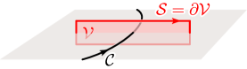
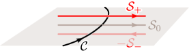
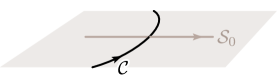
Figure 5: Pancaking the symmetry operator on a purely spatial line operator ${\mathcal{C}}$. The plane depicts an equal-time slice while time flows upwards. Top: The equal-time slice bisects the volume $\mathcal{V}$ by a surface ${\mathcal{S}}_{0}$. Middle: The surface ${\mathcal{S}}=\partial\mathcal{V}$ splits into surfaces ${\mathcal{S}}_{+}$ and $-{\mathcal{S}}_{-}$ at the infinitesimal future and past. Bottom: ${\mathcal{S}}_{+}$ and ${\mathcal{S}}_{-}$ both project down to the surface ${\mathcal{S}}_{0}$.

The geometric set-up is depicted in Fig. 5. We assume that the surface ${\mathcal{S}}$ links once with the purely spatial loop ${\mathcal{C}}$. Consequently, the coboundary ${\mathcal{V}}$ is intersected by the loop ${\mathcal{C}}$ and bisected by the spatial slice. Now imagine continuously squashing or pancaking the coboundary ${\mathcal{V}}$ along the time direction such that its two-dimensional boundary ${\mathcal{S}}$ infinitesimally hugs the spatial slice. In this limit, ${\mathcal{S}}={\mathcal{S}}_{+}{\hskip 1.00006pt\cup\hskip 1.00006pt}(-{\mathcal{S}}_{-})$ is the union of two disjoint discs ${\mathcal{S}}_{+}$ and $-{\mathcal{S}}_{-}$ at the infinitesimal future and past across $t{\,=\,}0$. Once ${\mathcal{V}}$ has completely collapsed into the spatial slice at $t{\,=\,}0$, both discs ${\mathcal{S}}_{\pm}$ approach the same surface, which we denote by ${\mathcal{S}}_{0}$. From Fig. 5, we see that this ${\mathcal{S}}_{0}$ will be the intersection between ${\mathcal{V}}$ and $t=0$. As a result, the intersection of ${\mathcal{C}}$ and ${\mathcal{V}}$ in the four-manifold ${\mathcal{M}}$ is equivalent to intersection of ${\mathcal{C}}$ and ${\mathcal{S}}_{0}$ in the three-manifold ${\mathcal{M}}_{3}$ as the slice $t{\,=\,}0$. Therefore, we have in general

$$\operatorname{link}({\mathcal{C}},{\mathcal{S}})\hskip 1.00006pt=\hskip 1.00006pt\operatorname{int}({\mathcal{C}},{\mathcal{V}})\hskip 1.00006pt=\hskip 1.00006pt\operatorname{int}_{3}({\mathcal{C}},{\mathcal{S}}_{0})\,,$$ (40)

where $\operatorname{int}_{3}$ denotes intersection number in ${\mathcal{M}}_{3}$.

Now, we can describe how this pancaking procedure boils down the Ward identity to an equal-time operator equation. Since ${\mathcal{S}}={\mathcal{S}}_{+}{\hskip 1.00006pt\cup\hskip 1.00006pt}(-{\mathcal{S}}_{-})$, we see that the symmetry operator factorizes into $U_{\alpha}({\mathcal{S}})=U_{\alpha}({\mathcal{S}}_{+})\hskip 1.00006ptU_{\alpha}(-{\mathcal{S}}_{-})$. In turn, the left-hand side of the Ward identity in Eq. (11) becomes the time-ordered expression $U_{\alpha}({\mathcal{S}}_{+})\hskip 1.00006ptW_{\rho}({\mathcal{C}})\hskip 1.00006ptU_{\alpha}(-{\mathcal{S}}_{-})$, which in the process of pancaking limits to the equal-time operator product $U_{\alpha}({\mathcal{S}}_{0})\hskip 1.00006ptW_{\rho}({\mathcal{C}})\hskip 1.00006ptU_{\alpha}\kern-3.00003pt\mathrlap{\leavevmode\hbox{\raise 1.1pt\hbox{\set@color\resizebox{}{}{{\leavevmode\hbox{\set@color{${}^{-1}$}}}}}}}\kern 9.49997pt({\mathcal{S}}_{0})$. Using Eq. (40), we then find that the Ward identity translates to

$$U_{\alpha}({\mathcal{S}}_{0})\,W_{\rho}({\mathcal{C}})\,U_{\alpha}\kern-3.00003pt\mathrlap{\leavevmode\hbox{\raise 1.1pt\hbox{\set@color\resizebox{}{}{{\leavevmode\hbox{\set@color{${}^{-1}$}}}}}}}\kern 9.49997pt({\mathcal{S}}_{0})\hskip 1.00006pt=\hskip 1.00006pt\rho(\alpha)^{\operatorname{int}_{3}({\mathcal{C}},{\mathcal{S}}_{0})}\,W_{\rho}({\mathcal{C}})\,,$$ (41)

which is an equal-time operator equation.

Eq. (41) is the avatar of the Ward identity in the operator formalism, where all the relevant geometric objects and operations, including the disc ${\mathcal{S}}_{0}$ and the closed contour ${\mathcal{C}}$, are defined within the three-manifold ${\mathcal{M}}_{3}$. The key insight here is that time ordering in the path integral formalism turns into operator ordering in the operator formalism.

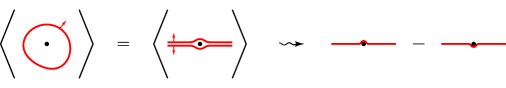
Figure 6: Zero-form version of the pancaking procedure, which the reader may be familiar with. Wrapping an operator with the symmetry operator translates to an equal-time conjugation, where operator ordering traces back to time ordering.

Finally, it is straightforward to explicitly evaluate Eq. (41). Applying the $3{\,+\,}1$ decomposition and using Eq. (38), the Hamiltonian formalism avatar of the symmetry operator, supported on a disc ${\mathcal{S}}_{0}{\,\subset\,}{\mathcal{M}}_{3}$ in three dimensions, is given as

$$U_{\alpha}({\mathcal{S}}_{0})=\exp\bigg{(}\hskip 1.00006pt{\frac{\pi}{g^{2}}\int_{{\mathcal{S}}_{0}}dx^{j}{\hskip 1.00006pt{\wedge}\,}dx^{k}\,\epsilon_{ijk}\hskip 1.00006ptE^{i}{}_{a}\hskip 1.00006pt\lambda^{a}}\bigg{)}\qquad\resizebox{}{}{\scalebox{0.95}[0.95]{{\leavevmode\hbox{\set@color{\text{where}}}}}}\qquad e^{2\pi\lambda}={\alpha}\,.$$ (42)

To compute $U_{\alpha}({\mathcal{S}}_{0})\hskip 1.00006ptW_{\rho}({\mathcal{C}})\hskip 1.00006ptU_{\alpha}\kern-3.00003pt\mathrlap{\leavevmode\hbox{\raise 1.1pt\hbox{\set@color\resizebox{}{}{{\leavevmode\hbox{\set@color{${}^{-1}$}}}}}}}\kern 9.49997pt({\mathcal{S}}_{0})$, let us first deduce how the conjugation acts on the phase space. While $E^{i}{}_{a}(x)$ is left invariant because $[E^{i}{}_{a}(x),E^{j}{}_{b}(x^{\prime})]=0$, the spatial gauge connection $A^{a}{}_{k}(x)$ has a nonvanishing commutator with the exponent of Eq. (42),

$$\begin{split}&\frac{\pi}{g^{2}}\hskip 1.00006pt\int_{{\mathcal{S}}_{0}}dx^{\prime i}{\hskip 1.00006pt{\wedge}\,}dx^{\prime j}\,\lambda^{b}(x^{\prime})\,\epsilon_{ijl}\hskip 1.00006pt[E^{l}{}_{b}(x^{\prime}),A^{a}{}_{k}(x)]\,\\ &\hskip 1.00006pt=\hskip 1.00006pt2\pi\int d\sigma_{1}\hskip 0.50003ptd\sigma_{2}\,\,\frac{\partial X^{i}}{\partial\sigma_{1}}\frac{\partial X^{j}}{\partial\sigma_{2}}\,\lambda^{a}(X)\,\epsilon_{ijk}\hskip 1.00006pt\delta^{(3)}(x-X)\,,\end{split}$$ (43)

where $(\sigma_{1},\sigma_{2})\mapsto X^{i}(\sigma_{1},\sigma_{2})$ is a parameterization of the surface ${\mathcal{S}}_{0}$. According to Eq. (154), this describes the components of the one-form $2\pi\lambda^{a}\hskip 1.00006pt\delta_{3}({\mathcal{S}}_{0})$, where $\delta_{3}({\mathcal{S}}_{0})$ is the Dirac delta one-form of ${\mathcal{S}}_{0}$ defined in the spatial three-manifold ${\mathcal{M}}_{3}$. Therefore, we can summarize the action of the symmetry transformation on the phase space variables as the following:

$$\begin{split}U_{\alpha}({\mathcal{S}}_{0})\,{A^{a}{}_{i}}\,U_{\alpha}\kern-3.00003pt\mathrlap{\leavevmode\hbox{\raise 1.1pt\hbox{\set@color\resizebox{}{}{{\leavevmode\hbox{\set@color{${}^{-1}$}}}}}}}\kern 9.49997pt({\mathcal{S}}_{0})&=(A^{a}+2\pi\lambda^{a}\hskip 1.00006pt\delta_{3}({\mathcal{S}}_{0}))_{i}\,,\\ U_{\alpha}({\mathcal{S}}_{0})\,{E^{i}{}_{a}}\,U_{\alpha}\kern-3.00003pt\mathrlap{\leavevmode\hbox{\raise 1.1pt\hbox{\set@color\resizebox{}{}{{\leavevmode\hbox{\set@color{${}^{-1}$}}}}}}}\kern 9.49997pt({\mathcal{S}}_{0})&=E^{i}{}_{a}\,.\end{split}$$ (44)

As a result, we find that the Wilson loop transforms as

$$\begin{split}U_{\alpha}({\mathcal{S}}_{0})\,W_{\rho}({\mathcal{C}})\,U_{\alpha}\kern-3.00003pt\mathrlap{\leavevmode\hbox{\raise 1.1pt\hbox{\set@color\resizebox{}{}{{\leavevmode\hbox{\set@color{${}^{-1}$}}}}}}}\kern 9.49997pt({\mathcal{S}}_{0})\hskip 1.00006pt=\hskip 1.00006pt\rho(\alpha)^{\operatorname{int}_{3}({\mathcal{C}},{\mathcal{S}}_{0})}\hskip 1.00006ptW_{\rho}(\mathcal{C})\,,\end{split}$$ (45)

which proves the Hamiltonian counterpart of the Ward identity. We have used the fact that the three-dimensional intersection number is is $\operatorname{int}_{3}({\mathcal{C}},{\mathcal{S}}_{0})=\oint_{\mathcal{C}}\delta_{3}({\mathcal{S}}_{0})$.

3 Gravity

Armed with an understanding of higher-form symmetry in gauge theory, we are now equipped to transcribe all of those results to the context of dynamical gravity. As is well-known, the tetradic Palatini formalism is a description of gravity in terms of a gauge theory of Lorentz transformations. Using this framework, we can deduce the higher-form symmetries of gravity by direct analogy. As before, we start with a covariant analysis and then describe the same physics using the canonical formalism.

3.1 Covariant Formalism

Consider dynamical gravity on a four-dimensional manifold ${\mathcal{M}}$ with Euclidean signature. As noted earlier, we work within the regime of validity of an effective field theory of gravity in which the topology and dimensionality of spacetime do not fluctuate.

Our point of departure is the tetradic Palatini formalism, which formulates gravity as a gauge theory of the four-dimensional Lorentz group $G$ and is inherently first-order. Here we emphasize again that despite our abuse of nomenclature we will consider both Lorentzian and Euclidean signature. The degrees of freedom are a one-form spin connection and one-form tetrad field,

$$\omega^{AB}=\omega^{AB}{}_{\mu}\hskip 1.00006ptdx^{\mu}\qquad\resizebox{}{}{\scalebox{0.95}[0.95]{{\leavevmode\hbox{\set@color{\text{and}}}}}}\qquad e^{A}=e^{A}{}_{\mu}\hskip 1.00006ptdx^{\mu}\,,$$ (46)

which transform in the adjoint and fundamental representation of $G$, so the uppercase indices are $A,B,\ldots\in\{1,2,3,4\}$.

In terms of these fields, the action for Palatini gravity is given by the integral over ${\mathcal{M}}$ of the Lagrangian four-form

$$L=\frac{1}{4g^{2}}\hskip 1.00006pt\epsilon_{ABCD}\hskip 1.00006pte^{A}{\hskip 1.00006pt{\wedge}\,}e^{B}{\hskip 1.00006pt{\wedge}\,}R^{CD}-\frac{\Lambda}{24g^{2}}\hskip 1.00006pt\epsilon_{ABCD}\hskip 1.00006pte^{A}{\hskip 1.00006pt{\wedge}\,}e^{B}{\hskip 1.00006pt{\wedge}\,}e^{C}{\hskip 1.00006pt{\wedge}\,}e^{D}\,,$$ (47)

where we have defined the Riemann curvature two-form,

$$R^{A}{}_{B}=d\omega^{A}{}_{B}+\omega^{A}{}_{C}{\hskip 1.00006pt{\wedge}\,}\omega^{C}{}_{B}\,,$$ (48)

which is simply the field strength for the spin connection. The first term in Eq. (47) encodes the Einstein-Hilbert Lagrangian, where we have repackaged Newton’s constant into $g=(8\pi G_{\text{N}})^{1/2}$ to draw a closer analogy with gauge theory. The second term in Eq. (47) defines the cosmological constant $\Lambda$.

It should be reiterated that both the spin connection and tetrad are taken as independent degrees of freedom in the tetradic Palatini formulation. To see how this approach reproduces conventional general relativity, let us vary the Lagrangian in Eq. (47) with respect to the spin connection and tetrad to obtain their respective equations of motion,

$$D(e^{A}{\hskip 1.00006pt{\wedge}\,}e^{B})=0\qquad\resizebox{}{}{\scalebox{0.95}[0.95]{{\leavevmode\hbox{\set@color{\text{and}}}}}}\qquad e^{[B}{\hskip 1.00006pt{\wedge}\,}R^{CD]}=\frac{\Lambda}{3}\hskip 1.00006pte^{B}{\hskip 1.00006pt{\wedge}\,}e^{C}{\hskip 1.00006pt{\wedge}\,}e^{D}\,,$$ (49)

where the square brackets on indices denote antisymmetrization. Here we have defined $D$ as the covariant exterior derivative with respect to the spin connection.

It is not difficult to show that the first equation of motion in Eq. (49) is algebraically equivalent to vanishing of $De^{A}=de^{A}+\omega^{A}{}_{B}{\hskip 1.00006pt{\wedge}\,}e^{B}$, which is the definition of torsion. This fixes the dynamics to be identically torsion-free. Any coupling of the spin connection to an external source generates nonzero torsion precisely only on the support of that source. Meanwhile, with vanishing torsion the second equation of motion in Eq. (49) becomes the Einstein field equations for the associated metric,

$$g_{\mu\nu}=\delta_{AB}\hskip 1.00006pte^{A}{}_{\mu}\hskip 1.00006pte^{B}{}_{\nu}\,.$$ (50)

As emphasized earlier, we work in an effective field theory description of gravity which describes gravitons propagating over a fixed background. Hence, throughout our analysis the metric and tetrad are implicitly expanded as fluctuations about some choice of background values $\bar{g}_{\mu\nu}$ and $\bar{e}^{A}{}_{\mu}$, respectively, though it will usually be simpler to manipulate the full field variables rather than their fluctuations.

Using integration by parts, it is easy to rewrite the Lagrangian in Eq. (47) so that it does not contain derivatives of the spin connection. Consequently, the spin connection is an auxiliary field that can be eliminated at tree-level by plugging in the classical solution for $\omega^{A}{}_{B}$ in terms of $e^{A}$ using the torsion-free condition in Eq. (49). The resulting Lagrangian, which depends solely on the tetrad, is precisely the usual Einstein-Hilbert Lagrangian. Therefore, tetradic Palatini gravity is classically equivalent to general relativity, provided there are no sources that couple directly to the spin connection so that torsion is vanishing. As noted earlier, quantum equivalence also follows, since the effective field theory of a massless spin two particle is unique, modulo Wilson coefficients.

Next, we would like to recall the well-known fact that tetradic Palatini gravity can be expressed in a way that even more directly parallels the first-order formulation of Yang-Mills theory. This fact will play a crucial role in our identification of the one-form symmetry later on. In particular, let us define the Plebański two-form Plebanski:1977zz ; Capovilla:1991qb by

$$B_{AB}=\frac{1}{2}\hskip 1.00006pt\epsilon_{ABCD}\hskip 1.00006pte^{C}{\hskip 1.00006pt{\wedge}\,}e^{D}\,,$$ (51)

which is valued in the adjoint of $G$. Expressed in terms of $B_{AB}$, the tetradic Palatini Lagrangian in Eq. (47) becomes

$$L=\frac{1}{g^{2}}\hskip 1.00006ptB_{a}{\hskip 1.00006pt{\wedge}\,}R^{a}-\frac{\Lambda}{6g^{2}}\hskip 1.00006ptB_{a}{\hskip 1.00006pt{\wedge}\,}{\star B}^{a}\,,$$ (52)

which is by construction identical in form to the Yang-Mills Lagrangian in Eq. (2). Here the lowercase indices $a,b,\ldots\in\{1,2,3,4,5,6\}$ transform in the adjoint of $G$, and $\star$ denotes the Hodge star in the internal Lorentz space, so when the adjoint indices are all converted to fundamental indices by the Lorentz algebra generator $(t_{a})^{A}{}_{B}$, we have

$$B_{AB}=\frac{1}{2}\hskip 1.00006pt\epsilon_{ABCD}\hskip 1.00006pte^{C}{\hskip 1.00006pt{\wedge}\,}e^{D}\qquad\resizebox{}{}{\scalebox{0.95}[0.95]{{\leavevmode\hbox{\set@color{\text{and}}}}}}\qquad{\star B}^{AB}=e^{A}{\hskip 1.00006pt{\wedge}\,}e^{B}\,.$$ (53)

We emphasize that $\star$ should be distinguished from $\ast$ in Eq. (2). Also, we clarify that fundamental indices $A,B,\cdots$ are raised and lowered by the Euclidean flat metric $\delta_{AB}$.

In terms of the Plebański two-form, the Lagrangian in Eq. (52), is clearly of the “$BF\hskip 0.50003pt$”-type Lagrangian of the form $B_{a}{\hskip 1.00006pt{\wedge}\,}F^{a}+f(B)$ which is familiar from gauge theory. Therefore, we can immediately identify the line operator and the symmetry operator for the one-form symmetry of gravity by essentially copying the formulae from our earlier discussion about Yang-Mills theory.

So what is the one-form symmetry of dynamical gravity? In analog with gauge theory, it is defined by the center of $G$, which is the four-dimensional Lorentz group. As usual, the center depends crucially on the global structure of $G$, which is not specified by the Lagrangian in Eq. (52). Therefore, it is essential to clarify the global structure of $G$ before we can continue further.

To begin, let us consider the case of Euclidean signature. Given the well-known Lie algebra isomorphism $\mathfrak{so}(4)\,\cong\,\mathfrak{su}(2){\hskip 1.00006pt\oplus\,}\mathfrak{su}(2)\,\cong\,\mathfrak{spin}(4)$, we can choose $G$ to be either

$$\mathrm{Spin}(4)\cong\mathrm{SU}(2){\hskip 1.00006pt\times\,}\mathrm{SU}(2)\qquad\resizebox{}{}{\scalebox{0.95}[0.95]{{\leavevmode\hbox{\set@color{\text{or}}}}}}\qquad\mathrm{SO}(4)\cong\frac{\mathrm{Spin}(4)}{\mathbb{Z}_{2}}\qquad\resizebox{}{}{\scalebox{0.95}[0.95]{{\leavevmode\hbox{\set@color{\text{or}}}}}}\qquad\frac{\mathrm{SO}(4)}{\mathbb{Z}_{2}}\cong\frac{\mathrm{Spin}(4)}{\mathbb{Z}_{2}{\hskip 1.00006pt\times\,}\mathbb{Z}_{2}}\,,$$ (54)

whose center subgroups are given by

$$\mathbb{Z}_{2}{\hskip 1.00006pt\times\,}\mathbb{Z}_{2}\qquad\resizebox{}{}{\scalebox{0.95}[0.95]{{\leavevmode\hbox{\set@color{\text{or}}}}}}\qquad\mathbb{Z}_{2}\qquad\resizebox{}{}{\scalebox{0.95}[0.95]{{\leavevmode\hbox{\set@color{\text{or}}}}}}\qquad{\hbox to0.0pt{1\hss}\hskip 1.6pt\resizebox{}{}{\scalebox{1.1}[1.1]{{\leavevmode\hbox{\set@color{1}}}}}}\,,$$ (55)

respectively. The one-form charges will be valued in these center subgroups. Note that the zero-form symmetry associated with the center $\mathbb{Z}_{2}{\hskip 1.00006pt\times\,}\mathbb{Z}_{2}$ of $\mathrm{Spin}(4)\cong\mathrm{SU}(2){\hskip 1.00006pt\times\,}\mathrm{SU}(2)$ acts as parity on chiral and antichiral spinor indices, while that of the center $\mathbb{Z}_{2}$ of $\mathrm{SO}(4)$ acts as parity on vector indices.

Meanwhile, in Lorentzian signature, possible candidates for the gauge group are

$$\mathrm{Spin}(3,1)\cong\mathrm{SL}(2,\mathbb{C})\qquad\resizebox{}{}{\scalebox{0.95}[0.95]{{\leavevmode\hbox{\set@color{\text{or}}}}}}\qquad\mathrm{SO}^{+}(3,1)\cong\frac{\mathrm{Spin}(3,1)}{\mathbb{Z}_{2}}\,,$$ (56)

where the latter is the orthochronous Lorentz group and the former is its double cover. The corresponding center subgroups are

$$\mathbb{Z}_{2}\qquad\resizebox{}{}{\scalebox{0.95}[0.95]{{\leavevmode\hbox{\set@color{\text{or}}}}}}\qquad{\hbox to0.0pt{1\hss}\hskip 1.6pt\resizebox{}{}{\scalebox{1.1}[1.1]{{\leavevmode\hbox{\set@color{1}}}}}}\,,$$ (57)

respectively, which define allowed one-form symmetry of gravity in Lorentzian signature. Here the zero-form symmetry associated with the former corresponds to net parity on chiral and antichiral spinor indices, also known as fermion parity.

Any choice of $G$ in Eq. (54) is viable. For the sake of generality, however, in the remainder of our analysis we will be agnostic and take the gauge group to be some general $G$ with center subgroup $Z(G)$.

3.1.1 Line and Symmetry Operators

We are now equipped to derive explicitly the one-form symmetry of dynamical gravity. As before, we start with identifying the line operator and its symmetry transformation.

Firstly, let us recall the direct parallel between the spin connection in Eq. (52) and the gauge connection in Eq. (2). As such, it is obvious that the natural line operator in gravity is the spin holonomy,

$$W_{\rho}({\mathcal{C}})=\operatorname{tr}_{{\rho}}\mathrm{P}\kern-1.00006pt\exp\bigg{(}\hskip 0.50003pt{\oint_{{\mathcal{C}}}\omega}\bigg{)}\,,$$ (58)

where ${\mathcal{C}}$ defines a closed one-dimensional contour and ${\rho}$ is some spin representation of the Lorentz group $G$. Far less clear a priori is the identity of the symmetry operator,

$$U_{\alpha}({\mathcal{S}})\,,$$ (59)

other than that it should be labeled by a center element ${\alpha}\in G$ and defined on an exact two-dimensional surface ${\mathcal{S}}=\partial{\mathcal{V}}$ that can topologically link with ${\mathcal{C}}$.

In perfect analogy with the Wilson loop of gauge theory, we expect that the spin holonomy should transform as

$$W_{\rho}({\mathcal{C}})\,\,\mapsto\,\,{\rho}({\alpha})^{\operatorname{link}({\mathcal{C}},{\mathcal{S}})}\hskip 1.00006ptW_{\rho}({\mathcal{C}})\,,$$ (60)

under the one-form symmetry of gravity, and this is indeed the case. As before, ${\operatorname{link}({\mathcal{C}},{\mathcal{S}})}$ is defined to be the linking number between the contour and surface that define the line and symmetry operators.

Mirroring Eq. (7) in gauge theory, the one-form symmetry of gravity is implemented as a transformation of the fields by a closed but not exact form. In the gravitational context, the appropriate map is a local Lorentz transformation that is multivalued. In particular, we consider the case where ${\mathcal{S}}=\partial{\mathcal{V}}$ and there is a branch cut on the coboundary ${\mathcal{V}}$ whose discontinuity is center-valued. Physically, this twisted Lorentz transformation boosts local laboratories in spacetime such that a $\pi$ rotation of frames is applied after each winding about ${\mathcal{S}}$. Specifically, the spin connection and the tetrad will transform as

$$\omega^{A}{}_{B} \,\,\mapsto\,\,(\Omega^{-1})^{A}{}_{C}\hskip 1.00006pt\omega^{C}{}_{D}\hskip 1.00006pt\Omega^{D}{}_{B}+(\Omega^{-1})^{A}{}_{C}\hskip 1.00006ptd\Omega^{C}{}_{B}\qquad\resizebox{}{}{\scalebox{0.95}[0.95]{{\leavevmode\hbox{\set@color{\text{and}}}}}}\qquad e^{A}\,\,\mapsto\,\,(\Omega^{-1})^{A}{}_{B}\,e^{B}\,,$$ (61)

from which the transformation of the Plebański two-form is given by

$$B^{A}{}_{B}\,\,\mapsto\,\,(\Omega^{-1})^{A}{}_{C}\hskip 0.50003ptB^{C}{}_{D}\hskip 1.00006pt\Omega^{D}{}_{B}\,,$$ (62)

where $\Omega$ is a multivalued zero-form which defines the twisted Lorentz transformation. Like in the case of gauge theory, $d\Omega$ is not exact because $\Omega$ carries winding. As before, we also impose a discontinuity condition across the branch cut, given by

$$\lim_{{\mathcal{P}}_{\pm}\to\,{\mathcal{P}}}\hskip 0.50003pt\Omega({\mathcal{P}}_{+})\hskip 1.00006pt\Omega^{-1}({\mathcal{P}}_{-})\,=\,{\alpha}\qquad\resizebox{}{}{\scalebox{0.95}[0.95]{{\leavevmode\hbox{\set@color{\text{where}}}}}}\qquad{\alpha}\in Z(G)\qquad\resizebox{}{}{\scalebox{0.95}[0.95]{{\leavevmode\hbox{\set@color{\text{and}}}}}}\qquad{\mathcal{P}}{\,\subset\,}{\mathcal{V}}\,,$$ (63)

where ${\mathcal{P}}_{+}$ and ${\mathcal{P}}_{-}$ are infinitesimally split across ${\mathcal{V}}$. In turn, it follows that the spin holonomy that links once with ${\mathcal{S}}$ maps to

$$\begin{split}W_{\rho}({\mathcal{C}})\,\,\mapsto\,\,&\lim_{{\mathcal{C}}^{\prime}\to\hskip 0.70004pt{\mathcal{C}}}\operatorname{tr}_{\rho}\bigg{[}\hskip 1.00006pt{\mathrm{P}\kern-1.00006pt\exp\bigg{(}\hskip 0.50003pt{\int_{{\mathcal{C}}^{\prime}}{\Omega}^{-1}{\omega}\hskip 1.00006pt{\Omega}+\Omega^{-1}d\Omega}\bigg{)}}\bigg{]}\,,\\ =\,\,&\lim_{{\mathcal{C}}^{\prime}\to\hskip 0.70004pt{\mathcal{C}}}\operatorname{tr}_{\rho}\bigg{[}\hskip 1.00006pt{\Omega^{-1}({\mathcal{P}}_{-})\,\mathrm{P}\kern-1.00006pt\exp\bigg{(}\hskip 0.50003pt{\int_{{\mathcal{C}}^{\prime}}\omega}\bigg{)}\,\Omega({\mathcal{P}}_{+})}\bigg{]}\\ =\,\,&\lim_{{\mathcal{C}}^{\prime}\to\hskip 0.70004pt{\mathcal{C}}}\operatorname{tr}_{\rho}\bigg{[}\hskip 1.00006pt{{\alpha}\,\mathrm{P}\kern-1.00006pt\exp\bigg{(}\hskip 0.50003pt{\int_{{\mathcal{C}}^{\prime}}\omega}\bigg{)}}\bigg{]}\,=\,{\rho}({\alpha})\hskip 1.00006ptW_{\rho}({\mathcal{C}})\,,\end{split}$$ (64)

which exactly instantiates Eq. (60). Thus, we conclude that the twisted local Lorentz transformation in Eq. (61) implements the gravitational one-form symmetry.

As in the gauge theory case, we emphasize here that $\Omega$ is not a bona fide gauge transformation when the center twist ${\alpha}$ is nontrivial. In particular, drawing an analogy with Eq. (15), we see that the double exterior derivative of $\Omega$ is nonzero,

$$(\Omega^{-1})^{A}{}_{C}\hskip 1.00006ptdd\Omega^{C}{}_{B}=2\pi\lambda^{A}{}_{B}\hskip 1.00006pt\delta({\mathcal{S}})\qquad\resizebox{}{}{\scalebox{0.95}[0.95]{{\leavevmode\hbox{\set@color{\text{for any $\lambda^{A}{}_{B}$ such that}}}}}}\qquad e^{2\pi\lambda}={\alpha}\in Z(G)\,,$$ (65)

and in fact has nonvanishing support precisely on ${\mathcal{S}}$.

Before continuing, let us address some possible confusions relating to Lorentz and diffeomorphism invariance. First of all, just like in Yang-Mills theory, we see here that the twisted Lorentz transformation depends on the whole function $\Omega$ rather than just ${\alpha}$. Naively, this dependence is Lorentz-violating, since $\Omega$ defines a trajectory in the space of Lorentz transformations. However, just as before, we can see that this dependence is spurious since different choices for $\Omega$ which exhibit the same twist ${\alpha}$ still act indistinguishably on the spin holonomy, and are thus physically equivalent.

Secondly, in the presence of dynamical gravitation there is a further caveat regarding the diffeomorphism invariance of the line operator $W_{\rho}({\mathcal{C}})$ and symmetry operator $U_{\alpha}({\mathcal{S}})$. Although these objects do not carry dangling indices, they do depend on a particular choice of a contour ${\mathcal{C}}$ and surface ${\mathcal{S}}$, which define collections of points in spacetime in the very same way that a local operator ${\cal O}(x)$ defines a single point. However, any local or quasi-local object such as a point, curve, or surface in spacetime is famously not diffeomorphism invariant, simply because “$x$” itself is not diffeomorphism invariant. Note that this annoyance is also implicitly present in any discussion of gauge theory Wilson loops in the presence of gravity, which is central to discussions of swampland conjectures. To address this, one typically appeals to the restoration of diffeomorphism invariance by “gravitationally dressing” Donnelly:2016rvo ; Giddings:2022hba the operator in question. A closely related tactic is to define all positions “relationally” in terms of some asymptotic reference, either at spatial infinity or the beginning of time.

However, diffeomorphism invariance is restored here in the very same way as Lorentz invariance. Since the linking number is itself diffeomorphism invariant, it means that operators related to each other by a diffeomorphism are themselves are physically equivalent.

3.1.2 Ward Identity

Next, let us compute the Ward identity associated with the gravitational one-form symmetry. Taking inspiration from Eq. (13) in the case of gauge theory, we define the one-form symmetry operator of gravity to be

$$U_{\alpha}({\mathcal{S}})=\exp\bigg{(}\hskip 1.00006pt{\frac{\pi}{g^{2}}\int_{{\mathcal{S}}}\hskip 1.00006pt\lambda^{AB}\hskip 0.50003ptB_{AB}}\bigg{)}\qquad\resizebox{}{}{\scalebox{0.95}[0.95]{{\leavevmode\hbox{\set@color{\text{where}}}}}}\qquad e^{2\pi\lambda}={\alpha}\in Z(G)\,,$$ (66)

where $\lambda$ is a zero-form function which is chosen so that at all points in spacetime it exponentiates to a center element of the Lorentz group. Again, this formula should be understood as a realization of the symmetry operator $U_{\alpha}({\mathcal{S}})$ with a representative Lie algebra element $\lambda$ for ${\alpha}$, as all choices of $\lambda$ with the same twist ${\alpha}$ act the same on the spin holonomy and are thus physically equivalent.

Intriguingly, this surface operator $U_{\alpha}({\mathcal{S}})$ literally computes a certain area-like quantity associated with ${\mathcal{S}}$! In particular, by reverting to tetrad variables and reintroducing Newton’s constant, we find that the symmetry operator is

$$U_{\alpha}({\mathcal{S}})=\exp\bigg{(}\hskip 1.00006pt{\frac{1}{4G_{\text{N}}}\int_{{\mathcal{S}}}\hskip 1.00006pt\frac{1}{2}\,{\star\lambda}_{AB}\hskip 1.00006pt(e^{A}{\hskip 1.00006pt{\wedge}\,}e^{B})}\hskip 1.00006pt\bigg{)}\,,$$ (67)

where ${\star\lambda}_{AB}=\frac{1}{2}\hskip 1.00006pt\epsilon_{ABCD}\hskip 1.00006pt\lambda^{CD}$ is the Hodge dual of $\lambda^{AB}$. Here we recognize $e^{A}{\hskip 1.00006pt{\wedge}\,}e^{B}$ as the infinitesimal area element in the orthonormal frame, so the exponent computes the area smeared with a reference $\star\lambda_{AB}$, measured in Planck units. Note that $1/2$ is the canonical normalization factor for contracting antisymmetric tensors.

Additionally, it is curious that the exponent in Eq. (67), or equivalently in Eq. (128), is tantalizingly similar to the area operator in loop quantum gravity which leads to the quantization of tetrahedral volume Rovelli:1994ge ; Ashtekar:1996eg . The only crucial difference is that here the area is “dotted” with a Lorentz generator $\lambda^{AB}$ that exponentiates to the center, so in a sense it serves as a discrete and topological reincarnation of the area operator in loop quantum gravity. On the other hand, $U_{\alpha}({\mathcal{S}})$ is also reminiscent of the Bekenstein-Hawking entropy formula Bekenstein:1973ur ; Hawking:1975vcx . Of course, these could easily be accidents of dimensional analysis on account of the $1/G_{\rm N}$ normalization in the exponent. But in any case, it would be fascinating to see if any of these superficial similarities carry deeper significance.

Meanwhile, a virtue of the algebra isomorphism $\mathfrak{so}(4)\cong\mathfrak{su}(2){\hskip 1.00006pt\oplus\,}\mathfrak{su}(2)$ is that we always can split the six generators of the Lorentz group $G$ into three chiral and three antichiral $\mathrm{SU}(2)$ generators. Assigning dotted and undotted spinor indices to each sector, we see that the spin connection decomposes into self-dual and anti-self-dual components, $\omega^{{\dot{\alpha}}{\dot{\beta}}}$ and $\omega^{\alpha\beta}$, while the tetrad is $e^{{\dot{\alpha}}\alpha}$. Similarly, the Plebański two-form $B_{a}$ decomposes into $B^{{\dot{\alpha}}{\dot{\beta}}}=\epsilon_{\alpha\beta}\hskip 1.00006pt(e^{{\dot{\alpha}}\alpha}{\hskip 1.00006pt{\wedge}\,}e^{{\dot{\beta}}\beta})$ and $B^{\alpha\beta}=-{\tilde{\epsilon}}_{\smash{{\dot{\alpha}}{\dot{\beta}}}\vphantom{\beta}}\hskip 1.00006pt(e^{{\dot{\alpha}}\alpha}{\hskip 1.00006pt{\wedge}\,}e^{{\dot{\beta}}\beta})$. See App. A for more details. Meanwhile, since the two $\mathfrak{su}(2)$ sectors commute, any element of the Lorentz algebra that exponentiates to a center element can be split into self-dual and anti-self-dual generators that separately exponentiate to center elements. Given these facts, we see that the symmetry operator decomposes into more primordial building blocks, which are chiral symmetry operators,

$$\begin{split}\widetilde{U}({\mathcal{S}})=\exp\bigg{(}{-\frac{1}{4G_{\text{N}}}\int_{{\mathcal{S}}}\hskip 1.00006pt\tilde{\lambda}^{\dot{\beta}}{}_{\dot{\alpha}}\,e^{{\dot{\alpha}}\alpha}{\hskip 1.00006pt{\wedge}\,}e_{\smash{\alpha{\dot{\beta}}}\vphantom{\beta}}}\hskip 1.00006pt\bigg{)}&\qquad\resizebox{}{}{\scalebox{0.95}[0.95]{{\leavevmode\hbox{\set@color{\text{where}}}}}}\qquad(e^{2\pi\tilde{\lambda}})^{\dot{\alpha}}{}_{\dot{\beta}}=-\delta^{\dot{\alpha}}{}_{\dot{\beta}}\,,\\ U({\mathcal{S}})=\exp\bigg{(}{-\frac{1}{4G_{\text{N}}}\int_{{\mathcal{S}}}\hskip 1.00006pt\lambda_{\alpha}{}^{\beta}\hskip 1.00006pte_{\smash{\beta{\dot{\alpha}}}\vphantom{\beta}}{\hskip 1.00006pt{\wedge}\,}e^{{\dot{\alpha}}\alpha}}\hskip 1.00006pt\bigg{)}&\qquad\resizebox{}{}{\scalebox{0.95}[0.95]{{\leavevmode\hbox{\set@color{\text{where}}}}}}\qquad(e^{2\pi\lambda})_{\alpha}{}^{\beta}=-\delta_{\alpha}{}^{\beta}\,.\end{split}$$ (68)

Here $\tilde{\lambda}^{\dot{\alpha}}{}_{\dot{\beta}}$ and $\lambda_{\alpha}{}^{\beta}$ belong to the self-dual and anti-self-dual Lie algebras.

For the case of Euclidean signature with $G=\mathrm{Spin}(4)$, the chiral operators $\widetilde{U}({\mathcal{S}})$ and $U({\mathcal{S}})$ are precisely the one-form symmetry operators corresponding to each factor of the center subgroup $Z(G)=\mathbb{Z}_{2}\times\mathbb{Z}_{2}$. Note that, as zero-form symmetries, each factor of the center acts as parity in the numbers of dotted and undotted spinor indices, respectively. In Lorentzian signature, however, the one-form symmetry is only nontrivial if $G=\mathrm{SL}(2,\mathbb{C})$, in which case the center subgroup is $Z(G)=\mathbb{Z}_{2}$. As a zero-form symmetry this acts as net parity on spinor indices. In this case, only the real combination of the chiral operators, $\widetilde{U}({\mathcal{S}})\hskip 1.00006ptU({\mathcal{S}})$, corresponds to the one-form symmetry operator.

Now let us finally present a derivation of the Ward identity associated with the one-form symmetry of gravity,

$$\big{\langle}\hskip 0.50003pt{U_{\alpha}({\mathcal{S}})\hskip 1.00006ptW_{\rho}({\mathcal{C}})}\hskip 0.50003pt\big{\rangle}={\rho}({\alpha})^{\operatorname{link}({\mathcal{C}},{\mathcal{S}})}\big{\langle}\hskip 0.50003pt{W_{\rho}({\mathcal{C}})}\hskip 0.50003pt\big{\rangle}\,.$$ (69)

Since the tetradic Palatini framework is a first-order formalism, the left-hand side is given by a path integral over all configurations of both the spin connection and the tetrad,

$$\big{\langle}\hskip 0.50003pt{U_{\alpha}({\mathcal{S}})W_{\rho}({\mathcal{C}})}\hskip 0.50003pt\big{\rangle}=\int\mathcal{D}{\omega}\,\mathcal{D}{e}\,\,e^{-S}\,U_{\alpha}({\mathcal{S}})\,W_{\rho}({\mathcal{C}})\,.$$ (70)

As before, the symmetry operator $U_{\alpha}({\mathcal{S}})$ merges with $e^{-S}$ to give

$$e^{-S}\,U_{\alpha}({\mathcal{S}})=\exp\bigg{(}{-\frac{1}{4g^{2}}\int_{\mathcal{M}}\epsilon_{ABCD}\hskip 1.00006pte^{A}{\hskip 1.00006pt{\wedge}\,}e^{B}\wedge(R-\Omega^{-1}dd\Omega)^{CD}+\ldots}\hskip 1.00006pt\bigg{)}\,,$$ (71)

in analogy with Eq. (18), and where the ellipses denote the cosmological constant term. Meanwhile, we see that the twisted Lorentz transformation in Eq. (61) implies

$$R^{A}{}_{B} \,\,\mapsto\,\,(\Omega^{-1})^{A}{}_{C}\hskip 1.00006ptR^{C}{}_{D}\hskip 1.00006pt\Omega^{D}{}_{B}+(\Omega^{-1})^{A}{}_{C}\hskip 1.00006ptdd\Omega^{C}{}_{B}\,,$$ (72)

which is gravitational analog of Eq. (14). Applying this to Eq. (71), we find

$$e^{-S}\,U_{\alpha}({\mathcal{S}})\,\,\mapsto\,\,e^{-S}\,.$$ (73)

Together with the transformation of the line operator in Eq. (60), Eq. (73) sends the left-hand side of the Ward identity in Eq. (70) to

$$\begin{split}\big{\langle}\hskip 0.50003pt{U_{\alpha}({\mathcal{S}})\hskip 1.00006ptW_{\rho}({\mathcal{C}})}\hskip 0.50003pt\big{\rangle}\;\mapsto\;\int\mathcal{D}{\omega}\,\mathcal{D}{e}\,\,e^{-S}\hskip 1.00006pt{\rho}({\alpha})^{\operatorname{link}({\mathcal{C}},{\mathcal{S}})}\hskip 1.00006ptW_{\rho}({\mathcal{C}})\,,\end{split}$$ (74)

which is precisely its right-hand side. This proves the Ward identity encoding the topological linking of the spin holonomy in Eq. (58) with the symmetry operator in Eq. (66).

Just like in the case of gauge theory, the one-form symmetry of gravity acts as a twisted Lorentz transformation on any choice of operator. Thus, if an operator transforms under the twisted Lorentz transformation as ${\cal O}\mapsto{\cal O}_{\Omega}$, then the corresponding Ward identity is $\big{\langle}\hskip 0.50003pt{U_{\alpha}({\mathcal{S}})\hskip 1.00006pt{\cal O}}\hskip 0.50003pt\big{\rangle}=\big{\langle}\hskip 0.50003pt{{\cal O}_{\Omega}}\hskip 0.50003pt\big{\rangle}$ in parallel with Eq. (21).

Before continuing, let us highlight an important point: the one-form symmetry of gravity is independent of our choice of formalism. In particular, while our derivations have made elaborate use of tetradic Palatini gravity, our final conclusions remain valid independent of this choice. For example, integrating out the spin connection yields a pure tetrad theory, but this still exhibits the one-form symmetry.

On the other hand, it is natural to ask about gravity in the pure metric formulation, where there is no tetrad, spin connection, or local Lorentz symmetry to speak of. In this case one formulates the dynamics only in terms of the metric, which is manifestly invariant under the twisted Lorentz transformation defined in Eq. (61), since $g_{\mu\nu}\mapsto g_{\mu\nu}$. Has the one-form symmetry disappeared? For the spinor holonomy, the answer is yes, but for the simple reason that we cannot even write it down since there is no tetrad field to characterize the gravitational interactions of fermions. This would be analogous to studying Yang-Mills theory with the stipulation that we can only ever use adjoint indices, thus precluding the existence of the very fundamental Wilson loops which are charged under the one-form symmetry. On the other hand, the vector holonomy and its one-form symmetry properties should presumably have a pure metric description since spin structure should not be necessary. Note that there has been some interesting recent work constructing continuous one-form symmetries of linearized gravity using the metric alone Hinterbichler:2022agn ; Benedetti:2021lxj ; Benedetti:2023ipt . It would be very illuminating to see explicitly how those symmetries relate to the ones derived in this paper.

3.1.3 Chiral Cosmic String

Just as in gauge theory, the one-form symmetry operator in gravity can be interpreted as an insertion of a defect in spacetime. It is then natural to ask, what is the nature of this singular object? Indeed, how would a relativist interpret such a defect?

To answer this question let us consider empty space, as described by a flat metric. Next, we apply the twisted Lorentz transformation in Eq. (61), which induces a curvature singularity, $R^{A}{}_{B}=(\Omega^{-1}dd\Omega)^{A}{}_{B}=2\pi\lambda^{A}{}_{B}\hskip 1.00006pt\delta({\mathcal{S}})$, localized on the surface ${\mathcal{S}}$. To give a physical interpretation to this twisted geometry, we can straightforwardly reverse engineer the matter source that would directly generate this singularity. To do this we insert $R^{A}{}_{B}=2\pi\lambda^{A}{}_{B}\hskip 1.00006pt\delta({\mathcal{S}})$ directly into the left-hand side of the Einstein field equations,

$$-\frac{1}{g^{2}}\hskip 1.00006pt{\star R}_{AB}{\hskip 1.00006pt{\wedge}\,}e^{B}=\frac{1}{3!}\,|e|\,T^{\mu}{}_{A}\,\epsilon_{\mu\nu\rho\sigma}\hskip 1.00006ptdx^{\nu}{\hskip 1.00006pt{\wedge}\,}dx^{\rho}{\hskip 1.00006pt{\wedge}\,}dx^{\sigma}\,,$$ (75)

where $|e|$ denotes the determinant of $e^{A}{}_{\mu}$. From the resulting quantity, we then deduce the stress-energy tensor $T^{\mu}{}_{A}$ that would be required to generate the corresponding curvature singularity:

$$\begin{split}T^{\mu}{}_{\kappa}&=-\frac{1}{8G_{\text{N}}}\hskip 1.00006pt\frac{1}{|e|}\,{\star\lambda}_{\kappa\nu}\,\delta({\mathcal{S}})_{\rho\sigma}\hskip 1.00006pt\epsilon^{\mu\nu\rho\sigma}\,,\\ &=-\frac{1}{4G_{\text{N}}}\hskip 1.00006pt{\star\lambda}_{\kappa\nu}\int d\sigma_{1}\hskip 0.50003ptd\sigma_{2}\,\,\delta^{(4)}(x{\hskip 1.00006pt-\hskip 0.50003pt}X)\,\bigg{(}{\frac{\partial X^{\mu}}{\partial\sigma_{1}}\frac{\partial X^{\nu}}{\partial\sigma_{2}}-\frac{\partial X^{\nu}}{\partial\sigma_{1}}\frac{\partial X^{\mu}}{\partial\sigma_{2}}}\bigg{)}\,,\end{split}$$ (76)

where in the last line we have parameterized the surface ${\mathcal{S}}$ by the function $X^{\mu}(\sigma_{1},\sigma_{2})$ in terms of worldsheet coordinates $(\sigma_{1},\sigma_{2})$ and used a formula given in Eq. (154). Also, we have freely traded off local Lorentz indices with spacetime indices through the tetrad or its inverse in these final expressions, while $T^{\mu}{}_{A}$ in Eq. (75) acts as a source for the tetrad $e^{A}{}_{\mu}$ in the first-order formulation defined in Eq. (52). The stress-energy tensor in Eq. (76) is localized along a membrane ${\mathcal{S}}$ and describes a defect reminiscent of a cosmic string, though it is not literally identical to the Nambu-Goto string.

Interestingly, we can also see that the algebraic Bianchi identity, $R_{AB}{\hskip 1.00006pt{\wedge}\,}e^{B}=0$, actually fails for this defect configuration, indicating the existence of magnetic stress-energy cho1991magnetic . That is, plugging $R^{A}{}_{B}=2\pi\lambda^{A}{}_{B}\hskip 1.00006pt\delta({\mathcal{S}})$ into the left-hand side of algebraic Bianchi, we obtain a nonzero expression,

$$-\frac{1}{g^{2}}\hskip 1.00006ptR_{AB}{\hskip 1.00006pt{\wedge}\,}e^{B}=\frac{1}{3!}\,|e|\,T^{\star}{}^{\mu}{}_{A}\,\epsilon_{\mu\nu\rho\sigma}\hskip 1.00006ptdx^{\nu}{\hskip 1.00006pt{\wedge}\,}dx^{\rho}{\hskip 1.00006pt{\wedge}\,}dx^{\sigma}\,,$$ (77)

which defines the dual stress-energy tensor $T^{\star}{}^{\mu}{}_{A}$. Note that the above equation is manifestly Hodge dual to the Einstein field equations in Eq. (75). The fact that the right-hand side of Eq. (77) is nonzero is analogous to the failure of the Bianchi identity in Maxwell theory in the presence of a magnetic monopole. For our string geometry, the components of this dual stress-energy tensor are given by

$$\begin{split}T^{\star}{}^{\mu}{}_{\kappa}&=-\frac{1}{8G_{\text{N}}}\hskip 1.00006pt\frac{1}{|e|}\hskip 1.00006pt{\lambda}_{\kappa\nu}\hskip 1.00006pt\delta({\mathcal{S}})_{\rho\sigma}\hskip 1.00006pt\epsilon^{\mu\nu\rho\sigma}\,,\end{split}$$ (78)

describing a line distribution of NUT charge. In the meantime, recall that the Lorentz generator $\lambda$ that exponentiates to a nontrivial center element has to be either self-dual or anti-self-dual. This implies that the electric and magnetic stress-energy tensors in Eqs. (76) and (78) are related either as $T^{\mu}{}_{\kappa}=T^{\star}{}^{\mu}{}_{\kappa}$ or $T^{\mu}{}_{\kappa}=-T^{\star}{}^{\mu}{}_{\kappa}$, so this string is composed of either self-dual or anti-self-dual matter. Therefore, we conclude that the geometry generated by an insertion of the symmetry operator represents a “chiral cosmic string,” where self-dual or anti-self-dual stress-energy localizes on a two-dimensional surface ${\mathcal{S}}$.

Meanwhile, there is another well-known class of line singularities in relativity: the Misner string Misner:1963flatter ; Misner:1965zz ; Bonnor:1969ala ; sackfield1971physical ; dowker1967gravitational ; cho1991magnetic , which is famously the line singularity of the Taub-NUT solution Taub:1950ez ; Newman:1963yy ; Misner:1963flatter ; Bonnor:1969ala . Does the chiral cosmic string carry a Misner string component? The answer turns out to be no. First of all, the Misner string describes a stack of gravitomagnetic dipoles Bonnor:1969ala ; sackfield1971physical , and as such it can terminate on a set of gravitomagnetic monopoles, also known as Taub-NUT black holes. However, the magnetic stress-energy found in Eq. (78) rather describes a line density of distributed gravitomagnetic monopole whose magnitude is equal to the electric stress-energy in Eq. (76). Secondly, the Misner string could also be characterized as a localized source of torsion, as it induces a time monodromy Misner:1963flatter ; dowker1967gravitational ; Alfonsi:2020lub . However, it is easy to see that torsion transforms linearly even under twisted local Lorentz transformations, so if torsion was zero in the initial background it stays identically zero after the insertion of the symmetry operator as well. Concretely, one can establish that our string geometry has vanishing torsion by plugging in the transformed tetrad and spin connection in Eq. (61) into $De^{A}=de^{A}+\omega^{A}{}_{B}{\hskip 1.00006pt{\wedge}\,}e^{B}$, which also confirms that the failure of algebraic Bianchi is solely due to the multivaluedness of the tetrad, since $dde^{A}\neq 0$. The absence of torsion is also clear if one recalls the fact that torsion is induced by local source for the spin connection in the tetradic Palatini formalism, while the symmetry operator only couples to the tetrad. For these reasons, we conclude that the singular string geometry generated by the symmetry operator is of a cosmic kind, with no Misner string component.

3.1.4 Linking and Conical Deficit Angle

We have established that the symmetry operator creates a chiral cosmic string singularity that carries both electric and magnetic gravitational charge. What is the meaning of the linking of this string with the spin holonomy? Remarkably, this too has a simple physical interpretation in terms of classical gravitation. To understand why, let us revisit the path integral computation of the Ward identity,

$$\big{\langle}\hskip 0.50003pt{U_{\alpha}({\mathcal{S}})\hskip 1.00006ptW_{\rho}({\mathcal{C}})}\hskip 0.50003pt\big{\rangle}=\int\mathcal{D}{\omega}\,\mathcal{D}{e}\,\hskip 1.00006pte^{-S}\hskip 1.00006ptU_{\alpha}({\mathcal{S}})\hskip 1.00006ptW_{\rho}({\mathcal{C}})\,,$$ (79)

but evaluated from using perturbation theory about flat space. The only dynamical degrees of freedom are the tetrad and spin connection, which encode fluctuations of the physical graviton. As we will see, from this viewpoint the linking number is computed by an infinite set of perturbative diagrams whose structure offers some nice physical insights.

To apply perturbation theory, we must interpret $U_{\alpha}({\mathcal{S}})$ and $W_{\rho}({\mathcal{C}})$ as external sources for the graviton field. From Eq. (58) we see that the spin holonomy $W_{\rho}({\mathcal{C}})$ couples the graviton to the contour ${\mathcal{C}}$ with a dimensionless coupling strength. That is expected because the holonomy describes the coupling of gravity to spin. Meanwhile, Eq. (66) implies that the symmetry operator $U_{\alpha}({\mathcal{S}})$ couples the graviton to the surface ${\mathcal{S}}$ with a coupling $1/g^{2}$. Last but not least, from Eq. (52), we see that in a normalization where the graviton field is dimensionless, graviton vertices scale as $1/g^{2}$ and graviton propagators scale as $g^{2}$.

To classify the various contributions in perturbation theory, let us first consider a tree-level $n$-point correlator of gravitons. This object has $n-2$ vertices and $2n-3$ propagators, so it scales as $g^{2(n-1)}$. Loop-level contributions will be higher order in $g^{2}$, so they are subleading. Next, we take this $n$-point correlator and attach its external legs to the sources $U_{\alpha}({\mathcal{S}})$ and $W_{\rho}({\mathcal{C}})$.

The leading diagrams arise when $n$ external gravitons are connected to $U_{\alpha}({\mathcal{S}})$, yielding $n$ factors of $1/g^{2}$. This contribution scales as $1/g^{2}$ and corresponds to the renormalization of $U_{\alpha}({\mathcal{S}})$ coming from graviton loops. Since these contributions do not link with $W_{\rho}({\mathcal{C}})$, they are unrelated to the topological linking number. These diagrams are depicted in the first row of Fig. 7.

$$\text{ Quantum corrected $U$ }: \qquad\includegraphics[scale={1.1},valign={c}]{figs/nU3W0.pdf}\quad\sim\quad\mathcal{O}(g^{-2})$$

$$\text{ Classical holonomy from $U$ }: \qquad\includegraphics[scale={1.1},valign={c}]{figs/nU2W1.pdf}\quad\sim\quad\mathcal{O}(g^{0})$$

$$\text{ Quantum holonomy from $U$ }: \qquad\includegraphics[scale={1.1},valign={c}]{figs/nU1W2.pdf}\quad\sim\quad\mathcal{O}(g^{2})$$

$$\text{ Quantum corrected $W$ }: \qquad\includegraphics[scale={1.1},valign={c}]{figs/nU0W3.pdf}\quad\sim\quad\mathcal{O}(g^{4})$$

$$\qquad\kern 16.60005pt\mathclap{\resizebox{}{}{\scalebox{0.9}[0.9]{{\leavevmode\hbox{\set@color{$U_{\alpha}$}}}}}}\kern 59.50005pt\mathclap{\resizebox{}{}{\scalebox{0.9}[0.9]{{\leavevmode\hbox{\set@color{$W_{\rho}$}}}}}}$$

Figure 7: A schematic depiction of Feynman diagrams contributing to the Ward identity at various perturbative orders in the gravitational coupling $g$. The wavy lines denote gravitons, while the loops of solid lines on the left and right depict the symmetry operator $U_{\alpha}$ and line operator $W_{\rho}$, respectively. The first and fourth rows describe quantum corrections to $U_{\alpha}$ and $W_{\rho}$ separately. The second row is a contribution to the classical holonomy measured by $W_{\rho}$, treating $U_{\alpha}$ as a source for the background spacetime. The third row is the one-loop quantum correction to this quantity in that background. Since the linking number is dimensionless and topological, it arises purely from the classical holonomy.

Meanwhile, the next-to-leading contributions come from diagrams in which $n-1$ external gravitons are connected to $U_{\alpha}({\mathcal{S}})$, with the last external graviton connected to $W_{\rho}({\mathcal{C}})$ as an insertion of the spin connection. The corresponding diagram scales as a dimensionless constant, since all powers in $g^{2}$ exactly cancel. This contribution, resumming up all diagrams for all $n$, is precisely the tree-level one-point function of spin connection computed at all orders in $g^{2}$ in the presence of the source $U_{\alpha}({\mathcal{S}})$, otherwise known as the classical spin connection in the corresponding classical gravity problem. This relationship was understood in the seminal work of Ref. Duff:1973zz , which showed how to perturbatively construct the Schwarzschild metric from an analogous set of diagrams. In any case, we can then compute the next-to-leading contribution to the linking number by inserting this one-point function of the spin connection directly into $W_{\rho}({\mathcal{C}})$. See the second row of Fig. 7 for a depiction of these contributions. Note that on account of the exponential in $W_{\rho}({\mathcal{C}})$, it is inserted an infinite number of times. In perturbation theory, such a calculation would be prohibitively hard. But crucially, this procedure is literally exactly equivalent to a calculation of the classical spin holonomy $W_{\rho}({\mathcal{C}})$ evaluated with the spin connection set to its background value sourced by $U_{\alpha}({\mathcal{S}})$.

As is well-known, this classical spin holonomy can be viewed as a geometric phase accounting for the precession of a spinning particle as it circumscribes the contour ${\mathcal{C}}$. Hence, the classical spin holonomy $W_{\rho}({\mathcal{C}})$ precisely measures a certain conical deficit angle induced by $U_{\alpha}({\mathcal{S}})$. Since $W_{\rho}({\mathcal{C}})$ rephases by a center element, this conical deficit angle is quantized, and should be viewed intuitively as a $\pi$ phase shift. The examples in the subsequent section will verify this.

Of course, there are next-to-next-to-leading contributions and beyond that are ever higher order in $g^{2}$. Some of these are just the renormalization of $W_{\rho}({\mathcal{C}})$, which are depicted in the fourth row of Fig. 7. The remaining contributions are shown in the third row of Fig. 7, and correspond to quantum loop corrections to the spin holonomy. However, we can argue a priori that the topological winding number should not receive quantum corrections. This follows from dimensional analysis and topology. Since all quantum corrections enter with additional factors of $g^{2}$, the corresponding contributions to the dimensionless linking number must involve some other dimensionful parameter. The only other scales available are the relative distances and sizes associated with ${\mathcal{C}}$ and ${\mathcal{S}}$. However, these scales cannot appear, since our results are invariant under topology-preserving deformations. Consequently, all quantum corrections must be power divergent and can be absorbed into counterterms at all orders in perturbation theory. Said another way, the conical deficit angle induced by $U_{\alpha}({\mathcal{S}})$ should not be renormalized.

3.1.5 Explicit Examples

To summarize, we have shown that the gravitational one-form symmetry operator implements a twisted Lorentz transformation, which is in turn equivalent to the insertion of a chiral cosmic string defect. The symmetry operator can be treated as a matter source which nonlinearly generates the classical one-point function of spin connection, which is then input into the line operator to yield the classical holonomy. Hence, the classical holonomy precisely reproduces the Ward identity for the line and symmetry operators. Let us demonstrate how this works in some simple examples.

Symmetry Operator as Chiral Cosmic String in Flat Space

To begin, let us consider an initial background spacetime given by flat Euclidean space ${\mathcal{M}}=\mathbb{R}^{4}$, equipped with Cartesian coordinates $x^{\mu}{\,=\,}(x,y,z,t)$ and the trivial tetrad $\delta^{A}{}_{\mu}=\operatorname{diag}(1,1,1,1)$. In this background the classical spin connection coefficients are zero and so the classical holonomy is trivial.

Next, let us induce a twist on this trivial configuration in a way that parallels the example from Yang-Mills theory described in Eq. (24). For concreteness, we assume that the Lorentz group is $G=\mathrm{SO}(4)$, so the center one-form symmetry is $Z(G)=\mathbb{Z}_{2}$, under which vector holonomies are charged. Next, we define a twisted Lorentz transformation that generates a string singularity along the surface at $x{\,=\,}y{\,=\,}0$, so

$$\Omega=\exp\bigg{(}\hskip 1.00006pt{\frac{k}{2}\hskip 1.00006ptc\hskip 1.00006pt\phi}\hskip 0.50003pt\bigg{)}\qquad\resizebox{}{}{\scalebox{0.95}[0.95]{{\leavevmode\hbox{\set@color{\text{where}}}}}}\qquad e^{2\pi c}={\hbox to0.0pt{1\hss}\hskip 1.6pt\resizebox{}{}{\scalebox{1.1}[1.1]{{\leavevmode\hbox{\set@color{1}}}}}}\,,$$ (80)

where $k$ is an integer and $\phi$ is the azimuthal angle such that $\tan\phi=y/x$. For example, the Lorentz reference vector can be chosen to be

$$c^{A}{}_{B}=\left({\begin{array}[]{cccc}\hphantom{\kern 5.24994pt}\mathclap{0}\hphantom{\kern 5.24994pt}&\hphantom{\kern 5.24994pt}\mathclap{0}\hphantom{\kern 5.24994pt}&\hphantom{\kern 5.24994pt}\mathclap{0}\hphantom{\kern 5.24994pt}&\hphantom{\kern 5.24994pt}\mathclap{1}\hphantom{\kern 5.24994pt}\\ \hphantom{\kern 5.24994pt}\mathclap{0}\hphantom{\kern 5.24994pt}&\hphantom{\kern 5.24994pt}\mathclap{0}\hphantom{\kern 5.24994pt}&\hphantom{\kern 5.24994pt}\mathclap{1}\hphantom{\kern 5.24994pt}&\hphantom{\kern 5.24994pt}\mathclap{0}\hphantom{\kern 5.24994pt}\\ \hphantom{\kern 5.24994pt}\mathclap{0}\hphantom{\kern 5.24994pt}&\hphantom{\kern 5.24994pt}\mathclap{-1}\hphantom{\kern 5.24994pt}&\hphantom{\kern 5.24994pt}\mathclap{0}\hphantom{\kern 5.24994pt}&\hphantom{\kern 5.24994pt}\mathclap{0}\hphantom{\kern 5.24994pt}\\ \hphantom{\kern 5.24994pt}\mathclap{-1}\hphantom{\kern 5.24994pt}&\hphantom{\kern 5.24994pt}\mathclap{0}\hphantom{\kern 5.24994pt}&\hphantom{\kern 5.24994pt}\mathclap{0}\hphantom{\kern 5.24994pt}&\hphantom{\kern 5.24994pt}\mathclap{0}\hphantom{\kern 5.24994pt}\end{array}}\right)\,,$$ (85)

which is shown in the vector representation of the Lorentz group. Then, according to Eqs. (61) and (72), the spin connection and curvature transform to

$$\begin{split}\omega^{A}{}_{B}&=(\Omega^{-1}d\Omega)^{A}{}_{B}=\frac{k}{2}\hskip 1.00006ptc^{A}{}_{B}\hskip 1.00006ptd\phi=\frac{k}{2}\hskip 1.00006ptc^{A}{}_{B}\hskip 1.00006pt\frac{x\hskip 1.00006ptdy{\,-\,}y\hskip 1.00006ptdx}{x^{2}+y^{2}}\\ R^{A}{}_{B}&=(\Omega^{-1}dd\Omega)^{A}{}_{B}=\frac{k}{2}\hskip 1.00006ptc^{A}{}_{B}\hskip 1.00006ptdd\phi=\frac{k}{2}\hskip 1.00006pt2\pi c^{A}{}_{B}\hskip 1.00006pt\delta(x)\hskip 0.50003pt\delta(y)\hskip 1.00006ptdx{\hskip 1.00006pt{\wedge}\,}dy\,,\end{split}$$ (86)

where the latter exhibits the chiral cosmic string defect whose worldsheet is in the $x$-$y$ plane. We emphasize here that the orientation of the Lorentz transformation $c^{A}{}_{B}$ is completely independent of the direction that the string actually spans in spacetime. In Eq. (85), we have arbitrarily chosen $c^{A}{}_{B}$ to act on the $x$-$t$ and $y$-$z$ planes. This is an essentially random choice—this construction exists for any $c^{A}{}_{B}$ that exponentiates properly to the identity, as stipulated in Eq. (85). As we saw earlier, while this naively chooses a Lorentz violating reference vector, it is spurious because the reference drops out of the Ward identity for the symmetry operator. Lastly, note that the intrinsic chirality of this construction is evident if we write these expressions in spinor notation, where $c^{A}{}_{B}$ splits into $\tilde{c}^{\dot{\alpha}}{}_{\dot{\beta}}=-i\hskip 0.50003pt(\sigma_{1})^{\dot{\alpha}}{}_{\dot{\beta}}$ and $c_{\alpha}{}^{\beta}=0$. Hence, this defect interacts with antichiral fermions, but not chiral fermions. It is for this reason that we refer to the string itself as chiral.

Plugging in the background spin connection above into the holonomy, we obtain

$$\operatorname{tr}_{\text{vec}}\mathrm{P}\kern-1.00006pt\exp\bigg{(}\hskip 1.00006pt{\frac{k}{2}\hskip 1.00006ptc\int_{0}^{2\pi}\kern-1.99997ptd\phi}\hskip 0.50003pt\bigg{)} =4\hskip 0.50003pt(-1)^{k}\,,$$ (87)

where the trace and exponentiation are performed in the vector representation. From the factor of $(-1)^{k}$, we immediately see that this holonomy flips sign depending on the parity of $k$, which defines the number of windings.

It is not difficult to understand that this sign factor from the Wilson loop describes a conical deficit angle quantized in the units of $\pi$. Suppose a Lorentz vector $v^{A}$ is initialized to a value $v_{0}^{A}$ at a point on $\phi{\,=\,}0$ and then parallel-transported around the string. The spin connection enters into the equation for parallel transport, $\dot{v}^{A}=-\omega^{A}{}_{B\rho}\hskip 1.00006ptv^{B}\hskip 1.00006pt\dot{x}^{\rho}$, whose solution is $v^{A}=(\Omega^{-1})^{A}{}_{B}\hskip 1.00006ptv^{B}_{0}$. That is, the parallel transport of this vector is precisely implemented by a twisted Lorentz transformation. As a result, during a round trip the vector experiences a succession of smooth rotations that accumulates to a net rotation of $e^{\pi kc}=\pm{\hbox to0.0pt{1\hss}\hskip 1.6pt\resizebox{}{}{\scalebox{1.1}[1.1]{{\leavevmode\hbox{\set@color{1}}}}}}$, corresponding to a deficit angle of $k\pi$. This exactly describes how a conical deficit angle is measured in classical gravitation. For even $k$ the holonomy is trivial, while for odd $k$ the vector experiences a net $\pi$ rotation. Note that this rotation is always orientation-preserving, since we consider the proper Lorentz group throughout. Consequently, our results are consistent with McNamara:2022lrw , which elegantly argues for the impossibility of orientation-changing defects. Furthermore, we see that the chiral cosmic string differs from the traditional cosmic string, because the angle deficit is accumulated around an arbitrary axis $c^{A}{}_{B}$ which is totally unrelated to the actual orientation of the string in spacetime.

One can repeat this exercise for the case of spinor holonomy, which requires a Lorentz group $G=\textrm{Spin}(4)$, whose center one-form symmetry is $Z(G)=\mathbb{Z}_{2}\times\mathbb{Z}_{2}$. Like before, we apply a twisted Lorentz transformation of the form of Eq. (80), except in the spinor representation. In this case, as noted earlier Eq. (85) translates to

$$c_{\alpha}{}^{\beta}=0\qquad\resizebox{}{}{\scalebox{0.95}[0.95]{{\leavevmode\hbox{\set@color{\text{and}}}}}}\qquad\tilde{c}^{\dot{\alpha}}{}_{\dot{\beta}}=-i\hskip 0.50003pt(\sigma_{1})^{\dot{\alpha}}{}_{\dot{\beta}}\,.$$ (88)

It is then easy to compute the holonomies in the chiral and antichiral spinor representations,

$$\begin{split}\operatorname{tr}_{\text{sp}}\mathrm{P}\kern-1.00006pt\exp\bigg{(}\hskip 1.00006pt{\frac{k}{2}\hskip 1.00006ptc\int_{0}^{2\pi}\kern-1.99997ptd\phi}\hskip 0.50003pt\bigg{)}&=2\\ \operatorname{tr}_{\widetilde{\text{sp}}}\mathrm{P}\kern-1.00006pt\exp\bigg{(}\hskip 1.00006pt{\frac{k}{2}\hskip 1.00006pt\tilde{c}\int_{0}^{2\pi}\kern-1.99997ptd\phi}\hskip 0.50003pt\bigg{)}&=2\hskip 0.50003pt(-1)^{k}\,,\end{split}$$ (89)

so the antichiral spin holonomy is rephased by $(-1)^{k}$, while the chiral spin holonomy is invariant. Thus the chiral cosmic string detects the parity of antichiral spinor indices. Like before, these spin holonomies can be deduced from the parallel transport of fermions around a loop, described by $\dot{\psi}_{\alpha}=-\omega_{\alpha}{}^{\beta}{}_{\rho}\hskip 1.00006pt\psi_{\beta}\hskip 1.00006pt\dot{x}^{\rho}$ and $\dot{\tilde{\psi}}^{\dot{\alpha}}=\tilde{\omega}^{\dot{\alpha}}{}_{\smash{{\dot{\beta}}\rho}\vphantom{\beta}}\hskip 1.00006pt\tilde{\psi}^{\dot{\beta}}\hskip 1.00006pt\dot{x}^{\rho}$.

Symmetry Operator as Cosmic String in Black Hole Geometry

As a more general example, we next consider the one-form symmetry operator in curved spacetime. Conveniently, we can exploit well-known expressions from classical gravity in order to compute at all orders in perturbation theory in the gravitational constant.

Our starting point is an AdS-Schwarzschild background in Boyer-Lindquist coordinates $x^{\mu}=(r,\theta,\phi,t)$. The line element is given by

$$ds^{2}=\frac{1}{f(r)^{2}}\hskip 1.00006ptdr^{2}+r^{2}\hskip 1.00006ptd\theta^{2}+r^{2}\sin^{2}\theta\hskip 1.00006ptd\phi^{2}+f(r)^{2}\hskip 1.00006ptdt^{2}\,,$$ (90)

where we have denoted

$$f(r)=\sqrt{\hskip 1.00006pt{1{\,-\,}\frac{2G_{\text{N}}M}{r}{\,+\,}\frac{r^{2}}{l^{2}}}\hskip 1.00006pt}\,,$$ (91)

where $M$ is the mass of the black hole and $l$ is the AdS radius.

The goal of this analysis is to compute the classical spin holonomy in the presence or absence of the symmetry operator in order to verify the validity of the Ward identity of the one-form symmetry. To be concrete, let us consider the spin holonomy for a circular loop ${\mathcal{C}}$ in the plane defined by $\theta=\pi/2$ and with constant radius $r=r_{0}$:

$${{W_{\text{{}vec}}({\mathcal{C}})}}=\operatorname{tr}_{\text{vec}}\mathrm{P}\kern-1.00006pt\exp\bigg{(}\hskip 0.50003pt{\int_{0}^{2\pi}\omega_{\phi}(r_{0},\pi/2,\phi,0)\hskip 1.00006ptd\phi}\hskip 1.00006pt\bigg{)}\,.$$ (92)

The Ward identity for the gravitational one-form symmetry implies that this spin holonomy should change its value depending on whether or not we insert the symmetry operator.

Firstly, consider a pure AdS-Schwarzschild background in the absence of the symmetry operator. Here the spin connection relevant to the holonomy in Eq. (92) is

$$\omega^{A}{}_{B\phi}(r,\pi/2,\phi,t)=\left(\,\,{\begin{array}[]{cccc}\hphantom{\kern 8.00003pt}\mathclap{0}\hphantom{\kern 8.00003pt}&\hphantom{\kern 8.00003pt}\mathclap{0}\hphantom{\kern 8.00003pt}&\hphantom{\kern 8.00003pt}\mathclap{f(r)}\hphantom{\kern 8.00003pt}&\hphantom{\kern 8.00003pt}\mathclap{0}\hphantom{\kern 8.00003pt}\\ \hphantom{\kern 8.00003pt}\mathclap{0}\hphantom{\kern 8.00003pt}&\hphantom{\kern 8.00003pt}\mathclap{0}\hphantom{\kern 8.00003pt}&\hphantom{\kern 8.00003pt}\mathclap{0}\hphantom{\kern 8.00003pt}&\hphantom{\kern 8.00003pt}\mathclap{0}\hphantom{\kern 8.00003pt}\\ \hphantom{\kern 8.00003pt}\mathclap{-f(r)}\hphantom{\kern 8.00003pt}&\hphantom{\kern 8.00003pt}\mathclap{0}\hphantom{\kern 8.00003pt}&\hphantom{\kern 8.00003pt}\mathclap{0}\hphantom{\kern 8.00003pt}&\hphantom{\kern 8.00003pt}\mathclap{0}\hphantom{\kern 8.00003pt}\\ \hphantom{\kern 8.00003pt}\mathclap{0}\hphantom{\kern 8.00003pt}&\hphantom{\kern 8.00003pt}\mathclap{0}\hphantom{\kern 8.00003pt}&\hphantom{\kern 8.00003pt}\mathclap{0}\hphantom{\kern 8.00003pt}&\hphantom{\kern 8.00003pt}\mathclap{0}\hphantom{\kern 8.00003pt}\end{array}}\right)\,.$$ (97)

This is independent of $\phi$, so the path ordering can be dropped. Straightforward calculation shows that the Wilson loop in the vector representation is given by (see also Modanese:1993zh ; Fredsted:2001rt )

$${{W({\mathcal{C}})}}=2+2\cos(\hskip 0.24994pt{2\pi f(r_{0})})\,.$$ (98)

In fact, the calculation can be done “symbolically” by observing that the spin connection component in Eq. (97) splits into self-dual and anti-self-dual parts as

$$\omega^{A}{}{}_{B\phi}(r,\pi/2,\phi,t)=\frac{(c_{+}{\hskip 1.00006pt+\,}c_{-})^{A}{}_{B}}{2}\hskip 1.00006ptf(r)\,,$$ (99)

where we have defined

$$(c_{+})^{A}{}_{B}=\left({\begin{array}[]{cccc}\hphantom{\kern 5.24994pt}\mathclap{0}\hphantom{\kern 5.24994pt}&\hphantom{\kern 5.24994pt}\mathclap{0}\hphantom{\kern 5.24994pt}&\hphantom{\kern 5.24994pt}\mathclap{1}\hphantom{\kern 5.24994pt}&\hphantom{\kern 5.24994pt}\mathclap{0}\hphantom{\kern 5.24994pt}\\ \hphantom{\kern 5.24994pt}\mathclap{0}\hphantom{\kern 5.24994pt}&\hphantom{\kern 5.24994pt}\mathclap{0}\hphantom{\kern 5.24994pt}&\hphantom{\kern 5.24994pt}\mathclap{0}\hphantom{\kern 5.24994pt}&\hphantom{\kern 5.24994pt}\mathclap{-1}\hphantom{\kern 5.24994pt}\\ \hphantom{\kern 5.24994pt}\mathclap{-1}\hphantom{\kern 5.24994pt}&\hphantom{\kern 5.24994pt}\mathclap{0}\hphantom{\kern 5.24994pt}&\hphantom{\kern 5.24994pt}\mathclap{0}\hphantom{\kern 5.24994pt}&\hphantom{\kern 5.24994pt}\mathclap{0}\hphantom{\kern 5.24994pt}\\ \hphantom{\kern 5.24994pt}\mathclap{0}\hphantom{\kern 5.24994pt}&\hphantom{\kern 5.24994pt}\mathclap{1}\hphantom{\kern 5.24994pt}&\hphantom{\kern 5.24994pt}\mathclap{0}\hphantom{\kern 5.24994pt}&\hphantom{\kern 5.24994pt}\mathclap{0}\hphantom{\kern 5.24994pt}\end{array}}\right)\qquad\resizebox{}{}{\scalebox{0.95}[0.95]{{\leavevmode\hbox{\set@color{\text{and}}}}}}\qquad(c_{-})^{A}{}_{B}=\left({\begin{array}[]{cccc}\hphantom{\kern 5.24994pt}\mathclap{0}\hphantom{\kern 5.24994pt}&\hphantom{\kern 5.24994pt}\mathclap{0}\hphantom{\kern 5.24994pt}&\hphantom{\kern 5.24994pt}\mathclap{1}\hphantom{\kern 5.24994pt}&\hphantom{\kern 5.24994pt}\mathclap{0}\hphantom{\kern 5.24994pt}\\ \hphantom{\kern 5.24994pt}\mathclap{0}\hphantom{\kern 5.24994pt}&\hphantom{\kern 5.24994pt}\mathclap{0}\hphantom{\kern 5.24994pt}&\hphantom{\kern 5.24994pt}\mathclap{0}\hphantom{\kern 5.24994pt}&\hphantom{\kern 5.24994pt}\mathclap{1}\hphantom{\kern 5.24994pt}\\ \hphantom{\kern 5.24994pt}\mathclap{-1}\hphantom{\kern 5.24994pt}&\hphantom{\kern 5.24994pt}\mathclap{0}\hphantom{\kern 5.24994pt}&\hphantom{\kern 5.24994pt}\mathclap{0}\hphantom{\kern 5.24994pt}&\hphantom{\kern 5.24994pt}\mathclap{0}\hphantom{\kern 5.24994pt}\\ \hphantom{\kern 5.24994pt}\mathclap{0}\hphantom{\kern 5.24994pt}&\hphantom{\kern 5.24994pt}\mathclap{-1}\hphantom{\kern 5.24994pt}&\hphantom{\kern 5.24994pt}\mathclap{0}\hphantom{\kern 5.24994pt}&\hphantom{\kern 5.24994pt}\mathclap{0}\hphantom{\kern 5.24994pt}\end{array}}\right)\,.$$ (108)

The calculation is simplified once one observes that these Lorentz generators commute.

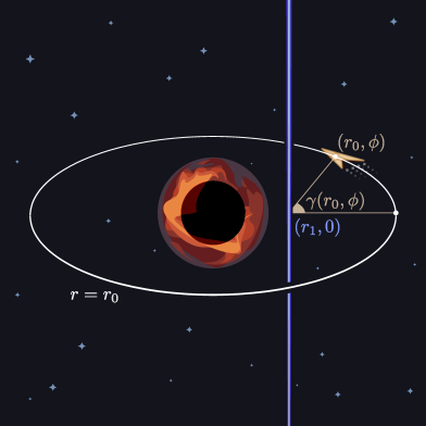
Figure 8: A spaceship is in circular orbit about a black hole adjacent to a chiral cosmic string. On board, a spinning top experiences an additional $\pi$ rotation of its spin per round trip, as compared to without the string.

Next, we compute the same spin holonomy but with the insertion of a symmetry operator $U_{\alpha}({\mathcal{S}})$. As depicted in Fig. 8, we take ${\mathcal{S}}$ to define the worldsheet of a chiral cosmic string spanning the azimuthal direction. Without loss of generality, let us take the string to intersect the plane $\theta=\pi/2$ at $(r,\phi)=(r_{1},0)$. The associated twisted Lorentz transformation is, for example,

$$\Omega=\exp\bigg{(}\hskip 1.00006pt{\frac{c}{2}\hskip 1.00006pt\gamma(r,\phi)}\hskip 0.50003pt\bigg{)}\qquad\resizebox{}{}{\scalebox{0.95}[0.95]{{\leavevmode\hbox{\set@color{\text{where}}}}}}\qquad e^{2\pi c}={\hbox to0.0pt{1\hss}\hskip 1.6pt\resizebox{}{}{\scalebox{1.1}[1.1]{{\leavevmode\hbox{\set@color{1}}}}}}\,,$$ (109)

which is simply an instance of Eq. (80) with $k=1$ winding. Here $\gamma(r,\phi)$ describes the “apparent” azimuthal angle measured from the string at $(r,\phi)=(r_{1},0)$, so concretely,

$$\tan\gamma(r,\phi)=\frac{r\sin\phi}{r\cos\phi{\,-\,}r_{1}}\,.$$ (110)

In principle, we can choose any generator for $c$ to demonstrate the transformation of the Wilson loop. For an explicit check, let us work out a simple case in which the multivalued transformation parameter $\Omega$ commutes with the spin connection component in Eq. (97). Namely, we take the Lorentz generator in Eq. (109) to be the self-dual generator in Eq. (108), so $c^{A}{}_{B}=(c_{+})^{A}{}_{B}$. By explicit calculation we find that the spin connection transforms according to

$$\begin{split}\omega^{A}{}_{B\phi}(r,\pi/2,\phi,t)=\frac{(c_{+}{\hskip 1.00006pt+\,}c_{-})^{A}{}_{B}}{2}\hskip 1.00006ptf(r)\,\,\,\mapsto\,\,\,\frac{(c_{+}{\hskip 1.00006pt+\,}c_{-})^{A}{}_{B}}{2}\hskip 1.00006ptf(r)+\frac{(c_{+})^{A}{}_{B}}{2}\hskip 1.00006pt\frac{\partial\gamma}{\partial\phi}(r,\phi)\,,\end{split}$$ (111)

where we have used that $(c_{+})^{A}{}_{B}$ commutes with $(c_{-})^{A}{}_{B}$. By construction the path ordering of this transformed spin connection is trivial and can be dropped. Finally, we find that the transformed spin holonomy is

$$\begin{split}{{W_{\text{{}vec}}({\mathcal{C}})}}\,\,\,\mapsto\,\,\,&\operatorname{tr}\exp\bigg{(}\hskip 1.00006pt{\frac{c_{+}{\hskip 1.00006pt+\,}c_{-}}{2}\hskip 1.00006pt2\pi f(r_{0})+\frac{c_{+}}{2}\hskip 1.00006pt2\pi n}\hskip 1.00006pt\bigg{)}\,,\\ &=2\cos n\pi+2\cos\Big{(}\hskip 1.00006pt{2\pi f(r_{0}){\,+\,}n\pi}\hskip 1.00006pt\Big{)}\,,\\ &=\Big{(}\hskip 1.00006pt{2{\,+\,}2\cos(\hskip 0.24994pt{2\pi f(r_{0})})}\Big{)}\cdot(-1)^{n}\,,\\ &={{W_{\text{{}vec}}({\mathcal{C}})}}\cdot(-1)^{n}\,,\end{split}$$ (112)

where $n$ is linking number measuring the number of times ${\mathcal{C}}$ winds about ${\mathcal{S}}$:

$$n\,=\frac{1}{2\pi}\int_{0}^{2\pi}\frac{\partial\gamma}{\partial\phi}(r,\phi)\hskip 1.00006ptd\phi\,=\hskip 1.00006pt\Bigg{\{}\begin{aligned} \,\,1&\quad\text{if}\quad r_{1}<r_{0}\,,\\ \,\,0&\quad\text{if}\quad r_{1}>r_{0}\,.\end{aligned}$$ (113)

Note how each term in Eq. (98) gets “twisted” to each term in Eq. (112), by the addition of $n\pi$ inside the argument of cosines. In conclusion, we find that the twisted local Lorentz transformation, which corresponds to an insertion of the operator $U_{\alpha}({\mathcal{S}})$, flips the sign of the spin holonomy when the contour ${\mathcal{C}}$ and the surface ${\mathcal{S}}$ are linked. This verifies the Ward identity for the one-form symmetry in a curved background.

More generally, it is possible to choose the twisted Lorentz transformation such that the twisted spin connection does not commute with itself at different points. In this case the path ordering in the spin holonomy is much more difficult to compute directly and so we resort to numerical methods. For example, let us consider an arbitrary self-dual generator parametrized by a unit three-vector $(n_{1},n_{2},n_{3})$:

$$c^{A}{}_{B}\,=\left({\begin{array}[]{cccc}\hphantom{\kern 9.49997pt}\mathclap{0}\hphantom{\kern 9.49997pt}&\hphantom{\kern 9.49997pt}\mathclap{n_{3}}\hphantom{\kern 9.49997pt}&\hphantom{\kern 9.49997pt}\mathclap{-n_{2}}\hphantom{\kern 9.49997pt}&\hphantom{\kern 9.49997pt}\mathclap{n_{1}}\hphantom{\kern 9.49997pt}\\ \hphantom{\kern 9.49997pt}\mathclap{-n_{3}}\hphantom{\kern 9.49997pt}&\hphantom{\kern 9.49997pt}\mathclap{0}\hphantom{\kern 9.49997pt}&\hphantom{\kern 9.49997pt}\mathclap{n_{1}}\hphantom{\kern 9.49997pt}&\hphantom{\kern 9.49997pt}\mathclap{n_{2}}\hphantom{\kern 9.49997pt}\\ \hphantom{\kern 9.49997pt}\mathclap{n_{2}}\hphantom{\kern 9.49997pt}&\hphantom{\kern 9.49997pt}\mathclap{-n_{1}}\hphantom{\kern 9.49997pt}&\hphantom{\kern 9.49997pt}\mathclap{0}\hphantom{\kern 9.49997pt}&\hphantom{\kern 9.49997pt}\mathclap{n_{3}}\hphantom{\kern 9.49997pt}\\ \hphantom{\kern 9.49997pt}\mathclap{-n_{1}}\hphantom{\kern 9.49997pt}&\hphantom{\kern 9.49997pt}\mathclap{-n_{2}}\hphantom{\kern 9.49997pt}&\hphantom{\kern 9.49997pt}\mathclap{-n_{3}}\hphantom{\kern 9.49997pt}&\hphantom{\kern 9.49997pt}\mathclap{0}\hphantom{\kern 9.49997pt}\end{array}}\right)=\,n_{1}\hskip 1.00006pt(t_{1}^{+})^{A}{}_{B}+n_{2}\hskip 1.00006pt(t_{2}^{+})^{A}{}_{B}+n_{3}\hskip 1.00006pt(t_{3}^{+})^{A}{}_{B}\,.$$ (118)

In this case the twisted spin connection is given by

$$\left({\begin{array}[]{cccc}\hphantom{\kern 5.24994pt}\mathclap{0}\hphantom{\kern 5.24994pt}&\hphantom{\kern 5.24994pt}\mathclap{0}\hphantom{\kern 5.24994pt}&\hphantom{\kern 5.24994pt}\mathclap{1}\hphantom{\kern 5.24994pt}&\hphantom{\kern 5.24994pt}\mathclap{0}\hphantom{\kern 5.24994pt}\\ \hphantom{\kern 5.24994pt}\mathclap{0}\hphantom{\kern 5.24994pt}&\hphantom{\kern 5.24994pt}\mathclap{0}\hphantom{\kern 5.24994pt}&\hphantom{\kern 5.24994pt}\mathclap{0}\hphantom{\kern 5.24994pt}&\hphantom{\kern 5.24994pt}\mathclap{1}\hphantom{\kern 5.24994pt}\\ \hphantom{\kern 5.24994pt}\mathclap{-1}\hphantom{\kern 5.24994pt}&\hphantom{\kern 5.24994pt}\mathclap{0}\hphantom{\kern 5.24994pt}&\hphantom{\kern 5.24994pt}\mathclap{0}\hphantom{\kern 5.24994pt}&\hphantom{\kern 5.24994pt}\mathclap{0}\hphantom{\kern 5.24994pt}\\ \hphantom{\kern 5.24994pt}\mathclap{0}\hphantom{\kern 5.24994pt}&\hphantom{\kern 5.24994pt}\mathclap{-1}\hphantom{\kern 5.24994pt}&\hphantom{\kern 5.24994pt}\mathclap{0}\hphantom{\kern 5.24994pt}&\hphantom{\kern 5.24994pt}\mathclap{0}\hphantom{\kern 5.24994pt}\end{array}}\right)\frac{f(r)}{2}-\left({\begin{aligned} {}&{}\Big{(}\hskip 1.00006pt{n_{2}n_{1}\hskip 1.00006pt\texttt{s}^{2}-n_{3}\hskip 1.00006pt\texttt{s}\texttt{c}}\hskip 1.00006pt\Big{)}\hskip 1.00006pt(t_{1}^{+})^{A}{}_{B}\\ {}+{}&{}\Big{(}\hskip 1.00006pt{\tfrac{1}{2}-(1{\hskip 1.00006pt-\,}{n_{2}}^{2})\hskip 1.00006pt\texttt{s}^{2}}\hskip 1.00006pt\Big{)}\hskip 1.00006pt(t_{2}^{+})^{A}{}_{B}\\ {}+{}&{}\Big{(}\hskip 1.00006pt{n_{2}n_{3}\hskip 1.00006pt\texttt{s}^{2}+n_{1}\hskip 1.00006pt\texttt{s}\texttt{c}}\hskip 1.00006pt\Big{)}\hskip 1.00006pt(t_{3}^{+})^{A}{}_{B}\end{aligned}}\right)f(r)+\frac{c^{A}{}_{B}}{2}\hskip 1.00006pt\frac{\partial\gamma}{\partial\phi}(r,\phi)\,,$$ (123)

where $\texttt{s}=\sin(\gamma(r,\phi)/2)$, $\texttt{c}=\cos(\gamma(r,\phi)/2)$. By evaluating the path-ordered exponential numerically, we can verify explicitly the final line of Eq. (112) for this more general case.

In the above examples we have always assumed that the holonomy contour and the chiral cosmic string are separated from the black hole horizon. Since the divergence of the line element in (90) at the horizon is a coordinate singularity, the loop and the string can actually be placed across or inside the horizon. It would be amusing to compute the holonomy in these more exotic configurations using coordinate systems in which the metric is regular on the horizon.

3.2 Canonical Formalism

Last but not least, let us now analyze the one-form symmetry of gravity from the point of view of the Hamiltonian formalism. The relevant framework is the nonchiral or real version of the Ashtekar ashtekar1986new formulation, as studied in Buffenoir:2004vx ; Alexandrov:2008fs ; Celada:2012ua ; Celada:2016bf .

3.2.1 Phase Space

In Eq. (52) we described the Lagrangian for tetradic Palatini gravity, expressed in terms of the Plebański two-form field. With all indices written out explicitly, this Lagrangian reads

$$\begin{split}\frac{1}{g^{2}}\hskip 1.00006pt\bigg{[}\hskip 1.00006pt{\frac{1}{2}\hskip 1.00006ptB_{a\mu\nu}\Big{(}{\partial_{\rho}\hskip 1.00006pt\omega^{a}{}_{\sigma}+{\textstyle\frac{1}{2}}\hskip 1.00006ptf^{a}{}_{bc}\hskip 1.00006pt\omega^{b}{}_{\rho}\hskip 1.00006pt\omega^{c}{}_{\sigma}}\Big{)}\hskip 1.00006pt\epsilon^{\mu\nu\rho\sigma}-\frac{\Lambda}{6}\hskip 1.00006ptB_{a\mu\nu}\hskip 0.50003pt{\star B}^{a}{}_{\rho\sigma}\hskip 1.00006pt\epsilon^{\mu\nu\rho\sigma}}\hskip 1.00006pt\bigg{]}\,.\end{split}$$ (124)

Carrying out the $3{\,+\,}1$ decomposition, we immediately find that the dynamical degrees of freedom coordinatizing the phase space are $\omega^{a}{}_{i}$ together with their canonical conjugates,

$$E^{i}{}_{a}=\frac{1}{2}\hskip 1.00006ptB_{ajk}\hskip 1.00006pt\epsilon^{ijk}\,.$$ (125)

Upon quantization, the canonical commutation relations are then

$$\begin{split}[\omega^{a}{}_{i}(x),\omega^{b}{}_{j}(x^{\prime})]&=0\,,\\ [E^{i}{}_{a}(x),\omega^{b}{}_{j}(x^{\prime})]&=g^{2}\,\delta^{i}{}_{j}\,\delta^{b}{}_{a}\,\delta^{(3)}(x{\,-\,}x^{\prime})\,,\\ [E^{i}{}_{a}(x),E^{j}{}_{b}(x^{\prime})]&=0\,,\end{split}$$ (126)

where $x,x^{\prime}\in{\mathcal{M}}_{3}$ are points in the spatial manifold. As expected, Eqs. (125) and (126) exactly mirror Eqs. (38) and (39) from gauge theory, which is indeed the entire point of the Ashtekar formulation ashtekar1986new ; Ashtekar:2020xll .

We restrict our focus to these canonical commutation relations, as they are the only crucial element for proving the one-form symmetry in Hamiltonian framework as we learned in Sec. 2.2. It is known that integrating out the nondynamical degrees of freedom eventually leads to a well-posed constrained Hamiltonian system equipped with several constraints Buffenoir:2004vx ; Alexandrov:2008fs ; Celada:2012ua ; Celada:2016bf , such as the Gauss constraints for local Lorentz transformations as well as the Hamiltonian and diffeomorphism constraints familiar from the ADM adm analysis.

3.2.2 Ward Identity

Following the logic of gauge theory, we now show how the one-form symmetry of gravity is implemented in the Hamiltonian formulation. Like before, we consider $W_{\rho}({\mathcal{C}})$ oriented in a spatial slice at $t{\,=\,}0$ and linked with $U_{\alpha}({\mathcal{S}})$. Again, we pancake ${\mathcal{S}}$ onto the spatial slice so that it becomes the disjoint union of two discs, defined by ${\mathcal{S}}={\mathcal{S}}_{+}{\hskip 1.00006pt\cup\hskip 1.00006pt}(-{\mathcal{S}}_{-})$. Here ${\mathcal{S}}_{+}$ and $-{\mathcal{S}}_{-}$ are two halves of a squashed sphere which straddle the spatial slice, as depicted in Fig. 5. These discs are eventually projected down to a surface ${\mathcal{S}}_{0}$ in the time slice $t{\,=\,}0$.

The symmetry operator factorizes into $U_{\alpha}({\mathcal{S}})=U_{\alpha}({\mathcal{S}}_{+})\hskip 1.00006ptU_{\alpha}(-{\mathcal{S}}_{-})$, so the symmetry transformation becomes the equal-time operator equation,

$$U_{\alpha}({\mathcal{S}}_{0})\,W_{\rho}({\mathcal{C}})\,U_{\alpha}\kern-3.00003pt\mathrlap{\leavevmode\hbox{\raise 1.1pt\hbox{\set@color\resizebox{}{}{{\leavevmode\hbox{\set@color{${}^{-1}$}}}}}}}\kern 9.49997pt({\mathcal{S}}_{0})\hskip 1.00006pt=\hskip 1.00006pt\rho(\alpha)^{\operatorname{int}_{3}({\mathcal{C}},{\mathcal{S}}_{0})}\,W_{\rho}({\mathcal{C}})\,,$$ (127)

where ${\mathcal{S}}_{0}$ and ${\mathcal{C}}$ all belong to the spatial three-dimensional manifold ${\mathcal{M}}_{3}$. Here $U_{\alpha}({\mathcal{S}}_{0})$ is the avatar of the symmetry operator in the Hamiltonian framework, taking a two-dimensional surface ${\mathcal{S}}_{0}$ with boundary as its support. Applying the $3{\,+\,}1$ decomposition described in the previous section, the symmetry operator becomes

$$U_{\alpha}({\mathcal{S}}_{0})=\exp\bigg{(}\hskip 1.00006pt{\frac{\pi}{g^{2}}\int_{{\mathcal{S}}_{0}}dx^{j}{\hskip 1.00006pt{\wedge}\,}dx^{k}\,\epsilon_{ijk}\hskip 1.00006ptE^{i}{}_{a}\hskip 1.00006pt\lambda^{a}}\bigg{)}\qquad\resizebox{}{}{\scalebox{0.95}[0.95]{{\leavevmode\hbox{\set@color{\text{where}}}}}}\qquad e^{2\pi\lambda}={\alpha}\,,$$ (128)

which exhibits the expected dependence on $E^{i}{}_{a}$ as the variable conjugate to the spin connection $\omega^{a}{}_{i}$. Using the canonical commutation relations in Eq. (126), the left-hand side of Eq. (127) can be evaluated as

$$\begin{split}U_{\alpha}({\mathcal{S}}_{0})\hskip 1.00006ptW_{\rho}({\mathcal{C}})\hskip 1.00006ptU_{\alpha}\kern-3.00003pt\mathrlap{\leavevmode\hbox{\raise 1.1pt\hbox{\set@color\resizebox{}{}{{\leavevmode\hbox{\set@color{${}^{-1}$}}}}}}}\kern 9.49997pt({\mathcal{S}}_{0})\hskip 1.00006pt&=\hskip 1.00006pt\operatorname{tr}_{\rho}\mathrm{P}\kern-1.00006pt\exp\bigg{(}\hskip 1.00006pt{\oint_{\mathcal{C}}\omega+2\pi\lambda\,\delta_{3}({\mathcal{S}}_{0})}\bigg{)}\hskip 1.00006pt=\hskip 1.00006pt\rho(\alpha)^{\operatorname{int}_{3}({\mathcal{C}},{\mathcal{S}}_{0})}\hskip 1.00006ptW_{\rho}(\mathcal{C})\,,\end{split}$$ (129)

thus establishing the Hamiltonian version of the Ward identity, introduced in Eq. (41) and reproduced in Eq. (127). Note the near isomorphism between Eqs. (128) and (129) for gravity and Eqs. (42) and (45) for gauge theory. Indeed, this parallel between Yang-Mills and gravity has been the central insight in our construction of the gravitational one-form symmetry. It also strongly aligns with the broader philosophy of the Ashtekar formulation, which is that Yang-Mills and gravity are formulated in essentially the same phase space.

We have taken as our starting point the definition of the spin holonomy in Eq. (58) and the symmetry operator in Eq. (66) and shown how these form the ingredients of a gravitational one-form symmetry. However, it is amusing that the reverse logic is actually possible. Starting from the spin holonomy, we can actually deduce the symmetry operator from first principles, as the line and charge operators are necessarily integrals of conjugate phase space variables. Specifically, this is required in order for their commutation relations to yield delta functions that eventually integrate to become field-independent linking numbers. Since $E^{i}{}_{a}$ is conjugate to the spin connection $\omega^{a}{}_{i}$, we see that Eq. (128) and its covariant counterpart were actually inevitable. Namely, this provides an alternative argument for the definition of the symmetry operator in Eq. (66).

3.3 Symmetry Breaking

As is well-known, global higher-form symmetries can be broken, either explicitly or spontaneously. In analogy with Yang-Mills theory, the one-form symmetry of gravity is explicitly broken in the presence of matter fields that transform nontrivially under the Lorentz group. For example, if the theory includes a local operator in the spin representation ${\rho}$, then it is possible to define a Lorentz invariant line holonomy $W_{{\rho}}({\mathcal{C}})$ for a contour ${\mathcal{C}}$ that is not closed, but rather terminates on this local operator. The spin holonomy is then “endable,” so it can be unlinked topologically from the symmetry operator $U_{\alpha}({\mathcal{S}})$, and the one-form symmetry is explicitly broken. The physical interpretation of this phenomenon is that the spin holonomy is screened by spinning particles.

$${\begin{array}[]{cc}\includegraphics[valign={c},scale={1.1}]{figs/screen-s.pdf}&\includegraphics[valign={c},scale={1.1}]{figs/screen-v.pdf}\end{array}}$$

Figure 9: Spinor holonomy is screened by fermions. Vector holonomy is screened by orbital angular momentum.

Interestingly, this implies that the gravitational one-form symmetry is explicitly broken by particles with spin. For example, if the Lorentz group is $G={\rm Spin}(4)$, then a holonomy in the spinor representation can only end on a local operator ${\cal O}_{\alpha}$ with a free spinor index. Hence, the corresponding holonomy is endable if there exist fermions in the spectrum. The case of $G={\rm SO}(4)$ is more subtle, however. A holonomy in the vector representation of the Lorentz group must end on an operator with a free Lorentz vector index, which can be any operator carrying orbital angular momentum dotted with a tetrad such as $e^{A}{}_{\mu}\nabla^{\mu}\mathcal{O}$. Consequently, the vector holonomy is analogous to the adjoint Wilson loop of gauge theory, which is automatically screened by dynamical gluons. See Fig. 9 for a depiction of this phenomenon.

The above logic has implications for the standard model of physics. Since fermions exist, we know that the Lorentz group is ${\rm SL}(2,\mathbb{C})$, which implies that there is a $\mathbb{Z}_{2}$ one-form gravitational symmetry under which spinor holonomies are charged. Presuming the lightest neutrino is not massless, this one-form symmetry is unbroken below that scale. This implies a new, albeit subtle, exact symmetry in the known laws of physics.

Notably, the explicit breaking of higher-form symmetry is strongly suggested by the so-called swampland conjectures. In particular, there is strong evidence that all global symmetries are necessarily broken at some scale in a consistent theory of quantum gravity Misner:1957mt ; Polchinski:2003bq ; Banks:2010zn ; Harlow:2018tng . A well-known avatar of this is the weak gravity conjecture Arkani-Hamed:2006emk ; Harlow:2022ich , which states that a $U(1)$ gauge theory must exhibit a state whose charge exceeds its mass in Planck units. The weak gravity conjecture quantitatively forbids the strict global symmetry limit of vanishing charge in a $U(1)$ gauge theory.

The swampland conjectures imply that any higher-form symmetry should be either gauged or explicitly broken. In the case of gauge theory coupled to gravity, the latter scenario requires the existence of a tower of charged states, as described by the so-called completeness conjectures Heidenreich:2021xpr . Applying the same logic to dynamical gravity, we expect that something similar applies to the gravitational one-form symmetry. One option is that this symmetry is gauged, for example as would occur if the Lorentz group is $\mathrm{Spin}(4)/{\mathbb{Z}_{2}}\times{\mathbb{Z}_{2}}$. Alternatively, if the Lorentz group is $\mathrm{Spin}(4)$, then the one-form symmetry is not gauged and must be explicitly broken, thus implying the existence of fermions in the spectrum.

Finally, let us speculate briefly on the possibility of phases in gravity. Taking inspiration from gauge theory, it is natural to wonder whether the expectation value of the spin holonomy is an order parameter for symmetry breaking. In the case of gauge theory, it is well-known that an area versus perimeter law scaling of the Wilson loop expectation value is a diagnostic of whether or not a theory is confining. However, the analogous construction in gravity is far murkier. In particular, as we noted earlier, the diffeomorphism invariance of dynamical gravity suggests that the contour of the spin holonomy—and any contour, actually—must be defined relationally with respect to some invariant boundary data. So to be an order parameter, the spin holonomy must presumably be computed for a contour that circumscribes the boundary.

Even ignoring these subtleties, the fact that the effective field theory description of gravity is intrinsically weakly coupled suggests that confinement is not in play. More generally it is very unclear whether a low-energy effective theory of gravity on a fixed background could even access different phases, or what that would even mean. One speculation is that this might have something to do with degenerate configurations of the metric and their corresponding domain walls Jacobson:1992xy ; Romano:1993bj ; Bengtsson:1997wr ; Volovik:1999vb . Another possibility is that a putative gravitational phase diagram might delineate various choices of compactification or of asymptotic behavior of the metric. Indeed, it is easy to see that the spin holonomy is highly sensitive to the cosmological constant. For these reasons, it would be interesting to explicitly compute the expectation value of the spin holonomy in various examples. A number of existing works have calculated the spin holonomy in various contexts Modanese:1993zh ; Modanese:1991nh ; Fredsted:2001rt ; Alawadhi:2021uie ; Jacobson:1992ya ; Donoghue:2016vck ; Brandhuber:2008tf .

4 Future Directions

In this paper, we have initiated an exploration of generalized symmetry in the context of dynamical gravity. Taking our cues from the one-form symmetries of Yang-Mills theory, we have considered gravity in the tetradic Palatini formalism, which is a gauge theory of the local Lorentz group. We have argued that the gravitational one-form symmetry is defined by the center of the Lorentz group. The object which is charged under this symmetry is the spin holonomy $W_{\rho}({\mathcal{C}})$. The one-form symmetry transformation is implemented by an operator $U_{\alpha}({\mathcal{S}})$, which has dual interpretations, both as a twisted Lorentz transformation but also as a chiral cosmic string defect carrying both electric and magnetic gravitational charge. The topological linking of the line and symmetry operators corresponds to the measurement of a quantized conical deficit angle by the spin holonomy. In the standard model, this implies the existence of a new symmetry below the mass of the lightest neutrino. The present work leaves numerous avenues for future exploration, which we now describe.

First and foremost are a number of very simple extensions of this work which should be relatively straightforward. These include the question of generalization to higher spacetime dimension, which offers a richer spectrum of one-form symmetry groups. For example, the center group is maximally $Z({\rm Spin}(4))=\mathbb{Z}_{2}{\hskip 1.00006pt\times\hskip 1.00006pt}\mathbb{Z}_{2}$ in four dimensions, but this grows to $Z({\rm Spin}(6))=\mathbb{Z}_{4}$ in six dimensions. Another concrete direction is the inclusion of gravitational higher-curvature corrections. These contributions will clearly preserve the one-form symmetry, whose corresponding symmetry operator will be equal to the surface integral of the canonical conjugate of the curvature in the effective field theory.

Secondly, while the present work has focused on gravitational one-form symmetry of electric type, it is natural to ask whether one can derive an analogous magnetic construction. For gauge theories, the electric and magnetic symmetry operators are straightforwardly related by the spacetime Hodge duality on the field strength Schafer-Nameki:2023jdn , which is computed with respect to a background volume form. For gravity, the analogous procedure necessarily introduces metric dependence, since the Levi-Civita permutation symbol is a density. This additional metric dependence implies that the putative magnetic symmetry operator is no longer the proper integral of a form. It is unclear whether this technical obstruction is insurmountable or merely peculiar. Meanwhile, recent work on cobordism classes in quantum gravity McNamara:2019rup appears to construct certain magnetic gravitational defects. Perhaps a direct link can be drawn between those results and the approach taken here.

A third topic of future study is higher-group symmetry, which describes a certain nonabelian structure built from the fusion of multiple higher-form symmetries Kapustin:2013uxa ; Benini:2018reh ; Cordova:2018cvg ; Cordova:2020tij . A well-studied example of this is axion-Yang-Mills theory, which exhibits a two-form symmetry for the axion, together with the one-form symmetry of the gauge theory Brennan:2020ehu . These symmetries fuse to yield a two-group structure, which in fact bounds the scale of axion strings from below by the lightest particle in the fundamental of color. Acquainted with this remarkable fact, it would be interesting to investigate if gravity can also exhibit a higher-group symmetry. It seems quite likely that a similar two-group symmetry will appear in gravity coupled to an axion, in which case we should expect that the axion string scale is bounded by the mass of the lightest fermion.

$${\begin{array}[]{ccc}\includegraphics[valign={c},width=130.08731pt]{figs/lattice4.pdf}&\xrightarrow[\displaystyle\text{ }]{\footnotesize\text{ \, twisted diffeo \, }}&\includegraphics[valign={c},width=130.08731pt]{figs/lattice6.pdf}\\ \leavevmode\hbox{$\vbox{\hbox{\resizebox{}{}{\scalebox{0.9}[0.9]{{\leavevmode\hbox{\set@color{ ``Empty Space'' }}}}}}}$}&&\leavevmode\hbox{$\vbox{\hbox{\resizebox{}{}{\scalebox{0.9}[0.9]{{\leavevmode\hbox{\set@color{ ``Cosmic String'' }}}}}}}$}\end{array}}$$

Figure 10: A diffeomorphism with a multivalued Jacobian creates a cosmic string from empty space, analogous to disinclinations in lattice systems.

Fourthly, while our approach of treating gravity as a “$BF\hskip 0.50003pt$”-type theory yields a simple route to the one-form symmetry, there is the question of how this framework is explicitly realized in other physically equivalent formulations of gravity krasnov2020formulations in the literature. For example, it is known that in the presence of a nonzero cosmological constant one can integrate out the tetrad altogether, yielding a theory of gravity described purely in terms of the spin connection Capovilla:1991kx ; Krasnov:2021zen . It would be interesting to understand the emergence of the gravitational one-form symmetry in this “pure connection” formalism given that all of our results were derived in the presence of a cosmological constant. Another open question is the fate of the one-form symmetry in gravitational formulations with subtly different field content, as referred to in a footnote in Sec. 3.3.

A fifth area of study concerns the question of what topological symmetry can teach us about classical gravitation. As a theory of spacetime geometry, gravity boasts a rich array of classical vacuum solutions, each showcasing distinctive singularity structures that are themselves a focal point of study penrose1965gravitational . In particular, it could be very illuminating to initiate a systematic analysis and classification of gravitational singularities from the perspective of topological operators and their algebra. For example, even in the absence of spin holonomy, the the one-form symmetry operator can link with “holes” in spacetime. It would be interesting to study whether there is physical information encoded in such a linking, for example regarding the singularity of a black hole. Moreover, it is conceivable that known spacetime singularities in the literature have an alternative interpretation as symmetry operators, like we discovered for the chiral cosmic string.

$${\begin{array}[]{ccc}\includegraphics[valign={c},width=156.10345pt]{figs/mbuild-0.pdf}&\xrightarrow[\displaystyle\text{ }]{\text{ \, twisted diffeo \, }}&\includegraphics[valign={c},width=156.10345pt]{figs/mbuild-1.pdf}\\ \leavevmode\hbox{$\vbox{\hbox{\resizebox{}{}{\scalebox{0.9}[0.9]{{\leavevmode\hbox{\set@color{ ``Empty Space'' }}}}}}}$}&&\leavevmode\hbox{$\vbox{\hbox{\resizebox{}{}{\scalebox{0.9}[0.9]{{\leavevmode\hbox{\set@color{ ``Misner String'' }}}}}}}$}\end{array}}$$

Figure 11: A multivalued diffeomorphism creates a Misner string from empty space, whose time monodromy is analogous to the Burgers vector of screw dislocations in lattice systems.

Last but not least, it would be interesting to see if the theoretical framework developed in this paper can be applied to lattice systems such as crystals with impurities chaikin1995principles ; Grozdanov:2018ewh ; Pace:2023kyi . Indeed, as described in Fiziev:1995te ; Kleinert:1996yi ; Kleinert:2008zzb , the physics of lattice systems has a formulation that is strikingly reminiscent of gravity. In this picture, lattice disinclinations are analogous to cosmic strings, as depicted in Fig. 10. Furthermore, the analog of “translation holonomy” is manifested by the Burgers vector, which measures the net drift in the “lattice frame” per round trip about a defect. Hence, as depicted in Fig. 11, we observe that lattice dislocations are analogous to the Misner string—a Dirac string of time monodromy flux endable on Taub-NUT charges Misner:1963flatter ; Misner:1965zz ; Bonnor:1969ala ; sackfield1971physical ; dowker1967gravitational ; cho1991magnetic ; Alfonsi:2020lub . These two types of lattice defects are described in terms of multivalued coordinate transformations Fiziev:1995te ; Kleinert:1996yi ; Kleinert:2008zzb , which are the diffeomorphism analogs of the twisted gauge transformations that played such a crucial role in our construction of a gravitational one-form symmetry. It would be interesting if this convergence between gravity and lattice systems could cross-pollinate new insights across these fields.

.

Acknowledgements. We are very much grateful to Clay Córdova, Kurt Hinterbichler, Ted Jacobson, Mrunmay Jagadale, Austin Joyce, Anton Kapustin, Jake McNamara, Julio Parra-Martinez, Matthew Reece, and Shu-Heng Shao for many insightful discussions and detailed comments on our draft. C.C., M.D., J.-H.K., V.N., and N.S. are supported by the Department of Energy (Grant No. DE-SC0011632) and by the Walter Burke Institute for Theoretical Physics. J.-H.K. is also supported in part by Ilju Academy and Culture Foundation. I.Z.R. is supported by the Department of Energy (Grant No. DE-FG02-04ER41338 and FG02-06ER41449).

Appendix A Notations and Conventions

Our results rely on numerous notational conventions and terminologies. For completeness, let us briefly summarize our nomenclature here.

Manifold and Index Conventions

Throughout our paper, the symbol ${\mathcal{M}}$ denotes the full four-dimensional manifold of spacetime. Within it resides zero-, one-, two-, and three-dimensional submanifolds, which we denote by ${\mathcal{P}}$, ${\mathcal{C}}$, ${\mathcal{S}}$, and ${\mathcal{V}}$, respectively. We often define ${\mathcal{S}}$ to be exact, so it is the boundary of a corresponding coboundary manifold ${\mathcal{V}}$ such that ${\mathcal{S}}=\partial{\mathcal{V}}$. On the other hand, we take ${\mathcal{C}}$ to be closed, so it has no boundary and thus $\partial{\mathcal{C}}=0$. In the Hamiltonian formalism, we perform a $3{\,+\,}1$ decomposition which generates quantities associated with a spatial three-dimensional submanifold ${\mathcal{M}}_{3}$, like the three-dimensional intersection number $\operatorname{int}_{3}$.

Spacetime indices are $\mu,\nu,\rho,\sigma,\ldots\in\{1,2,3,4\}$, while spatial indices are $i,j,k,l,\ldots\in\{1,2,3\}$. Adjoint indices of the Lorentz group are $a,b,c,d,\ldots\in\{1,2,3,4,5,6\}$ while vector indices are $A,B,C,D,\cdots\in\{1,2,3,4\}$. Undotted and dotted spinor indices are $\alpha,\beta,\gamma,\delta,\ldots\in\{0,1\}$ and ${\dot{\alpha}},{\dot{\beta}},{\dot{\gamma}},{\dot{\delta}},\ldots\in\{0,1\}$, respectively.

All epsilon tensors $\epsilon^{\mu\nu\rho\sigma}$ and $\epsilon_{\mu\nu\rho\sigma}$ are pure permutation symbols valued in $\{+1,-1,0\}$, sans dressing by metric-dependent determinant factors, so their indices are never partially raised or lowered. In particular, we employ the sign and normalization conventions,

$$\epsilon^{1234}=+1\,,\quad dx^{\mu}{\hskip 1.00006pt{\wedge}\,}dx^{\nu}{\hskip 1.00006pt{\wedge}\,}dx^{\rho}{\hskip 1.00006pt{\wedge}\,}dx^{\sigma}=\epsilon^{\mu\nu\rho\sigma}\hskip 1.00006ptd^{4}x\,,\quad\epsilon_{\mu\nu\rho\sigma}\hskip 1.00006pt\epsilon^{\mu\nu\rho\sigma}=+4!\,.$$ (130)

On the other hand, $\epsilon^{ABCD}$ and $\epsilon_{ABCD}$ have Lorentz vector indices which are raised and lowered by the flat Euclidean metric $\delta_{AB}=\operatorname{diag}(+1,+1,+1,+1)$.

Lorentz Algebra Conventions

Let us now summarize our conventions for the Lorentz Lie algebra. First of all, we employ an anti-Hermitian convention for Lie algebra generators $t_{a}$ so that $[t_{a},t_{b}]=f^{c}{}_{ab}\hskip 1.00006ptt_{c}$ without the imaginary unit. The adjoint and coadjoint actions on Lie algebra elements and their duals act as $(t_{a})^{i}{}_{j}\hskip 1.00006ptX^{a}\mapsto(\Omega^{-1})^{i}{}_{k}\hskip 1.00006pt(t_{a})^{k}{}_{l}\hskip 1.00006pt\Omega^{l}{}_{j}\hskip 1.00006ptX^{a}$ and $Y_{a}\hskip 1.00006pt(t^{a})^{i}{}_{j}\mapsto Y_{a}\hskip 1.00006pt(\Omega^{-1})^{i}{}_{k}\hskip 1.00006pt(t^{a})^{k}{}_{l}\hskip 1.00006pt\Omega^{l}{}_{j}$, respectively, so that $Y_{a}\hskip 1.00006ptX^{a}\propto Y_{a}\hskip 1.00006pt(t^{a}\hskip 0.24994ptt_{b})^{i}{}_{i}\hskip 1.00006ptX^{b}$ is invariant. In the main text, we have simply denoted these as $X^{a}\mapsto({\Omega}^{-1}{X}\hskip 1.00006pt{\Omega})^{a}$ and $Y_{a}\mapsto({\Omega}^{-1}{Y}\hskip 1.00006pt{\Omega})_{a}$.

The generators of the Lorentz Lie algebra $\mathfrak{so}(4)$ are six anti-symmetric matrices $(t_{a})^{AB}=(t_{a})^{[AB]}$, while those of the dual Lie algebra $\mathfrak{so}(4)^{*}$ are $(t^{a})_{\smash{AB}\vphantom{\beta}}=(t^{a})_{\smash{[AB]}\vphantom{\beta}}$. These are normalized according to

$$\delta^{a}{}_{b}={\textstyle\frac{1}{2}}\hskip 1.00006pt(t^{a})_{AB}\hskip 1.00006pt(t_{b})^{AB}\qquad\resizebox{}{}{\scalebox{0.95}[0.95]{{\leavevmode\hbox{\set@color{\text{and}}}}}}\qquad(t_{a})^{AB}\hskip 1.00006pt(t^{a})_{CD}=2\hskip 1.00006pt\delta^{[A}{}_{C}\hskip 1.00006pt\delta^{B]}{}_{D}\,.$$ (131)

Accordingly, raised and lowered adjoint indices are related to fundamental indices by

$$\begin{split}X^{AB}=(t_{a})^{AB}\hskip 1.00006ptX^{a}&\,,\quad X^{a}={\textstyle\frac{1}{2}}\hskip 1.00006pt(t^{a})_{AB}\hskip 1.00006ptX^{AB}\,,\\ Y_{AB}=Y_{a}\hskip 1.00006pt(t^{a})_{AB}&\,,\quad Y_{a}={\textstyle\frac{1}{2}}\hskip 1.00006ptY_{AB}\hskip 1.00006pt(t_{a})^{AB}\,.\end{split}$$ (132)

Note that the pairing between $\mathfrak{so}(4)$ and $\mathfrak{so}(4)^{*}$ is given by

$$Y_{a}\hskip 1.00006ptX^{a}={\textstyle\frac{1}{2}}\hskip 1.00006ptY_{AB}\hskip 1.00006ptX^{AB}\,.$$ (133)

Finally, the structure constants are

$$(t_{a})^{AB}\hskip 1.00006ptf^{a}{}_{bc}\hskip 1.00006ptX_{1}^{b}\hskip 1.00006ptX_{2}^{c}=X_{1}^{AC}\hskip 1.00006pt\delta_{CD}\hskip 1.00006ptX_{2}^{DB}-X_{2}^{AC}\hskip 1.00006pt\delta_{CD}\hskip 1.00006ptX_{1}^{DB}\,,$$ (134)

when expressed in the adjoint and fundamental representations.

Interestingly, two metrics can be endowed to the Lie algebra $\mathfrak{so}(4)$. Firstly, we have the usual positive-definite Killing form that universally exists in any dimensions:

$$\delta_{ab}={\textstyle\frac{1}{2}}\hskip 1.00006pt\delta_{AC}\hskip 1.00006pt\delta_{BD}\hskip 1.00006pt(t_{a})^{AB}\hskip 1.00006pt(t_{b})^{CD}\,,\quad\delta^{ab}={\textstyle\frac{1}{2}}\hskip 1.00006pt(t^{a})_{AB}\hskip 1.00006pt(t^{b})_{CD}\hskip 1.00006pt\delta^{AC}\hskip 1.00006pt\delta^{BD}\,,\quad\delta^{ac}\hskip 1.00006pt\delta_{cb}=\delta^{a}{}_{b}\,.$$ (135)

Indices are raised and lowered with this metric, which is consistent with the usual practice of raising and lowering fundamental indices with the flat Euclidean metric.

On the other hand, there is also a metric specific to four dimensions:

$$\textstyle{\hskip 0.50003pt\star\hskip 0.12497pt}_{ab}=\frac{1}{4}\hskip 1.00006pt\epsilon_{ABCD}\hskip 1.00006pt(t_{a})^{AB}\hskip 1.00006pt(t_{b})^{CD}\,,\quad{\hskip 0.50003pt\star\hskip 0.12497pt}^{ab}=\frac{1}{4}\hskip 1.00006pt(t^{a})_{AB}\hskip 1.00006pt(t^{b})_{CD}\hskip 1.00006pt\epsilon^{ABCD}\,,\quad{\hskip 0.50003pt\star\hskip 0.12497pt}^{ac}\hskip 0.50003pt{\hskip 0.50003pt\star\hskip 0.12497pt}_{cb}=\delta^{a}{}_{b}\,.$$ (136)

Evidently, this implements the Hodge dual. For instance,

$$\begin{split}({\hskip 0.50003pt\star\hskip 0.12497pt}_{ab}\hskip 1.00006ptX^{b})\hskip 1.00006pt(t^{a})_{AB}&={\textstyle\frac{1}{2}}\hskip 1.00006pt\epsilon_{ABCD}\hskip 1.00006ptX^{CD}={\star X}_{AB}\,,\\ (t_{a})^{AB}\hskip 1.00006pt({\hskip 0.50003pt\star\hskip 0.12497pt}^{ab}Y_{b})&={\textstyle\frac{1}{2}}\hskip 1.00006pt\epsilon^{ABCD}\hskip 1.00006ptY_{CD}={\star Y}^{AB}\,.\end{split}$$ (137)

Note that this metric naturally appears in the Palatini Lagrangian in Eq. (52). It has $(3,3)$ split signature, which connects to the decomposition $\mathfrak{so}(4)\cong\mathfrak{su}(2){\hskip 1.00006pt\oplus\,}\mathfrak{su}(2)$. Note also the identities

$${\hskip 0.50003pt\star\hskip 0.12497pt}^{ad}\delta_{dc}\hskip 1.00006pt{\hskip 0.50003pt\star\hskip 0.12497pt}^{ce}\delta_{eb}=\delta^{a}{}_{b}\,,\quad f^{a}{}_{bc}\hskip 1.00006pt{\hskip 0.50003pt\star\hskip 0.12497pt}^{be}\hskip 0.50003pt{\hskip 0.50003pt\star\hskip 0.12497pt}^{cf}=f^{a}{}_{bc}\hskip 1.00006pt\delta^{be}\hskip 0.50003pt\delta^{cf}\,,$$ (138)

which hold because the Hodge star squares to the identity in Euclidean signature.

Next, we discuss the spinor representations. In accordance with the isomorphism $\mathfrak{so}(4)\cong\mathfrak{su}(2){\hskip 1.00006pt\oplus\,}\mathfrak{su}(2)$, the six Lorentz generators split into two sets of $\mathfrak{su}(2)$ generators, which are symmetric $2{\,\times\,}2$ matrices normalized according to

$$\begin{split}\delta^{a}{}_{b}&=(\tilde{t}^{a})_{\smash{{\dot{\alpha}}{\dot{\beta}}}\vphantom{\beta}}\hskip 1.00006pt(\tilde{t}_{b})^{{\dot{\alpha}}{\dot{\beta}}}+(t^{a})_{\alpha\beta}\hskip 1.00006pt(t_{b})^{\alpha\beta}\,,\\ (\tilde{t}_{a})^{{\dot{\alpha}}{\dot{\beta}}}\hskip 1.00006pt(\tilde{t}^{a})_{\smash{{\dot{\gamma}}{\dot{\delta}}}\vphantom{\beta}}&=\delta^{({\dot{\alpha}}}{}_{\smash{{\dot{\gamma}}}\vphantom{\beta}}\hskip 1.00006pt\delta^{{\dot{\beta}})}{}_{\smash{{\dot{\delta}}}\vphantom{\beta}}\,,\quad(t_{a})^{\alpha\beta}\hskip 1.00006pt(t^{a})_{\smash{\gamma\delta}\vphantom{\beta}}=\delta_{\smash{\gamma}\vphantom{\beta}}{}^{(\alpha}\hskip 1.00006pt\delta_{\smash{\delta}\vphantom{\beta}}{}^{\beta)}\,.\end{split}$$ (139)

In accordance with the above, adjoint indices are unpacked to spinor indices as

$$\begin{split}\tilde{X}^{{\dot{\alpha}}{\dot{\beta}}}=(\tilde{t}_{a})^{{\dot{\alpha}}{\dot{\beta}}}X^{a}\,,\quad X^{a}=(\tilde{t}^{a})_{\smash{{\dot{\alpha}}{\dot{\beta}}}\vphantom{\beta}}\hskip 1.00006pt\tilde{X}^{{\dot{\alpha}}{\dot{\beta}}}&\,,\quad\tilde{Y}_{\smash{{\dot{\alpha}}{\dot{\beta}}}\vphantom{\beta}}=Y_{a}\hskip 1.00006pt(\tilde{t}^{a})_{\smash{{\dot{\alpha}}{\dot{\beta}}}\vphantom{\beta}}\,,\quad Y_{a}=\tilde{Y}_{\smash{{\dot{\alpha}}{\dot{\beta}}}\vphantom{\beta}}\hskip 1.00006pt(\tilde{t}_{a})^{{\dot{\alpha}}{\dot{\beta}}}\,,\\ X^{\alpha\beta}=(t_{a})^{\alpha\beta}X^{a}\,,\quad X^{a}=(t^{a})_{\smash{\alpha\beta}\vphantom{\beta}}\hskip 1.00006ptX^{\alpha\beta}&\,,\quad Y_{\smash{\alpha\beta}\vphantom{\beta}}=Y_{a}\hskip 1.00006pt(t^{a})_{\smash{\alpha\beta}\vphantom{\beta}}\,,\quad Y_{a}=Y_{\smash{\alpha\beta}\vphantom{\beta}}\hskip 1.00006pt(t_{a})^{\alpha\beta}\,.\end{split}$$ (140)

For example, it follows that

$$X^{a}=(\tilde{t}^{a})_{\smash{{\dot{\alpha}}{\dot{\beta}}}\vphantom{\beta}}\hskip 1.00006pt\tilde{X}^{{\dot{\alpha}}{\dot{\beta}}}+(t^{a})_{\smash{\alpha\beta}\vphantom{\beta}}\hskip 1.00006ptX^{\alpha\beta}\,,\quad Y_{a}\hskip 1.00006ptX^{a}=\tilde{Y}_{\smash{{\dot{\alpha}}{\dot{\beta}}}\vphantom{\beta}}\hskip 1.00006pt\tilde{X}^{{\dot{\alpha}}{\dot{\beta}}}+Y_{\alpha\beta}\hskip 1.00006ptX^{\alpha\beta}\,.$$ (141)

Also, the structure constants are given as

$$\begin{split}(t_{a})^{{\dot{\alpha}}{\dot{\beta}}}\hskip 1.00006ptf^{a}{}_{bc}\hskip 1.00006ptX_{1}^{b}\hskip 1.00006ptX_{2}^{c}&=(\tilde{X}_{1})^{{\dot{\alpha}}{\dot{\gamma}}}\hskip 1.00006pt{\tilde{\epsilon}}_{\smash{{\dot{\gamma}}{\dot{\delta}}}\vphantom{\beta}}\hskip 1.00006pt(\tilde{X}_{2})^{{\dot{\delta}}{\dot{\beta}}}-(\tilde{X}_{2})^{{\dot{\alpha}}{\dot{\gamma}}}\hskip 1.00006pt{\tilde{\epsilon}}_{\smash{{\dot{\gamma}}{\dot{\delta}}}\vphantom{\beta}}\hskip 1.00006pt(\tilde{X}_{1})^{{\dot{\delta}}{\dot{\beta}}}\,,\\ (t_{a})^{\alpha\beta}\hskip 1.00006ptf^{a}{}_{bc}\hskip 1.00006ptX_{1}^{b}\hskip 1.00006ptX_{2}^{c}&=(X_{1})^{\alpha\beta}\hskip 1.00006pt\epsilon_{\beta\delta}\hskip 1.00006pt(X_{2})^{\delta\gamma}-(X_{2})^{\alpha\beta}\hskip 1.00006pt\epsilon_{\beta\delta}\hskip 1.00006pt(X_{1})^{\delta\gamma}\,.\end{split}$$ (142)

The dotted generators describe self-dual (right-handed) rotations while the undotted generators describe anti-self-dual (left-handed) rotations:

$$\begin{split}{\hskip 0.50003pt\star\hskip 0.12497pt}_{ab}\hskip 1.00006pt(\tilde{t}^{b})_{\smash{{\dot{\alpha}}{\dot{\beta}}}\vphantom{\beta}}=+{\tilde{\epsilon}}_{\smash{{\dot{\alpha}}{\dot{\gamma}}}\vphantom{\beta}}\hskip 0.50003pt{\tilde{\epsilon}}_{\smash{{\dot{\beta}}{\dot{\delta}}}\vphantom{\beta}}\hskip 1.00006pt(\tilde{t}_{a})^{{\dot{\gamma}}{\dot{\delta}}}\,,\quad{\hskip 0.50003pt\star\hskip 0.12497pt}_{ab}\hskip 1.00006pt(t^{b})_{\smash{\alpha\beta}\vphantom{\beta}}=-\epsilon_{\alpha\gamma}\hskip 0.50003pt\epsilon_{\beta\delta}\hskip 1.00006pt(t_{a})^{\gamma\delta}\,.\end{split}$$ (143)

In fact, self-dual and anti-self-dual projectors arise as

$$\begin{split}(\tilde{t}^{a})_{\smash{{\dot{\alpha}}{\dot{\beta}}}\vphantom{\beta}}\hskip 1.00006pt(\tilde{t}^{b})_{\smash{{\dot{\gamma}}{\dot{\delta}}}\vphantom{\beta}}\hskip 1.00006pt{\tilde{\epsilon}}^{{\dot{\alpha}}{\dot{\gamma}}}\hskip 1.00006pt{\tilde{\epsilon}}^{{\dot{\beta}}{\dot{\delta}}}={\textstyle\frac{1}{2}}\hskip 1.00006pt(\hskip 0.24994pt{\delta^{ab}+{\hskip 0.50003pt\star\hskip 0.12497pt}^{ab}}\hskip 0.50003pt)\,,\quad(t^{a})_{\smash{\alpha\beta}\vphantom{\beta}}\hskip 1.00006pt(t^{b})_{\smash{\gamma\delta}\vphantom{\beta}}\hskip 1.00006pt\epsilon^{\alpha\gamma}\hskip 1.00006pt\epsilon^{\beta\delta}={\textstyle\frac{1}{2}}\hskip 1.00006pt(\hskip 0.24994pt{\delta^{ab}-{\hskip 0.50003pt\star\hskip 0.12497pt}^{ab}}\hskip 0.50003pt)\,.\end{split}$$ (144)

Having stated our conventions abstractly, let us be slightly more concrete and note that the self-dual and anti-self-dual generators are

$$(\tilde{t}^{AB})_{\smash{{\dot{\alpha}}{\dot{\beta}}}\vphantom{\beta}}={\textstyle\frac{1}{2}}\hskip 1.00006pt({\tilde{\epsilon}}\hskip 1.00006pt{\tilde{\sigma}}^{[A}\sigma^{B]})_{\smash{{\dot{\alpha}}{\dot{\beta}}}\vphantom{\beta}}\,,\quad(t^{AB})_{\alpha\beta}={\textstyle\frac{1}{2}}\hskip 1.00006pt(\sigma^{[A}{\tilde{\sigma}}^{B]}\epsilon)_{\alpha\beta}\,,$$ (145)

where an explicit representation of the Euclidean sigma matrices is given as

$$\begin{split}v_{A}\hskip 1.00006pt(\sigma^{A})_{\alpha{\dot{\alpha}}}=\bigg{(}{\begin{array}[]{cc}iv_{4}+v_{3}&v_{1}-iv_{2}\\ v_{1}+iv_{2}&iv_{4}-v_{3}\end{array}}\bigg{)}\,,\quad v_{A}\hskip 1.00006pt({\tilde{\sigma}}^{A})^{{\dot{\alpha}}\alpha}=\bigg{(}{\begin{array}[]{cc}iv_{4}-v_{3}&-v_{1}+iv_{2}\\ -v_{1}-iv_{2}&iv_{4}+v_{3}\end{array}}\bigg{)}\,,\end{split}$$ (146)

with the convention ${\tilde{\epsilon}}^{01}=\epsilon^{01}={\tilde{\epsilon}}_{10}=\epsilon_{10}=+1$ for the epsilon tensors.

Finally, we end with a demonstration of index conversions in the context of tetradic Palatini gravity. Let the spinor indices be raised and lowered as

$$\psi^{\alpha}=\epsilon^{\alpha\beta}\psi_{\beta}\,,\quad\psi_{\alpha}=\epsilon_{\alpha\beta}\hskip 1.00006pt\psi^{\beta}\,,\quad\tilde{\psi}^{\dot{\alpha}}={\tilde{\epsilon}}^{{\dot{\alpha}}{\dot{\beta}}}\tilde{\psi}_{\dot{\beta}}\,,\quad\tilde{\psi}_{\dot{\alpha}}={\tilde{\epsilon}}_{\smash{{\dot{\alpha}}{\dot{\beta}}}\vphantom{\beta}}\hskip 1.00006pt\tilde{\psi}^{\dot{\beta}}\,.$$ (147)

The spin connection splits into self-dual and anti-self-dual parts as

$$\omega^{a}=(\tilde{t}^{a})_{\smash{{\dot{\alpha}}{\dot{\beta}}}\vphantom{\beta}}\hskip 1.00006pt\tilde{\omega}^{{\dot{\alpha}}{\dot{\beta}}}+(t^{a})_{\smash{\alpha\beta}\vphantom{\beta}}\hskip 1.00006pt\omega^{\alpha\beta}\,.$$ (148)

The self-dual and anti-self-dual parts of the field strength are given by

$$\tilde{R}^{\dot{\alpha}}{}_{\dot{\beta}}=d\tilde{\omega}^{\dot{\alpha}}{}_{\dot{\beta}}-\tilde{\omega}^{\dot{\alpha}}{}_{\dot{\gamma}}{\hskip 1.00006pt{\wedge}\,}\tilde{\omega}^{\dot{\gamma}}{}_{\dot{\beta}}\,,\quad R_{\alpha}{}^{\beta}=d\omega_{\alpha}{}^{\beta}+\omega_{\alpha}{}^{\gamma}{\hskip 1.00006pt{\wedge}\,}\omega_{\gamma}{}^{\beta}\,.$$ (149)

Meanwhile, it is convenient to convert the vector index of the tetrad to spinor indices with a customary factor of $-1/2$, which originates from the $-2$ of $({\tilde{\sigma}}_{A})^{{\dot{\alpha}}\alpha}\hskip 1.00006pt(\sigma^{A})_{\smash{\beta{\dot{\beta}}}\vphantom{\beta}}=-2\hskip 1.00006pt\delta_{\smash{\beta}\vphantom{\beta}}{}^{\alpha}\hskip 1.00006pt\delta^{\dot{\alpha}}{}_{\smash{{\dot{\beta}}}\vphantom{\beta}}$:

$$e^{{\dot{\alpha}}\alpha}=-\frac{1}{2}\hskip 1.00006pt({\tilde{\sigma}}_{A})^{{\dot{\alpha}}\alpha}\hskip 1.00006pte^{A}\,.$$ (150)

Then the spinor components of the Plebański two-form defined in Eq. (51) are given by

$$\begin{split}\tilde{B}^{{\dot{\alpha}}{\dot{\beta}}}=\epsilon_{\smash{\alpha\beta}\vphantom{\beta}}\hskip 1.00006pte^{{\dot{\alpha}}\alpha}{\hskip 1.00006pt{\wedge}\,}e^{{\dot{\beta}}\beta}\,,\quad B^{\alpha\beta}=-{\tilde{\epsilon}}_{\smash{{\dot{\alpha}}{\dot{\beta}}}\vphantom{\beta}}\hskip 1.00006pte^{{\dot{\alpha}}\alpha}{\hskip 1.00006pt{\wedge}\,}e^{{\dot{\beta}}\beta}\,.\end{split}$$ (151)

In turn, the Lagrangian four-form in Eq. (52) boils down to

$$-\frac{1}{g^{2}}\hskip 1.00006pt\Big{(}\hskip 1.00006pt{e^{{\dot{\alpha}}\alpha}{\hskip 1.00006pt{\wedge}\,}e_{\smash{\alpha{\dot{\beta}}}\vphantom{\beta}}{\hskip 1.00006pt{\wedge}\,}\tilde{R}^{\dot{\beta}}{}_{\dot{\alpha}}+e_{\smash{\beta{\dot{\alpha}}}\vphantom{\beta}}\hskip 0.50003pt{\hskip 1.00006pt{\wedge}\,}e^{{\dot{\alpha}}\alpha}{\hskip 1.00006pt{\wedge}\,}R_{\alpha}{}^{\beta}}\hskip 1.00006pt\Big{)}+\frac{\Lambda}{3g^{2}}\hskip 1.00006pte_{\smash{\alpha{\dot{\alpha}}}\vphantom{\beta}}{\hskip 1.00006pt{\wedge}\,}e^{{\dot{\alpha}}\beta}{\hskip 1.00006pt{\wedge}\,}e_{\smash{\beta{\dot{\beta}}}\vphantom{\beta}}{\hskip 1.00006pt{\wedge}\,}e^{{\dot{\beta}}\alpha}\,.$$ (152)

The above expressions are consistent with the chiral symmetry operators in Eq. (68).

Appendix B Geometry of Linking

In this appendix, we expand on the technical details of the Dirac delta form and topological numbers in general spacetime dimension. Here we will indicate the dimensionality of each manifold with a subscript. All manifolds will be assumed to be orientable.

Definitions

Consider a $p$-dimensional submanifold ${\mathcal{N}}_{p}$ in a $d$-dimensional manifold $\mathcal{M}_{d}$. We define a differential form analog of Dirac’s delta distribution as

$$\int_{{\mathcal{N}}_{p}}\alpha^{(p)}\,\,\,=\,\,\int_{\mathcal{M}_{d}}\alpha^{(p)}\wedge\delta({\mathcal{N}}_{p})\,,$$ (153)

where $\alpha^{(p)}$ is an arbitrary smooth $p$-form in $\mathcal{M}_{d}$. Evidently, $\delta({\mathcal{N}}_{p})$ is a differential $(d{\,-\,}p)$-form distribution that peaks on the submanifold ${\mathcal{N}}_{p}$ while vanishing elsewhere.

More explicitly, suppose ${\mathcal{N}}_{p}$ is parameterized by coordinates $\sigma^{1},\sigma^{2},\cdots,\sigma^{p}$ as $x^{\mu}=X^{\mu}(\sigma)$, where $x^{\mu}$ denote coordinates of $\mathcal{M}_{d}$. Then $\delta({\mathcal{N}}_{p})$ is given by

$$\begin{split}\frac{1}{(d{\,-\,}p)!}\bigg{[}\,{\int d^{p}\sigma\,\,\delta^{(d)}(x{\,-\,}X(\sigma))\,\frac{\partial X^{\lambda_{1}}}{\partial\sigma^{1}}\cdots\frac{\partial X^{\lambda_{p}}}{\partial\sigma^{p}}}\,\bigg{]}\hskip 1.00006pt\epsilon_{\lambda_{1}\cdots\lambda_{p}\mu_{1}\cdots\mu_{d-p}}\hskip 1.00006ptdx^{\mu_{1}}{\hskip 1.00006pt{\wedge}\,}\cdots{\hskip 1.00006pt{\wedge}\,}dx^{\mu_{d-p}}\,,\end{split}$$ (154)

where $\delta^{(d)}(x{\,-\,}X(\sigma))$ is the ordinary Dirac delta function. This is higher-form generalization of Dirac delta function will be referred to as a “Dirac delta form.” The ordinary Dirac delta corresponds to $p=0$. It is also interesting to note that $\delta({\mathcal{N}}_{d})$ for a top-dimensional submanifold ${\mathcal{N}}_{d}$ is its characteristic function, e.g., $\delta({\mathcal{M}}_{d})=1$.

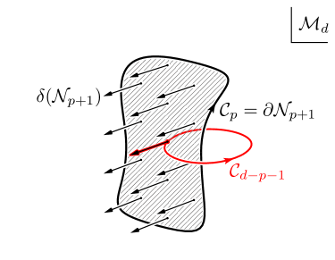
Figure 12: Linking between two submanifolds in $d$ dimensions.

In terms of Dirac delta forms, the intersection number between two orientable submanifolds ${\mathcal{N}}_{p}$ and ${\mathcal{N}}_{d-p}$ in ${\mathcal{M}}_{d}$ can be defined in a coordinate-free fashion:

$$\operatorname{int}({\mathcal{N}}_{p},{\mathcal{N}}_{d-p})\,=\int_{{\mathcal{M}}_{d}}\delta({\mathcal{N}}_{p}){\hskip 1.00006pt{\wedge}\,}\delta({\mathcal{N}}_{d-p})\,.$$ (155)

Note that the integrand $\delta({\mathcal{N}}_{p}){\hskip 1.00006pt{\wedge}\,}\delta({\mathcal{N}}_{d-p})$ is a top form that localizes at the intersection points. In fact, it could be argued that $\delta({\mathcal{N}}_{p}){\hskip 1.00006pt{\wedge}\,}\delta({\mathcal{N}}_{d-p})=\delta({\mathcal{N}}_{p}{\,\cap\,}{\mathcal{N}}_{d-p})$. It is instructive to check if Eq. (155) defines the intersection number in an expected way with specific values of $p$ and $d$, such as $p=0$, or $d=3$. Also, it is easy to see that

$$\operatorname{int}({\mathcal{N}}_{p},{\mathcal{N}}_{d-p})=(-1)^{p(d-p)}\,\operatorname{int}({\mathcal{N}}_{d-p},{\mathcal{N}}_{p})\,.$$ (156)

Given Eq. (155), we can easily define the linking number between two closed orientable submanifolds ${\mathcal{C}}_{p}$ and ${\mathcal{C}}_{d-p-1}$ provided that one of them is exact. Without loss of generality, suppose $\mathcal{C}_{p}=\partial{\mathcal{N}}_{p+1}$. Then we define

$$\operatorname{link}_{*}(\partial{\mathcal{N}}_{p+1},{\mathcal{C}}_{d-p-1})\,=\,\operatorname{int}({\mathcal{N}}_{p+1},{\mathcal{C}}_{d-p-1})\,=\int_{{\mathcal{C}}_{d-p-1}}\delta({\mathcal{N}}_{p+1})\,,$$ (157)

which counts how many times ${\mathcal{C}}_{d-p}$ penetrates the coboundary ${\mathcal{N}}_{p+1}$ as depicted in Fig. 12.

Note that the above definition necessarily puts the two arguments of $\operatorname{link}_{*}$ in an unequal footing: the first argument must be exact. However, as practiced in the main text, it can be convenient to use a more handy notation for the linking number such that the exact argument can be placed in any slot. With hindsight, we define such a notation “$\operatorname{link}$” to satisfy the following relations:

$$\begin{split}\operatorname{link}(\partial{\mathcal{N}}_{d-p},{\mathcal{C}}_{p})&=\operatorname{link}_{*}(\partial{\mathcal{N}}_{d-p},{\mathcal{C}}_{p})\,,\\ \operatorname{link}({\mathcal{C}}_{d-p-1},{\mathcal{C}}_{p})&=(-1)^{dp+1}\hskip 1.00006pt\operatorname{link}({\mathcal{C}}_{p},{\mathcal{C}}_{d-p-1})\,.\end{split}$$ (158)

The first equation states that $\operatorname{link}$ and $\operatorname{link}_{*}$ give the same number when the first argument is exact. The second equation allows the arguments of $\operatorname{link}$ to be freely rearranged, given the implicit assumption that one of the arguments is exact. The factor $(-1)^{dp+1}$ is necessitated from consistency with Eq. (161). Note also that the following holds:

$$\operatorname{link}({\mathcal{C}}_{d-p-1},\partial{\mathcal{N}}_{p+1}) =(-1)^{d-p}\hskip 1.00006pt\operatorname{int}({\mathcal{C}}_{d-p-1},{\mathcal{N}}_{p+1})\,.$$ (159)

Identities

Using either the coordinate-free/axiomatic definition of the Dirac delta form in Eq. (153) or the explicit definition in Eq. (154), one can derive various identities of Dirac delta forms and also intersection and linking numbers. Some simple ones are

$$d\hskip 1.00006pt\delta({\mathcal{N}}_{p}) =(-1)^{p}\,\delta(\partial{\mathcal{N}}_{p})\,,$$ (160)

$$\operatorname{link}(\partial{\mathcal{N}}_{p+1},\partial{\mathcal{N}}_{d-p}) =(-1)^{dp+1}\hskip 1.00006pt\operatorname{link}(\partial{\mathcal{N}}_{d-p},\partial{\mathcal{N}}_{p+1})\,.$$ (161)

The first identity encodes Stokes theorem, while the second identity describes a duality in the linking number computation.

A few more identities are found in the context of Hamiltonian formalism. Suppose the spacetime is a product manifold ${\mathcal{M}}_{d}={\mathcal{X}}_{d-1}{\hskip 1.00006pt\times\,}\mathbb{R}$ with coordinates $x^{\mu}=(x^{i},t)$, where the last coordinate $x^{\mu=d}{\,=\,}t$ labels hypersurfaces foliating ${\mathcal{M}}_{d}$. Then we consider submanifolds ${\mathcal{K}}_{p}$ and ${\mathcal{Y}}_{d-p-1}$ of ${\mathcal{X}}_{d-1}$ that can possibly intersect, with the former being closed: $\partial{\mathcal{K}}_{p}=0$. The corresponding relevant objects in spacetime are ${\mathcal{C}}_{p}$ and ${\mathcal{N}}_{d-p}$, defined as the following. First, we consider an embedding of the closed submanifold ${\mathcal{K}}_{p}$ in ${\mathcal{M}}_{d}$:

$${\mathcal{C}}_{p}={\mathcal{K}}_{p}{\hskip 1.00006pt\times\hskip 1.00006pt}\{t_{0}\}\,.$$ (162)

Second, we consider a timelike $(d{\,-\,}p)$-dimensional submanifold ${\mathcal{N}}_{d-p}$ of ${\mathcal{M}}_{d}$ defined as the following, where $\mathcal{I}=[t_{-},t_{+}]$ is an interval in $\mathbb{R}$ such that $t_{-}<t_{0}<t_{+}$:

$$(-1)^{d-p}\hskip 1.00006pt{\mathcal{N}}_{d-p}={\mathcal{Y}}_{d-p-1}{\hskip 1.00006pt\times\hskip 1.00006pt}\mathcal{I}\,.$$ (163)

The customary orientation of ${\mathcal{N}}_{d-p}$ by a sign factor $(-1)^{d-p}$ stipulates that its boundary is given in the form

$$\partial{\mathcal{N}}_{d-p}\,=\,\Big{(}\hskip 0.50003pt{-{\mathcal{Y}}_{d-p-1}{\hskip 1.00006pt\times\hskip 1.00006pt}\{t_{+}\}}\hskip 0.50003pt\Big{)}{\hskip 1.00006pt\,\cup\,\hskip 1.00006pt}\Big{(}\,{{\mathcal{Y}}_{d-p-1}{\hskip 1.00006pt\times\hskip 1.00006pt}\{t_{-}\}}\hskip 0.50003pt\Big{)}{\hskip 1.00006pt\,\cup\,\hskip 1.00006pt}\hskip 1.00006pt\Gamma\,,$$ (164)

for a timelike submanifold $\Gamma$ in ${\mathcal{M}}_{d}$. Specifically, the consistency between Eqs. (163) and (164) can be established by considering the Stokes theorem relating ${\mathcal{N}}_{d-p}$ and $\partial{\mathcal{N}}_{d-p}$, where a factor of $(-1)^{d-p-1}$ arising from rearranging the order of the time differential $dt$ combines with the minus sign in Eq. (164) to give $(-1)^{d-p}$.

With these definitions, it eventually follows that

$$(-1)^{d-p}\hskip 1.00006pt\operatorname{link}(\partial{\mathcal{N}}_{d-p},{\mathcal{C}}_{p})\hskip 1.00006pt=\hskip 1.00006pt\operatorname{int}({\mathcal{Y}}_{d-p-1}{\hskip 1.00006pt\times\hskip 1.00006pt}\mathcal{I},{\mathcal{C}}_{p})\hskip 1.00006pt=\hskip 1.00006pt(-1)^{p}\hskip 1.00006pt\operatorname{int}_{d-1}({\mathcal{Y}}_{d-p-1},{\mathcal{K}}_{p})\,,$$ (165)

where $\operatorname{int}_{d-1}({\mathcal{Y}}_{d-p-1},{\mathcal{K}}_{p})$ is the intersection number between ${\mathcal{Y}}_{d-p-1}$ and ${\mathcal{K}}_{p}$ in ${\mathcal{X}}_{d-1}$:

$$\operatorname{int}_{d-1}({\mathcal{Y}}_{d-p-1},{\mathcal{K}}_{p})\,\,=\hskip 1.00006pt\int_{{\mathcal{X}}_{d-1}}\delta_{d-1}({\mathcal{Y}}_{d-p-1}){\hskip 1.00006pt{\wedge}\,}\delta_{d-1}({\mathcal{K}}_{p})\,.$$ (166)

To derive Eq. (165), one may work in component terms with Eq. (154). One will find that the factor of $(-1)^{p}$ arises from an index rearrangement,

$$\epsilon_{i_{1}\cdots i_{d-p-1}d\hskip 0.70004ptj_{1}\cdots j_{p}}=(-1)^{p}\hskip 1.00006pt\epsilon_{i_{1}\cdots i_{d-p-1}j_{1}\cdots j_{p}d}=(-1)^{p}\hskip 1.00006pt\epsilon_{i_{1}\cdots i_{d-p-1}j_{1}\cdots j_{p}}\,,$$ (167)

where we work with the convention such that $\epsilon_{12\cdots d}=+1$.

Example: Abelian p-Form Symmetry in d Dimensions

Having derived various sign factors, we can describe a universal sign convention for higher-form symmetries of general rank $p$ in Euclidean signature spacetimes of general $d$ dimensions. Let us take an abelian $BF$ theory as a prototypical model, whose action reads

$$S\,\,=\int_{{\mathcal{M}}_{d}}B^{(d-p-1)}{\hskip 1.00006pt{\wedge}\,}F^{(p+1)}+f(B^{(d-p-1)})\,,$$ (168)

where $F^{(p+1)}=dA^{(p)}$. Here the superscripts denote the ranks, while $f(B^{(d-p-1)})$ is a $d$-form functional of $B^{(d-p-1)}$.

First, let us describe the $p$-form symmetry in the covariant formalism. For simplicity, consider the Wilson loop for an exact support:

$$W_{q}(\partial{\mathcal{N}}_{p+1})=\exp\bigg{(}\hskip 0.50003pt{q\int_{{\mathcal{N}}_{p+1}}F^{(p+1)}}\bigg{)}\,.$$ (169)

We want this to be transformed as

$$\begin{split}W_{q}(\partial{\mathcal{N}}_{p+1})\hskip 1.00006pt\,\,\mapsto\,\,\,\exp\Big{(}\hskip 1.00006pt{q\varepsilon\hskip 1.00006pt\operatorname{int}({\mathcal{C}}_{d-p-1},{\mathcal{N}}_{p+1})}\hskip 0.50003pt\Big{)}\,W_{q}(\partial{\mathcal{N}}_{p+1})\,,\end{split}$$ (170)

when the symmetry operator is inserted along an exact submanifold ${\mathcal{C}}_{d-p-1}=\partial{\mathcal{N}}_{d-p}$. Clearly, this can be undone by a field redefinition that shifts the field strength as $F^{(p+1)}\mapsto F^{(p+1)}-\varepsilon\,\delta({\mathcal{C}}_{d-p-1})$, which, in turn, transforms the action in Eq. (168) as

$$\begin{split}-S\,\,\,\mapsto\,\,-S\,+\,\varepsilon\int_{{\mathcal{M}}_{d}}\kern-1.00006ptB^{(d-p-1)}{\hskip 1.00006pt{\wedge}\,}\delta({\mathcal{C}}_{d-p-1})\,,\end{split}$$ (171)

from which the symmetry operator is identified:

$$U_{\varepsilon}({\mathcal{C}}_{d-p-1})=\exp\bigg{(}\hskip 1.00006pt{\varepsilon\int_{{\mathcal{C}}_{d-p-1}}\kern-6.00006ptB^{(d-p-1)}}\hskip 1.00006pt\bigg{)}\,.$$ (172)

Namely, the symmetry operator is derived as the term that is generated from the action term in the path integral after a field transformation that pushes the symmetry charge back into the defect operator. Crucially, the $BF$ structure leverages between the both sides of the Ward identity, which reads

$$\big{\langle}\hskip 0.50003pt{U_{\varepsilon}({\mathcal{C}}_{d-p-1})\hskip 1.00006ptW_{q}(\partial{\mathcal{N}}_{p+1})}\hskip 0.50003pt\big{\rangle}=\exp\Big{(}\hskip 1.00006pt{q\varepsilon\hskip 1.00006pt\operatorname{int}({\mathcal{C}}_{d-p-1},{\mathcal{N}}_{p+1})}\hskip 0.50003pt\Big{)}\,\big{\langle}\hskip 0.50003pt{W_{q}(\partial{\mathcal{N}}_{p+1})}\hskip 0.50003pt\big{\rangle}\,.$$ (173)

Finally, denoting ${\mathcal{C}}_{p}=\partial{\mathcal{N}}_{p+1}$, we can state the Ward identity in terms of a linking number:

$$\big{\langle}\hskip 0.50003pt{U_{\varepsilon}({\mathcal{C}}_{d-p-1})\hskip 1.00006ptW_{q}({\mathcal{C}}_{p})}\hskip 0.50003pt\big{\rangle}=\exp\Big{(}\hskip 1.00006pt{(-1)^{d-p}\hskip 1.00006ptq\varepsilon\hskip 1.00006pt\operatorname{link}({\mathcal{C}}_{d-p-1},{\mathcal{C}}_{p})}\hskip 0.50003pt\Big{)}\,\big{\langle}\hskip 0.50003pt{W_{q}({\mathcal{C}}_{p})}\hskip 0.50003pt\big{\rangle}\,,$$ (174)

which follows through using Eq. (159) (or Eqs. (156), (157), and (161) with $\operatorname{link}_{*}$).

Note that the Ward identities in the main text are reproduced when one takes $d{\,=\,}4$ and $p{\,=\,}1$ and makes the following identifications:

$${\mathcal{C}}_{p}\,\leftrightarrow\,{\mathcal{C}}\,,\quad{\mathcal{C}}_{d-p-1}\,\leftrightarrow\,{\mathcal{S}}\,,\quad{\mathcal{N}}_{d-p}\,\leftrightarrow\,{\mathcal{V}}\,.$$ (175)

Next, we can also double check from the angle of Hamiltonian formalism. Eq. (164) as a convetion for pancaking the coboundary ${\mathcal{N}}_{d-p}$ of the symmetry operator down to a submanifold ${\mathcal{Y}}_{d-p-1}$ in ${\mathcal{X}}_{d-1}$ stipulates that the Ward identity in Eq. (174) boils down to a conjugation of the defect operator as

$$e^{-\varepsilon Q({\mathcal{Y}}_{d-p-1})}\,W_{q}({\mathcal{K}}_{p})\,e^{\varepsilon Q({\mathcal{Y}}_{d-p-1})}=\exp\Big{(}\hskip 1.00006pt{(-1)^{p}\hskip 1.00006ptq\varepsilon\hskip 1.00006pt\operatorname{int}_{d-1}({\mathcal{Y}}_{d-p-1},{\mathcal{K}}_{p})}\hskip 0.50003pt\Big{)}\,W_{q}({\mathcal{C}}_{p})\,,$$ (176)

provided that the charge operator is defined as

$$Q({\mathcal{Y}}_{d-p-1})=\int_{{\mathcal{Y}}_{d-p-1}}\kern-6.00006ptB^{(d-p-1)}$$ (177)

as an object that lives in the $d{\,-\,}1$ dimensions. Note that the identity in Eq. (165) has been used to deduce Eq. (176) from Eq. (174). It is straightforward to verify Eq. (176) from the canonical commutation relations:

$$\begin{split}[A_{i_{1}\cdots i_{p}},B_{k_{1}\cdots k_{d-p-1}}]\,\epsilon^{k_{1}\cdots k_{d-p-1}j_{1}\cdots j_{p}}\hskip 1.00006pt&=\hskip 1.00006pt(d{\,-\,}p{\,-\,}1)!\hskip 1.00006ptp!\hskip 1.00006pt(-1)^{p}\,\delta^{j_{1}}{}_{\smash{[i_{1}}\vphantom{\beta}}{\cdots\,}\delta^{j_{p}}{}_{\smash{i_{p}]}\vphantom{\beta}}\,,\\ {{\implies}\quad}[A_{i_{1}\cdots i_{p}},Q({\mathcal{Y}}_{d-p-1})]\hskip 1.00006pt&=\hskip 1.00006pt(-1)^{p}\hskip 1.00006pt(\delta_{d-1}({\mathcal{Y}}_{d-p-1}))_{i_{1}\cdots i_{p}}\,,\end{split}$$ (178)

where the factor $(-1)^{p}$ precisely arises from the same index rearrangement as in Eq. (167), provided the conventions $\epsilon_{12\cdots d}=+1$ and $t=x^{d}$.

The above discussion corresponds to the calculation carried out in Secs. 2.2.2 and 3.2.2, so one can check consistency by taking $d{\,=\,}4$ and $p{\,=\,}1$. Yet, note that the spatial surface “${\mathcal{S}}_{0}$” there corresponds to ${\mathcal{Y}}_{d-p-1}$ here with a flip of orientation:

$${\mathcal{K}}_{p}\,\leftrightarrow\,{\mathcal{C}}\,,\quad{\mathcal{Y}}_{d-p-1}\,\leftrightarrow\,-{\mathcal{S}}_{0}\,.$$ (179)

This single flip is because the main text attempts to avoid any possible distractions from convention-dependent minus signs.

Proof of Equivalence between Eqs. (8) and (15)

Before ending, we should show that Eqs. (8) and (15), used in the main text, are equivalent statements. In $d$-dimensional spacetime, the claim reads

$$\begin{split}&\lim_{{\mathcal{P}}_{\pm}\to\,{\mathcal{P}}}\hskip 0.50003pt\Omega({\mathcal{P}}_{+})\hskip 1.00006pt\Omega^{-1}({\mathcal{P}}_{-})={\alpha}\in Z(G)\\ &\iff\quad\exists\,\lambda^{a}\qquad\resizebox{}{}{\scalebox{0.95}[0.95]{{\leavevmode\hbox{\set@color{\text{s.t.}}}}}}\qquad(\Omega^{-1}dd\Omega)^{a}=\lambda^{a}\hskip 1.00006pt\delta({\partial{\mathcal{V}}_{d-1}})\qquad\resizebox{}{}{\scalebox{0.95}[0.95]{{\leavevmode\hbox{\set@color{\text{and}}}}}}\qquad e^{2\pi\lambda}=\smash{{\alpha}^{(-1)^{d}}}\,,\end{split}$$ (180)

where ${\mathcal{P}}_{+}$ and ${\mathcal{P}}_{-}$ are points infinitesimally deviating from a point on ${\mathcal{V}}_{d-1}$ from above and below. The notion of above and below is well-defined, as ${\mathcal{V}}_{d-1}$ is oriented and codimension one. As shown below, the identities stated in Eqs. (156) and (161) play a role in the proof.

First of all, the fact that $\Omega$ as a multivalued function is everywhere smooth off the surface $\partial{\mathcal{V}}_{d-1}$ implies that $dd\Omega$ localizes on $\partial{\mathcal{V}}_{d-1}$ and vice versa, which is in turn equivalent to the existence of an algebra-valued zero-form $\lambda^{a}$ such that $(\Omega^{-1}dd\Omega)^{a}=2\pi\lambda^{a}\hskip 1.00006pt\delta({\partial{\mathcal{V}}_{d-1}})$.

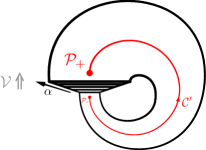
Figure 13: The center periodicity condition on the multivalued group parameter $\Omega$, in terms of the discontinuity $\lim_{{\mathcal{P}}_{\pm}\to\,{\mathcal{P}}}\hskip 0.50003pt(\hskip 0.12497pt\hskip 1.00006pt{\Omega({\mathcal{P}}_{+})\hskip 1.00006pt\Omega^{-1}({\mathcal{P}}_{-})}\hskip 0.50003pt)={\alpha}$ across a branch cut ${\mathcal{V}}$.

Thus, it remains to verify that the center periodicity condition on $\Omega$ is equivalent to $e^{2\pi\lambda}={\alpha}^{(-1)^{d}}$. It suffices to work with an exact one-dimensional loop ${\mathcal{C}}_{1}=\partial{\mathcal{N}}_{2}$ in the vicinity of $\partial{\mathcal{V}}_{d-1}$. Suppose $\operatorname{int}({\mathcal{V}}_{d-1},\partial{\mathcal{N}}_{2})=-1$. Then the periodicity condition implies

$$\begin{split}\lim_{{\mathcal{C}}^{\prime}_{1}\to\,{\mathcal{C}}_{1}}\hskip 0.50003pt\mathrm{P}\kern-1.00006pt\exp\bigg{(}\hskip 0.50003pt{\oint_{{\mathcal{C}}^{\prime}_{1}}\Omega^{-1}d\Omega}\bigg{)}=\lim_{{\mathcal{C}}^{\prime}_{1}\to\,{\mathcal{C}}_{1}}\hskip 0.50003pt\Omega^{-1}({\mathcal{P}}_{-})\hskip 1.00006pt\Omega({\mathcal{P}}_{+})=\alpha\,,\end{split}$$ (181)

where ${\mathcal{C}}^{\prime}_{1}$ is the infinitesimal opening of ${\mathcal{C}}_{1}$ described before. Meanwhile, the left-hand side can be computed as a surface-ordered integral, thanks to the nonabelian Stokes theorem:

$$\mathrm{P}\kern-1.00006pt\exp\bigg{(}\hskip 0.50003pt{\oint_{\partial{\mathcal{N}}_{2}}\Omega^{-1}d\Omega}\bigg{)}=\mathrm{P}\kern-1.00006pt\exp\bigg{(}\hskip 0.50003pt{\int_{{\mathcal{N}}_{2}}\Omega^{-1}dd\Omega}\bigg{)} =\exp\bigg{(}\hskip 0.50003pt{\int_{{\mathcal{M}}_{d}}\Omega^{-1}dd\Omega{\hskip 1.00006pt{\wedge}\,}\delta({\mathcal{N}}_{2})}\bigg{)}\,.$$ (182)

Note that the last equality has dropped the surface ordering because the integrand localizes at a single point. Plugging in $(\Omega^{-1}dd\Omega)^{a}=2\pi\lambda^{a}\hskip 1.00006pt\delta({\partial{\mathcal{V}}})$, the right-hand side boils down to $\exp\,(2\pi\lambda\hskip 1.00006pt\operatorname{int}(\partial{\mathcal{V}}_{d-1},{\mathcal{N}}_{2}))$, which equals $\exp\,((-1)^{d}\hskip 1.00006pt2\pi\lambda)$ given $\operatorname{int}({\mathcal{V}}_{d-1},\partial{\mathcal{N}}_{2})=-1$ by Eqs. (156) and (161). Therefore, demanding that the outcomes of Eqs. (181) and (182) are the same, we find $\alpha=\exp\,((-1)^{d}\hskip 1.00006pt2\pi\lambda)$, i.e., $e^{2\pi\lambda}={\alpha}^{(-1)^{d}}$. Lastly, recalling the fact that ${\alpha}{\,\in\,}Z(G)$, it can be seen that supposing generic curves with arbitrary linking numbers does not impose a further condition on $\lambda^{a}$. This concludes the proof.

To make it certain that all the signs have worked properly, it is instructive to double check by considering the abelian version of the statement:

$$\lim_{{\mathcal{P}}_{\pm}\to\,{\mathcal{P}}}\hskip 0.50003pt\chi({\mathcal{P}}_{+}){\,-\,}\chi({\mathcal{P}}_{-})=(-1)^{d}\hskip 1.00006pt2\pi\lambda\quad\iff\quad dd\chi=2\pi\lambda\,\delta({\partial{\mathcal{V}}_{d-1}})\,.$$ (183)

Here $\lambda$ is a constant. The periodicity condition in the left-hand side is equivalent to

$$d\chi+(-1)^{d}\hskip 1.00006pt2\pi\lambda\,\delta({\mathcal{V}}_{d-1})=df\,,$$ (184)

for some single-valued zero-form $f$; i.e., $d\chi$ is “gauge equivalent” to $(-1)^{d-1}\hskip 1.00006pt2\pi\lambda\,\delta({\mathcal{V}}_{d-1})$. Thus it follows that $dd\chi=(-1)^{d-1}\hskip 1.00006pt2\pi\lambda\,d\hskip 1.00006pt\delta({\mathcal{V}}_{d-1})$, which equals $2\pi\lambda\,\delta(\partial{\mathcal{V}}_{d-1})$ by Eq. (160).

Note that the points ${\mathcal{P}}_{+}$ and ${\mathcal{P}}_{-}$ in Fig. 2 are correctly deviating from above and below as stated in Eq. (LABEL:eq:claim) ($-\operatorname{link}({\mathcal{C}},{\mathcal{S}})=\operatorname{link}({\mathcal{S}},{\mathcal{C}})=\operatorname{int}({\mathcal{V}},{\mathcal{C}})=-1$), but the three-dimensional visualization seemingly appears the opposite due to the relative orientation with the hidden fourth dimension.

References

- (1) M. G. Alford and J. March-Russell, “Discrete gauge theories,” Int. J. Mod. Phys. B 5 (1991) 2641–2674.
- (2) M. G. Alford and J. March-Russell, “New order parameters for non-Abelian gauge theories,” Nucl. Phys. B 369 (1992) 276–298.
- (3) M. G. Alford, K.-M. Lee, J. March-Russell, and J. Preskill, “Quantum field theory of non-Abelian strings and vortices,” Nucl. Phys. B 384 (1992) 251–317, arXiv:hep-th/9112038.
- (4) M. Bucher, K.-M. Lee, and J. Preskill, “On detecting discrete Cheshire charge,” Nucl. Phys. B 386 (1992) 27–42, arXiv:hep-th/9112040.
- (5) T. Pantev and E. Sharpe, “Notes on gauging noneffective group actions,” arXiv:hep-th/0502027.
- (6) T. Pantev and E. Sharpe, “String compactifications on Calabi-Yau stacks,” Nucl. Phys. B 733 (2006) 233–296, arXiv:hep-th/0502044.
- (7) T. Pantev and E. Sharpe, “GLSM’s for Gerbes (and other toric stacks),” Adv. Theor. Math. Phys. 10 no. 1, (2006) 77–121, arXiv:hep-th/0502053.
- (8) S. Hellerman, A. Henriques, T. Pantev, E. Sharpe, and M. Ando, “Cluster decomposition, T-duality, and gerby CFT’s,” Adv. Theor. Math. Phys. 11 no. 5, (2007) 751–818, arXiv:hep-th/0606034.
- (9) Z. Nussinov and G. Ortiz, “A symmetry principle for topological quantum order,” Annals Phys. 324 (2009) 977–1057, arXiv:cond-mat/0702377.
- (10) O. Aharony, N. Seiberg, and Y. Tachikawa, “Reading between the lines of four-dimensional gauge theories,” JHEP 08 (2013) 115, arXiv:1305.0318 [hep-th].
- (11) D. Gaiotto, A. Kapustin, N. Seiberg, and B. Willett, “Generalized Global Symmetries,” JHEP 02 (2015) 172, arXiv:1412.5148 [hep-th].
- (12) N. Iqbal and J. McGreevy, “Mean string field theory: Landau-Ginzburg theory for 1-form symmetries,” SciPost Phys. 13 (2022) 114, arXiv:2106.12610 [hep-th].
- (13) X.-G. Wen, “Emergent anomalous higher symmetries from topological order and from dynamical electromagnetic field in condensed matter systems,” Phys. Rev. B 99 no. 20, (2019) 205139, arXiv:1812.02517 [cond-mat.str-el].
- (14) M. A. Levin and X.-G. Wen, “String net condensation: A Physical mechanism for topological phases,” Phys. Rev. B 71 (2005) 045110, arXiv:cond-mat/0404617.
- (15) M. A. Levin and X.-G. Wen, “Colloquium: Photons and electrons as emergent phenomena,” Rev. Mod. Phys. 77 (2005) 871–879, arXiv:cond-mat/0407140.
- (16) M. B. Hastings and X.-G. Wen, “Quasi-adiabatic continuation of quantum states: The Stability of topological ground state degeneracy and emergent gauge invariance,” Phys. Rev. B 72 (2005) 045141, arXiv:cond-mat/0503554.
- (17) H. Shimizu and K. Yonekura, “Anomaly constraints on deconfinement and chiral phase transition,” Phys. Rev. D 97 no. 10, (2018) 105011, arXiv:1706.06104 [hep-th].
- (18) Y. Choi, H. T. Lam, and S.-H. Shao, “Noninvertible Global Symmetries in the Standard Model,” Phys. Rev. Lett. 129 no. 16, (2022) 161601, arXiv:2205.05086 [hep-th].
- (19) C. Córdova and K. Ohmori, “Noninvertible Chiral Symmetry and Exponential Hierarchies,” Phys. Rev. X 13 no. 1, (2023) 011034, arXiv:2205.06243 [hep-th].
- (20) D. Gaiotto, A. Kapustin, Z. Komargodski, and N. Seiberg, “Theta, Time Reversal, and Temperature,” JHEP 05 (2017) 091, arXiv:1703.00501 [hep-th].
- (21) Z. Wan, J. Wang, and Y. Zheng, “New higher anomalies, SU(N) Yang–Mills gauge theory and sigma model,” Annals Phys. 414 (2020) 168074, arXiv:1812.11968 [hep-th].
- (22) L. V. Delacrétaz, D. M. Hofman, and G. Mathys, “Superfluids as Higher-form Anomalies,” SciPost Phys. 8 (2020) 047, arXiv:1908.06977 [hep-th].
- (23) P.-S. Hsin, H. T. Lam, and N. Seiberg, “Comments on One-Form Global Symmetries and Their Gauging in 3d and 4d,” SciPost Phys. 6 no. 3, (2019) 039, arXiv:1812.04716 [hep-th].
- (24) Y. Tanizaki, Y. Kikuchi, T. Misumi, and N. Sakai, “Anomaly matching for the phase diagram of massless -QCD,” Phys. Rev. D 97 no. 5, (2018) 054012, arXiv:1711.10487 [hep-th].
- (25) C. Córdova and K. Ohmori, “Anomaly Obstructions to Symmetry Preserving Gapped Phases,” arXiv:1910.04962 [hep-th].
- (26) Z. Wan and J. Wang, “Adjoint QCD4, Deconfined Critical Phenomena, Symmetry-Enriched Topological Quantum Field Theory, and Higher Symmetry-Extension,” Phys. Rev. D 99 no. 6, (2019) 065013, arXiv:1812.11955 [hep-th].
- (27) C. Córdova, D. S. Freed, H. T. Lam, and N. Seiberg, “Anomalies in the Space of Coupling Constants and Their Dynamical Applications I,” SciPost Phys. 8 no. 1, (2020) 001, arXiv:1905.09315 [hep-th].
- (28) C. Córdova, D. S. Freed, H. T. Lam, and N. Seiberg, “Anomalies in the Space of Coupling Constants and Their Dynamical Applications II,” SciPost Phys. 8 no. 1, (2020) 002, arXiv:1905.13361 [hep-th].
- (29) D. G. Delmastro, J. Gomis, P.-S. Hsin, and Z. Komargodski, “Anomalies and symmetry fractionalization,” SciPost Phys. 15 no. 3, (2023) 079, arXiv:2206.15118 [hep-th].
- (30) A. Kovner and B. Rosenstein, “New look at QED in four-dimensions: The Photon as a Goldstone boson and the topological interpretation of electric charge,” Phys. Rev. D 49 (1994) 5571–5581, arXiv:hep-th/9210154.
- (31) D. M. Hofman and N. Iqbal, “Goldstone modes and photonization for higher form symmetries,” SciPost Phys. 6 no. 1, (2019) 006, arXiv:1802.09512 [hep-th].
- (32) E. Lake, “Higher-form symmetries and spontaneous symmetry breaking,” arXiv:1802.07747 [hep-th].
- (33) N. Sogabe and N. Yamamoto, “Triangle Anomalies and Nonrelativistic Nambu-Goldstone Modes of Generalized Global Symmetries,” Phys. Rev. D 99 no. 12, (2019) 125003, arXiv:1903.02846 [hep-th].
- (34) I. Garcia Etxebarria and N. Iqbal, “A Goldstone theorem for continuous non-invertible symmetries,” JHEP 09 (2023) 145, arXiv:2211.09570 [hep-th].
- (35) C. Córdova and S. Koren, “Higher Flavor Symmetries in the Standard Model,” Annalen Phys. 535 no. 8, (2023) 2300031, arXiv:2212.13193 [hep-ph].
- (36) C. Córdova, S. Hong, S. Koren, and K. Ohmori, “Neutrino Masses from Generalized Symmetry Breaking,” arXiv:2211.07639 [hep-ph].
- (37) Y. Hidaka, M. Nitta, and R. Yokokura, “Higher-form symmetries and 3-group in axion electrodynamics,” Phys. Lett. B 808 (2020) 135672, arXiv:2006.12532 [hep-th].
- (38) Y. Hidaka, M. Nitta, and R. Yokokura, “Global 3-group symmetry and ’t Hooft anomalies in axion electrodynamics,” JHEP 01 (2021) 173, arXiv:2009.14368 [hep-th].
- (39) T. D. Brennan and C. Córdova, “Axions, higher-groups, and emergent symmetry,” JHEP 02 (2022) 145, arXiv:2011.09600 [hep-th].
- (40) Y. Choi, H. T. Lam, and S.-H. Shao, “Non-invertible Gauss law and axions,” JHEP 09 (2023) 067, arXiv:2212.04499 [hep-th].
- (41) R. Yokokura, “Non-invertible symmetries in axion electrodynamics,” arXiv:2212.05001 [hep-th].
- (42) T. D. Brennan, S. Hong, and L.-T. Wang, “Coupling a Cosmic String to a TQFT,” arXiv:2302.00777 [hep-ph].
- (43) Y. Choi, M. Forslund, H. T. Lam, and S.-H. Shao, “Quantization of Axion-Gauge Couplings and Non-Invertible Higher Symmetries,” arXiv:2309.03937 [hep-ph].
- (44) C. Córdova, S. Hong, and L.-T. Wang, “Axion Domain Walls, Small Instantons, and Non-Invertible Symmetry Breaking,” arXiv:2309.05636 [hep-ph].
- (45) M. Reece, “Axion-gauge coupling quantization with a twist,” JHEP 10 (2023) 116, arXiv:2309.03939 [hep-ph].
- (46) P. Agrawal and A. Platschorre, “The monodromic axion-photon coupling,” JHEP 01 (2024) 169, arXiv:2309.03934 [hep-th].
- (47) J. F. Donoghue, “Quantum General Relativity and Effective Field Theory,” arXiv:2211.09902 [hep-th].
- (48) C. P. Burgess, “Quantum gravity in everyday life: General relativity as an effective field theory,” Living Rev. Rel. 7 (2004) 5–56, arXiv:gr-qc/0311082.
- (49) J. McNamara and M. Reece, “Reflections on Parity Breaking,” arXiv:2212.00039 [hep-th].
- (50) J. McNamara and C. Vafa, “Cobordism Classes and the Swampland,” arXiv:1909.10355 [hep-th].
- (51) K. Hinterbichler, D. M. Hofman, A. Joyce, and G. Mathys, “Gravity as a gapless phase and biform symmetries,” JHEP 02 (2023) 151, arXiv:2205.12272 [hep-th].
- (52) V. Benedetti, H. Casini, and J. M. Magan, “Generalized symmetries of the graviton,” JHEP 05 (2022) 045, arXiv:2111.12089 [hep-th].
- (53) V. Benedetti, P. Bueno, and J. M. Magan, “Generalized Symmetries for Generalized Gravitons,” Phys. Rev. Lett. 131 no. 11, (2023) 111603, arXiv:2305.13361 [hep-th].
- (54) P. R. S. Gomes, “An introduction to higher-form symmetries,” SciPost Phys. Lect. Notes 74 (2023) 1, arXiv:2303.01817 [hep-th].
- (55) T. D. Brennan and S. Hong, “Introduction to Generalized Global Symmetries in QFT and Particle Physics,” arXiv:2306.00912 [hep-ph].
- (56) S. Schafer-Nameki, “ICTP Lectures on (Non-)Invertible Generalized Symmetries,” arXiv:2305.18296 [hep-th].
- (57) J. McGreevy, “Generalized Symmetries in Condensed Matter,” arXiv:2204.03045 [cond-mat.str-el].
- (58) C. Córdova, T. T. Dumitrescu, K. Intriligator, and S.-H. Shao, “Snowmass White Paper: Generalized Symmetries in Quantum Field Theory and Beyond,” in Snowmass 2021. 2021. arXiv:2205.09545 [hep-th].
- (59) E. Witten, “Wilson Loops, ’t Hooft Loops, and ’t Hooft’s Picture of Confinement,” in Quantum fields and strings: A course for mathematicians Vol.2, ch. 10, pp. 1255–1261. AMS, 1999.
- (60) L. Bhardwaj, L. E. Bottini, L. Fraser-Taliente, L. Gladden, D. S. W. Gould, A. Platschorre, and H. Tillim, “Lectures on generalized symmetries,” Phys. Rept. 1051 (2024) 1–87, arXiv:2307.07547 [hep-th].
- (61) S. Gukov and E. Witten, “Gauge Theory, Ramification, And The Geometric Langlands Program,” arXiv:hep-th/0612073.
- (62) D. Tong, “Gauge theory,” Lecture notes, DAMTP Cambridge 10 (2018) .
- (63) H. Reinhardt, “On ’t Hooft’s loop operator,” Phys. Lett. B 557 (2003) 317–323, arXiv:hep-th/0212264.
- (64) M. Engelhardt and H. Reinhardt, “Center projection vortices in continuum Yang-Mills theory,” Nucl. Phys. B 567 (2000) 249, arXiv:hep-th/9907139.
- (65) G. ’t Hooft, “On the Phase Transition Towards Permanent Quark Confinement,” Nucl. Phys. B 138 (1978) 1–25.
- (66) C. Córdova, K. Ohmori, and T. Rudelius, “Generalized symmetry breaking scales and weak gravity conjectures,” JHEP 11 (2022) 154, arXiv:2202.05866 [hep-th].
- (67) J. F. Plebański, “On the separation of Einsteinian substructures,” J. Math. Phys. 18 (1977) 2511–2520.
- (68) R. Capovilla, T. Jacobson, J. Dell, and L. J. Mason, “Self-dual 2-forms and gravity,” Class. Quant. Grav. 8 (1991) 41–57.
- (69) W. Donnelly and S. B. Giddings, “Observables, gravitational dressing, and obstructions to locality and subsystems,” Phys. Rev. D 94 no. 10, (2016) 104038, arXiv:1607.01025 [hep-th].
- (70) S. B. Giddings and J. Perkins, “Perturbative quantum evolution of the gravitational state and dressing in general backgrounds,” arXiv:2209.06836 [hep-th].
- (71) C. Rovelli and L. Smolin, “Discreteness of area and volume in quantum gravity,” Nucl. Phys. B 442 (1995) 593–622, arXiv:gr-qc/9411005. [Erratum: Nucl.Phys.B 456, 753–754 (1995)].
- (72) A. Ashtekar and J. Lewandowski, “Quantum theory of geometry. 1: Area operators,” Class. Quant. Grav. 14 (1997) A55–A82, arXiv:gr-qc/9602046.
- (73) J. D. Bekenstein, “Black holes and entropy,” Phys. Rev. D 7 (1973) 2333–2346.
- (74) S. W. Hawking, “Particle Creation by Black Holes,” Commun. Math. Phys. 43 (1975) 199–220. [Erratum: Commun.Math.Phys. 46, 206 (1976)].
- (75) Y. Cho, “Magnetic theory of gravitation,” in Primordial Nucleosynthesis and Evolution of Early Universe, pp. 203–211. Springer, 1991.
- (76) C. W. Misner, “The flatter regions of Newman, Unti and Tamburino’s generalized Schwarzschild space,” J. Math. Phys. 4 (1963) 924–938.
- (77) C. W. Misner, “Taub-NUT space as a counterexample to almost anything,” University of Maryland, Technical Report no. 529, (1965) .
- (78) W. B. Bonnor, “A new interpretation of the NUT metric in general relativity,” Math. Proc. Cambridge Phil. Soc. 66 no. 1, (1969) 145–151.
- (79) A. Sackfield, “Physical interpretation of NUT metric,” in Mathematical Proceedings of the Cambridge Philosophical Society, vol. 70, pp. 89–94, Cambridge University Press. 1971.
- (80) J. S. Dowker and J. A. Roche, “The Gravitational analogues of magnetic monopoles,” Proc. Phys. Soc. 92 (1967) 1–8.
- (81) A. H. Taub, “Empty space-times admitting a three parameter group of motions,” Annals Math. 53 (1951) 472–490.
- (82) E. Newman, L. Tamburino, and T. Unti, “Empty space generalization of the Schwarzschild metric,” J. Math. Phys. 4 (1963) 915.
- (83) L. Alfonsi, C. D. White, and S. Wikeley, “Topology and Wilson lines: global aspects of the double copy,” JHEP 07 (2020) 091, arXiv:2004.07181 [hep-th].
- (84) M. J. Duff, “Quantum Tree Graphs and the Schwarzschild Solution,” Phys. Rev. D 7 (1973) 2317–2326.
- (85) C. Cheung, J. Parra-Martinez, I. Z. Rothstein, N. Shah, and J. Wilson-Gerow, “Effective Field Theory for Extreme Mass Ratios,” arXiv:2308.14832 [hep-th].
- (86) G. Modanese, “Wilson loops in four-dimensional quantum gravity,” Phys. Rev. D 49 (1994) 6534–6542, arXiv:hep-th/9307148.
- (87) J. Fredsted, “Comment on Wilson loops in four-dimensional quantum gravity,” Phys. Rev. D 64 (2001) 088501.
- (88) A. Ashtekar, “New Variables for Classical and Quantum Gravity,” Phys. Rev. Lett. 57 (1986) 2244–2247.
- (89) E. Buffenoir, M. Henneaux, K. Noui, and P. Roche, “Hamiltonian analysis of Plebanski theory,” Class. Quant. Grav. 21 (2004) 5203–5220, arXiv:gr-qc/0404041.
- (90) S. Alexandrov and K. Krasnov, “Hamiltonian Analysis of non-chiral Plebanski Theory and its Generalizations,” Class. Quant. Grav. 26 (2009) 055005, arXiv:0809.4763 [gr-qc].
- (91) M. Celada and M. Montesinos, “Lorentz-covariant Hamiltonian analysis of BF gravity with the Immirzi parameter,” Class. Quant. Grav. 29 (2012) 205010, arXiv:1209.0396 [gr-qc].
- (92) M. Celada, D. González, and M. Montesinos, “ gravity,” Class. Quant. Grav. 33 no. 21, (2016) 213001, arXiv:1610.02020 [gr-qc].
- (93) A. Ashtekar and M. Varadarajan, “Gravitational Dynamics—A Novel Shift in the Hamiltonian Paradigm,” Universe 7 no. 1, (2021) 13, arXiv:2012.12094 [gr-qc].
- (94) R. L. Arnowitt, S. Deser, and C. W. Misner, “Dynamical Structure and Definition of Energy in General Relativity,” Phys. Rev. 116 (1959) 1322–1330.
- (95) H. Urbantke, “On integrability properties of SU(2) Yang–Mills fields. I. Infinitesimal part,” J. Math. Phys. 25 no. 7, (1984) 2321–2324.
- (96) C. W. Misner and J. A. Wheeler, “Classical physics as geometry: Gravitation, electromagnetism, unquantized charge, and mass as properties of curved empty space,” Annals Phys. 2 (1957) 525–603.
- (97) J. Polchinski, “Monopoles, duality, and string theory,” Int. J. Mod. Phys. A 19S1 (2004) 145–156, arXiv:hep-th/0304042.
- (98) T. Banks and N. Seiberg, “Symmetries and Strings in Field Theory and Gravity,” Phys. Rev. D 83 (2011) 084019, arXiv:1011.5120 [hep-th].
- (99) D. Harlow and H. Ooguri, “Symmetries in quantum field theory and quantum gravity,” Commun. Math. Phys. 383 no. 3, (2021) 1669–1804, arXiv:1810.05338 [hep-th].
- (100) N. Arkani-Hamed, L. Motl, A. Nicolis, and C. Vafa, “The String Landscape, Black Holes and Gravity as the Weakest Force,” JHEP 06 (2007) 060, arXiv:hep-th/0601001.
- (101) D. Harlow, B. Heidenreich, M. Reece, and T. Rudelius, “Weak gravity conjecture,” Rev. Mod. Phys. 95 no. 3, (2023) 035003, arXiv:2201.08380 [hep-th].
- (102) B. Heidenreich, J. McNamara, M. Montero, M. Reece, T. Rudelius, and I. Valenzuela, “Non-invertible global symmetries and completeness of the spectrum,” JHEP 09 (2021) 203, arXiv:2104.07036 [hep-th].
- (103) T. Jacobson and J. D. Romano, “Degenerate extensions of general relativity,” Class. Quant. Grav. 9 (1992) L119–L124, arXiv:gr-qc/9207005.
- (104) J. D. Romano, “On the constraint algebra of degenerate relativity,” Phys. Rev. D 48 (1993) 5676–5683, arXiv:gr-qc/9306034.
- (105) I. Bengtsson and T. Jacobson, “Degenerate metric phase boundaries,” Class. Quant. Grav. 14 no. 11, (1997) 3109–3121, arXiv:gr-qc/9706027. [Erratum: Class.Quant.Grav. 15, 3941–3942 (1998)].
- (106) G. E. Volovik, “Vierbein walls in condensed matter,” JETP Lett. 70 (1999) 711–716, arXiv:gr-qc/9911026.
- (107) G. Modanese, “Geodesic round trips by parallel transport in quantum gravity,” Phys. Rev. D 47 (1993) 502–509.
- (108) R. Alawadhi, D. S. Berman, C. D. White, and S. Wikeley, “The single copy of the gravitational holonomy,” JHEP 10 (2021) 229, arXiv:2107.01114 [hep-th].
- (109) T. Jacobson and J. D. Romano, “The Spin holonomy group in general relativity,” Commun. Math. Phys. 155 (1993) 261–276, arXiv:gr-qc/9207006.
- (110) J. F. Donoghue, “Is the spin connection confined or condensed?,” Phys. Rev. D 96 no. 4, (2017) 044003, arXiv:1609.03523 [hep-th].
- (111) A. Brandhuber, P. Heslop, A. Nasti, B. Spence, and G. Travaglini, “Four-point Amplitudes in N=8 Supergravity and Wilson Loops,” Nucl. Phys. B 807 (2009) 290–314, arXiv:0805.2763 [hep-th].
- (112) A. Kapustin and R. Thorngren, “Higher Symmetry and Gapped Phases of Gauge Theories,” Prog. Math. 324 (2017) 177–202, arXiv:1309.4721 [hep-th].
- (113) F. Benini, C. Córdova, and P.-S. Hsin, “On 2-Group Global Symmetries and their Anomalies,” JHEP 03 (2019) 118, arXiv:1803.09336 [hep-th].
- (114) C. Córdova, T. T. Dumitrescu, and K. Intriligator, “Exploring 2-Group Global Symmetries,” JHEP 02 (2019) 184, arXiv:1802.04790 [hep-th].
- (115) C. Córdova, T. T. Dumitrescu, and K. Intriligator, “2-Group Global Symmetries and Anomalies in Six-Dimensional Quantum Field Theories,” JHEP 04 (2021) 252, arXiv:2009.00138 [hep-th].
- (116) K. Krasnov, Formulations of general relativity: Gravity, spinors and differential forms. Cambridge University Press, 2020.
- (117) R. Capovilla, T. Jacobson, and J. Dell, “A pure spin connection formulation of gravity,” Class. Quant. Grav. 8 (1991) 59–73.
- (118) K. Krasnov and E. Mitsou, “Pure Lorentz spin connection theories and uniqueness of general relativity,” Class. Quant. Grav. 38 no. 20, (2021) 205009, arXiv:2106.05803 [gr-qc].
- (119) R. Penrose, “Gravitational collapse and space-time singularities,” Physical Review Letters 14 no. 3, (1965) 57.
- (120) P. M. Chaikin, T. C. Lubensky, and T. A. Witten, Principles of condensed matter physics, vol. 10. Cambridge university press Cambridge, 1995.
- (121) S. Grozdanov and N. Poovuttikul, “Generalized global symmetries in states with dynamical defects: The case of the transverse sound in field theory and holography,” Phys. Rev. D 97 no. 10, (2018) 106005, arXiv:1801.03199 [hep-th].
- (122) S. D. Pace, “Emergent generalized symmetries in ordered phases,” arXiv:2308.05730 [cond-mat.str-el].
- (123) P. Fiziev and H. Kleinert, “New action principle for classical particle trajectories in spaces with torsion,” EPL 35 (1996) 241–246, arXiv:hep-th/9503074.
- (124) H. Kleinert and A. Pelster, “Lagrange mechanics in spaces with curvature and torsion,” Gen. Rel. Grav. 31 (1999) 1439, arXiv:gr-qc/9605028.
- (125) H. Kleinert, Multivalued fields. In condensed matter, electromagnetism, and gravitation. World Scientific, 2008.