Graphical $n$-sample tests of correspondence of distributions

Abstract

Classical tests are available for the two-sample test of correspondence of distribution functions. From these, the Kolmogorov-Smirnov test provides also the graphical interpretation of the test results, in different forms. Here, we propose modifications of the Kolmogorov-Smirnov test with higher power. The proposed tests are based on the so-called global envelope test which allows for graphical interpretation, similarly as the Kolmogorov-Smirnov test. The tests are based on rank statistics and are suitable also for the comparison of $n$ samples, with $n\geq 2$. We compare the alternatives for the two-sample case through an extensive simulation study and discuss their interpretation. Finally, we apply the tests to real data. Specifically, we compare the height distributions between boys and girls at different ages, as well as sepal length distributions of different flower species using the proposed methodologies.

1 Introduction

In statistical theory, hypothesis testing has a central role. Often, statisticians need to address whether the distribution of a population follows a theoretical distribution. These types of tests are often referred to as goodness-of-fit tests in the literature. For instance, the Shapiro-Wilk test (Shaphiro and Wilk, 1965) is a goodness-of-fit test that tests for Gaussianity of the underlying population. However, the test lacks a graphical illustration of the test result. Alternatively, various graphical goodness-of-fit procedures (Kolmogorov, 1933; Warton, 2022; Aldor-Noiman et al., 2013) for testing the Gaussianity of the underlying population also provide graphical visualization of the test outcome.

Goodness-of-fit tests can be extended to investigate whether distributions of two populations are different, and if they are, how they differ. Statistical tests for comparing the distributions of two samples can be constructed by considering test statistics defined as deviations between the empirical cumulative distribution functions of the two samples. Classical examples of such tests are the two-sample Kolmogorov-Smirnov (KS) test (Kolmogorov, 1933), Cramér von Mises test (Cramér, 1928) and Anderson-Darling test (Anderson and Darling, 1954). Among these tests, only the KS test can provide a graphical interpretation of the test results, i.e., a graphical illustration showing the reason for rejecting the null hypothesis. On the other hand, the KS test has some disadvantages. First and foremost, it is an asymptotic test, and hence it requires ”large” sample sizes to be valid. Second, it is designed only for comparing two continuous distributions which limits its applicability. Third, it is more sensitive around the median of the two distributions and gives low statistical power when distributional differences lie in the tails (see e.g. Aldor-Noiman et al., 2013).

Statistical tests for the distribution comparison of two samples can be constructed using Monte Carlo methods. Such tests are non-parametric, based on data permutations and evaluation of a test statistic expressing a distributional contrast. For instance, the R (R Core Team, 2023) package twosamples (Dowd, 2023) implements permutation tests with contrasts defined as deviations between the empirical cumulative distribution functions (Dowd, 2020). Among others, permutation tests based on the Kolmogorov-Smirnov, Kuiper (Kuiper, 1960) and Wasserstein (Vaserstein, 1969) deviations are available. Permutation tests can also be constructed by considering deviation measures between the two probability density functions. A rigorous review of potential test statistics, i.e., deviation measures between two densities, is presented by (Cha, 2007), in which the measures are categorized into seven main families. The Minkowski $L_{p}$ family, the $L_{1}$ family, the intersection family, the inner product family, the fidelity family, the squared $L_{2}$ family, and the Shannon’s entropy family. Finally, distances combining ideas from measures from the aforementioned families are also possible. Implementations of the aforementioned distances are available in the R package philentropy (Hajk-Georg, 2018). However, similarly to the classical Cramér von Mises, Monte Carlo tests that are based on these other measures than the Kolmogorov-Smirnov measure do not provide any graphical interpretation of the test results and therefore are not considered in our analyses.

In this paper, we propose graphical tests for comparing the distributions of $n$ samples, with $n\geq 2$. The proposed tests are non-parametric, permutation tests based on the global envelope testing framework proposed by Myllymäki et al. (2017). Global envelope tests provide a multiple testing adjustment procedure for testing statistical hypotheses involving multivariate or functional test statistics. That is, given a $d$-dimensional discretization of a test statistic $T$ and a significance level $\alpha$, the multiple testing issue is solved by controlling the family-wise error rate. Further, the tests provide graphical interpretation in the form of a $100(1-\alpha)\%$ global envelope, i.e., a $100(1-\alpha)\%$ acceptance region under the null hypothesis of the equality of the distributions of $n$ samples. That is, the null hypothesis is rejected if and only if the empirical test statistic falls outside the acceptance region at any point of the discretization. Further, the graphical interpretation allows for investigating the reasons for rejecting the null hypothesis.

The tests are based on ranking the ”extremeness” of the empirical test statistic among simulations produced under the null hypothesis, using a ranking measure. Thus, a prerequisite is that simulations of data under the null model are available. Generally, only one sample is available from each distribution, and hence null data are simulated using data permutations. For this purpose, simple permutation of the data between the $n$ samples, is a valid procedure to obtain simulations under the null hypothesis of equal distributions. As the tests are based on non-parametric ranking of the empirical and simulated test statistics, they make no assumptions regarding the distributions of the test statistics. Therefore, the user is flexible in choosing any set of test statistics for testing. The only assumption is that the test statistics must be exchangeable under the permutation strategy. All permutation tests proposed in this study are based on the simple permutation scheme that satisfies exchangeability under the null hypothesis of equal distributions (Lehmann et al., 1986).

Suggested tests are based on test statistics capturing different aspects of the distributions under study. Examples of such test statistics include the empirical cumulative distribution functions, kernel estimated density functions of the distributions, pairwise differences between the empirical cumulative distribution functions of two samples, pairwise comparisons of quantiles of two samples, as well as combinations of the aforementioned statistics. The quantile regression can be used for our aim, too, if the categorical covariate distinguishing the $n$ distributions is tested for its significance for all quantiles simultaneously (Mrkvička et al., 2023). This leads to the test statistic, which can be called the quantile regression process.

We conducted a simulation study to compare the statistical power between the two-sample versions of the proposed graphical tests in different scenarios. As the focus is solely on comparing graphical tests, the power of the tests was compared with the KS test. According to our results, the proposed tests outperformed the classical KS test in terms of power in all studied settings. A brief discussion regarding the graphical interpretation of the tests in each scenario is presented. Finally, the proposed tests are applied to two real datasets.

The rest of the article is organized as follows. In Section 2, we briefly present the asymptotic and permutation KS tests for comparing the distributions of two samples and describe the global envelope testing framework. In Section 3, we describe how the suggested global envelope tests can be extended for comparison of the distributions of $n$ samples, and in Section 4 we investigate the performance of the proposed tests concerning statistical power and graphical interpretation. Since various departures from the null model are investigated, this section can be treated as a dictionary of the visualizations obtained by different test statistics of those departures. In Section 5, we apply the proposed test to two real data sets with two and three samples. Our results are discussed in Section 6. The implementation of the proposed tests will be available in the R package GET (Myllymäki and Mrkvička, 2023).

2 Two-sample tests

Assume that $X_{1},...,X_{m_{1}}\sim F_{1}$ and $Y_{1},...,Y_{m_{2}}\sim F_{2}$, are two independently and identically distributed samples from two unknown distributions $F_{1}$ and $F_{2}$, and that we wish to test the correspondence of the two distribution functions, i.e., the hypothesis

$$H_{0}:F_{1}=F_{2}\text{ vs. }\ H_{1}:F_{1}\neq F_{2}.$$ (1)

A known class of tests for this two-sample case is based on a distance metric between the empirical cumulative distribution functions (ECDFs)

$$\widehat{F}_{1}(x)=\frac{1}{m_{1}}\sum_{i=1}^{m_{1}}\mathbf{1}(X_{i}\leq x)\ \text{ and }\widehat{F}_{2}(x)=\frac{1}{m_{2}}\sum_{i=1}^{m_{2}}\mathbf{1}(Y_{i}\leq x)$$

with $\mathbf{1}(\cdot)$ denoting an indicator function.

2.1 The asymptotic two-sample Kolmogorov-Smirnov test

The asymptotic two-sample Kolmogorov-Smirnov test is based on the $\lVert\cdot\rVert_{\infty}$ norm of the difference between the two ECDFs. That is, the KS test statistic is given by

$$D_{m_{1}+m_{2}}=\sqrt{M}\sup_{x}|\widehat{F}_{1}(x)-\widehat{F}_{2}(x)|$$ (2)

where $M=m_{1}m_{2}/(m_{1}+m_{2})$. The KS test statistic $D_{m_{1}+m_{2}}$ is distribution free, that is the distribution of $D_{m}$ under $H_{0}$ is independent of $F_{1}$ and $F_{2}$. Further, the asymptotic distribution of the test statistic (2) under $H_{0}$ was characterized by Kolmogorov (1933) and is known as the Kolmogorov distribution. For large sample sizes $m_{1}$ and $m_{2}$, and significance level $\alpha$, the KS $100(1-\alpha)$% envelope for the difference $F_{1}(x)-F_{2}(x)$ is given by

$$\left[-\frac{c(\alpha)}{\sqrt{M}},\frac{c(\alpha)}{\sqrt{M}}\right]$$

where $c(\alpha)$ is the critical value for the chosen significance level $\alpha$. Values of $c(\alpha)$ are listed in tables for different $\alpha$ (see Smirnov, 1948). For instance, the value of $c(\alpha)$ for $\alpha=0.05$ is 1.36. The null hypothesis of the test is rejected if $D_{m_{1}+m_{2}}>c(a)$. Equivalently, the test provides the following graphical interpretation: $H_{0}$ is rejected if there exists an $x$ such that the difference $\widehat{F}_{1}(x)-\widehat{F}_{2}(x)$ lies outside the constant KS envelope.

Other visualizations of the KS test were presented by Doksum and Sievers (1976). These include visualizations for test statistics obtained by transformations of the KS statistic or visualizations of distributional contrasts other than the difference of the ECDFs. For instance, let $F_{1}(x)=F_{2}(x+\Delta(x))$, where $\Delta(x)$ is the amount of horizontal shift at $x$ needed to bring the distribution of $Y$ up to the distribution of $X$. Then, instead of visualizing the test result for the difference $F_{1}(x)-F_{2}(x)$, it is possible to visualize it for the shift $\Delta(x)$. That is, a simultaneous $100(1-\alpha)$% confidence band for $\Delta(x)$ based on the KS statistic $D_{m_{1}+m_{2}}$ is given by

$$\left[\widehat{F}_{2}^{-1}\left(\widehat{F}_{1}(x)-\frac{c(\alpha)}{\sqrt{M}}\right)-x,\widehat{F}_{2}^{-1}\left(\widehat{F}_{1}(x)+\frac{c(\alpha)}{\sqrt{M}}\right)-x\right]$$ (3)

Similarly, a simultaneous $100(1-\alpha)$% confidence band for $\Delta(x)+x$ is given by

$$\left[\widehat{F}_{2}^{-1}\left(\widehat{F}_{1}(x)-\frac{c(\alpha)}{\sqrt{M}}\right),\widehat{F}_{2}^{-1}\left(\widehat{F}_{1}(x)+\frac{c(\alpha)}{\sqrt{M}}\right)\right].$$ (4)

The band in Equation (4) corresponds to a confidence band for the quantile-quantile (QQ) plot, i.e., a graphical method where the quantiles of the two samples are plotted against each other. Similarly, the band in Equation (3) corresponds to a confidence band for the shift plot, i.e., the detrended QQ plot. On the other hand, they represent confidence regions around the empirical statistic, rather than acceptance regions around the statistic under the null hypothesis. For instance, $H_{0}$ is rejected if there exists an $x$ such that the band (3) does not include zero. The graphical tests for the QQ plot are available in the R package extRemes (Gilleland and Katz, 2016).

Unfortunately, tests based on the KS statistic are asymptotic tests and suitable only for comparing two samples coming from continuous distributions. Moreover, the tests are the most sensitive to deviations close to the median of the distribution. Therefore, they have low power when the distributional differences between the two distributions lie in the tails (Anderson and Darling, 1954; Aldor-Noiman et al., 2013).

2.2 The permutation two-sample Kolmogorov-Smirnov test

Another version of the two-sample KS test is based on permutations, rather than asymptotics (Praestgaard, 1995). As the permutation-based two-sample KS test is a Monte Carlo test, it is also applicable when $m_{1}$ and $m_{2}$ are small, and for non-continuous distributions. Firstly, the empirical KS statistic $D_{m_{1}+m_{2}}^{0}$ (see Equation (2)) is computed using the data. Then, the following permutation scheme is used to construct simulated statistics $D_{m_{1}+m_{2}}^{*}$ under the null model (1). Let

$$\mathbf{Z}=(Z_{1},\ldots,Z_{m_{1}+m_{2}})=(X_{1},\ldots,X_{m_{1}},Y_{1},\ldots,Y_{m_{2}})$$

be the combined vector of the two samples. Then, $\mathbf{X}^{*}=(X^{*}_{1},\ldots,X^{*}_{m_{1}})$ is obtained by independently and randomly sampling $m_{1}$ elements from $\mathbf{Z}$ without replacement. Similarly, let $\mathbf{Y}^{*}=(Y^{*}_{1},\ldots,Y^{*}_{m_{2}})$ denote the elements of $\mathbf{Z}$ not included in $\mathbf{X}^{*}$. This procedure creates two samples $\mathbf{X}^{*}$ and $\mathbf{Y}^{*}$ under the null model. Therefore, the distribution of $D_{m_{1}+m_{2}}$ under $H_{0}$ can be obtained from $s$ permutations of the data, by computing $D_{m_{1}+m_{2}}^{i}$ from each of the permutations $i=1,\dots,s$. Finally, the Monte Carlo $p$-value of the test is obtained by ranking $D_{m_{1}+m_{2}}^{0}$ among all test statistics $D_{m_{1}+m_{2}}^{0},D_{m_{1}+m_{2}}^{1},\ldots,D_{m_{1}+m_{2}}^{s}$. Graphical interpretation of this test can be obtained by considering the $\alpha(s+1)$th most extreme $D_{m_{1}+m_{2}}$ as the critical $c(\alpha)$. This global envelope corresponds to the ones proposed by Ripley (1981), having constant width. This method was improved by the global envelope tests proposed by Myllymäki et al. (2017).

2.3 Global envelope tests

The global envelope tests introduced in Myllymäki et al. (2017) are non-parametric tests for functional or multivariate statistics initially developed to solve the multiple testing problem in spatial statistics, but extended to various other applications since then (Myllymäki and Mrkvička, 2023). Let $\mathbf{x}=(x_{1},\ldots,x_{d})$ be a discretization of the domain where the functional test statistic of interest $\mathbf{T}=(T(x_{1}),\ldots,T(x_{d}))$ is evaluated. Similarly to the permutation KS test, global envelope tests are Monte Carlo tests and therefore they require the simulation of $s$ test statistics under the null model. In this work, simulated data under the null model are obtained using the simple permutation scheme detailed in Section 2.2.

Now let the empirical test statistic be denoted by $\mathbf{T}_{0}=(T_{0}(x_{1}),\ldots,T_{0}(x_{d}))=(T_{01},\ldots,T_{0d})$ and the simulated statistics under the null model be denoted by $\mathbf{T}_{1},\ldots,\mathbf{T}_{s}$. Initially, a ranking measure $E$ needs to be chosen. Examples of such measures are the extreme rank length (ERL) measure (Narisetty and Nair, 2016; Myllymäki et al., 2017), the continuous rank measure (Hahn, 2015) and the area measure (Mrkvička et al., 2022). Moreover, for $i=0,\ldots,s$, let $E_{i}$ denote the resulting measures of the test statistics $\mathbf{T}_{i}$. Further, let $\prec$ be an ordering with the following interpretation: $E_{i}\prec E_{j}$ if $\mathbf{T}_{i}$ is more extreme than $\mathbf{T}_{j}$ with respect to the measure $E$. Therefore given a significance level $\alpha$, we can identify the critical value $E_{(\alpha)}$, i.e., the largest $E_{i}$ such that

$$\sum_{i=0}^{s}(E_{i}\preceq E_{(\alpha)})\leq\alpha(s+1)$$ (5)

and consequently the index set $I_{(\alpha)}$ of the vectors less or as extreme as $E_{(\alpha)}$. Then, a $100(1-\alpha)\%$ global envelope is the band given by two vectors $\mathbf{T}_{\text{low}}^{(\alpha)}=(T_{\text{low}\ 1}^{(\alpha)},\dots,T_{\text{low}\ d}^{(\alpha)})$ and $\mathbf{T}_{\text{upp}}^{(\alpha)}=(T_{\text{upp}\ 1}^{(\alpha)},\dots,T_{\text{upp}\ d}^{(\alpha)})$ with

$$T_{\text{low}\ k}^{(\alpha)}=\min_{i\in I_{(\alpha)}}T_{ik}\text{ and }\quad T_{\text{upp}\ k}^{(\alpha)}=\max_{i\in I_{(\alpha)}}T_{ik}\quad\text{ for }k=1,\ldots,d.$$ (6)

Global envelope tests not only produce a Monte Carlo $p$-value (based on the rank of $E_{0}$ among all $E_{i}$) but also provide the following graphical interpretation: If $\mathbf{T}_{0}$ goes outside the envelope $(\mathbf{T}_{\text{low}}^{(\alpha)},\mathbf{T}_{\text{upp}}^{(\alpha)}$) at any $x_{k}$, the null hypothesis is rejected and the $p$-value is less than $\alpha$. Furthermore, as the test is based on ranks it does not make any assumptions on the distribution of the test statistic $\mathbf{T}$ and hence is valid for any test statistic. The only assumption of the test, is the exchangeability of the test vectors $\mathbf{T}_{0},\ldots,\mathbf{T}_{s}$ under the permutation strategy. It is important to note, that the simple permutation strategy employed here satisfies the exchangeability assumption and hence, under the assumption that there are no pointwise ties in $\mathbf{T}_{i}$, $i=0,\ldots,s$, the test achieves the desired nominal level.

For the comparison of distributions, we are interested in test statistics, which both lead to relatively high power and to an intuitive interpretation of the test results. A basic test statistic resembles the test statistic of the KS test, but instead of summarizing the differences $\widehat{F}_{1}(x)-\widehat{F}_{2}(x)$ for all values of $x\in\{x_{1},\dots,x_{d}\}$ to a single number through Equation (2), the test statistic (vector) is defined to consist of the differences of the two distributions for $x_{1},\dots,x_{d}$

$$\mathbf{T}^{\text{diff}}=\left(\widehat{F}_{1}(x_{1})-\widehat{F}_{2}(x_{1}),\dots,\widehat{F}_{1}(x_{d})-\widehat{F}_{2}(x_{d})\right).$$ (7)

Another alternative is to choose the test statistic corresponding to the interpretation of the QQ plot (see Equation (4)). That is

$$\mathbf{T}^{\text{qq}}=\left(\widehat{F}_{2}^{-1}(\widehat{F}_{1}(x_{1})),\dots,\widehat{F}_{2}^{-1}(\widehat{F}_{1}(x_{d}))\right).$$ (8)

In Section 4, we compare two further alternatives consisting of the ECDFs or kernel estimates of the probability density functions of all groups (see Table 1), using the one-step combining procedure explained in Myllymäki and Mrkvička (2023, Appendix B). That is,

$$\mathbf{T}^{\text{ecdf}}=\left(\left(\widehat{F}_{1}(x_{1}),\dots,\widehat{F}_{1}(x_{d})\right),\left(\widehat{F}_{2}(x_{1}),\dots,\widehat{F}_{2}(x_{d})\right)\right),$$ (9)

and

$$\mathbf{T}^{\text{den}}=\left(\left(\widehat{f}_{1}^{b_{1}}(x_{1}),\ldots,\widehat{f}_{1}^{b_{1}}(x_{d})\right),\left(\widehat{f}_{2}^{b_{2}}(x_{1}),\ldots,\widehat{f}_{2}^{b_{2}}(x_{d})\right)\right),$$ (10)

where $f_{l}$, $l=1,2$, are the kernel density estimates of the probability density functions with bandwidths $b_{l}$. These statistics generalize directly to comparisons of $n$ groups by adding the ECDF/density values of the further groups to the test vector (9) (see Section 3).

For the above test statistics (7)-(10), some pointwise ties among $\mathbf{T}_{0},\mathbf{T}_{1},\dots,\mathbf{T}_{s}$ are likely for small or large values of $x$. To downweight the influence of such argument values to the test, Myllymäki et al. (2017) suggested to use the pointwise mid-ranks when constructing the ranking measure. We employ this choice implemented in the R package GET (Myllymäki and Mrkvička, 2023). This means that the test will not reject the null hypothesis due to the behavior of $\mathbf{T}_{0}$ at a specific $x$ where $\mathbf{T}_{0}$ obtains the most extreme value together with other $\mathbf{T}_{i}$. For the values of $x$ with ties, $\mathbf{T}_{0}$ may coincide with the envelope even if the test does not reject ($p$-value $<\alpha$).

2.4 Quantile regression

Quantile regression (Koenker and Bassett Jr, 1978) is a statistical model that allows the study of covariate effects on the conditional quantile distribution of the response given a set of covariates. That is, given a response variable $\mathbf{Y}=(Y_{1},\ldots,Y_{m})$ and set of covariates $\mathbf{X}=(\mathbf{X}_{1},\ldots,\mathbf{X}_{m})$, the $\tau$- quantile of the conditional distribution $Y_{i}\mid\mathbf{X}_{i}$ for any quantile $\tau\in[0,1]$ is modelled by

$$Q_{Y_{i}\mid\mathbf{X}_{i}}(\tau)=\inf\{y:F_{Y_{i}\mid\mathbf{X}_{i}}(y)\geq\tau\}=\mathbf{X}_{i}^{T}\boldsymbol{{\beta}}(\tau),\quad i=1,\ldots,m,$$ (11)

where $F_{Y_{i}\mid\mathbf{X}_{i}}$ is the conditional cumulative distribution function of $Y_{i}$ given $\mathbf{X_{i}}$ and the coefficient $\boldsymbol{\beta}(\tau)$ gives the effect of $\mathbf{X}$ on the $\tau$-quantile of the conditional response distribution. Here $\mathbf{X}_{i}$ and $\boldsymbol{\beta}(\tau)$ are $p$-dimensional vectors.

Recently, we proposed a statistical framework for performing simultaneous (global) inference for the quantile regression process $\boldsymbol{\beta}(\tau)$ for any discrete set of quantiles $\mathbf{\tau}\in\mathcal{T}=\{\tau_{1},\ldots,\tau_{d}\}$ even in the presence of nuisance covariates (Mrkvička et al., 2023). The framework is based on global permutation-based envelope tests (Myllymäki et al., 2017) and allows for testing the following null hypothesis

$$H_{0}:\beta_{l}(\tau)=0\text{ for all }\tau\in\mathcal{T}\quad\text{ vs. }\quad H_{1}:\exists\ \tau\in\mathcal{T}\text{ such that }\beta_{l}(\tau)\neq 0$$ (12)

for any $l=1,\ldots,p$. In this paper, we consider the special case of testing the effect of one categorical covariate and no nuisance covariates are present. In this case, a simple permutation scheme can be employed and the proposed framework translates to a comparison of distributions in the sense of the KS test. The test statistic is

$$\mathbf{T}^{\text{qr}}=\left(\widehat{\beta}(\tau_{1}),\ldots,\widehat{\beta}(\tau_{d})\right)$$ (13)

where $\tau_{1},\ldots,\tau_{d}\in[0,1]$ are $d$ quantiles and $\widehat{\beta}(\tau_{k})$ is the estimated effect the categorical covariate $\mathbf{X}$ on the $\tau_{k}$-quantile of the conditional response distribution.

2.5 Combining two or more test statistics

Global envelope tests can be extended to the case with more than one test statistic. Assume that $G$ vectors of test statistics

$$\mathbf{T}_{i}^{j}=(T_{i1}^{j},\ldots,T_{id_{j}}^{j}),\qquad j=1,\ldots,G,\quad i=1,\ldots,s,\quad d_{j}\geq 1$$ (14)

are available and we are interested in performing a test of the hypothesis (1) using all these $G$ statistics. To give equal importance for each test statistic even when their dimensions $d_{j}$ differ, we used the following two-step combining procedure (Myllymäki and Mrkvička, 2023, Appendix B) for joint testing:

1. For each $j=1,\dots,G$, rank the $s$ statistics $\mathbf{T}_{i}^{j}$, $i=1,\dots,s$, using a ranking measure $M$, as described in Section 2.3. Let $m_{i}^{j}$ denote the measure associated with $\mathbf{T}_{i}^{j}$.

2. Rank the test vectors $\mathbf{T}_{i}^{*}=(m_{i}^{1},\ldots,m_{i}^{G})$, $i=1,\dots,s$, using the one-sided ERL measure. Let $E_{i}$ denote the resulting measure for each $\mathbf{T}_{i}^{*}$.

Now let $\alpha$ be the significance level, $E_{(\alpha)}$ be the largest $E_{i}$ satisfying Equation (5), and the index set $I_{(\alpha)}$ consist of the vectors less or as extreme as $E_{(\alpha)}$. Then the combined $100(1-\alpha)\%$ global envelopes are

$$T_{\text{low}\ k}^{(\alpha),j}=\min_{i\in I_{(\alpha)}}T_{ik}^{j},\text{ and }\quad T_{\text{upp}\ k}^{(\alpha),j}=\max_{i\in I_{(\alpha)}}T_{ik}^{j}\quad\text{ for }k=1,\ldots d_{j},\quad j=1,\ldots,G.$$ (15)

For a more detailed explanation of the two-step combining procedure, the reader is referred to Myllymäki and Mrkvička (2023) and references therein.

3 Comparing the distributions of $n$ samples

The two-sample tests of comparison of distribution functions introduced earlier can be generalized for comparison of $n$ samples. Assume that $\mathbf{X}^{l}=(X^{l}_{1},\ldots,X^{l}_{m_{l}})$ with $l=1,\ldots,n$, are independently and identically distributed samples from $n$ distributions $F_{l}$, and that we are interested in testing the null hypothesis

$$H_{0}:F_{1}=F_{2}=\ldots=F_{n}\ \text{ vs }\ H_{1}:\exists\ i,j\in\{1,\ldots,n\}\text{ such that }F_{i}\neq F_{j}.$$ (16)

The hypothesis (16) can be tested using classical methods, for example employing multiple two-sample tests such as the KS test and then applying a multiple testing correction such as the Holm-Bonferroni correction (Holm, 1979). Unfortunately, this procedure is known to be conservative for large number of comparisons and dependent tests (Abdi, 2010), which results in a loss of statistical power. Further, this procedure does not provide a graphical interpretation of the test results.

The proposed global test for the ECDF/density values, e.g., the test vector of Equation (9), can be extended for the case of $n$ samples by considering test vectors of the form

$$\mathbf{T}=\left(\mathbf{T}_{1},\ldots,\mathbf{T}_{n}\right),$$ (17)

where $\mathbf{T}_{l}=(T_{l}(x_{i}),\dots,T_{l}(x_{d}))$ is the $l$th test vector evaluated at $(x_{1},\dots,x_{d})$. The test can indicate the values of $x$ and also the samples $l$ which are the reasons for the possible rejection of the null hypothesis. Alternative specifications of the test statistics, can also allow identification of which of the pairs of the samples differ from each other, in a similar manner as in functional analysis of variance and linear model setups used in Mrkvička et al. (2020, 2021). For instance, the test statistics of Equations (8) and (7) can be straightforwardly extended to the case of three or more groups. That is, let

$$\mathbf{T}_{lk}^{\text{qq}}=\left(\widehat{F}_{k}^{-1}(\widehat{F}_{l}(x_{1})),\dots,\widehat{F}_{k}^{-1}(\widehat{F}_{l}(x_{d}))\right),$$ (18)

and take

$$\mathbf{T}^{\text{qq}}=\left(\mathbf{T}_{12}^{\text{qq}},\mathbf{T}_{13}^{\text{qq}},\dots,\mathbf{T}_{(n-1)n}^{\text{qq}}\right),$$ (19)

with the number of QQ-statistics equal to $n(n-1)/2$, i.e. the number of distinct pairs of samples. The above test statistics can also be used jointly by means of a combined global envelope test similar to that of Section 2.5.

4 Simulation study to compare different test statistics

We conducted a simulation study to investigate the performance of the proposed global envelope tests in terms of power under different scenarios. All global envelope tests achieve correct nominal levels when the test statistics are exchangeable under the permutation strategy, and they have been explored in several simulation setups earlier. To ensure that the possible pointwise ties of the test statistics do not have any prominent effect on the significance level of the tests, we explored the empirical significance level for the case of normally distributed samples. The significance levels were fine (see Appendix A). Then we compared the power of the global envelope tests with the power of the KS test.

All tests included in the simulation study are listed in Table 1. The test statistic $\mathbf{T}^{\text{qr}}$ was evaluated at 100 discrete values of $\tau$ = ($\tau_{1},\ldots,\tau_{100}$). The rest of the test statistics were evaluated at $x=(x_{1},\ldots,x_{100})$. The test statistic $\mathbf{T}^{\text{den}}$ requires the choice of the bandwidths $b_{l}$ for the kernel density estimation of the probability density functions $f_{l}$, $l=1,2$ (see Equation (10)). In this study, we did not consider the problem of optimally choosing the bandwidth and rather used Silverman’s rule of thumb (Silverman, 2018). All global envelope tests examined in the simulation were based on 5000 permutations and the ERL measure.

Table 1: Description of the tests examined in the simulation study. For the specifications of the test statistics, see the referred equations, which were used with $d=100$.

Test description	Abbreviation
Global envelope test with $\mathbf{T}^{\text{ecdf}}$ (see Equation (9))	ECDF
Global envelope test with $\mathbf{T}^{\text{den}}$ (see Equation (10))	DEN
Global envelope test with $\mathbf{T}^{\text{diff}}$ (see Equation (7))	DIFF
Global envelope test with $\mathbf{T}^{\text{qq}}$ (see Equation (8))	QQ
Global envelope test with $\mathbf{T}^{\text{qr}}$ (see Equation (13))	QR
Combined global envelope test with $\mathbf{T}^{\text{qq}}$ and $\mathbf{T}^{\text{den}}$	$\text{C}2$
Combined global envelope test with $\mathbf{T}^{\text{qq}}$, $\mathbf{T}^{\text{diff}}$, $\mathbf{T}^{\text{ecdf}}$ and $\mathbf{T}^{\text{den}}$	$\text{C}4$
Asymptotic Kolmogorov Smirnov test	KS

We considered five experiments with a different distributional difference between the underlying distributions in each of them. More specifically, we performed two-sample comparisons of distribution tests with differences in the mean, variance, and skewness of the underlying distributions. Also, we investigated the case where one of the samples came from mixtures of distributions. In all experiments, the performance of the tests was evaluated with regard to statistical power, based on 1000 independent samples of size $N$, with $N$ = 10, 50, 100, and 200.

In addition to the power comparison results, in each simulation experiment setup, we present a detailed discussion regarding the graphical interpretation of the global tests. For illustration purposes, we show in figures only the last 100 components of the $\mathbf{T}^{\text{ecdf}}$ and $\mathbf{T}^{\text{den}}$ statistics, i.e., how the second group differs from the mean of the groups (in the case of two groups, the first group has the opposite deviance from the mean). In the QR test, we always consider the first sample as our reference category. The resulting plots were obtained with 5000 permutations and sample sizes of 1000. This sample size is that large that all tests considered reject the null hypothesis in all setups: the empirical statistic goes outside the global envelope for some values of $\tau$ or $x$. The sample size was chosen this large for these illustrations, to concentrate on how different test statistics show the different types of deviances of the empirical statistic from the distribution under the null hypothesis (1).

4.1 Difference in the tails

In Experiment (4.1), we investigated the performance of the tests, in the case where the two distributions differ in the tails. For this purpose, we considered the following simulation setup:

$$\left\{\begin{array}[]{ll}X_{i}\sim\mathcal{N}(0,1)&\text{for }i=1,\ldots,N\\ Y_{i}\sim t_{df}&\text{for }i=1,\ldots,N\end{array}\right.$$

where $df=2,3,4$ are the degrees of freedom of the student $t$-distribution. In such a case, it is well established that the asymptotic KS test is inefficient in detecting distribution differences in the tails, which translates to low statistical power (Anderson and Darling, 1954). Indeed, as seen in Figure 1, the KS test has extremely low power compared to the proposed global envelope tests. Further, the power of the tests is negatively correlated with the number of degrees of freedom of the $t$ distribution. This is because decreasing the number of degrees of freedom increases the deviation between the underlying distributions. Regarding the global envelope tests, the QQ test had the highest power while the DEN test had the lowest power.

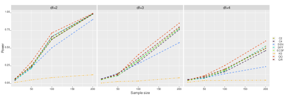
Figure 1: Power of the tests in Experiment (4.1) among 1000 simulated samples of different sizes (x-axis) for the different tests of Table 1 (colors). Each column represents the result for different degrees of freedom $df=2,3,4$ of the $t$ distribution.

The graphical interpretation of the global tests for $df=3$ and different test statistics are shown in Figure 2. The corresponding results for $df$ = 2 and $df$ = 4 are similar and hence are not shown. The QR test rejects the null hypothesis due to differences between the two distributions in extreme quantiles indicating distributional differences in the tails for $\tau<0.2$ and $\tau>0.7$. In this test, the first sample, i.e., the sample from the normal distribution is used as a reference category, and hence the empirical statistic corresponds to the coefficient of the second sample, i.e., the student-$t$ distributed sample. The test indicates that the smallest values in the second sample are significantly smaller than the expected values under the reference category, while the largest values in the second sample are larger than the expected values under the reference category. The QQ test rejects the null hypothesis for $\mid x\mid>1$. The small quantiles ($x<-1$) of the $t$-distributed sample are significantly smaller than the quantiles expected under the null hypothesis (1). Similarly, the large quantiles ($x>1$) of the $t$-distributed sample are significantly larger than the quantiles expected under the null hypothesis. These observations indicate that the distribution of the second sample has heavier tails than the distribution of the first sample.

The DIFF test also rejects the null hypothesis for $\mid x\mid>1$. Here, the test statistic $\mathbf{T}^{\text{diff}}$ is negative, i.e., $\widehat{F}_{2}(x)>\widehat{F}_{1}(x)$ for $x<-1$, and positive, i.e., $\widehat{F}_{2}(x)<\widehat{F}_{1}(x)$ for $x>1$. The same observation can be established from the ECDF test, where the second element of $\mathbf{T}^{\text{ecdf}}$ is shown. Thus, both test outputs indicate that the proportion of data with small values ($x<-1$) in the second sample is larger than the proportion of small values under the null hypothesis and there are more data in the second sample with large values ($x>1$) than what is expected under the null hypothesis. The DEN test shows that the second sample has higher density for $\mid x\mid>2$, as well as lower density for some $\mid x\mid<1$. These observations indicate that the distribution of the second sample has heavier tails than what is expected under the null hypothesis.

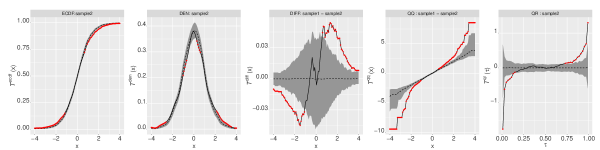
Figure 2: Graphical interpretation of the global tests in Experiment (4.1) with $N=1000$. The solid curve represents the empirical test statistic $\mathbf{T}_{0}$ while the dashed line shows the expected values of the test statistic under the null hypothesis (see Equation (1)). The shaded areas are the $95\%$ global envelopes constructed from 5000 permutations using the ERL measure. The points where $\mathbf{T}_{0}$ goes outside the global envelope are shown in red color. Each column shows the result of the global tests for the test statistic indicated in the titles (see Table 1). For the ECDF and DEN tests, only the second element of the test statistic is shown.

4.2 Mean shift

In Experiment (4.2), we studied the performance of the tests, when the two distributions differ only in the mean. In this case, the two samples are obtained as follows

$$\left\{\begin{array}[]{ll}X_{i}\sim\mathcal{N}(0,1)&\text{for }i=1,\ldots,N\\ Y_{i}\sim\mathcal{N}(0.3,1)&\text{for }i=1,\ldots,N\end{array}\right.$$

In such a case, it is well known that the asymptotic KS test is powerful. On the other hand, the KS test was outperformed by the majority of the global tests (Figure 3). Overall, the QR test was the most powerful. As in Experiment (4.1), the DEN test had the lowest power.

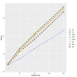
Figure 3: Power of the tests in Experiment (4.2) among 1000 simulated samples of different sizes (x-axis) for the different tests of Table 1 (colors).

The graphical interpretation of the tests for different test statistics is displayed in Figure 4. Due to large sample size, all tests clearly reject the null hypotheses (the empirical test statistic is outside the 95% global envelope for any value of $x$ or $\tau$), but with different reasoning. In the QR test we observe a significant (almost) constant positive quantile effect, i.e., $\widehat{\beta}(\tau)=0.3$ for most of the $\tau$ considered. Similarly, the QQ test rejects the null hypothesis for all $x$ considered. The empirical statistic is shifted uniformly from the line $y=x$, indicating that all values of the second sample are larger than the expected values under the null hypothesis. These observations, indicate that the two distributions differ by a location shift.

The DIFF test also rejects the null hypothesis for all $x$ considered. The test statistic is positive for all $x$ and therefore $\widehat{F}_{2}(x)<\widehat{F}_{1}(x)$ for all $x$. The same conclusion is derived from investigating the results of the ECDF test. According to the Figure 4, the ECDF of the second sample is shifted to the right compared to the mean ECDF of the two samples under the null hypothesis. This indicates that for a given $x\in[-2,2]$ we observe fewer data points smaller than $x$ than what is expected to be observed if the null hypothesis is true. Similarly, the DEN test shows that the second sample has a density that is shifted to the right compared to the expected mean density under the null hypothesis.

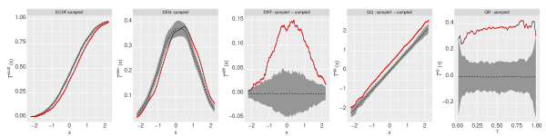
Figure 4: Graphical interpretation of the global tests in Experiment (4.2) with $N=1000$. The solid curve represents the empirical test statistic $\mathbf{T}_{0}$ while the dashed line shows the expected values of the test statistic under the null hypothesis (see Equation (1)). The shaded areas are the $95\%$ global envelopes constructed from 5000 permutations using the ERL measure. The points where $\mathbf{T}_{0}$ goes outside the global envelope are shown in red color. Each column shows the result of the global tests for the test statistic indicated in the titles (see Table 1). For the ECDF and DEN tests, only the second element of the test statistic is shown.

4.3 Variance shift

In Experiment (4.3), we studied the performance of the tests, when the two distributions differ only in the variance. In this case, the two samples are obtained as follows

$$\left\{\begin{array}[]{ll}X_{i}\sim\mathcal{N}(0,1)&\text{for }i=1,\ldots,N\\ Y_{i}\sim\mathcal{N}(0,1.3)&\text{for }i=1,\ldots,N\end{array}\right.$$

As seen in Figure 5, the asymptotic KS test had lower power than the proposed global envelope tests. The QQ test had the highest power while the ECDF test had the lowest power. Overall, the differences between the global tests with different test statistics were rather small.

The graphical interpretation of the tests for different test statistics is displayed in Figure 6. The graphical interpretation of the variance shift is rather similar to the difference in the tails case, except for the fact that the variance shift shows the departures from the null hypothesis on longer domains.

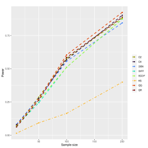
Figure 5: Power of the tests in Experiment (4.3) among 1000 simulated samples of different sizes (x-axis) for the different tests of Table 1 (colors).

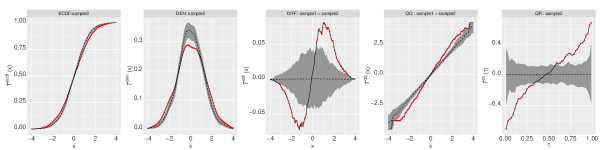
Figure 6: Graphical interpretation of the global tests in Experiment (4.3) with $N=1000$. The solid curve represents the empirical test statistic $\mathbf{T}_{0}$ while the dashed line shows the expected values of the test statistic under the null hypothesis (see Equation (1)). The shaded areas are the $95\%$ global envelopes constructed from 5000 permutations using the ERL measure. The points where $\mathbf{T}_{0}$ goes outside the global envelope are shown in red color. Each column shows the result of the global tests for the test statistic indicated in the titles (see Table 1). For the ECDF and DEN tests, only the second element of the test statistic is shown.

4.4 Mixture of normals

In Experiment (4.4), we studied the performance of the tests when one of the distributions is given as a mixture of two normal distributions and the other is the standard normal distribution. In this case, the two samples are obtained as follows

$$\left\{\begin{array}[]{ll}X_{i}\sim\mathcal{N}(0,1)&\text{for }i=1,\ldots,N\\ Z_{i}\sim\text{Bernoulli(0.5)}&\text{for }i=1,\ldots,N\\ Y_{i}=Z_{i}\cdot\mathcal{N}(1,0.5)+(1-Z_{i})\cdot\mathcal{N}(-1,0.5)&\text{for }i=1,\ldots,N\end{array}\right.$$

Unlike the results in the earlier sections, the DEN test was the most powerful test (see Figure 7). However, it is worth mentioning that the combined global envelope tests that consider the $\mathbf{T}^{\text{den}}$ statistic have similar performance. On the other hand, the QQ test had the lowest statistical power.

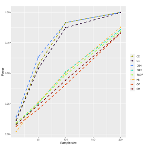
Figure 7: Power of the tests in Experiment (4.4) among 1000 simulated samples of different sizes (x-axis) for the different tests of Table 1 (colors).

The graphical interpretation of the tests for different test statistics is displayed in Figure 8. In the QR test, we observe an S-shaped empirical statistic. This indicates that the quantile effect of the group covariate varies across the whole distribution. In particular, there is a significant negative quantile effect for $\tau\in[0.1,0.4]$, indicating that the $\tau$-quantiles of the second sample for $\tau\in[0.1,0.4]$ are smaller than the respective $\tau$-quantiles of the first sample. Further, there is a significant positive quantile effect for $\tau\in[0.6,0.9]$, indicating that the $\tau$-quantiles of the second sample for $\tau\in[0.6,0.9]$ are larger than the respective $\tau$-quantiles of the first sample. The graphical interpretation of the QQ test shows an S-shaped pattern as well. The second sample’s quantiles $x\in[-1,0]$ are smaller and the second sample’s quantiles $x\in[0,1]$ are larger than the quantiles expected under the null hypothesis.

For the DIFF test, we observe an S-shape pattern indicating that $\widehat{F}_{2}(x)>\widehat{F}_{1}(x)$ for $x\in[-1.5,0)$, and $\widehat{F}_{2}(x)<\widehat{F}_{1}(x)$ for $x\in(0,1.5]$. The results are also similar for the ECDF test. Finally, the DEN test provides a straightforward interpretation, that is the distribution of the second sample is a bimodal distribution (second plot of Figure 8) and the distribution of the first sample is symmetric around 0 (third plot), and both of them are completely different than the mean behavior of the two samples under the null hypothesis of equal distributions.

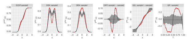
Figure 8: Graphical interpretation of the global tests in Experiment (4.4) with $N=1000$. The solid curve represents the empirical test statistic $\mathbf{T}_{0}$ while the dashed line shows the expected values of the test statistic under the null hypothesis (see Equation (1)). The shaded areas are the $95\%$ global envelopes constructed from 5000 permutations using the ERL measure. The points where $\mathbf{T}_{0}$ goes outside the global envelope are shown in red color. Each column shows the result of the global tests for the test statistic indicated in the titles (see Table 1). The second and third column together correspond to the two elements of the DEN test. For the ECDF test, only the second element of the test statistic is shown.

4.5 Skewness

In Experiment (4.5), we studied the performance of the tests when comparing a symmetrical distribution with a right-skewed distribution. In this case, the two samples were obtained as follows

$$\left\{\begin{array}[]{ll}X_{i}\sim\mathcal{N}(8,3.34)&\text{for }i=1,\ldots,N\\ Y_{i}\sim\text{log-normal(2,0.4)}&\text{for }i=1,\ldots,N\end{array}\right.$$

As seen in Figure 9, the proposed global envelope tests outperformed the asymptotic KS test in terms of power. The DEN test was the most powerful test for $N\leq 100$, while the QQ test was the most powerful for $N=200$. Overall, the combined global envelope tests performed quite well, even though they were outperformed by the aforementioned tests.

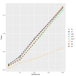
Figure 9: Power of the tests in Experiment (4.5) among 1000 simulated samples of different sizes (x-axis) for the different tests (colors).

The QR test rejects the null hypothesis for extreme quantiles $\tau<0.1$ and $\tau>0.9$ as well as for intermediate quantiles $\tau\in[0.35,0.75]$. There is a negative effect at the extreme quantiles indicating that the smallest and largest values of the log-normal sample are smaller than under the reference category of the quantile model, i.e., the first sample stemming from the normal distribution. Moreover, the quantile effect for $\tau\in[0.35,0.75]$ is positive indicating that the $\tau$-quantiles of the log-normal sample are larger than the respective $\tau$-quantiles under the reference category. Similarly, the QQ test rejects the null hypothesis for extreme quantiles $x<5$ and $x>15$ as well as for intermediate quantiles $x\in[7,10]$.

The DIFF test, indicates that $\widehat{F}_{2}(x)>\widehat{F}_{1}(x)$ for $x\in[0,5]\cup[13,16]$ and that $\widehat{F}_{2}(x)<\widehat{F}_{1}(x)$ for $x\in[7,10]$. The same conclusion can be established from the ECDF plot. The former result, suggests that the proportion of data with small ($x<5$) and large ($x>13$) values in the second sample is larger than the proportion expected under the null hypothesis. The latter suggests that in the second sample, there is a larger proportion of values in the interval [7,10] than what is expected under the null hypothesis. Last but not least, the DEN test shows that the distribution of the first sample is symmetric (third plot of Figure 10) while the distribution of the second sample is a right skewed distribution (second plot), and that both distributions are different from the distribution under the null hypothesis of equal distributions.

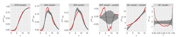
Figure 10: Graphical interpretation of the global tests in Experiment (4.5) with $N=1000$. The solid curve represents the empirical test statistic $\mathbf{T}_{0}$ while the dashed line shows the expected values of the test statistic under the null hypothesis (see Equation (1)). The shaded areas are the $95\%$ global envelopes constructed from 5000 permutations using the ERL measure. The points where $\mathbf{T}_{0}$ goes outside the global envelope are shown in red color. Each column shows the result of the global tests for the test statistic indicated in the titles (see Table 1). The second and third column together correspond to the two elements of the DEN test. For the ECDF, only the second element of the test statistic is shown.

4.6 Recommendations

The results from the simulation study indicated that the DEN test was slightly worse than the other tests in Experiments (4.1) and (4.2). On the other hand, in Experiment (4.4) the DEN, C2, and C4 tests were the most powerful. Finally, all proposed tests achieved similar performance in Experiments (4.3) and (4.5). The combined tests performed quite well in all examined cases, even though they were slightly outperformed by the best single test statistic-based tests in each scenario. As we typically do not know apriori how the distributions differ, we suggest using a combined test. Especially, we suggest using the $\text{C}2$ test as in most cases either the DEN or the QQ test was the most powerful. Moreover, this test provides a helpful graphical interpretation in each case as differences in the tails, location, or variances are well captured by the QQ test, and differences in the number of modes and location of the mode (skewness) are well captured by the DEN test. However, for $n$-sample comparisons with large $n$, we recommend using either the DEN, the QR, or the ECDF tests as their graphical interpretation includes only $n$ plots, while for the other tests the number of plots scale with $\mathcal{O}(n^{2})$.

5 Data Examples

5.1 Berkeley growth data

The Berkeley growth dataset (Tuddenham, 1954) includes height measurements from 39 boys and 54 girls from the first year of their life until adulthood and is available in the R package fda (Ramsay, 2023). Here, we are interested in investigating the hypothesis of equality between the height distributions of the two genders at different ages. For this purpose, we used the $\text{C}2$ test, i.e., a combined global envelope test with test statistics $\mathbf{T}^{\text{qq}}$ and $\mathbf{T}^{\text{den}}$.

Regarding the height distributions of the two genders at the age of 10 the test suggests that there is not enough evidence to reject the null hypothesis of equality of the two distributions ($p=0.348$). A graphical interpretation of the test result is presented in Figure 11. The empirical test statistics are fully contained within the $95\%$ global envelopes indicating that the height distributions of boys and girls at the age of 10 are the same.

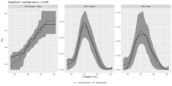
Figure 11: Graphical interpretation of the combined global envelope test for height distributions of boys and girls at the age of 10.

Further, we applied the same test to compare the height distributions of the two genders at the age of 14. According to our results, the height distributions of the two genders are different ($p=0.02$, Figure 12). The graphical interpretation of the test allows us to characterize this difference: There is a significantly higher proportion of boys with a height higher than 175 cm and a significantly lower proportion of girls with a height higher than 175 cm than what is expected under the null hypothesis. This is proven both by $\mathbf{T}^{\text{qq}}$ and $\mathbf{T}^{\text{den}}$. This indicates that at the age of 14, there are more tall boys than tall girls.

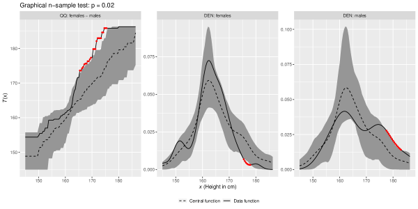
Figure 12: Graphical interpretation of the combined global envelope test for height distributions of boys and girls at the age of 14.

5.2 Iris data

The iris dataset includes flower characteristics from 50 flowers from three flower species (Anderson, 1935; Fisher, 1936). The flower species under study are the iris setosa, the iris virginica, and the iris versicolor. For each flower, measurements of the sepal length, sepal width, petal length, and petal width are available. Here, we investigated distributional differences of the sepal length distributions between the three flower groups.

For this purpose, we used the $\text{C}2$ test with $n=3$, i.e., the combined global envelope test with test statistics $\mathbf{T}^{\text{qq}}$ (see Equations (18) and (19)) and $\mathbf{T}^{\text{den}}$ (see Equations (10) and (17)) and $n=3$. Then, a combined test (see Section 2.5) is constructed based on the test vector

$$\mathbf{T}=(\mathbf{T}^{\text{qq}},\mathbf{T}^{\text{den}}).$$

The test rejects the null hypothesis of equality of the sepal length distributions of the three groups ($p<0.001$, Figure 13). Moreover, the test provides a graphical interpretation of the result which can be used to characterize the distributional differences between each pair of groups (see Section 3). All deviation patterns are similar to the one shown in Figure 4. Thus we can conclude that the differences are mostly in the mean only.

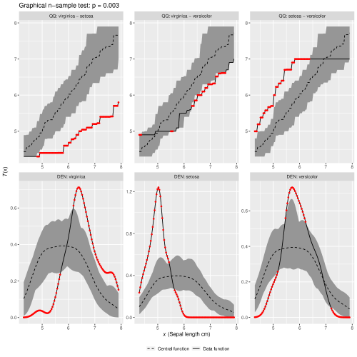
Figure 13: Graphical interpretation of the combined global envelope test for the sepal lengths distributions of three flower species (setosa, virginica and versicolor).

6 Discussion

In this paper, we proposed non-parametric, permutation-based tests for comparing the distribution of $n$ samples. The tests are based on the global envelope testing procedure which was introduced by Myllymäki et al. (2017) to solve the multiple testing problem in spatial statistics. The tests not only provide a Monte Carlo $p$-value but also provide a graphical interpretation of the test result. This allows the user to investigate the reason for rejecting the null hypothesis and get useful insights into the data at hand. The test is global in the sense that the test is performed simultaneously for all discrete values of the discretization of the test statistic, as well as all test statistics (the case of combined tests) and all group comparisons (the case of $n$ samples) made. That is, given a prespecified global significance level $\alpha$, a global envelope test constructs an acceptance region by controlling the family-wise error rate. Recently, methods for constructing the acceptance region by controlling the false discovery rate instead of the family-wise error rate were proposed by Mrkvička and Myllymäki (2023). It is useful for identifying all differences between the distributions since it is designed for local testing under the control of the expected number of false discoveries.

The proposed framework is generic and can be applied to any functional or multivariate test statistic $\mathbf{T}$ as the tests are based on ranks. That is, the test achieves the correct nominal level independently of the distribution of the test statistics. The only assumption needed is the exchangeability of the test statistics under the method used to simulate data under the null model. Here, we used a simple permutation scheme to simulate new data; that is, the observations of the variable of interest were permuted between the samples. The exchangeability assumption is satisfied for this permutation strategy.

We conducted a simulation study where we investigated the power of the proposed testing procedure with different test statistics capturing different aspects of the underlying distributions. We considered five test statistics as well as some combinations of them. The tests were applied to the two-sample cases under different simulated scenarios. In each scenario, a different distributional difference was investigated. Moreover, in each simulated experiment, we provide guidelines on how one should interpret the test results for the different proposed test statistics.

The statistical power of the global tests was compared to the power of the asymptotic Kolmogorov-Smirnov test, as this test also provides a graphical interpretation of the test result. Overall, the proposed tests outperformed the classical Kolmogorov-Smirnov test as they achieved higher statistical power in all studied settings. Even though the combined tests performed quite well in all simulated experiments, they were slightly outperformed by the best global tests based on single statistics. However, usually in real applications, distributional differences are apriori non-characterized, and therefore, using a combined test is suggested. The combined test also brings a wider graphical interpretation.

Last but not least, we demonstrated how the proposed tests can be applied to real data examples. For this purpose, we considered two datasets, the iris dataset and the Berkeley growth dataset. For the Berkeley growth data, we applied a combined global envelope test and compared the height distributions between the boys and girls at different ages. For the iris data, we applied a combined global envelope test and investigated whether there are distributional differences between the sepal length distributions of three flower species. In the future, we aim to investigate whether the proposed tests can be generalized to the case in which nuisance covariates are present with influence on the distribution of the variable under study. This problem is already solved for the quantile regression test statistic using the framework suggested by Mrkvička et al. (2023), but remains unsolved for a generic test statistic. The suggested procedure utilizes more sophisticated permutation strategies to remove the nuisance effects from the response distribution.

Appendix A: Type I errors

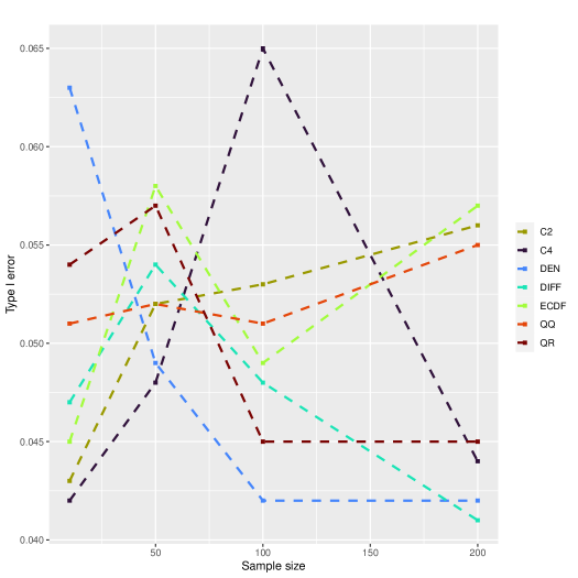
Figure 14: Type I errors of the tests among 1000 simulated standard normal samples of different sizes (x-axis) for the different tests of Table 1 (colors).

References

- Abdi (2010) Abdi, H. (2010). Holm’s sequential Bonferroni procedure. Encyclopedia of research design 1(8), 1–8.
- Aldor-Noiman et al. (2013) Aldor-Noiman, S., L. D. Brown, A. Buja, W. Rolke, and R. A. Stine (2013, November). The Power to See: A New Graphical Test of Normality. The American Statistician 67(4), 249–260. Publisher: Taylor & Francis _eprint: https://doi.org/10.1080/00031305.2013.847865.
- Anderson (1935) Anderson, E. (1935). The irises of the gaspe peninsula. Bulletin of American Iris Society 59, 2–5.
- Anderson and Darling (1954) Anderson, T. W. and D. A. Darling (1954). A test of goodness of fit. Journal of the American statistical association 49(268), 765–769.
- Cha (2007) Cha, S.-H. (2007). Comprehensive survey on distance/similarity measures between probability density functions. City 1(2), 1.
- Cramér (1928) Cramér, H. (1928). On the composition of elementary errors: First paper: Mathematical deductions. Scandinavian Actuarial Journal 1928(1), 13–74.
- Doksum and Sievers (1976) Doksum, K. A. and G. L. Sievers (1976). Plotting with confidence: Graphical comparisons of two populations. Biometrika 63(3), 421–434.
- Dowd (2020) Dowd, C. (2020). A new ecdf two-sample test statistic. arXiv preprint arXiv:2007.01360.
- Dowd (2023) Dowd, C. (2023). twosamples: Fast Permutation Based Two Sample Tests. https://twosampletest.com, https://github.com/cdowd/twosamples.
- Fisher (1936) Fisher, R. A. (1936). The use of multiple measurements in taxonomic problems. Annals of eugenics 7(2), 179–188.
- Gilleland and Katz (2016) Gilleland, E. and R. W. Katz (2016). extRemes 2.0: An extreme value analysis package in R. Journal of Statistical Software 72(8), 1–39.
- Hahn (2015) Hahn, U. (2015). A note on simultaneous monte carlo tests. Technical report, Centre for Stochastic Geometry and advanced Bioimaging, Aarhus University.
- Hajk-Georg (2018) Hajk-Georg, D. (2018). Philentropy: Information theory and distance quantification with R. Journal of Open Source Software 3(26), 765.
- Holm (1979) Holm, S. (1979). A simple sequentially rejective multiple test procedure. Scandinavian journal of statistics, 65–70.
- Koenker and Bassett Jr (1978) Koenker, R. and G. Bassett Jr (1978). Regression quantiles. Econometrica: journal of the Econometric Society, 33–50.
- Kolmogorov (1933) Kolmogorov, A. (1933). Sulla determinazione empirica di una lgge di distribuzione. Inst. Ital. Attuari, Giorn. 4, 83–91.
- Kuiper (1960) Kuiper, N. H. (1960). Tests concerning random points on a circle. In Nederl. Akad. Wetensch. Proc. Ser. A, Volume 63, pp. 38–47.
- Lehmann et al. (1986) Lehmann, E. L., J. P. Romano, and G. Casella (1986). Testing statistical hypotheses, Volume 3. Springer.
- Mrkvička et al. (2023) Mrkvička, T., K. Konstantinou, M. Kuronen, and M. Myllymäki (2023). Global quantile regression. arXiv preprint arXiv:2309.04746.
- Mrkvička and Myllymäki (2023) Mrkvička, T. and M. Myllymäki (2023). False discovery rate envelopes. Statistics and Computing 33(5), 109.
- Mrkvička et al. (2022) Mrkvička, T., M. Myllymäki, M. Kuronen, and N. N. Narisetty (2022). New methods for multiple testing in permutation inference for the general linear model. Statistics in Medicine 41(2), 276–297.
- Mrkvička et al. (2020) Mrkvička, T., M. Myllymäki, M. Jílek, and U. Hahn (2020). A one-way ANOVA test for functional data with graphical interpretation. Kybernetika 56(3), 432–458.
- Mrkvička et al. (2021) Mrkvička, T., M. Myllymäki, M. Kuronen, and N. N. Narisetty (2021). New methods for multiple testing in permutation inference for the general linear model. Statistics in Medicine.
- Myllymäki and Mrkvička (2023) Myllymäki, M. and T. Mrkvička (2023). GET: Global envelopes in R. arXiv:1911.06583 [stat.ME].
- Myllymäki et al. (2017) Myllymäki, M., T. Mrkvička, H. Seijo, P. Grabarnik, and U. Hahn (2017). Global envelope tests for spatial processes. Journal of the Royal Statistical Society: Series B (Statistical Methodology) 79(2), 381–404.
- Narisetty and Nair (2016) Narisetty, N. N. and V. J. Nair (2016). Extremal depth for functional data and applications. Journal of the American Statistical Association 111(516), 1705–1714.
- Praestgaard (1995) Praestgaard, J. T. (1995). Permutation and bootstrap kolmogorov-smirnov tests for the equality of two distributions. Scandinavian Journal of Statistics, 305–322.
- R Core Team (2023) R Core Team (2023). R: A Language and Environment for Statistical Computing. Vienna, Austria: R Foundation for Statistical Computing.
- Ramsay (2023) Ramsay, J. (2023). fda: Functional Data Analysis. R package version 6.1.4.
- Ripley (1981) Ripley, B. D. (1981). Spatial Statistics. Wiley Series in Probability and Mathematical Statistics. New Jersey: John Wiley & Sons, Inc.
- Shaphiro and Wilk (1965) Shaphiro, S. and M. Wilk (1965). An analysis of variance test for normality. Biometrika 52(3), 591–611.
- Silverman (2018) Silverman, B. W. (2018). Density estimation for statistics and data analysis. Routledge.
- Smirnov (1948) Smirnov, N. (1948). Table for estimating the goodness of fit of empirical distributions. The annals of mathematical statistics 19(2), 279–281.
- Tuddenham (1954) Tuddenham, R. D. (1954). Physical growth of california boys and girls from birth to eighteen years. University of California publications in child development 1(2).
- Vaserstein (1969) Vaserstein, L. N. (1969). Markov processes over denumerable products of spaces, describing large systems of automata. Problemy Peredachi Informatsii 5(3), 64–72.
- Warton (2022) Warton, D. I. (2022). Eco-stats: data analysis in ecology: from t-tests to multivariate abundances. Springer Nature.