Dynamics of quantum observables and Born’s rule in Bohmian Quantum Mechanics

Abstract

In the present paper we study both ordered and chaotic Bohmian trajectories in the Born distribution of 2d quantum systems. We find theoretically and numerically the average values of the energy, momentum, angular momentum and position of 2d quantum systems. In particular, we consider realizations of the Born distribution of a system with a single nodal point and of two different cases with many nodal points, one with almost equal number of ordered and chaotic trajectories and one consisting of almost exclusively chaotic trajectories. The numerical average values agree with the theoretical values if the Born $P=|\Psi|^{2}$ rule is initially satisfied, but do not agree when $P_{0}\neq|\Psi_{0}|^{2}$. We study the role of ordered and chaotic trajectories in providing these average values.

Introduction

Bohmian Quantum Mechanics (BQM) [1, 2, 3] is a basic alternative interpretation of Quantum Mechanics. Contrary to standard Quantum Mechanics (SQM) [4, 5, 6], in BQM the quantum particles follow deterministic trajectories in spacetime, which are guided by the wavefunction describing the system, i.e. the solution of the Schrödinger equation:

$$-\frac{\hbar^{2}}{2m}\nabla^{2}\Psi+V\Psi=i\hbar\frac{\partial{\Psi}}{\partial t},$$ (1)

according to the so called “Bohmian equations of motion”:

$$m\frac{dr}{dt}=\hbar\Im\left(\frac{\nabla\Psi}{\Psi}\right).$$ (2)

Thus the state of a quantum system in BQM is described by its wavefunction and the positions of it associated Bohmian particles in the configuration space.

BQM predicts the same experimental results as SQM, when the Bohmian particles are distributed according to Born’s rule (BR), which states that the probability density of finding a quantum particle in a certain region of space is equal to $P=|\Psi|^{2}$. If BR is initially satisfied then it is easily proved that it will be satisfied for all times. However, in BQM we are allowed to consider initial configurations of Bohmian particles distributed with $P_{0}\neq|\Psi_{0}|^{2}$. Whether BR will be accesible in the long run in such cases is a fundamental problem in BQM and it has been shown that it depends strongly on the complexity of the Bohmian trajectories [7, 8, 9].

In particular the highly nonlinear character of the Bohmian equations of motion allows the coexistence of ordered and chaotic Bohmian trajectories for a given quantum system, where order/chaos refers to the low/high sensitivity of the trajectories on the initial conditions. Thus BQM allows the study of chaotic dynamics in the quantum framework by use of all the techniques of the theory of classical dynamical systems, something that has been the main topic of many works in the past [10, 11, 12, 13, 14, 15, 16, 17, 18, 19, 20, 21, 22].

In our series of works on Bohmian chaos we showed that the nodal points of the wavefunction $\Psi$ (i.e. the points where $\Psi=0$) are essential for the production of chaos. In fact in the frame of reference of a moving nodal point $N$ there is an unstable fixed point, the ‘X-point’. Together they form the so called ‘nodal point-X-point complexes’. When a Bohmian particle comes close to an NPXPC it gets deflected by the X-point. The effect of many such encounters is the emergence of chaos. Furthermore in a recent paper [23] we showed that there are also unstable points in the inertial frame of reference, the ‘Y-points’ that play some role in the generation of chaos. Trajectories that never approach X-points or Y-points are in general ordered.

The study of the mechanism responsible for chaos production was crucial for understanding the role of order and chaos in the accessibility of BR by arbitrary initial distributions of Bohmian particles. In [24, 25] we showed that the BR distribution contains in general both chaotic and ordered trajectories. The chaotic trajectories of a given system were found to have a common footprint on the configuration space, i.e. their points acquire a common long time distribution regardless of their initial condition. Thus they are ergodic (or partially ergodic). However, the corresponding long time distributions of points of ordered trajectories cover limited regions of the configuration space. Thus we found that BR will be accessible only by initial distributions with the correct proportion between ordered and chaotic trajectories, and the correct distribution of ordered trajectories. Moreover, the number of ordered trajectories in the BR distribution may not be negligible even in the case of systems with multiple nodal points. Consequently, the common belief that a large number of nodal points guarantees the accessibility of Born’s rule is in general not valid.

After all the above studies in the dynamics of Bohmian trajectories, it is reasonable for one to ask what is the role of the ordered and chaotic trajectories in producing the correct observed average values of observables, when $P_{0}=|\Psi_{0}|^{2}$. This is the subject of the present paper, where we consider a number of 2d wavefunctions and we calculate the average values of the energy, the momentum $(p_{x},p_{y})$, the angular momentum $L$ and the position $(x,y)$ of a large number of Bohmian particles, sampled according to the Born distribution. These values are compared with the corresponding theoretical values predicted by standard quantum mechanics. By counting the numbers of ordered and chaotic trajectories in the Born distribution of these wavefunctions we examine their contribution in the observed average values.

In order to simplify our calculations we have taken the quantum systems corresponding to a simple ordered classical system, that of two harmonic oscillators $V=\frac{1}{2}(\omega_{x}^{2}x^{2}+\omega_{y}^{2}y^{2}$). In this case the solutions of the Schrödinger equation are given analytically and the theoretical values of the various quantities are calculated analytically as well. Details of these calculations are given in the Appendix.

We have taken various cases of $\Psi$, as superpositions of 3 stationary states. In particular, we have an example with a single nodal point (Section 2) and two examples with many nodal points (Section 3), one with equal proportions of ordered and chaotic trajectories and one example where chaotic trajectories dominate the BR distribution. In Section 4 we make our summary and comment on our results.

Wavefunction with a single node

We consider first a wavefunction with a single nodal point:

$$\Psi=M(a\Psi_{00}+b\Psi_{10}+c\Psi_{11}).$$ (3)

where $\Psi_{m,n}(x,y)=\Psi_{m}(x)\Psi_{n}(y)$. $\Psi_{m}(x)$ and $\Psi_{n}(y)$ are the 1-D energy eigenstates of the oscillator in $x$ and $y$ coordinates correspondingly, i.e.

$$\Psi_{m,n}=\prod_{q=x}^{y}N_{q}\exp\left(-\frac{\omega_{q}q^{2}}{2\hbar}\right)\exp\left(-\frac{i}{\hbar}E_{s}t\right)H_{s}\left(\sqrt{\frac{M_{q}\omega_{q}}{\hbar}}q\right),$$ (4)

where $s=m,n$ (integers) for $x$ and $y$ respectively and the normalization constant is $N_{q}=\frac{(M_{q}\omega_{q})^{\frac{1}{4}}}{\pi\hbar\sqrt{2^{s}s!}}$. The functions $H_{m},H_{n}$ are Hermite polynomials in $\sqrt{\frac{M_{x}\omega_{x}}{\hbar}}x$ and $\sqrt{\frac{M_{y}\omega_{y}}{\hbar}}y$ of degrees $m$ and $n$ respectively and $E_{s}=\left(s+\frac{1}{2}\right)\hbar\omega_{q}$.

In this case we have only one nodal point (the equations $\Psi_{R}=\Psi_{Im}=0$ are of first degree in $x$ and $y$). In Fig. 1 we show the Born distribution $P=\Psi|^{2}$ made out of 5000 particles, when $M_{x}=M_{y}=1,\hbar=1,a=b=1,c=\sqrt{2}/2,\omega_{x}=1,\omega_{y}=\sqrt{2}/2$. The value of the normalizing constant $M$ is found by setting $M^{2}(a^{2}+b^{2}+c^{2})=1$. It is $M=\sqrt{2/5}$. The red points represent the initial conditions which produce ordered trajectories and the blue points the initial conditions of chaotic trajectories. We observe that the ordered trajectories dominate the BR distribution (almost 97%). The chaotic trajectories ($3\%$) start in regions of small $P=|\Psi|^{2}$ at the boundaries of the two blobs as shown in the plane $(x,y)$ (Fig. 1b). Chaos appears when a trajectory approaches the region of the nodal point.

The maximum value of $P$ in the main blob is $P\simeq 0.33$ and in the second blob it is $P\simeq 0.06$. In Fig. 1c we give the colorplot of the distribution, i.e. the density on the $(x,y)$ plane of the points of the trajectories at every $\Delta t=0.05$ of the BR distribution in a quadratic grid of bins up to a certain time $t$. Here we show the colorplot at $t=0$. It is clear that the maxima correspond to the tops of the two blobs and $P$ decreases outwards.

Then we calculate the theoretical average value of energies which is [6]

$$\langle E\rangle=M^{2}(|a|^{2}E_{00}+|b|^{2}E_{10}+|c|^{2}E_{11}),$$ (5)

where

$$E_{m,n}=(m+1/2)\hbar\omega_{x}+(n+1/2)\hbar\omega_{y}.$$ (6)

We remind that since $\Psi_{m,n}$ are eigenstates of the quantum harmonic oscillator. $\langle E\rangle$ is constant in time. In the present case we find $\langle E\rangle=1.595$.

On the other hand, the average values of the energy $E_{av}$ of the Bohmian particles depend on their sampling in the realization of the Born distribution. Each particle has a total energy

$$E=K+V+Q,$$ (7)

where $K$ is the kinetic energy $\frac{1}{2}(\dot{x}^{2}+\dot{y}^{2})$, $V$ is the potential energy $V=\frac{1}{2}(\omega_{x}^{2}x^{2}+\omega_{y}^{2}y^{2})$ and $Q$ is the Bohmian quantum potential energy $Q=-\frac{1}{2}\frac{\nabla^{2}|\Psi|}{|\Psi|}$.

The trajectories are calculated by solving the Bohmian equations of motion, up to a certain time $t$. Examples of a chaotic and an ordered trajectory are shown in Figs. 2a,b.

In Fig. 3 we have taken the average value for numbers of particles $N=100,200,..13000$ and find the corresponding values of $E_{av}$ at $t=0$. These values show significant deviations from the theoretical value for small numbers of Bohmian particles but for $N>5000$ they approach the theoretical value.

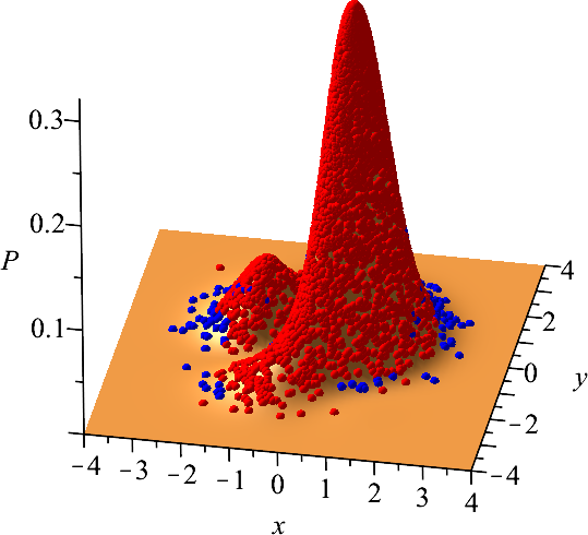
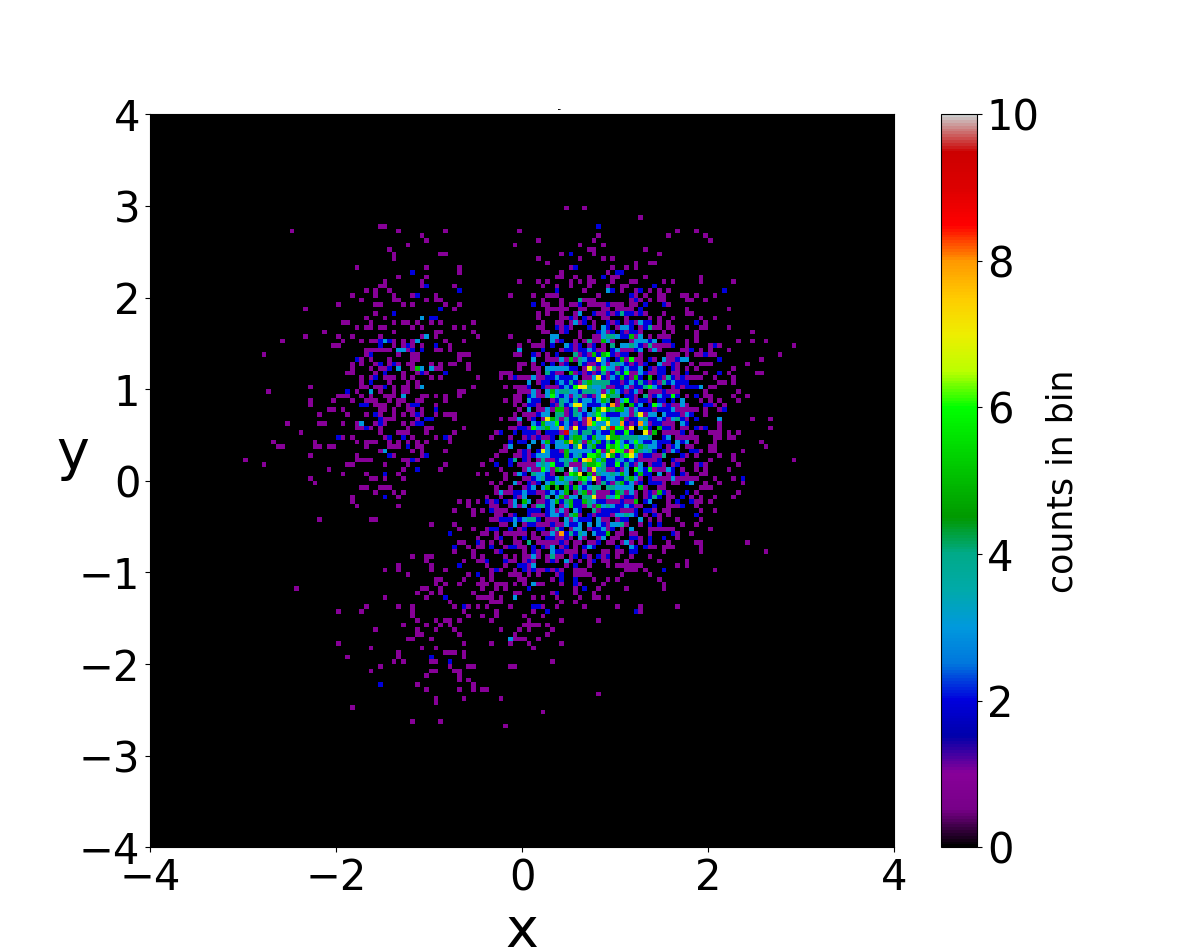
[a] [b] [c]

Figure 1: 5000 initial conditions of ordered (red) and chaotic (blue) trajectories distributed according to BR in the case of the wavefunction with a single nodal point. a) on the surface of $|\Psi|^{2}$ and b) on the $x-y$ plane. In c) we see their colorplot at $t=0$.

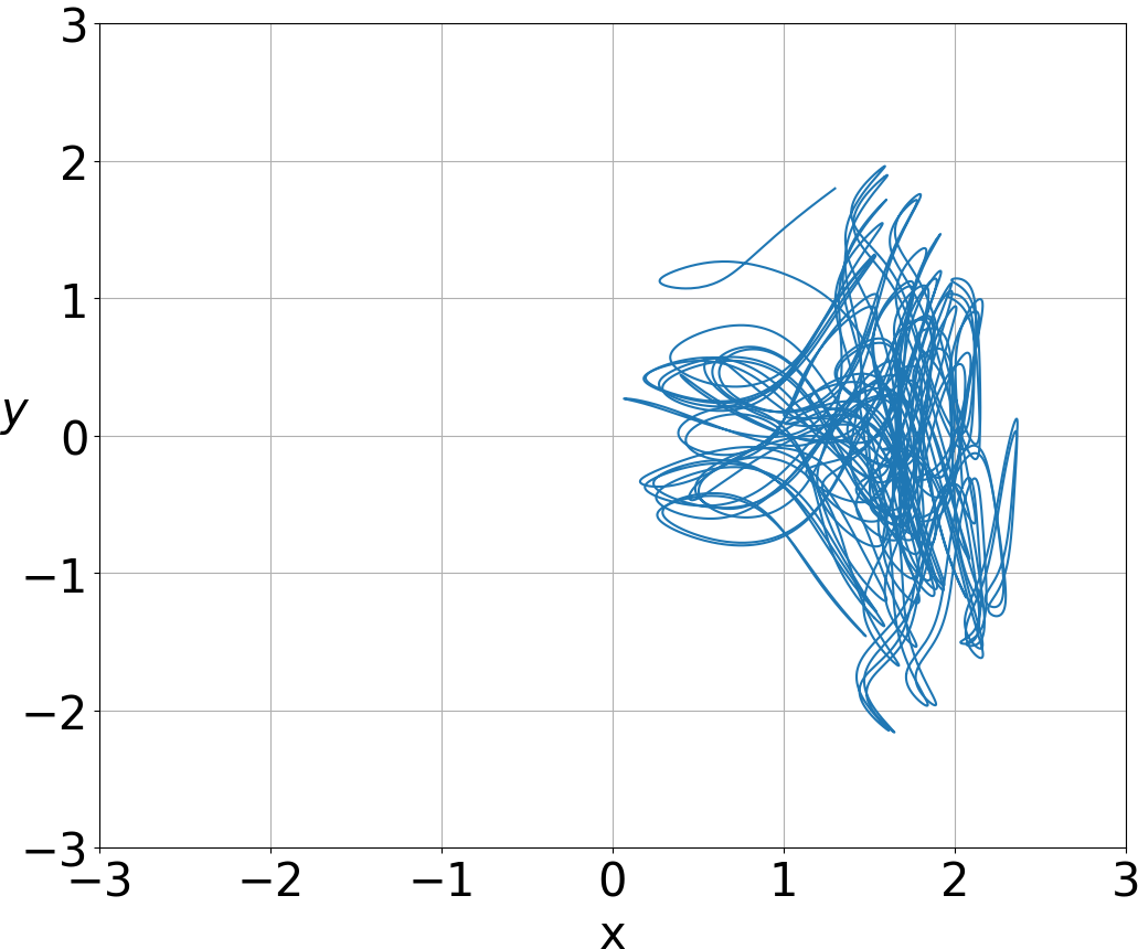
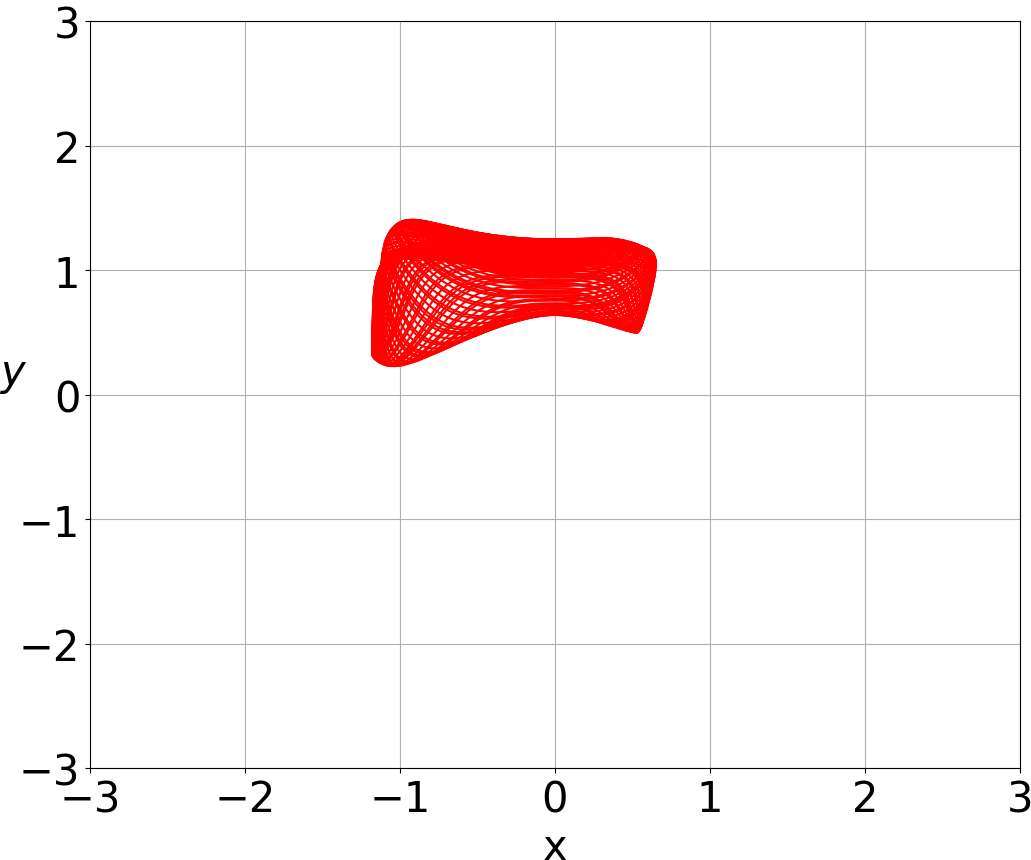
[a] [b]

Figure 2: A chaotic trajectory ($x(0)=1.3,y(0)=1.8$) (a) and an ordered trajectory ($x(0)=0.2,y(0)=1.0$) (b) in the case of the single node wavefunction.

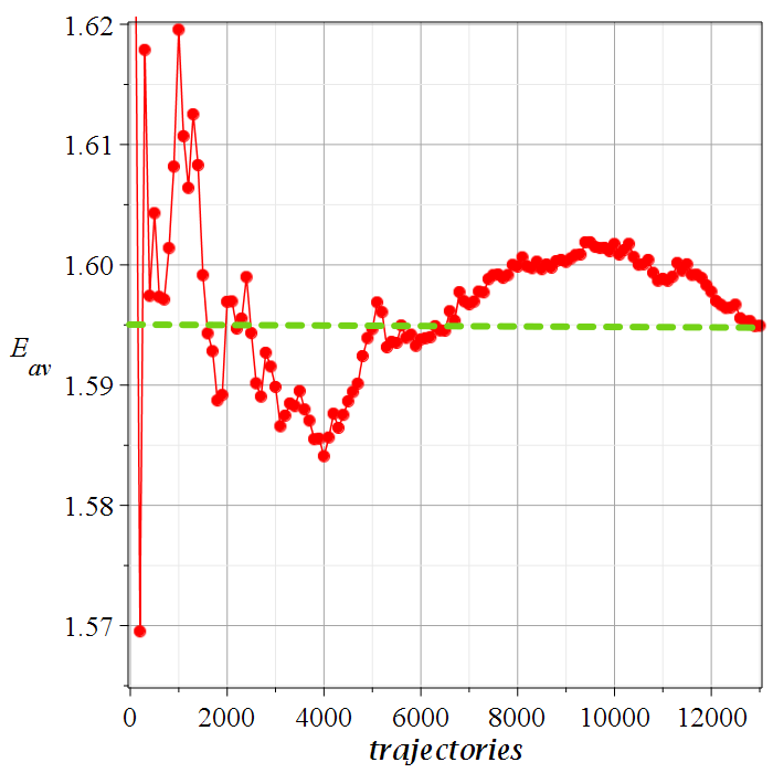
Figure 3: The average value of energy as a function of the number of particles in a realization of Born’s distribution for the wavefunction with a single nodal point.

For $N=5000$ the average value is close to $E_{av}=1.595$. But, in order to have a better estimation of $E_{av}$ we have considered 5 different (random) realizations of BR distribution with $N=5000$ Bohmian particles. Their average value at $t=0$ is $E_{av}(0)=1.599\pm 0.004$, i.e. it is a little above the theoretical value $\langle E\rangle$. If we integrate the trajectories of all realizations up to $t=1000$ then we find that the mean absolute deviation between the theoretical and the numerical values is $\sim 0.005$, i.e. we can write $E_{av}=\langle E\rangle\pm 0.005$. Thus $E_{av}$ has deviation from the theoretical value $\langle E\rangle=1.595$ of order about 3%. By taking larger numbers of particles we find a better approach to the theoretical value. We note that although the numerical value $E_{av}$ is calculated by a quite different method (the Bohmian equations of motion) than the theoretical value, the results are very close to each other.

On the other hand, in an initial distribution of particles different from Born’s rule we find quite different values of $E_{av}$. In a particular case with $P_{0}\neq|\Psi_{0}|^{2}$ we found $E_{av}=0.819,$ a value much smaller than $\langle E\rangle=1.595$.

Then we separated the initial Born distribution of Fig. 1 into various zones of extent $\Delta P=0.03$. Namely, the zones 1,2,…11 contain the particles with P in the intervals $0<P<0.03,$ $0.03<P<0.06,...$ up to $0.3<P<0.33$. We calculated the contribution of the various zones in finding $E_{av}$ and in Fig. 4a we give the energy of the particles in every zone divided by the total number $N=5000$ of particles. We see that the zones 3,4,..10 contribute roughly equal amounts in $E_{av}$ namely $0.123\pm 0.015$. The last zone (11) contributes a little less (0.096) and the two first zones contribute about double the average (0.268 in zone 1 and 0.246 in zone 2). In these two zones the contribution of the particles of the second blob is manifest.

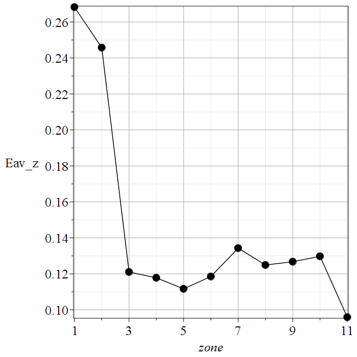
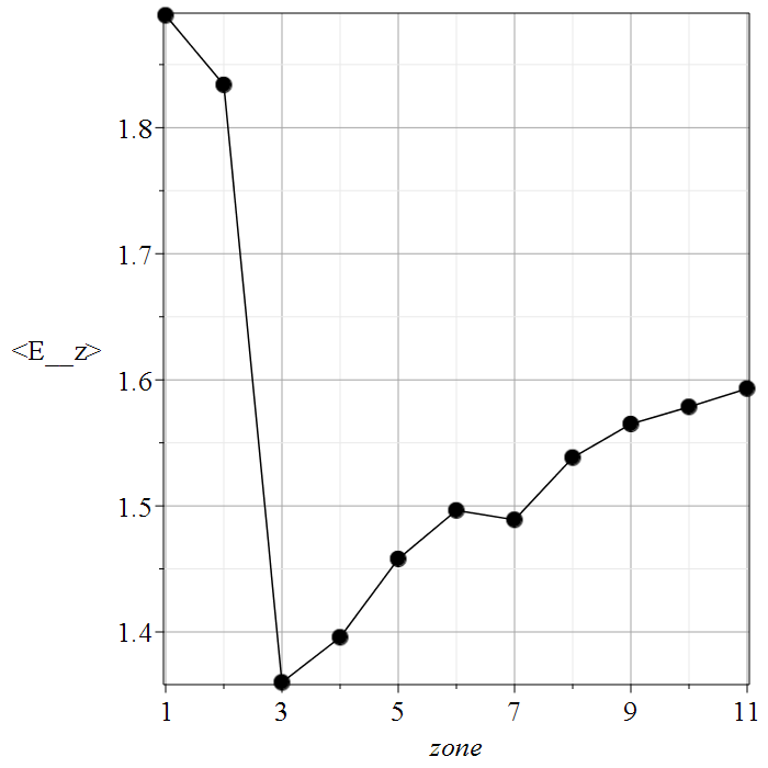
[a] [b]

Figure 4: (a) The contributions of the successive zones ($1-11$) to the total average of the energy $E_{av}$ at $t=0$ (b) The separate values of the energy $E_{av}$ in the various zones.

If we take the average energy in the various zones $1,2,\dots 11$ by dividing their contribution by the corresponding number of particles (and not by $5000$) we see that the average value of the last zone is $1.593$, very close to the global average (Fig. 4b). The previous zones ($10,9,\dots 3$) have decreasing values of $E_{av}$ except for the first two zones (2 and 1) which have very large values because of the second blob.

On the other hand, the chaotic trajectories are very close to the bottom of the distribution $(P=0)$ and their average values of $E_{av}$ is $1.58$, smaller than the theoretical value and very close to the minimum value of Fig. 4b. It is notable that the chaotic trajectories do not give average values close to the theoretical value. On the contrary the best approach is provided by the ordered trajectories on the top of the large blob of Fig. 1a. Thus the claim that the distribution of particles tends to the Born distribution because of the chaotic trajectories is not realized in the present case, first because the number of the chaotic trajectories is small and second because the chaotic trajectories in the present case do not give the correct average value of the energy. Therefore if we start with an initial distribution of only chaotic trajectories we will not reach the Born distribution in the long run. In fact, even if we keep the correct proportions of ordered/chaotic trajectories, we cannot reach the Born distribution unless the ordered trajectories have the distribution found within the Born rule. E.g. if we take initially ordered trajectories only from the top of the large blob we will not ever reach the Born distribution.

Besides the values of the energy it is of interest to find the average values of other basic quantum observables as well, such as the momentum, angular momentum and position.

The theoretical mean value of the $p_{x}$ component of the momentum is given by

$$\langle p_{x}\rangle=\int_{-\infty}^{\infty}\int_{-\infty}^{\infty}\Psi^{*}\hat{p}_{x}\Psi dxdy,$$ (8)

where $\hat{p}_{x}=-i\hbar\frac{\partial}{\partial x}$ is the corresponding momentum operator and $\Psi^{*}$ is the complex conjugate of $\Psi$. The analytical calculation of $\langle p_{x}\rangle$ is given in the Appendix. There we show the various terms of the function $\Psi^{\dagger}\hat{p}_{x}\Psi$ and indicate those terms that give nonzero contributions in the integrals (8). In the present case we find after some algebra

$$\langle p_{x}\rangle=-\frac{\sqrt{2\omega_{x}}ab\sin(\omega_{x}t)}{a^{2}+b^{2}+c^{2}}.$$ (9)

Therefore $\langle p_{x}\rangle$ is time dependent. Similarly we find that

$$\langle p_{y}\rangle=-\frac{\sqrt{2\omega_{y}}bc\sin(\omega_{y}t)}{a^{2}+b^{2}+c^{2}}.$$ (10)

In Fig. 5a we give the values of $\langle p_{x}\rangle$, which change with a period $T=2\pi$, up to $t=1000$. We have marked with red dots the values of $\langle p_{x}\rangle$ at every multiple of $t=50$. In every interval $\Delta t=50$ we have about 8 oscillations. If we calculate now the average values of $\langle p_{x}\rangle$ of 5000 particles at these times we find almost exactly the same values (blue dots) with a mean deviation in $p_{x}$ equal to $\sim 0.005$. Similar values are found in Fig. 5b for $\langle p_{y}\rangle$. The mean deviation in $p_{y}$ is $\sim 0.003$.

The theoretical angular momentum is

$$\langle L\rangle=\langle L_{z}\rangle =\int_{-\infty}^{\infty}\int_{-\infty}^{\infty}(\Psi^{*}x\hat{p_{y}}-y\hat{p}_{x})\Psi dxdy$$ (11)

$$={\frac{1}{\sqrt{\omega_{x}\omega_{y}}}}\frac{ac\left(\omega_{x}-\omega_{y}\right)\sin\left(\left(\omega_{x}+\omega_{y}\right)t\right)}{{a}^{2}+{b}^{2}+{c}^{2}}$$

and the theoretical average values $\langle x\rangle,\langle y\rangle$ are found equal to (see the Appendix for further details):

$$\langle x\rangle=\sqrt{\frac{2}{\omega_{x}}}\frac{ab\cos(\omega_{x}t)}{a^{2}+b^{2}+c^{2}}$$ (12)

$$\langle y\rangle=\sqrt{\frac{2}{\omega_{y}}}\frac{ab\cos(\omega_{y}t)}{a^{2}+b^{2}+c^{2}}.$$ (13)

We note that

$$\langle p_{x}\rangle=\frac{d\langle x\rangle}{dt},\,\langle p_{y}\rangle=\frac{d\langle y\rangle}{dt}.$$ (14)

In the present case for $t=0$ we have $\langle x\rangle=0.566$ and $\langle y\rangle=0.336$ while $\langle p_{x}(0)\rangle=\langle p_{y}(0)\rangle=0$. The mean deviations between the theoretical values and the numerical values of $\langle L\rangle$, $\langle x\rangle,\langle y\rangle$ for $t\in[0,1000]$ are $0.008$ $0.007$ and $0.010$ correspondingly.

For any arbitrary distribution of particles $P_{0}\neq|\Psi_{0}|^{2}$ the mean deviations of the numerical average values from the theoretical ones are in general large (see Table 1).

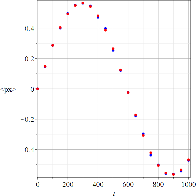
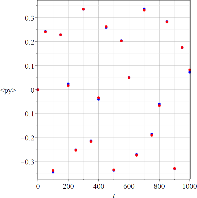
[a] [b]

Figure 5: The average values of $\langle p_{x}\rangle$ (a) and $\langle p_{y}\rangle$ (b) as functions of time for $t\in[0,1000]$ for every $\Delta t=50$. The red dots correspond to the theoretical values produced by Eqs. 6,7 and the blue dots correspond to the values produced by a realization of 5000 Bohmian particles distributed according to BR.

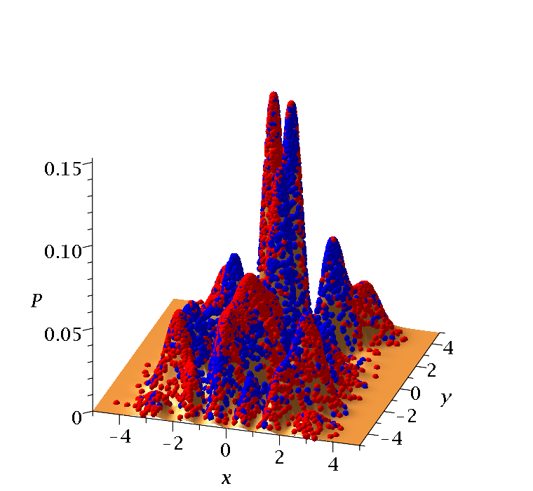
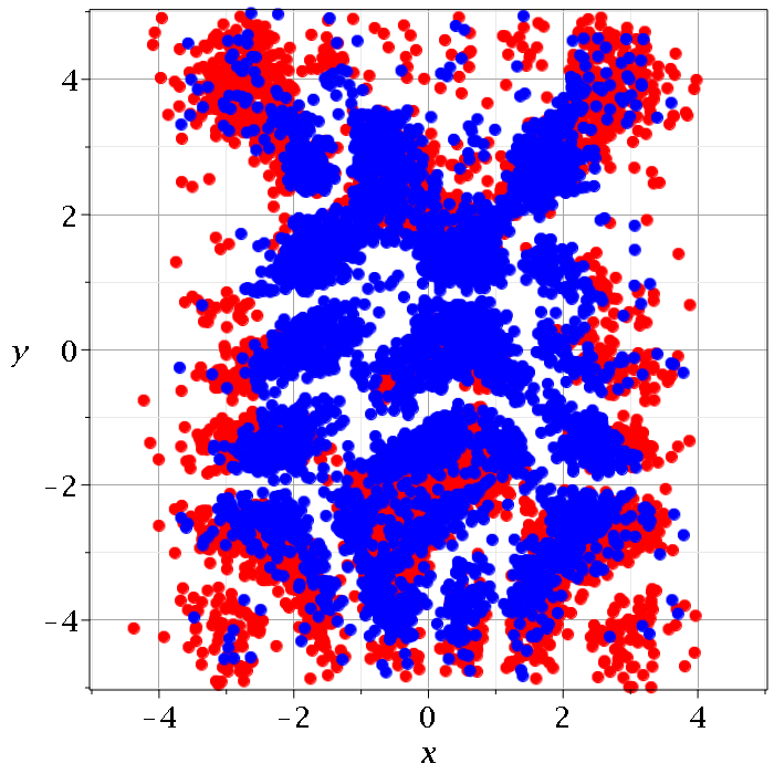
[a] [b]
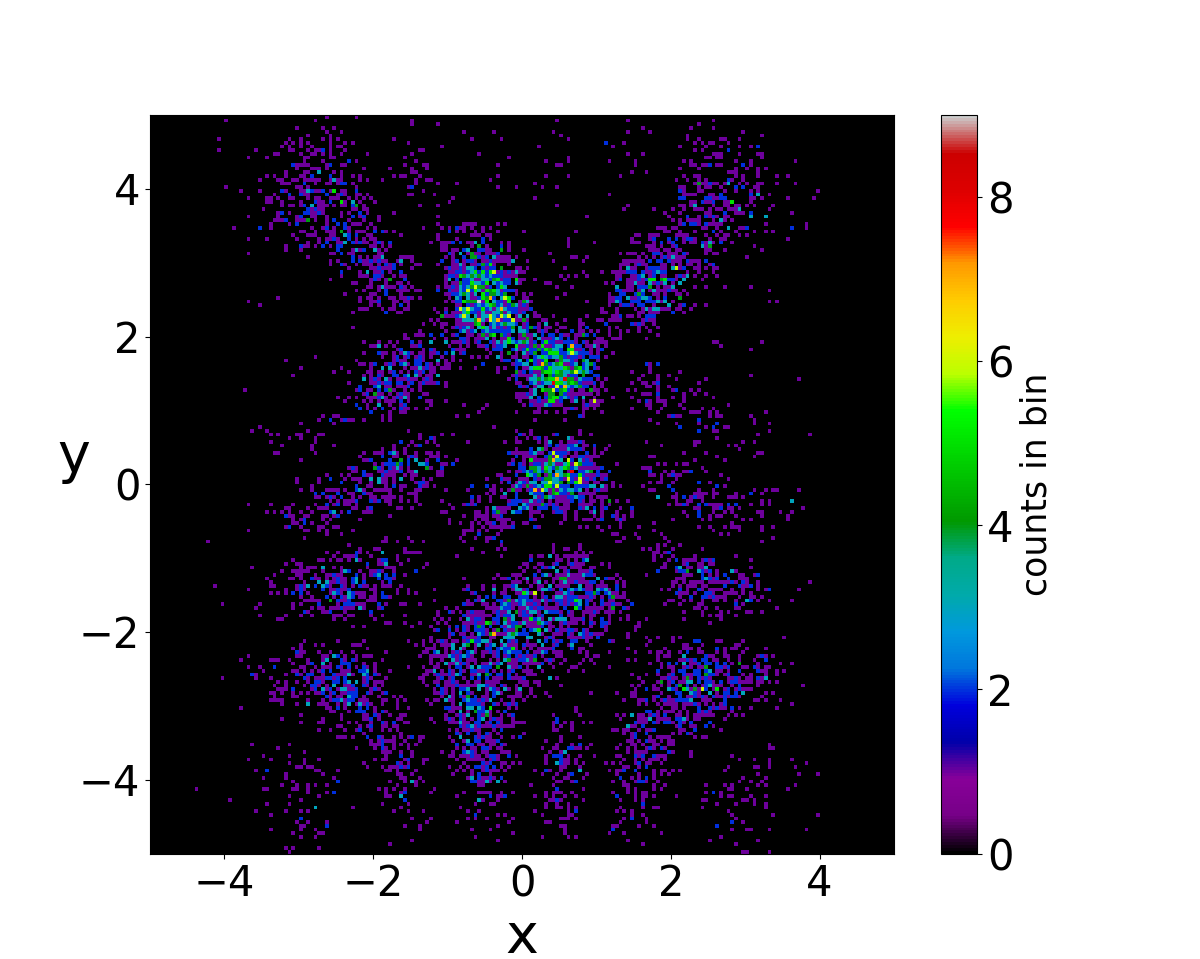
[c]

Figure 6: 10000 initial conditions of ordered (red) and chaotic (blue) trajectories distributed according to BR in the case of the wavefunction $\Psi=M(a\Psi_{0,2}+b\Psi_{3,4}+c\Psi_{5,7})$: a) on the surface of $P=|\Psi|^{2}$ and b) on the $x-y$ plane. In c) we see their colorplot at $t=0$.

Wavefunctions with many nodal points

Case 1

A wavefunction with many nodal points is

$$\Psi=M(a\Psi_{0,2}+b\Psi_{3,4}+c\Psi_{5,7}),$$ (15)

where the functions $\Psi_{m,n}$ are given by Eq. 4. The constants have the same values as in Section 2.

In this case the maximum $m_{i}$ is $5$ and the maximum $n_{i}$ is $7$, therefore the number of the nodal points is of order 35. An initial distribution of $10000$ particles is shown in Figs. 6a,b. It has many blobs that collide as they evolve in time. The proportions of ordered (red) and chaotic (blue) trajectories are in this case about 50%. Chaos is generated mainly when a particle approaches one of the nodal points (and its nearby X-point). The distribution of the particles at $t=0$ is shown in the initial colorplot (Fig. 6c).

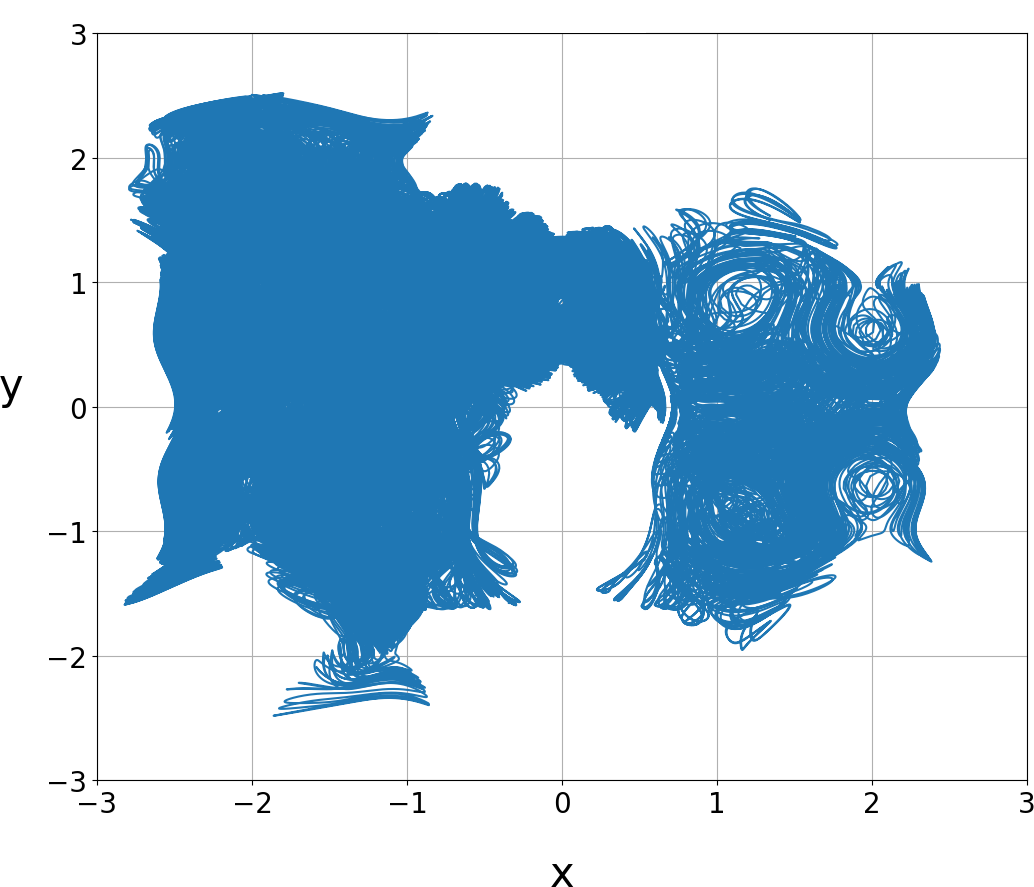
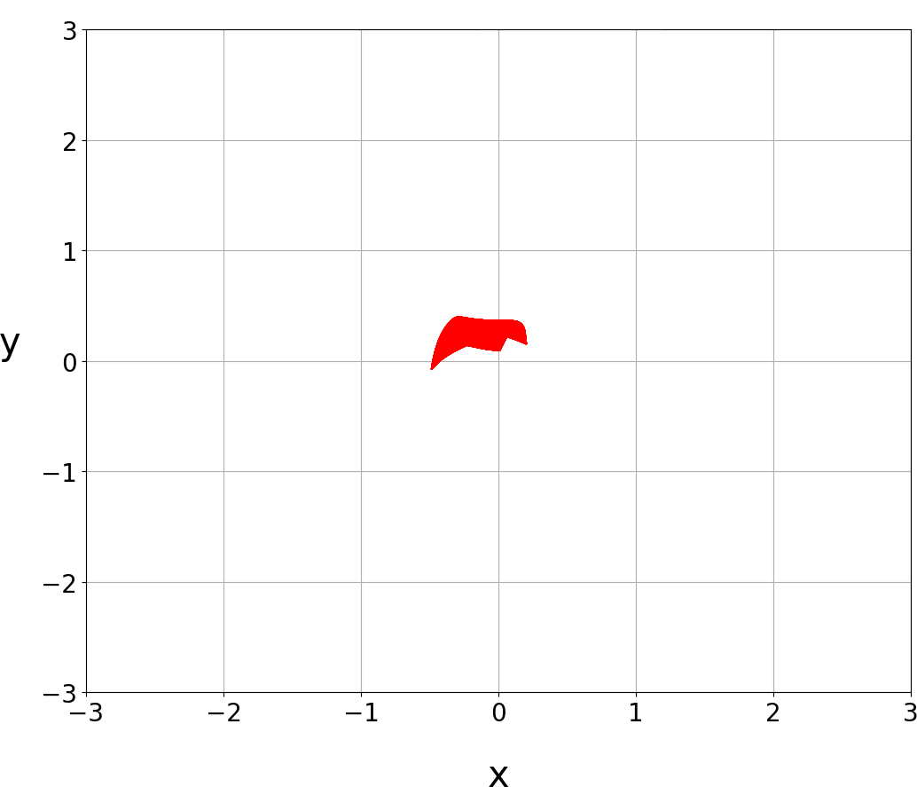
[a] [b]

Figure 7: a,b) A chaotic $(x(0)=-0.6,y(0)=-0.01)$ (a), and an ordered ($x(0)=0.01,y(0)=0.1$) trajectory (b), of the wavefunction $\Psi=M(a\Psi_{0,2}+b\Psi_{3,4}+c\Psi_{5,7})$.

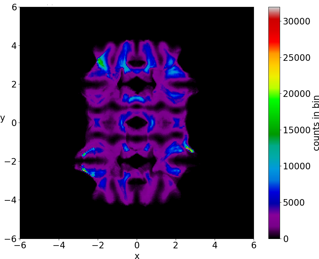
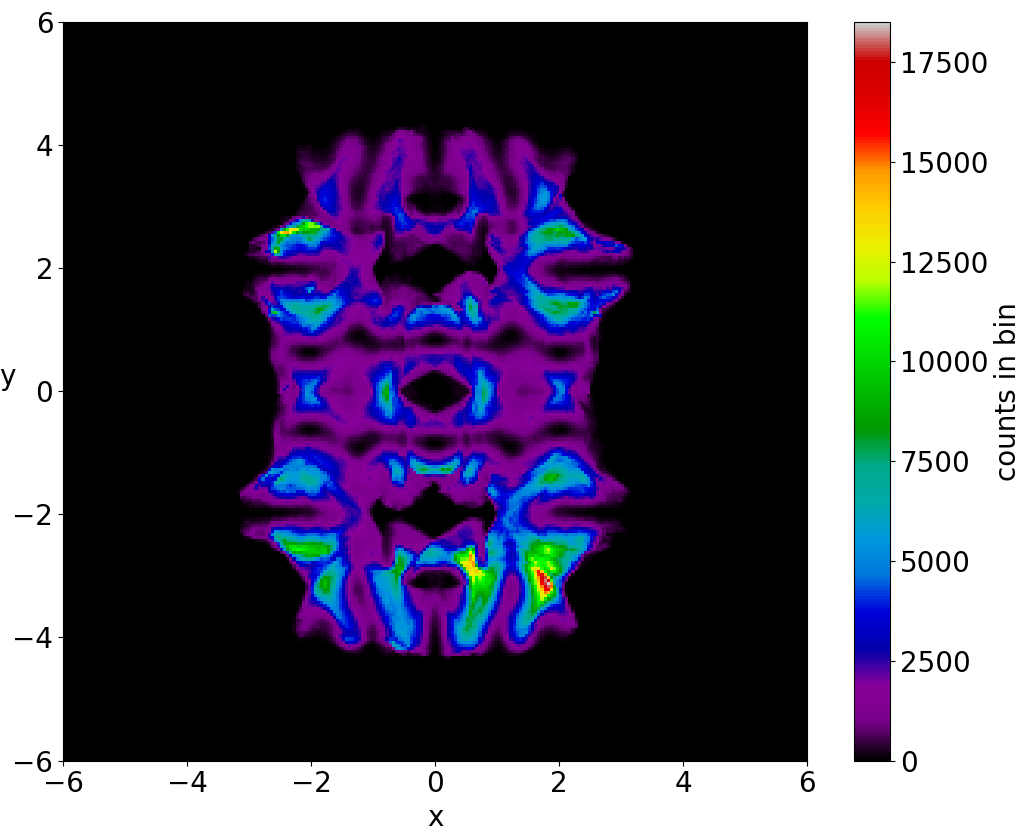
[a] [b]

Figure 8: The colorplots of two chaotic trajectories of the wavefunction $\Psi=M(a\Psi_{0,2}+b\Psi_{3,4}+c\Psi_{5,7})$ up to $t=2\times 10^{6}$: a) $x(0)=0.6693,y(0)=-2.4559$ b) $x(0)=-0.0631,y(0)=-1.4241$.

The ordered trajectories are mainly close to the tops of the two main blobs. This supports our previous results on qubit states [25, 26] made of coherent states of the quantum harmonic oscillator, where we found that the concentration of the ordered trajectories in the Born distribution is at the top of the larger of the two blobs of $|\Psi|^{2}$.

The forms of the the chaotic trajectories are very irregular (Fig. 7a), while the ordered trajectories are like distorted Lissajous figures (Fig. 7b). Moreover the chaotic trajectories are ergodic as we can see in Figs. 8a,b where we show two different chaotic trajectories having very similar colorplots (cumulative distributions of points taken at every $\Delta t=0.05$ up to $t=2\times 10^{6}$).

Figure 9: The colorplot of an ordered trajectory ($x(0)=0.01,y(0)=0.1$) up to $t=1000$. We see that it covers a very small area of the configuration space.

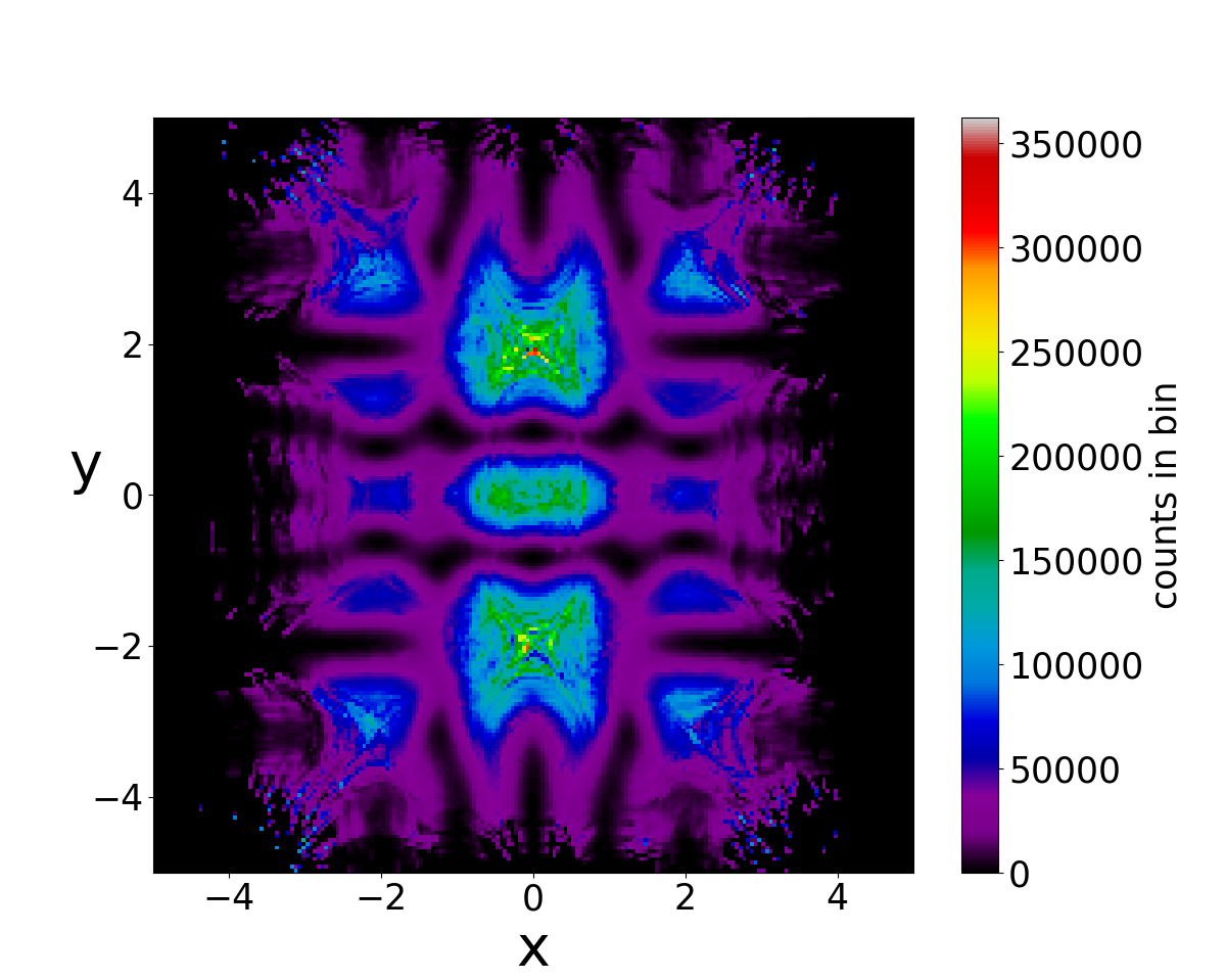
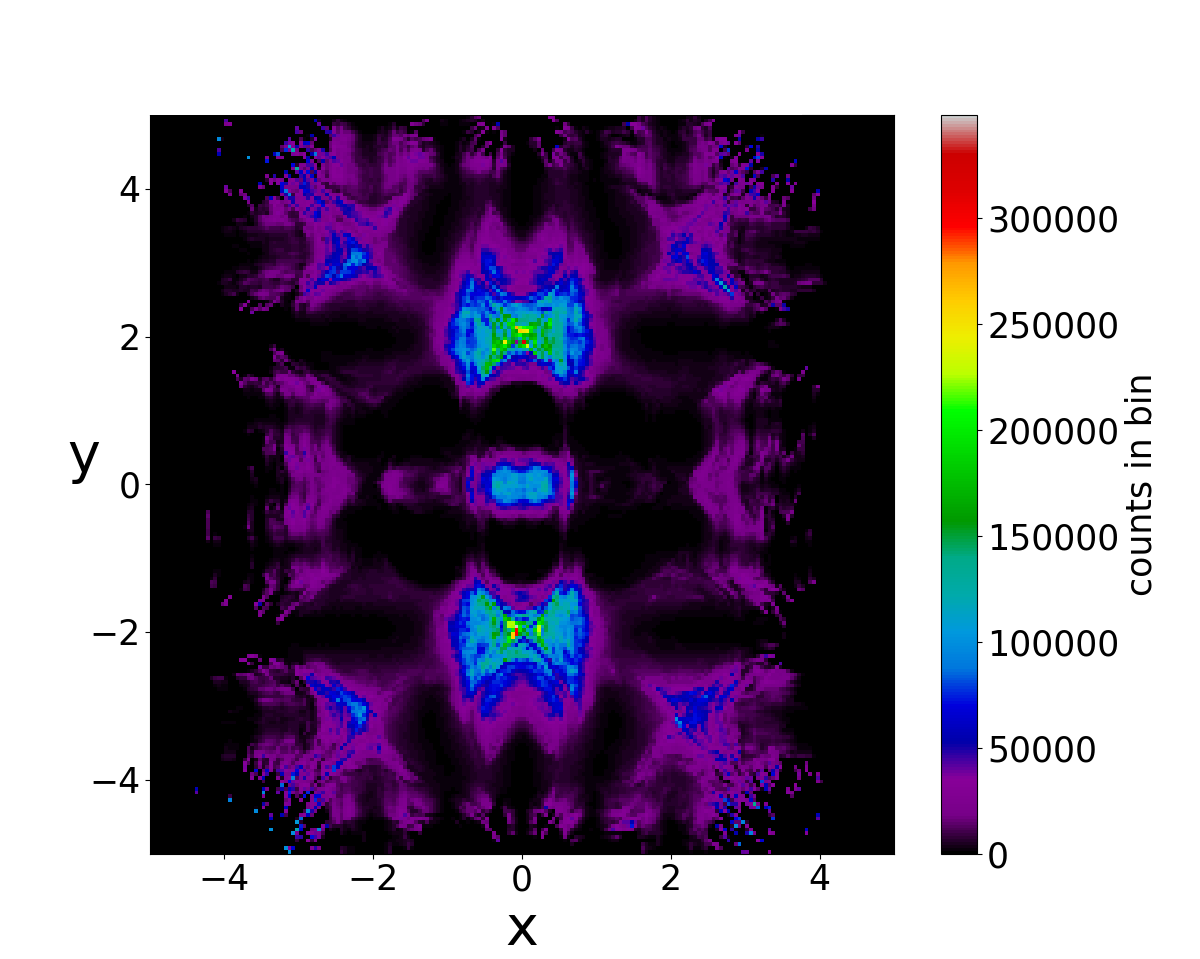
[a]
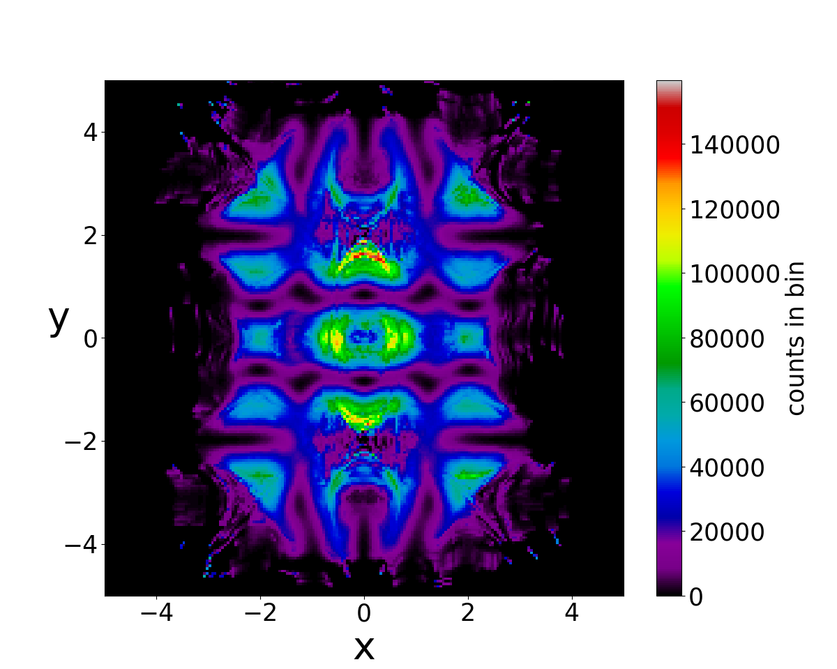
[b] [c]

Figure 10: a) The colorplot of a realization of BR distribution consisting of $10000$ particles integrated up to $t=5000$ in the case of the wavefunction $\Psi=M(a\Psi_{0,2}+b\Psi_{3,4}+c\Psi_{5,7})$. The colorplots of the $5053$ chaotic and $4947$ ordered trajectories are given separately in (b) and (c).

On the other hand the colorplots of ordered trajectories cover only a small part of the space $(x,y)$ (Fig. 9). Therefore their colorplots are very different from those of the chaotic trajectories.

In Fig. 10a we show the colorplot of all the particles up to a time $t=5000$, while the colorplots of the chaotic and of the ordered trajectories up to this time are shown in Figs. 10b,c. We see that the colorplots Figs. 10a,b,c are quite different from each other. Therefore, if we take only chaotic (or only ordered) trajectories we will never reach the Born distribution.

As regards the averages values of the observed quantities in this case we have the following: The theoretical average of the energies is

$$\langle E\rangle=M^{2}(|a|^{2}E_{0,2}+|b|^{2}E_{3,4}+|c|^{2}E_{5,7}),$$ (16)

where $E_{m,n}$ are given by Eq. 6. Using the values $a=b=1,c=\sqrt{2}/2$ and $M^{2}=(a^{2}+b^{2}+c^{2})^{-1}$ we find that $\langle E\rangle=5.7406$. Then we calculate the average value $E_{av}$ of $N=10000$ Bohmian particles we find that, at $t=0$, $\langle E\rangle=5.7438.$ Therefore the initial deviation is of order $0.003$, i.e. $0.06\%$.

The theoretical values of the momentum $\langle p_{x}\rangle,\langle p_{y}\rangle$, of the angular momentum $\langle L\rangle$ and of the position $\langle x\rangle$ $\langle y\rangle$ are calculated in the Appendix. In the present case they are all zero, i.e., $\langle p_{x}\rangle=\langle p_{y}\rangle=\langle L\rangle=\langle x\rangle=\langle y\rangle=0$. In fact, in the Appendix we show that they are zero whenever $m$ and $n$ differ by more than 1 (i.e. whenever they are not adjacent integers). The corresponding mean absolute deviations of $\langle p_{x}\rangle,\langle p_{y}\rangle$ for $10000$ Born distributed particles and $t\in[0,1000]$ are $0.009,0.007$. The corresponding values for the angular momentum $\langle L\rangle$ and the position $\langle x\rangle,\langle y\rangle$ are $0.0234$ and $0.0122$ and $0.0158$ (see Table 1).

On the other hand, in a case with $10000$ particles distributed randomly in the square $(-1,1)\times(-1,1)$, i.e. away from the BR distribution, we found much larger deviations for the same time, namely $0.29$ and $0.23$. These values are more than $3000$ times larger than the values of the Born distribution (see Table 1).

Case 2

If we take

$$\Psi=M(a\Psi_{10,3}+b\Psi_{4,5}+c\Psi_{7,8})$$ (17)

we have $m_{i}^{max}=10,n_{i}^{max}=8$, therefore the number of the nodal points is of order $N_{p}=80$. In this case the proportion of chaotic trajectories is about $96.2\%$ and the ordered trajectories are only $3.8\%$.

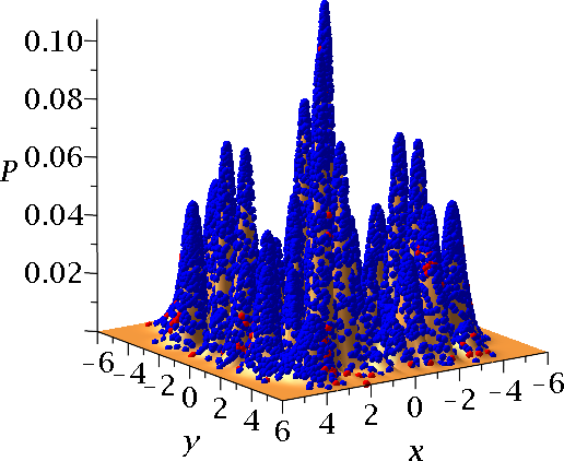
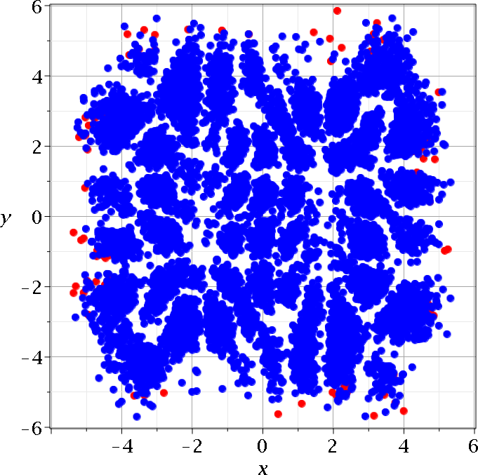
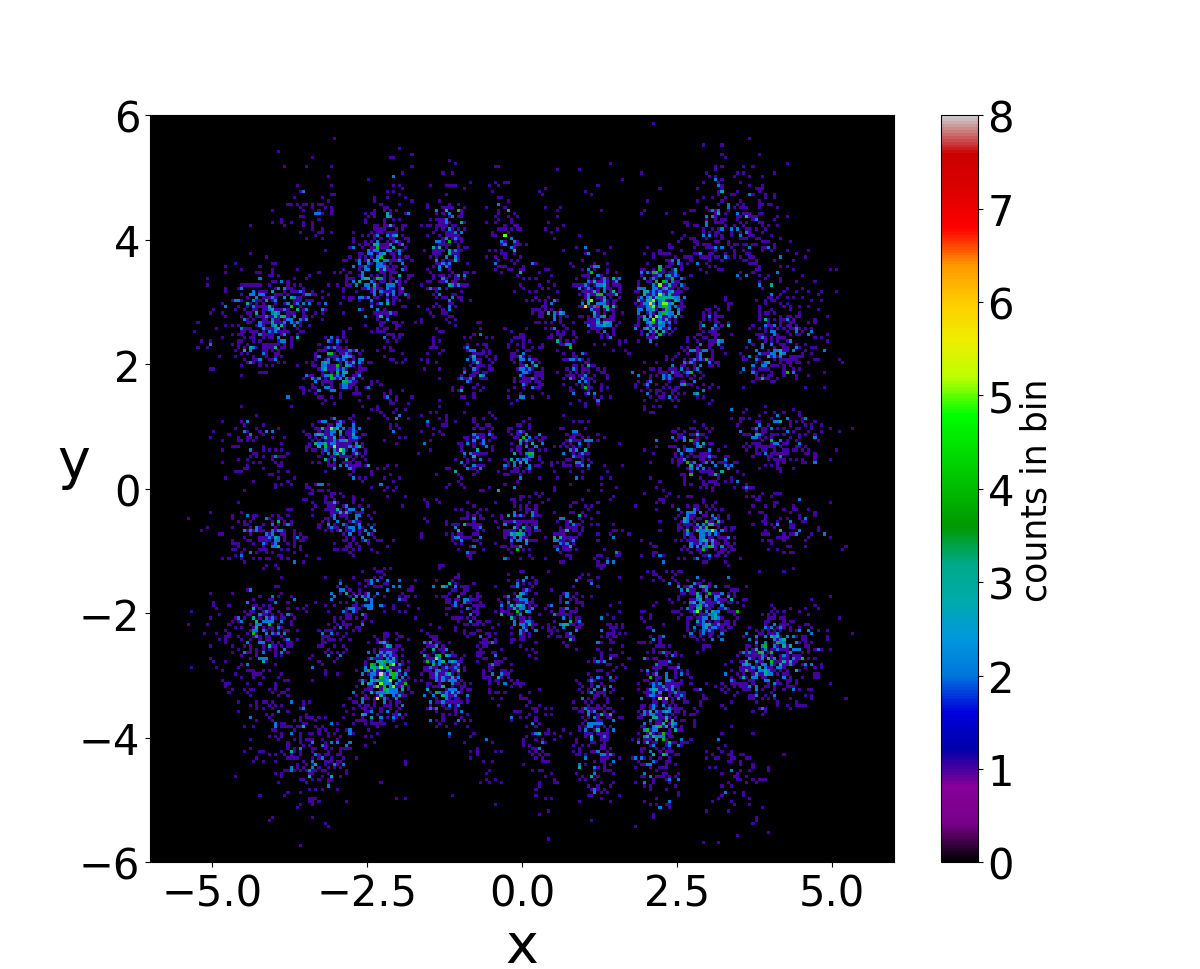
[a] [b] [c]

Figure 11: 10000 initial conditions of ordered (red) and chaotic (blue) trajectories distributed according to BR in the case of the wavefunction $\Psi=M(a\Psi_{10,3}+b\Psi_{4,5}+c\Psi_{7,8})$: a) on the surface of $P_{0}=|\Psi_{0}|^{2}$ and b) on the $x-y$ plane ($t=0$). c) Their colorplot at $t=0$.

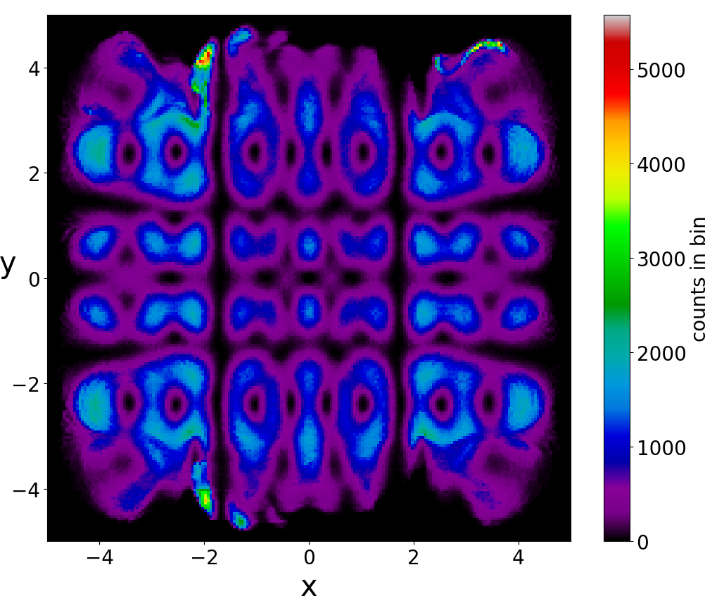
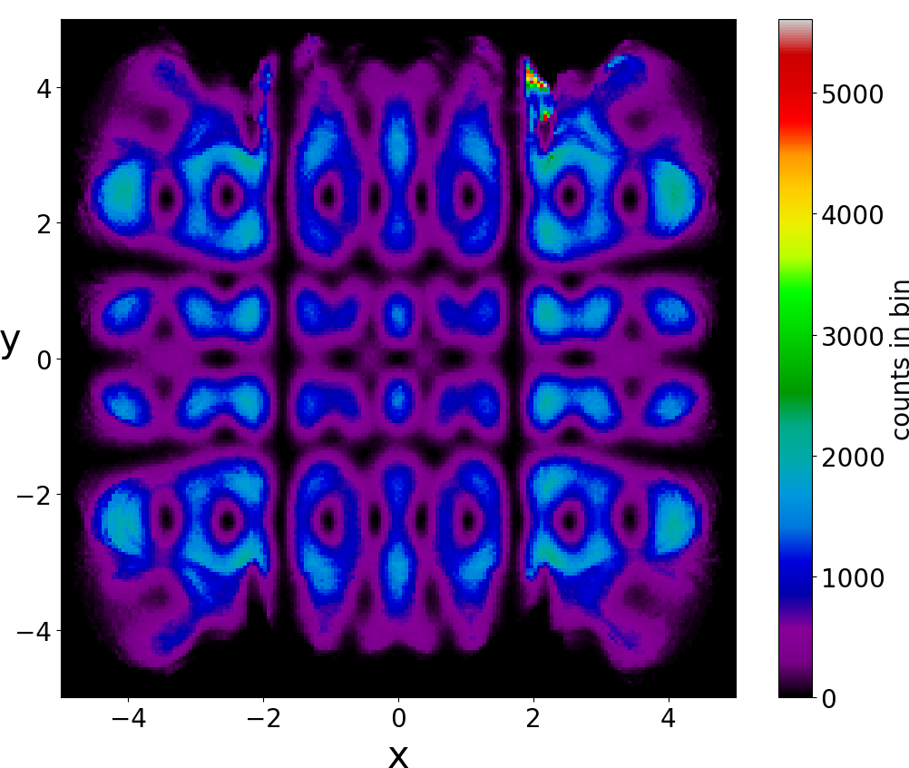
[a] [b]

Figure 12: The colorplot of two chaotic trajectories up to $t=10^{6}$ in the case $\Psi=M(a\Psi_{10,3}+b\Psi_{4,5}+c\Psi_{7,8})$: a) $x(0)=-1,y(0)=0.7$ and b) $x(0)=-0.1,y(0)=-1.5$. They look very similar.

The initial distributions of the points according to BR is given in Fig. 11. In this case the tops of the main blobs contain mainly chaotic trajectories, which in fact are ergodic. This is shown in Fig. 12 where we compare the colorplots of two chaotic trajectories up to $t=10^{6}$.

In particular, the theoretical average energy is $\langle E\rangle=M^{2}(a^{2}E_{10,3}+b^{2}E_{4,5}+|c|^{2}E_{7,8})$ and this is equal to $\langle E\rangle=11.248$. In Fig. 13 we show the numerical average at $t=0$ as a function of the number of particles in the Born distribution. We see that the numerical value converges to $E_{av}=11.239$ when the number $N$ is larger than $2000$. The errors are about $0.009$, i.e. of order $0.08\%$.

The theoretical average momenta $\langle p_{x}\rangle$ and $\langle p_{y}\rangle$, angular momentum $\langle L\rangle$ and position $\langle x\rangle,\langle y\rangle$ are zero (since the values of $m$ and $n$ are not different by 1, see the Appendix).

The mean absolute deviations in time are also found to be very close to zero. In particular the deviations $|\delta\langle p_{x}\rangle|_{av},|\delta\langle p_{y}\rangle|_{av}$ for 10000 particles following Born’s distribution and for $t\in[0,1000]$ are 0.0082 and 0.0081. In this case the variations of a random non-Born distribution in the square $(-1,1)\times(-1,1)$ (taken the same as in the case 3.1) are $0.011$ and $0.013$, i.e. of the same order as for an initially Born distribution (see Table 1). This is due to the fact that any non Born distribution tends to reach BR distribution in the long run when it is dominated by chaotic-ergodic trajectories.

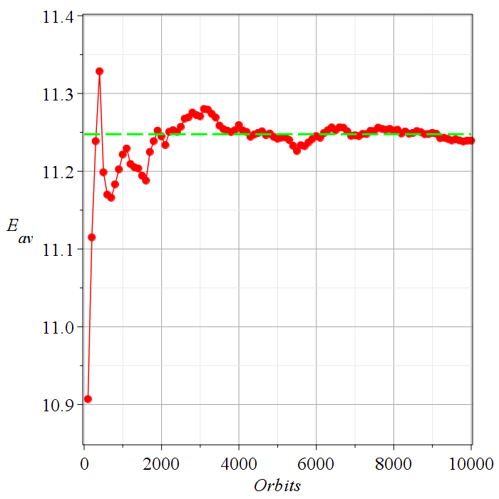
Figure 13: The average value of energy as a function of the number of trajectories in the realization of Born’s rule at $t=0$.

Conclusions

In this paper we have considered mainly distributions of particles that satisfy Born’s rule $P=|\Psi|^{2}$. In general Born’s distribution contains both chaotic and ordered trajectorie and the chaotic trajectories are ergodic or partially ergodic.

In the case of one nodal point the ordered trajectories are dominant. In the first case of many nodal points the ordered trajectories are almost equal to the chaotic trajectories, while in the second case the chaotic trajectories are dominant. In this case the Born distribution is essentially satisfied in the long run, even if the initial distribution is not Born-distributed.

However the existence of many nodal points does not necessarily imply that chaos is dominant. In fact, there are special cases of multinodal wavefunctions which are dominated by ordered trajectories. Nevertheless these cases are rather exceptional.

We calculated the average values of the observed quantities, namely the energy $\langle E\rangle$, the momentum $\langle p_{x}\rangle,\langle p_{y}\rangle$, the angular momentum $\langle L\rangle$ and the position $\langle x\rangle,\langle y\rangle$. The theoretical values are found analytically in the Appendix for systems of three components $\Psi=a\Psi_{m_{1},n_{1}}+b\Psi_{m_{2},n_{2}}+c\Psi_{m_{3},n_{3}}$. We found the necessary conditions in order to have nonzero values of $\langle p_{x}\rangle,\langle p_{y}\rangle,\langle L\rangle,\langle x\rangle,\langle y\rangle$. E.g. in calculating $\langle p_{x}\rangle$ we must have at least two $m_{i}$ indices to be different by 1 and the corresponding $n_{i}^{\prime}s$ equal. Similarly in calculating $\langle p_{y}\rangle$ we must have at least two $n_{i}$ indices to be different by 1 and the corresponding $m_{i}^{\prime}s$ equal. In the present case of one nodal point these conditions are satisfied and $\langle p_{x}\rangle,\langle p_{y}\rangle$, are periodic in time. In general these conditions are not satisfied and the values of $\langle p_{x}\rangle,\langle p_{y}\rangle$ are zero. Similar conditions exist for the average values of the other quantum observables.

We compared the theoretical values with the average values of the observed quantities by calculating a large number of trajectories with a Born initial distribution using the Bohmian equations of motion. We found a good agreement with the theoretical values when the number of trajectories is sufficiently large.

Nodal points	One		Many
Distribution	Born(3/97)	Non-Born	Born(50-50)	Non-Born	Born(96/4)	Non-Born
$|\delta\langle E\rangle|_{av}$	0.0047	0.1942	0.0348	1.9518	0.0171	0.1338
$|\delta\langle p_{x}\rangle|_{av}$	0.0053	0.2026	0.0094	0.2920	0.0082	0.0107
$|\delta\langle p_{y}\rangle|_{av}$	0.0032	0.1525	0.0072	0.2265	0.0081	0.0130
$|\delta\langle x\rangle|_{av}$	0.0073	1.0237	0.0234	0.2177	0.0593	0.0896
$|\delta\langle y\rangle|_{av}$	0.0105	0.2122	0.0122	0.1421	0.0309	0.0366
$|\delta\langle L\rangle|_{av}$	0.0082	0.3019	0.0158	0.1501	0.0416	0.1113

Table 1: Table of mean deviations of quantum observables between the theoretical predictions and our numerical simulations of distributions of Bohmian particles for $t\in[0,1000]$ for every $\Delta t=50$. We observe in the last column of the table (non-Born distribution in the case 3.2) that the mean deviations of the energy and of the angular momentum are yet large. They are going to decrease for larger integration times, as the initial distribution of particles will tend to BR distribution.

However, in the cases with appreciable numbers of ordered trajectories the average numerical results do not agree with the theoretical values if the initial distribution does not follow the Born rule. This is shown in Table 1 where we compare the errors of the average quantities with respect to the theoretical values in the Born and the non Born cases. The errors in the Born case are small and become even smaller when the integration time increases. On the other hand, the errors of the non-Born case are in general much larger and do not decrease in general when the time increases, except in the second case of many nodal points when the chaotic-ergodic trajectories are dominant. In this particular case any initial non-Born distribution tends practically to Born’s distribution after a large time.

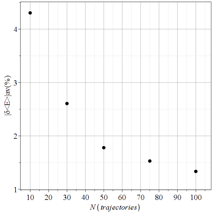
Figure 14: The mean absolute deviation (percent) between ensembles of chaotic trajectories in the case of full chaos, for $t\in[0,10^{5}]$ with a time step $\Delta t=50$ as a function of the trajectories in the ensemble. Even with a few trajectories we find an average value of energy very close to the theoretical one.

In fact, in a system where chaos is dominant one needs only a few trajectories in order to calculate with a satisfying accuracy the average values of quantum observable,s but at the cost of a large integration time. This can be seen in Fig. 14 where we plot the mean absolute deviations between the theoretical and numerical average energy in the multinodal wavefunction $\Psi=M(a\Psi_{10,3}+b\Psi_{4,5}+c\Psi_{7,8})$, which is dominated by chaotic trajectories, as a function of the number of trajectories in our sample. The trajectories are integrated up to $t=10^{5}$ and are sampled at every $\Delta t=50$. We see that even with a few chaotic trajectories we find quite accurate results. E.g. with only 50 trajectories we find an average error less than $2\%$. These results become more accurate if we extend the integration times.

On the other hand, the ordered trajectories are mainly concentrated near the maxima of the Born distribution. They cover only a small part of the configuration space and their long time shape is not common for all of them. Therefore a) they cannot be simulated neither by a few initial ordered trajectories according to Born’s rule and b) nor by many ordered trajectories that are not Born-distributed.

Our present work provides a better understanding of the role of order and chaos in BQM.

Appendix

The theoretical average value of the $\Psi=\Psi(m_{1},\sqrt{\omega_{1}}x)$ oscillator is

$$\langle p_{x}\rangle=-i\hbar\int_{-\infty}^{\infty}(\Psi^{*}\frac{\partial\Psi}{\partial x})dV$$ (18)

Since the operator $\hat{p}_{x}$ is $\hat{p}_{x}=-i\hbar\frac{\partial}{\partial x}$. In the case of a superposition of two terms $\Psi=a\Psi(m_{1},\sqrt{\omega_{1}}x)+b\Psi(m_{2},\sqrt{\omega_{1}}x)$ we set $\hbar=1$ and write

$$\Psi=\frac{a(\frac{\omega_{x}}{\pi})^{\frac{1}{4}}e^{\frac{-\omega_{x}x^{2}}{2}}H(m_{1},\sqrt{\omega_{x}}x)e^{-It(m_{1}+\frac{1}{2})\omega_{x}}}{\sqrt{2^{m_{1}}m_{1}!}}+\frac{b(\frac{\omega_{x}}{\pi})^{\frac{1}{4}}e^{\frac{-\omega_{x}x^{2}}{2}}H(m_{2},\sqrt{\omega_{x}}x)e^{-It(m_{2}+\frac{1}{2})\omega_{x}}}{\sqrt{2^{m_{2}}m_{2}!}}$$ (19)

The Hermite polynomials $H_{m}$ contain terms of degrees $m,m-2\dots$, i.e. of the same parity. The conjugate wavefunction $\Psi^{*}$ is found if we set $i\to-i$ in $\Psi$ since the Hermite polynomials are real.

After some algebra we find that

$$-(\Psi^{*}\frac{\partial\Psi}{\partial x_{i}})=\sum_{i}^{7}F_{i}.$$ (20)

where

$$F_{1}=\frac{i\omega_{x}^{\frac{3}{2}}H(m_{1},\sqrt{\omega_{x}}x)^{2}a^{2}x}{e^{\omega_{x}x^{2}}\sqrt{\pi}(a^{2}+b^{2})2^{m_{1}}m_{1}!}+\frac{i\omega_{x}^{\frac{3}{2}}H(m_{2},\sqrt{\omega_{x}}x)^{2}b^{2}x}{e^{\omega_{x}x^{2}}\sqrt{\pi}(a^{2}+b^{2})2^{m_{2}}m_{2}!}$$ (21)

$$F_{2}=\frac{i\omega_{x}^{\frac{3}{2}}\exp(it\omega_{x}m_{2})H(m_{2},\sqrt{\omega_{x}}xH(m_{1},\sqrt{\omega_{x}}x)2^{-1/2(m_{1}+m_{2})}abx}{e^{\omega_{x}x^{2}}\sqrt{\pi}\sqrt{m_{1}!}\sqrt{m_{2}!}(a^{2}+b^{2})\exp(i\omega_{x}m_{1}t)}$$ (22)

$$F_{3}=\frac{i\omega_{x}^{\frac{3}{2}}\exp(it\omega_{x}m_{1})H(m_{2},\sqrt{\omega_{x}}xH(m_{1},\sqrt{\omega_{x}}x)2^{-1/2(m_{1}+m_{2})}abx}{e^{\omega_{x}x^{2}}\sqrt{\pi}\sqrt{m_{1}!}\sqrt{m_{2}!}(a^{2}+b^{2})\exp(i\omega_{x}m_{2}t)}$$ (23)

$$F_{4}=-\frac{2i\omega_{x}H(m_{1}\sqrt{\omega_{x}}x)m_{1}H(m_{1}-1,\sqrt{\omega_{x}}x)a^{2}}{e^{\omega_{x}x^{2}}\sqrt{\pi}m_{1}!(a^{2}+b^{2})2^{m_{1}}}$$ (24)

$$F_{5}=-\frac{2i\omega_{x}H(m_{2}\sqrt{\omega_{x}}x)m_{2}H(m_{2}-1,\sqrt{\omega_{x}}x)b^{2}}{e^{\omega_{x}x^{2}}\sqrt{\pi}m_{2}!(a^{2}+b^{2})2^{m_{2}}}$$ (25)

$$F_{6}=-\frac{2i\omega_{x}H(m_{2}\sqrt{\omega_{x}}x)m_{1}H(m_{1}-1,\sqrt{\omega_{x}}x)ab2^{-1/2(m_{1}+m_{2})}\exp(i\omega_{x}tm_{2})}{e^{\omega_{x}x^{2}}\sqrt{\pi}m_{2}!(a^{2}+b^{2})2^{m_{2}}\exp(i\omega_{x}m_{1}t)}$$ (26)

$$F_{7}=-\frac{2i\omega_{x}H(m_{1}\sqrt{\omega_{x}}x)m_{2}H(m_{2}-1,\sqrt{\omega_{x}}x)ab2^{-1/2(m_{1}+m_{2})}\exp(i\omega_{x}m_{1}t)}{e^{\omega_{x}x^{2}}\sqrt{\pi}m_{2}!(a^{2}+b^{2})2^{m_{2}}\exp(i\omega_{x}m_{2}t)}$$ (27)

We note that in finding the derivative of $H_{m}(x)$ we used the formula $H^{\prime}_{m}(x)=2mH_{m-1}(x)$.

The integral from $-\infty$ to $\infty$ of $F_{1}$ is zero since both of its terms are odd functions. Similarly both $F_{4}$ and $F_{5}$ give zero integrals since they contain different Hermite polynomials which are orthogonal. Thus the only terms that may give a nonzero contribution in $\langle p_{x}\rangle$ are $F_{2},F_{3},F_{6}$ and $F_{7}$. The integrals of the functions $F_{2}$ and $F_{3}$ are of the form

$$\int_{-\infty}^{\infty}xe^{-x^{2}}H_{m}(x)H_{n}(x)dx=\pi^{1/2}2^{n-1}n!\delta_{m,n-1}+\pi^{1/2}2^{n}(n+1)!\delta_{m,n+1},$$ (28)

where $\delta_{r,s}$ stands for the Kronecker symbol ([27]). Therefore they are nonzero only if $m,n$ differ by 1. Finally, from $F_{6}$ and $F_{7}$ we find nonzero integrals only if $m_{2}=m_{1}-1$ or vice versa, i.e. the $m_{1}$ and $m_{2}$ should differ by 1 otherwise they give zero integrals.

If $\Psi$ is the sum of 3 terms $\Psi=a\Psi_{m_{1}}+b\Psi_{m_{2}}+c\Psi_{m_{3}}$ then we have also terms similar to $F_{1}-F_{7}$ between $\Psi_{m_{1}}$ and $\Psi_{m_{3}}$ and between $\Psi_{m_{2}}$ and $\Psi_{m_{3}}$. Thus in order to have an integral different from zero we must have $|m_{1}-m_{2}|=1$ or $|m_{1}-m_{3}|=1$ or $|m_{2}-m_{3}|=1$. If $\Psi$ depends both on $x$ and $y$,

$$\Psi=a\Psi_{m_{1}}(x)\Psi_{n_{1}}(y)+b\Psi_{m_{2}}(x)\Psi_{n_{2}}(y)+c\Psi_{m_{3}}(x)\Psi_{n_{3}}(y).$$ (29)

After the integration with respect to $x$ we have to integrate also with respect to $y$, as in Eq. 8. The only integrals $\int\Psi_{n}(y)\Psi_{n^{\prime}}(y)dy$ that are different from zero are those with $n=n^{\prime}$. Therefore in a term with $|m_{1}-m_{2}|=1$ we must also have $n_{1}=n_{2}$, in the term $|m_{1}-m_{3}|=1$ we must also have $n_{1}=n_{3}$, and in a term $|m_{2}-m_{3}|=1$ we must also have $n_{2}=n_{3}$.

Similar analytical expressions are found for $\langle p_{y}\rangle$ and $\langle L\rangle$. Regarding the position of the particles, the theoretical average value of $x$ in the case of two terms gives

$$\langle x\rangle=\int_{-\infty}^{\infty}\Psi^{*}x\Psi dx,$$ (30)

where $\Psi^{*}x\Psi$ contains terms of the form $xH_{m_{1}}^{2}(x),xH_{m_{2}}(x)^{2},$ and $xH_{m_{1}}(x)H_{m_{2}}(x)$. The integrals of the first two terms are zero. The integral of third term is different from zero only if $m_{1}$ and $m_{2}$ differ by 1. Similar results we find when $\Psi$ contains 3 terms in $x$.

Then if $\Psi$ depends also on $y$ we must integrate also with respect to $y$. This integration gives zero unless $|m_{1}-m_{2}|=1,n_{1}=n_{2}$ or $|m_{1}-m_{3}|=1,n_{1}=n_{3},$ or $|m_{2}-m_{3}|=1,n_{2}=n_{3}$.

Similarly, in calculating the theoretical average value of $y$ we have a result different from zero only if $|n_{1}-n_{2}|=1$ and $m_{1}=m_{2}$ or $|m_{1}-m_{3}|=1$ and $m_{2}=m_{3}$, or $|n_{2}-n_{3}|=1$ and $m_{2}=m_{3}$.

In the example of the single nodal point $\Psi=M(a\Psi_{0,0}+b\Psi_{1,0}+c\Psi_{1,1})$ we have $m_{1}=0,m_{2}=1,m_{3}=1$ and $n_{1}=0,n_{2}=0,n_{3}=1$. Therefore the x-integration for $\langle p_{x}\rangle$ gives two terms different from zero, those with $|m_{1}-m_{2}|=1$ and with $|m_{1}-m_{3}|=1$. The y-integration of the first term gives a non-zero term because $n_{1}=n_{2}=0$ while the integration of the second term gives zero, because $n_{2}\neq n_{3}$. The final result is given by Eq. 9. In a similar way we calculate $\langle p_{y}\rangle$ (Eq. 10), $\langle L\rangle$ (Eq. 11) $\langle x\rangle$ (Eq. 12) and $\langle y\rangle$ (Eq. 13).

In the example of many nodal points $\Psi=M(a\Psi_{0,2}+b\Psi_{3,4}+c\Psi_{5,7})$ (case 3.1) we have $m_{1}=0,m_{2}=3,m_{3}=5$ and $n_{1}=2,n_{2}=4,n_{3}=7$, therefore there are no terms with successive $m_{i},m_{j}$ and the values of $\langle p_{x}\rangle,\langle p_{y}\rangle$, $\langle L\rangle$, $\langle x\rangle$ and $\langle y\rangle$ are zero.

Similarly we have zero results in the case 3.2 when $\Psi=M(a\Psi_{10,3}+b\Psi_{4,5}+c\Psi_{7,8})$, while in the case $\Psi=M(a\Psi_{4,6}+b\Psi_{5,6}+c\Psi_{7,8})$ we have $\langle p_{x}\rangle$ different from zero, but $\langle p_{y}\rangle=0$.

References

- [1] D. Bohm, A suggested interpretation of the quantum theory in terms of ”hidden” variables. i, Phys. Rev. 85 (1952) 166.
- [2] D. Bohm, A suggested interpretation of the quantum theory in terms of ”hidden” variables. ii, Phys. Rev. 85 (1952) 180.
- [3] P. R. Holland, The quantum theory of motion: an account of the de Broglie-Bohm causal interpretation of quantum mechanics, Cambridge University Press, 1995.
- [4] E. Merzbacher, Quantum mechanics, John Wiley & Sons, 1998.
- [5] R. Shankar, Principles of quantum mechanics, Springer, 2012.
- [6] L. E. Ballentine, Quantum Mechanics: a Modern Development, World Scientific Publishing Company, 2014.
- [7] A. Valentini, Signal-locality, uncertainty, and the subquantum h-theorem. ii, Phys. Lett. A 158 (1991) 1.
- [8] A. Valentini, Signal-locality, uncertainty, and the subquantum h-theorem. i, Phys. Lett. A 156 (1991) 5.
- [9] M. Towler, N. Russell, A. Valentini, Time scales for dynamical relaxation to the Born rule, Proc. Roy. Soc. A 468 (2011) 990.
- [10] R. H. Parmenter, R. Valentine, Deterministic chaos and the causal interpretation of quantum mechanics, Phys. Lett. A 201 (1) (1995) 1.
- [11] S. Sengupta, P. Chattaraj, The quantum theory of motion and signatures of chaos in the quantum behaviour of a classically chaotic system, Phys. Lett. A 215 (1996) 119.
- [12] G. Iacomelli, M. Pettini, Regular and chaotic quantum motions, Phys. Lett. A 212 (1996) 29.
- [13] H. Frisk, Properties of the trajectories in Bohmian mechanics, Phys. Lett. A 227 (1997) 139.
- [14] H. Wu, D. Sprung, Quantum chaos in terms of bohm trajectories, Physics Letters A 261 (3-4) (1999) 150–157.
- [15] A. Makowski, P. Pepłowski, S. Dembiński, Chaotic causal trajectories: the role of the phase of stationary states, Phys. Lett. A 266 (4-6) (2000) 241–248.
- [16] A. J. Makowski, M. Frackowiak, The simplest non-trivial model of chaotic causal dynamics, Acta Phys. Polonica B 32.
- [17] A. J. Makowski, Forced dynamical systems derivable from bohmian mechanics, Acta Phys. Polonica B 33 (2) (2002) 583.
- [18] P. Falsaperla, G. Fonte, On the motion of a single particle near a nodal line in the de Broglie–Bohm interpretation of quantum mechanics, Phys. Lett. A 316 (2003) 382.
- [19] D. A. Wisniacki, E. R. Pujals, Motion of vortices implies chaos in Bohmian mechanics, Europhys. Lett. 71 (2005) 159.
- [20] D. Wisniacki, E. Pujals, F. Borondo, Vortex dynamics and their interactions in quantum trajectories, J. Phys. A 40 (2007) 14353.
- [21] F. Borondo, A. Luque, J. Villanueva, D. A. Wisniacki, A dynamical systems approach to Bohmian trajectories in a 2d harmonic oscillator, J. Phys. A 42 (2009) 495103.
- [22] A. Cesa, J. Martin, W. Struyve, Chaotic bohmian trajectories for stationary states, J. Phys. A 49 (2016) 395301.
- [23] A. C. Tzemos, G. Contopoulos, Unstable points, ergodicity and born’s rule in 2d bohmian systems, Entropy 25 (7) (2023) 1089.
- [24] A. C. Tzemos, G. Contopoulos, Chaos and ergodicity in an entangled two-qubit Bohmian system, Phys. Scr. 95 (2020) 065225.
- [25] A. Tzemos, G. Contopoulos, The role of chaotic and ordered trajectories in establishing Born’s rule, Phys. Scr. 96 (2021) 065209.
- [26] A. C. Tzemos, G. Contopoulos, Ergodicity and Born’s rule in an entangled two-qubit Bohmian system, Phys. Rev. E 102 (2020) 042205.
- [27] G. B. Arfken, H. J. Weber, F. E. Harris, Mathematical methods for physicists: a comprehensive guide, Academic press, 2011.