Time-efficient filtering of polarimetric data by checking physical realizability of experimental Mueller matrices
Abstract
Imaging Mueller polarimetry has already proved its potential for metrology, remote sensing and biomedicine. The real-time applications of this modality require both video rate image acquisition and fast data post-processing algorithms. First, one must check the physical realizability of the experimental Mueller matrices in order to filter out non-physical data, i.e. to test the positive semi-definiteness of the Hermitian coherency matrix calculated from the elements of the corresponding Mueller matrix pixel-wise. For this purpose, we compared the execution time for the calculations of i) eigenvalues, ii) Cholesky decomposition, iii) Sylvester’s criterion, and iv) coefficients of the characteristic polynomial of the Hermitian coherency matrix using two different approaches, all calculated for the experimental Mueller matrix images (600 pixels700 pixels) of mouse uterine cervix. The calculations were performed using C++ and Julia programming languages. Our results showed the superiority of the algorithm iv), in particular, the version based on the simplification via Pauli matrices, in terms of execution time for our dataset, over other algorithms. The sequential implementation of the latter algorithm on a single core already satisfies the requirements of real-time polarimetric imaging in various domains. This can be further amplified by the proposed parallelization (for example, we achieve a 5-fold speed up on 6 cores).
Mueller polarimetry, physical realizability of Mueller matrix, positive semi-definite Hermitian matrix, data filtering
1 Introduction
Mueller polarimetry (MP) is an optical technique that is used for the characterization of polarimetric properties of a sample for various applications such as metrology [1, 2, 3], remote sensing [4, 5], medical imaging [6, 7, 8, 9, 10], tissue engineering [11, 12], digital histology [13, 14, 15] material characterization [16, 17], food quality control [18], etc. By measuring the changes in polarization states of incident light upon interaction with a sample a MP system provides a set of 16 parameters that form a real-valued transfer matrix (so-called Mueller matrix (MM)) [19, 20, 21] of this sample. Each element of MM corresponds to a specific transformation of the input polarization state. Choosing an appropriate MM decomposition algorithm [22, 23, 24, 25, 26, 27] allows researchers to extract and analyze quantitatively the depolarization, retardance and diattenuation properties [19] of a sample which carry relevant metrological (or diagnostic) information.
The design and calibration of MM polarimeters are usually optimized in terms of minimizing the measurement errors [28, 29, 30, 31]. However, the presence of the residual systematic and random experimental errors may lead to nonphysical measurement results at certain measurement wavelengths or/and at certain image pixels, i. e. produce a particular real-valued matrix that does not obey the condition of physical realizability for MM (see Sec.2.1). It is worth to mention that a necessary and sufficient condition for the physical realizability of Mueller matrix requires the corresponding Hermitian coherency matrix (HCM) [19] to be a positive semi-definite matrix [23, 32]. Thus, checking this condition for all acquired MMs represents a must step of the polarimetric data post-processing for filtering out nonphysical data.
In particular, the imaging MM polarimeters operating in either real [11, 6, 7] or reciprocal [3] space produce a significant amount of polarimetric data at each single measurement, because the total number of image pixels is quite large (the resolution of CCD cameras is typically several hundreds of thousands pixels or more). Consequently, for the real-time imaging applications with a tight time budget it is important to find the most time-efficient algorithm for checking pixel-wise whether a HCM is a positive semi-definite one.
The paper is organized as follows: in the next section we describe the basics of Stokes-Mueller formalism and the MM images of mouse uterine cervix taken with the custom-built MM polarimetric system and used in our studies. Four different approaches for testing the physical realizability of the measured MMs, namely, the calculations of i) eigenvalues, ii) Cholesky decomposition, iii) Sylvester’s criterion , and iv) coefficients of the characteristic polynomial of the corresponding HCM and the comparison of these algorithms in terms of the execution time and accuracy are presented and discussed in the third section of the paper. The last section summarizes our results and discuss the perspectives of potential applications.
2 Materials and Methods
2.1 Stokes-Mueller formalism
In this section we briefly recall the theoretical framework for the description of fully or partially polarized light.
Apart from light intensity and color the polarization of light reflects its vectorial nature. Let us consider the propagation of a plane polarized monochromatic electromagnetic (EM) wave through an infinite isotropic medium. By selecting a Cartesian coordinate system with axis parallel to the direction of wave propagation (, where is a wave number) the oscillation of the electric field (EF) vector at the point is confined to the plane - orthogonal to axis and is described by a superposition of two independent harmonic oscillators [19]
| (1) |
where and are the constant amplitudes, is the angular frequency, is the wavenumber, and are the arbitrary constant phases, and the subscripts and refer to the field components in the - and -directions, respectively. Equations (1) can be re-written as
| (2) |
where is the phase shift between the orthogonal transverse components of EF vector of a plane EM wave. Equation (2) describes a polarization ellipse that represents the trajectory of a tip of oscillating EF vector of polarized light. However, the direct observation of the polarization ellipse is impossible, because optical EF vector traces out the locus of points described by (2) in a time interval of order s.
For partially or completely depolarized light the motion of EF vector is disordered in - plane and can be described by its probability distribution only. We cannot observe the amplitude of optical EF, but we can observe and measure the intensity of light. For linear optical systems the measured intensity is obtained by averaging the square of EF amplitude and represents the second moments (quadratic quantities) of the EF distribution.
We denote the intensities related to the components of the EF vector parallel to and axes as , , respectively. The angle brackets indicate temporal, spatial and spectral averaging, which depends on both sample and measurement conditions. We define four observable Stokes parameters as
| (3) |
The parameter is the total intensity of light, represents the difference in the light intensities measured after a linear polarizer with optical axis aligned parallel with either or axes. The parameter is equivalent to the parameter , but the intensities are measured after a linear polarizer with optical axis aligned at either or , respectively, within the plane orthogonal to the direction of light beam propagation. The parameter represents the difference between the intensities transmitted by either left or right circular polarizer.
We define the Stokes vector as The degree of polarization of any Stokes vector is defined as
| (4) |
where parameter varies between 0, for totally depolarized light, and 1, for totally polarized light. Upon interaction with a sample the Stokes vector of incident light undergoes a linear transformation, described by a real-valued matrix , which is called a Mueller matrix (MM) [19] of a sample.
| (5) |
It is obvious that physically realizable MM should transform any Stokes vector of incident light beam into a Stokes vector of output light beam with the degree of polarization less than or equal to 1. An Hermitian coherency matrix associated with matrix is defined as in [21]:
| (6) |
where is the Kronecker product of matrices and is an extended set of Pauli matrices [33]:
It was demonstrated by Cloude [23, 32] that a real-valued matrix represents a physically realizable MM if and only if the associated HCM calculated in (6) is a positive semi-definite matrix. Due to the presence of measurement systematic errors and noise, this condition may not always be satisfied for the experimental polarimetric data. Thus, these data must undergo a physical realizability filtering before further data post-processing.
2.2 Mueller matrix images of mouse uterine cervix
Imaging Mueller polarimetry has proven its potential for various biomedical applications by helping the clinicians to make better decisions about patient diagnosis and treatment [9, 34, 35]. The translation of this modality into clinical practice requires video rate image acquisition and the development and implementation of fast polarimetric data post-processing algorithms. As was mentioned above the pixel-wise test of physical realizability of MM images is a first step of polarimetric data post-processing.
In our studies we used the experimental Mueller matrix images (600 pixels 700 pixels) of thin section (nominal thickness 50 ) of mouse uterine cervix (Fig.1). The research protocols were reviewed and approved by the Florida International University (registration number: IACUC-20-014).
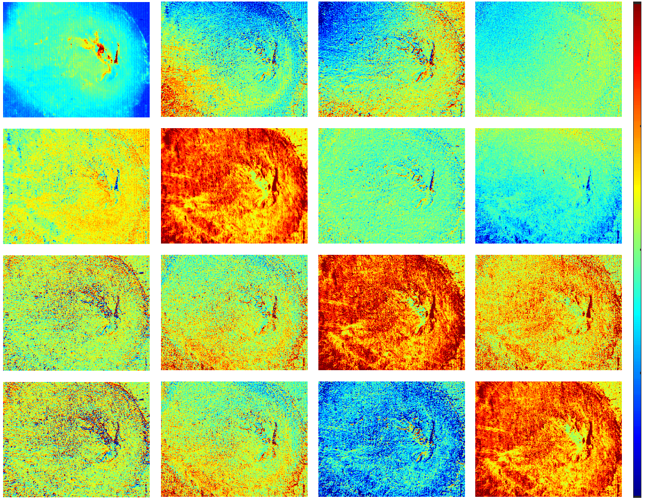
These images were acquired with the custom-built imaging Mueller polarimetric system described in [36]. The modulation of incident light polarization and analysis of the detected signal was performed with the rotating quarter-wave plates and fixed polarizers inserted into both illumination and detection arm of the instrument. A 550-nm LED (Thorlabs, Newton, New Jersey) was used as a light source, a sCMOS camera (pco.edge by PCO, Kelheim, Germany) was used as a detector for the image registration. The system calibration was done with the eigenvalue calibration method described by Compain [31]. The experimental errors on the elements of measured Mueller matrix of air (it should be a unity matrix) were below 1%. The complete description of the experimental setup can be found in [36].
During data post-processing step the check on physical realizability of each matrix from the dataset containing 420000 () matrices has to be performed first. Given the massive amount of polarimetric data to be tested one needs to find the most time-efficient algorithm for checking the physical realizability of large dataset of MMs (i. e. positive semi-definiteness of the corresponding HCMs).
3 Tests on positive semi-definiteness of HCM
3.1 Algorithms
Definition: Hermitian matrix is positive semi-definite (or definite) if (or ) for all .
We have tested four different approaches for checking the positive semi-definiteness (or positive definiteness) of HCM by calculating:
-
•
eigenvalues of HCM,
-
•
Cholesky decomposition of HCM,
-
•
Sylvester’s criterion for HCM,
-
•
coefficients of HCM characteristic polynomial.
It is worth considering both the pros and cons of each algorithm for filtering out nonphysical polarimetric data.
3.1.1 HCM eigenvalues
Nowadays, the most common test for the physical realizability of a MM relies on the calculation of eigenvalues of the corresponding HCM [23, 37, 32]. All eigenvalues are nonnegative for a positive semi-definite matrix. Moreover, if MM of a sample is partially or completely depolarizing, the corresponding HCM must be a positive definite matrix. The latter comment is particularly relevant for almost all types of biological tissue because of strong light scattering within biotissue leading to the significant depolarization of detected scattered light [38].
This method is widely spread, because one may not only filter out nonphysical data but also use a vector measure of depolarization based on the three smallest nonnegative eigenvalues as of the physically realizable MM. It was shown that such a metric may increase the polarimetric image contrast for certain classes of samples [39, 26, 40]. However, for a wide class of samples, it is not necessary to know the exact eigenvalues of HCM, when one needs to evaluate the sign of eigenvalues only.
3.1.2 Cholesky decomposition of HCM
A decomposition of a Hermitian positive definite matrix into the product of a lower triangular matrix and its conjugate transpose matrix is called Cholesky decomposition: , and Cholesky decomposition is unique for such matrix [41]. To test whether a Hermitian matrix is positively definite using Cholesky decomposition, one needs to check whether the signs of all diagonal elements of the lower triangular matrix are positive. The fact that Cholesky decomposition may address the HCM positive definiteness only is not very restrictive for medical applications of MP, because, in general, biological tissue are highly depolarizing media and the corresponding HCMs are positive definite.
3.1.3 Sylvester’s criterion
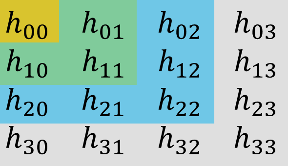
Sylvester’s criterion of positive definiteness of an arbitrary Hermitian matrix states that this matrix is positive definite if and only if all its leading principal minors are positive [42, 43, 32]. In case of a HCM it means that all following matrices have a positive determinant:
-
•
upper left sub-matrix of HCM,
-
•
upper left sub-matrix of HCM,
-
•
upper left sub-matrix of HCM,
-
•
HCM itself.
The choice of corresponding elements of HCM for the calculations of leading principal minors is illustrated in Fig.2.
In the actual implementation, we applied (in advance) Maple’s command simplify to each of the determinant expressions to decrease the computing time.
3.1.4 Coefficients of HCM characteristic polynomial
The characteristic polynomial (CP) of arbitrary matrix is defined as function , where represents the identity matrix [44] (here we used “” instead of the standard “” in the definition of CP so that it will be easier to state the criterion). An arbitrary matrix with real eigenvalues is positive semi-definite if and only if all coefficients of its characteristic polynomial are nonnegative. This is true by applying Descartes’ rule of signs [45] to and using the equivalence between positive semi-definiteness and non-negativity of the eigenvalues.
It turns out that the actual presentation of the formulas for the coefficients of can affect the computing time. In what follows, we use two versions for the presentation of the coefficients:
-
•
formulas separately simplified in Maple using command simplify
-
•
formulas obtained using Pauli matrices [33] as described below.
The coefficients of the CP of are the elementary symmetric polynomials of its eigenvalues . We could find the values of these polynomials using the Newton identities [46, p. 23] if we knew the values of the power sums for . These power sums, in turn, are exactly the traces . For computing these traces, we will use the following observations:
-
•
Any power of is again a linear combination of the form (6);
-
•
if and only if , and it is equal to otherwise.
The latter property immediately gives us a simple formula . For the second degree, we observe that the only way to obtain as a product of two Pauli matrices is to take a square. This implies that
Using similar but much more tedious combinatorial considerations, we have obtained formulas for and , presented in the Appendix.
3.2 Comparison of the results: execution time and accuracy
All algorithms described in Sec. 3.1 were tested on the experimental Mueller matrix data described in Sec. 2.1. The results of the comparison in terms of the execution time depending the number of used CPU cores are shown in Tab. 1. The code was written in C++, and the experiments were performed on a Mac computer with CPU 3.1 GHz 6-Core Intel Core i5 and 16 GB. For the eigenvalue computation and Choletsky decomposition we used the numerical linear algebra library Eigen [47] (version 3.4.0). The C++ compiler was Clang 13.1.6, and the Mac OS version was 12.3. The runtimes were averaged over 20 runs; the standard deviation was or lower. The implementation is available here: https://github.com/pogudingleb/mueller_matrices.
Section 3.1 checking whether 420,000 Mueller matrices are physically realizable
| 1 | 2 | 3 | 4 | 5 | 6 | |
|---|---|---|---|---|---|---|
| Eigen’s self-adjoint eigensolver | 561.3 | 289.1 | 194.3 | 145.5 | 119.2 | 99.5 |
| Eigen’s Cholesky decomposition | 49.6 | 25.5 | 17.1 | 13.0 | 10.6 | 8.8 |
| Sylvester’s criterion | 34.6 | 17.7 | 11.9 | 9.0 | 7.4 | 6.3 |
| Coefficients of CP (via Maple simplify) | 26.8 | 13.5 | 9.1 | 6.9 | 5.6 | 4.7 |
| Coefficients of CP (simplification via Pauli matrices) | 13.1 | 6.6 | 4.5 | 3.5 | 2.9 | 2.6 |
The number of filtered out nonphysical matrices is 868 and constitutes approximately of the total number of matrices for all tested algorithms, thus, proving the good quality of our experimental polarimetric data. In addition, all nonphysical data were found at the same image pixels by all algorithms. So, all the algorithms were numerically stable enough for the considered data.
Our computational experiments confirm that the method of calculations of HCM eigenvalues for checking positive definiteness (semi-definiteness) of HCM is orders of magnitude slower and more memory demanding compared to other three methods.
We achieve additional speed-up by parallelization. Indeed, the matrix for each pixel can be processed independently of the other pixels. On our 6-core environment we achieved a run-time speed-up of approximately 5.5 times over the sequential computation. This is more than enough for the processing of the matrices to be used in real-time.
For comparison, we also ran this in Julia version 1.10.0 in CentOS Linux 7, on Intel(R) Xeon(R) CPU E5-2680 v2 @ 2.80GHz, with 20 cores, and found out that the relative placement of the algorithms in terms of runtime is the same as that of our C++ code. Our Julia implementations of the algorithms via Sylvester’s criterion and via coefficients of the CP are also sufficiently fast to be used in real time. The detailed results are reported here: https://github.com/pogudingleb/mueller_matrices/blob/main/src_julia/julia_code.out.
4 Conclusion
Our results on checking pixel-wise physical realizability of the experimental Mueller matrix images of mouse uterine cervix demonstrated the superiority of two algorithms (Sylvester’s criterion and calculations of the coefficients of the characteristic polynomial of HCM) for our dataset, in terms of execution time compared to other considered algorithms, whereas keeping the same accuracy. It is quite logical that the filtering method based on the calculations of HCM eigenvalues may not be optimal because we generate the redundant data, i. e. the absolute values of the eigenvalues of HCM, that are not used for MM filtering.
Another explanation for the observed performance gap is related to the fact that general-purpose linear algebra software is often not optimized for the matrices of small dimensions (e. g. ), which we consider in this paper.
Our findings are important for many applications of MP that generate significant amount of polarimetric data and require both real-time data acquisition and fast data post-processing algorithms, in particular, for imaging MP used for i) metrology in semi-conductor industry, and ii) in vivo medical diagnosis and surgery guidance in clinical settings.
Appendix
In this appendix, we will provide explicit formulas for and , which we obtained through combinatorial considerations with Pauli matrices. Let denote the lower-right -submatrix of .
We start with . We have
For , we will introduce some intermediate variables. Let for , and define
Then, for , we set
and define
We also define
Then the final formula will be:
The automatic verification of the formulas performed using Maple can be found in the repository111https://github.com/pogudingleb/mueller_matrices/blob/main/formula.mpl.
Acknowledgments
We thank Georgy Scholten for fruitful discussions and valuable advice. We also thank the Courant Institute of Mathematical Sciences for its computational resources. None of the authors declare any conflict of interest.
Data availability
The experimental Mueller matrix data and codes for all algorithms used in the current study are available in the repository: https://github.com/pogudingleb/mueller_matrices.
References
References
- [1] T. Novikova and P. Bulkin. Inverse problem of Mueller polarimetry for metrological applications. J. Inverse Ill-Posed Probl., 29:759–774, 2021.
- [2] S. S. Liu, W. Du, X. Chen, H. Jiang, and C. Zhang. Mueller matrix imaging ellipsometry for nanostructure metrology. Opt. Express, 23(13):17316–17329, 2015.
- [3] C. Fallet, T. Novikova, M. Foldyna, S. Manhas, B. Haj Ibrahim, A. De Martino, C. Vannuffel, and C. Constancias. Overlay measurements by Mueller polarimetry in back focal plane. J. Micro/Nanolith. MEMS MOEMS, 10(3):033017, 2011.
- [4] G. W. Kattawar and M. J. Raković. Virtues of Mueller matrix imaging for underwater target detection. Appl. Opt., 38:6431–6438, 1999.
- [5] J. Li, J. Wei, H. Liu, J. Wan, T. Huang, H. Wang, R. Liao, M. Yan, and H. Ma. Polarization fingerprint for microalgae classification. Opt. Lasers Eng., 166:107567, 2023.
- [6] H. R. Lee, I. Saytashev, V. N. Du Le, M. Mahendroo, J. C. Ramella-Roman, and T. Novikova. Mueller matrix imaging for collagen scoring in mice model of pregnancy. Sci. Rep., 11(1):15621, 2021.
- [7] T. Novikova, A. Pierangelo, P. Schucht, I. Meglinski, O. Rodriguez-Nunez, and H. R. Lee. Mueller polarimetry of brain tissues. In Polarized light in Biomedical Imaging and Sensing, page 205–230. J. C. Ramella-Roman and T. Novikova (Eds), Springer, Sham, 2022.
- [8] A. Vitkin, N. Ghosh, and A. De Martino. Tissue polarimetry. In Photonics: Biomedical Photonics Spectroscopy, and Microscopy. D. L. Andrews (Ed.), Wiley & Sons, Inc., 2015.
- [9] A. Pierangelo, S. Manhas, A. Benali, M. R. Antonelli, T. Novikova, P. Validire, B. Gayet, and A. De Martino. Use of Mueller polarimetric imaging for the staging of human colon cancer. Proc. SPIE, Optical Biopsy IX, 7895:65–72, 2011.
- [10] J. Bonaventura, K. Morara, R. Carlson, C. Comrie, N. Daigle, E. Hutchinson, and T. W. Sawyer. Backscattering Mueller matrix polarimetry on whole brain specimens shows promise for minimally invasive mapping of microstructural orientation features. Front. Photon., 3, 2022.
- [11] D. Ivanov, A. Hoeppel, T. Weigel, R. Ossikovski, S. Dembski, and T. Novikova. Assessment of the impact of nanowarming on microstructure of cryopreserved fibroblast-containing 3D tissue models using Mueller polarimetry. Photonics, 10(10):1129, 2023.
- [12] D. Fricke, A. Becker, L. Jütte, M. Bode, D. de Cassan, M. Wollweber, B. Glasmacher, and B. Roth. Mueller matrix measurement of electrospun fiber scaffolds for tissue engineering. Polymers, 11:2062, 2019.
- [13] H. R. Lee, C. Lotz, F. Kai Groeber-Becker, S. Dembski, and T. Novikova. Digital histology with Mueller polarimetry and FastDBSCAN. Appl. Opt., 61(32):9616–9624, 2022.
- [14] L. Xia, Y. Yao, Dong Y., M. Wang, H. Ma, and L. Ma. Mueller polarimetric microscopic images analysis based classification of breast cancer cells. Opt. Commun., 475:126194, 2020.
- [15] V. A. Ushenko, B. T. Hogan, A. Dubolazov, G. Piavchenko, S. I. Kuznetsov, A. G. Ushenko, Y. O. Ushenko, M. Gorsky, A. Bykov, and I. Meglinski. 3D Mueller matrix mapping of layered distributions of depolarisation degree for analysis of prostate adenoma and carcinoma diffuse tissues. Sci. Rep., 11:5162, 2021.
- [16] S. A. Hall, M.-A. Hoyle, J. S. Post, and D. K. Hore. Combined Stokes vector and Mueller matrix polarimetry for materials characterization. Anal. Chem., 85(15):7613–7619, 2013.
- [17] O. Arteaga and B. Kahr. Mueller matrix polarimetry of bianisotropic materials. J. Opt. Soc. Am. B, 36(8):F72–F83, Aug 2019.
- [18] D. N. Ignatenko, A. V. Shkirin, Y. P. Lobachevsky, and S. V. Gudkov. Applications of Mueller matrix polarimetry to biological and agricultural diagnostics: A review. Appl. Sci., 12(10):5258, 2022.
- [19] D. H. Goldstein. Polarized light. (3rd ed. CRC Press), 2010.
- [20] R. M. A. Azzam. Propagation of partially polarized light through anisotropic media with or without depolarization: A differential 44 matrix calculus. J. Opt. Soc. Am., 68(12):1756 – 1767, 1978.
- [21] J. J. Gil-Perez and R. Ossikovski. Polarized Light and the Mueller Matrix Approach. (2nd Ed. CRC Press), Boca Raton, FL, USA, 2022.
- [22] S. Y. Lu and R. A. Chipman. Interpretation of Mueller matrices based on polar decomposition. J. Opt. Soc. Am.A, 13:1106–1113, 1996.
- [23] S. R. Cloude. Group theory and polarisation algebra. Optik, 75:26–36, 1986.
- [24] P. Li, H. R. Lee, S. Chandel, C. Lotz, F. Kai Groeber-Becker, S. Dembski, R. Ossikovski, H. Ma, and T. Novikova. Analysis of tissue microstructure with Mueller microscopy: logarithmic decomposition and Monte Carlo modeling. J. Biomed. Opt., 25(1):015002, 2020.
- [25] W. Sheng, W. Li, J. Qi, T. Liu, H. He, Y. Dong, S. Liu, J. Wu, D. S. Elson, and H. Ma. Quantitative analysis of 4 × 4 Mueller matrix transformation parameters for biomedical imaging. Photonics, 6(1):34, 2019.
- [26] J. J. Gil, I. San José, M. Canabal-Carbia, I. Estévez, E. González-Arnay, J. Luque, T. Garnatje, J. Campos, and A. Lizana. Polarimetric images of biological tissues based on the arrow decomposition of Mueller matrices. Photonics, 10(6):669, 2023.
- [27] N. Ghosh, M. F. Wood, S. H. Li, R. D. Weisel, B. C. Wilson, R. K. Li, and I. A. Vitkin. Mueller matrix decomposition for polarized light assessment of biological tissues. J Biophotonics, 2(3):145–56, 2009.
- [28] J. S. Tyo. Design of optimal polarimeters: maximization of signal-to-noise ratio and minimization of systematic error. Appl. Opt., 41(4):619–630, 2002.
- [29] A. De Martino, E. Garcia-Caurel, B. Laude, and B. Drévillon. General methods for optimized design and calibration of Mueller polarimeters. Thin Solid Films, 455:112–119, 2004.
- [30] N. C. Bruce and I. Montes-González. The effect of experimental errors on optimized polarimeters. Proc. SPIE, Polarization Science and Remote Sensing XI, 12690:141–147, 2023.
- [31] E. Compain, S. Poirier, and B. Drevillon. General and self-consistent method for the calibration of polarization modulators, polarimeters, and Mueller-matrix ellipsometers. Appl. Opt., 38:3490–3502, 1999.
- [32] S. R. Cloude. Conditions for the physical realisability of matrix operators in polarimetry. Proc. SPIE, 116:177–185, 1989.
- [33] R. Feynman, R. Leighton, M. Sands, M. Linzee Sands, and M. A. Gottlieb. The Feynman Lectures on Physics. volume III, chapter 11. Pearson/Addison-Wesley, 2006.
- [34] J. Vizet, J. Rehbinder, S. Deby, S. Roussel, A. Nazac, S. Soufan, C. Genestie, C. Haie-Meder, H. Fernandez, F. Moreau, and A. Pierangelo. In vivo imaging of uterine cervix with a Mueller polarimetric colposcope. Sci. Rep., 7:2471, 2017.
- [35] J. Qi and D. S. Elson. Mueller polarimetric imaging for surgical and diagnostic applications: a review. J. Biophotonics, 10(8):950–982, 2017.
- [36] T. Novikova and J. C. Ramella-Roman. Is a complete Mueller matrix necessary in biomedical imaging? Opt. Lett., 47(21):5549–5552, 2022.
- [37] J. J. Gil. On optimal filtering of measured Mueller matrices. Appl. Opt., 55(20):5449–5455, 2016.
- [38] V. Tuchin. Tissue Optics : Light Scattering Methods and Instruments for Medical Diagnosis. (2nd Ed. SPIE Press), 2007.
- [39] X. Li, L. Zhang, P. Qi, Z. Zhu, J. Xu, T. Liu, J. Zhai, and H. Hu. Are indices of polarimetric purity excellent metrics for object identification in scattering media? Remote Sens., 14(17):4148, 2022.
- [40] C. J. R. Sheppard, A. Bendandi, A. Le Gratiet, and A. Diaspro. Characterization of the Mueller matrix: Purity space and reflectance imaging. Photonics, 9(2):88, 2022.
- [41] C. N. Haddad. Cholesky factorization. In Encyclopedia of Optimization, pages 374–377. C. A. Floudas, P. M. Pardalos, (Eds) Springer US, Boston, MA, 2009.
- [42] J. J. Gil. Characteristic properties of Mueller matrices. J. Opt. Soc. Am. A, 17(2):328–334, 2000.
- [43] G. T. Gilbert. Positive definite matrices and Sylvester’s criterion. American Math. Mon., 98(1):44–46, 1991.
- [44] B. P. Brooks. The coefficients of the characteristic polynomial in terms of the eigenvalues and the elements of an matrix. Appl. Math. Lett., 19(6):511–515, 2006.
- [45] X. Wang. A simple proof of Descartes’s rule of signs. The American Mathematical Monthly, 111(6):525–525, 2004.
- [46] I. G. Macdonald. Symmetric functions and Hall polynomials. Oxford Science Publications, 1995.
- [47] G. Guennebaud, B. Jacob, et al. Eigen v3. http://eigen.tuxfamily.org, 2010.