Extended Kalman filter—Koopman operator for tractable stochastic optimal control

Abstract

It has been more than seven decades since the introduction of the theory of dual control [1]. Although it has provided rich insights to the fields of control, estimation, and system identification, dual control is generally computationally prohibitive. In recent years, however, the use of Koopman operator theory for control applications has been emerging. The paper presents a new reformulation of the stochastic optimal control problem that, employing the Koopman operator, yields a standard LQR problem with the dual control as its solution. We conclude the paper with a numerical example that demonstrates the effectiveness of the proposed approach, compared to certainty equivalence control, when applied to systems with varying observability.

I Introduction

Deterministic control theory carries the implicit assumption of complete access to the states, a condition not met in many applications of interest [2]. This renders the validity of the implemented control algorithms questionable. Instead, if the lack/partial access to the states is to be acknowledged, the resulting problem falls within the realm of stochastic optimal control (SOC) [3], which is not only concerned with controlling/regulating the state (as in deterministic control) but control/regulate all the involved uncertainties as well. Unfortunately, SOC is hindered in practice by its computational complexity, limiting its benefits to the conceptual level (exploration vs exploitation, stochastic tubes, persistence of excitation) in guiding control/observer design [4], experiment design and system identification [5].

SOC leads to two key qualitative outcomes: caution and probing [4], forming the two properties of a dual controller. Caution is the control behavior that limits the effects of uncertainty on safety and performance. Probing, often in conflict with caution, reflects the active information gathering that seeks regulating the system’s uncertainty. Caution, to some extent, is manifested through constraint tightening in tube-based MPC or satisfying constraint instances in scenario- or sample-based methods [6]. However, probing is absent in the control of unconstrained stochastic linear systems with quadratic costs, as the state error covariance is not a function of the control input. For linear systems with unknown parameters, probing can be achieved through the injection of a random signal [5] that persistently excites the system. In general nonlinear systems, however, system uncertainties depend on the control input, and random noise injection is often insufficient. Instead, effective probing requires reasoning about the future measurement program [3], leading to a computationally prohibitive formulation.

We target solving a dual control problem of a general differentiable nonlinear system using a quadratic cost, the typical form in most regulation/tracking problems. We choose the extended Kalman filter (eKF) as the approximator of the state uncertainty propagation. The eKF is simple and wide-spread in navigation [7], robotics [8], computer vision [9], power systems [10] and many other fields. Furthermore, the finite-dimensional approximation of the state uncertainty offered by the eKF (mean vector and covariance matrix) is appealing from the computational perspective. In particular, we show that a quadratic cost function can be written in terms of the eKF state.

The intractability of SOC persists even when employing the eKF approximation of uncertainty, thus, ruling out conventional solution algorithms. Dynamic Programming is “very unscalable” with state dimension and therefore restrictive. Nonlinear MPC, over the stochastic dynamics (eKF states), requires non-convex programming procedures which can be computationally demanding and/or ill-suited for online computation. These two options have in common that their problem formulations can be straightforward, while the challenge is in finding the solution. In contrast, our approach, which leverages the Koopman operator, switches the challenge from solution finding to problem formulation. That is, upon a successful identification of a suitable basis dictionary for the Koopman operator to represent the original system, the solution is a straightforward LQR problem. This discussion on where the challenge/art is located, in the formulation or the solution, resembles the discussion in [11, p. 10], explaining the dichotomy between convex and non-convex programs.

We reformulate the SOC problem such that it is amenable to the application of the Koopman operator theory. We discuss the structure of the new formulation, and list the assumptions required for the continuity, bilinearity, robust stability of the resulting new dynamics. The paper with a numerical example of a system from an important class in the system identification literature [12].

II Problem Formulation

Consider the dynamic system

$$x_{k+1} =f(x_{k},u_{k})+w_{k},$$ (1a)

$$y_{k} =h(x_{k},u_{k})+v_{k},$$ (1b)

where $x_{k}\in\mathbb{R}^{r_{x}}$ is the state, $u_{k}\in\mathbb{R}^{r_{u}}$ the control input and $y_{k}\in\mathbb{R}^{r_{y}}$ the measured output. The functions $f$ and $h$ are differentiable almost everywhere in their first arguments. The exogenous disturbances $w_{k}\in\mathbb{R}^{r_{x}}$, $v_{k}\in\mathbb{R}^{r_{y}}$, is each independent and identically distributed according to a density function. They are independent from each other and from $x_{0}$, for all $k$, and have zero means, and covariances $\Sigma_{w}$ and $\Sigma_{v}$, respectively. The initial state $x_{0}$ has a bounded mean $x_{0\mid-1}$, bounded covariance $\textbf{Cov}(x_{0})=\Sigma_{0\mid-1}$, and a density $p_{0}$.

Assumption 1.

(i) $\Sigma_{v},\,\Sigma_{w}$ and $\Sigma_{0\mid-1}$ are $\succ 0$, and bounded. (ii) $w_{k}\in W\subset\mathbb{R}^{r_{x}}$, $u_{k}\in\mathbb{U}\subset\mathbb{R}^{r_{u}}$, such that $W$ and $\mathbb{U}$ yield a compact set $\mathbb{X}$ invariant under (1a), starting from $x_{0}\in\mathbb{X}$. (iii) the sequence of events is as follows: at time $k$, $u_{k}$ is applied, then $y_{k}$ becomes available.

The goal in this paper is to design a feedback control policy that minimizes the following quadratic, finite-horizon cost $J^{N}(X_{0},U_{N-1})$ (we suppress its arguments for compactness)

$$J^{N}=\frac{1}{N}\cdot\mathbb{E\,}\Bigg{\{}x_{N}^{\top}Qx_{N}+\sum_{k=0}^{N-1}x_{k}^{\top}Qx_{k}+u_{k}^{\top}Ru_{k}\Bigg{\}},$$ (2)

where $U_{N-1}=\{u_{0},\ldots,u_{N-1}\}$, the tuple $X_{0}=(x_{0\mid-1},\Sigma_{0\mid-1})$, and $Q\succeq 0$ and $R\succ 0$ are symmetric matrices. The expectation is over the probability space $\mathbb{P}_{0}$, characterizing the random variables $(x_{0},V_{N-1},W_{N-1})$, where $V_{N-1}=\{v_{0},\ldots,v_{N-1}\}$ and $W_{N-1}=\{w_{0},\ldots,w_{N-1}\}$, and the corresponding product Borel $\sigma$-field.

The control input is admissible when it is a causal law. It is restricted to be a function of the accessible data up to the time-step of evaluating this law. That is, according to the $3$rd point of Assumption 1, $u_{k}=u_{k}(Z_{k-1})$, where $Z_{k-1}=\{p_{0},Y_{k-1},U_{k-1}\}$ stores all the past and accessible information up to time-$k$, prior to implementing $u_{k}$. Here $Y_{k-1}=\{y_{0},\ldots,y_{k-1}\}$. For consistency, we denote the prior information by $Z_{-1}=\{p_{0}\}$.

III Methodology

We first show that the cost (2) can be re-written in terms of the first two moments of $x_{k}$.

III-A Equivalent description to the cost

Lemma 1.

The term $\mathbb{E\,}x_{k}^{\top}Qx_{k}$ can be equivalently expressed by

$$\mathbb{E\,}\left\{x_{k}^{\top}Qx_{k}\right\}=\textit{tr}(Q\Sigma_{k\mid k-1})+\mathbb{E\,}\left\{x_{k\mid k-1}^{\top}Qx_{k\mid k-1}\right\}.$$

Here expectation on the left-hand-side can be expressed in its integral form as $\mathbb{E\,}\{x_{k}^{\top}Qx_{k}\}=\int x_{k}^{\top}Qx_{k}p(x_{k})dx_{k}$ with respect to the density function $p(x_{k})$. The other expectation can be stated as

$$\mathbb{E\,}\left\{x_{k\mid k-1}^{\top}Qx_{k\mid k-1}\right\}=\int x_{k\mid k-1}^{\top}Qx_{k\mid k-1}p(Y_{k-1})dY_{k-1}.$$

Here the first two conditional central moments are

$$x_{k\mid k-1} =\mathbb{E\,}\left\{x_{k}\mid Z_{k-1}\right\},$$ (3)

$$\Sigma_{k\mid k-1} =\mathbb{E\,}\left\{[x_{k}-x_{k\mid k-1}][x_{k}-x_{k\mid k-1}]^{\top}\mid Z_{k-1}\right\}.$$

Proof.

This lemma is a direct consequence of the law of total expectation (smoothing theorem) [14, p. 348], if we condition each additive term in (2) on its corresponding (with respecting causality) $Z_{k-1}$. That is,

$$\hskip-14.22636pt\mathbb{E\,}\left\{x_{k}^{\top}Qx_{k}\right\}=\int x_{k}^{\top}Qx_{k}p(x_{k})dx_{k},$$

$$=^{\star}\int\int x_{k}^{\top}Qx_{k}p(x_{k},Y_{k-1})d\,Y_{k-1}dx_{k},$$

$$=\int\left(\int x_{k}^{\top}Qx_{k}p(x_{k}\mid Y_{k-1})dx_{k}\right)p(Y_{k-1})dY_{k-1},$$

$$=\mathbb{E\,}\left\{\mathbb{E\,}\left\{x_{k}^{\top}Qx_{k}\mid Z_{k-1}\right\}\right\},$$ (4)

where the equality with an asterisk follows from evaluating $p(x_{k})$ through marginalizing the joint $p(x_{k},Y_{k-1})$.

For the inner conditional expectation in (4), the state $x_{k}$ can be decomposed into $x_{k}=x_{k\mid k-1}+\tilde{x}_{k}$, where $\tilde{x}_{k}$ is the prediction error. The quadratic term $x_{k}^{\top}Qx_{k}=(x_{k\mid k-1}+\tilde{x}_{k})^{\top}Q(\hat{x}_{k\mid k-1}+\tilde{x}_{k})$, under the conditional expectation $\mathbb{E\,}\left\{\cdot\mid Z_{k-1}\right\}$, and after ignoring the zero mean cross-terms, is equivalent to $x_{k\mid k-1}^{\top}Qx_{k\mid k-1}+\mathbb{E\,}\left\{\tilde{x}_{k}Q\tilde{x}_{k}^{\top}\mid Z_{k}\right\}$. Using the cyclic property of the trace and the linearity of the expectation operator, $\mathbb{E\,}\left\{\tilde{x}_{k}Q\tilde{x}_{k}^{\top}\mid Z_{k-1}\right\}=\textit{tr}(Q\Sigma_{k\mid k-1})$. ∎

Proposition 1.

The cost function (2) can be equivalently represented by

$$J^{N}=\frac{1}{N}\cdot\mathbb{E\,}\Bigg{[}x_{N\mid N-1}^{\top}Qx_{N\mid N-1}+\textit{tr}(Q\Sigma_{N\mid N-1})$$

$$+\sum_{k=0}^{N-1}\left[x_{k\mid k-1}^{\top}Qx_{k\mid k-1}+u_{k}^{\top}Ru_{k}+\textit{tr}(Q\Sigma_{k\mid k-1})\right]\Bigg{]}.$$ (5)

Proof.

$$J^{N} =\frac{1}{N}\cdot\mathbb{E\,}\Big{\{}\mathbb{E\,}\left\{x_{N}^{\top}Qx_{N}\mid Z_{N-1}\right\}$$

$$\hskip 28.45274pt+\sum_{k=0}^{N-1}\mathbb{E\,}\left\{x_{k}^{\top}Qx_{k}+u_{k}^{\top}Ru_{k}\mid Z_{k-1}\right\}\Big{\}},$$

then using the derivation subsequent to (4) for each conditional expectation above. ∎

III-B The evolution of the central moments

In addition to (3), let

$$\hat{x}_{k\mid k} =\mathbb{E\,}\left\{x_{k}\mid Z_{k-1},y_{k}\right\},$$

$$\Sigma_{k\mid k} =\mathbb{E\,}\left\{[x_{k}-x_{k\mid k}][x_{k}-x_{k\mid k}]^{\top}\mid Z_{k-1},y_{k}\right\}.$$

We use the eKF to propagate the central moments $x_{k\mid k-1},\Sigma_{k\mid k-1}$ appearing in (5). At each time-step, the eKF is the recursion

$$x_{k+1\mid k}=f(x_{k\mid k},u_{k}),\quad\Sigma_{k+1\mid k}=F_{k}\Sigma_{k\mid k}F_{k}^{\top}+\Sigma_{w},$$ (6)

where

$$x_{k\mid k}=x_{k\mid k-1}+\Omega_{k}\left[y_{k}-g(x_{k\mid k-1})\right],$$ (7)

$$\Sigma_{k\mid k}=\left[I-\Omega_{k}H_{k}\right]\Sigma_{k\mid k-1},$$

$$\Omega_{k}=\Sigma_{k\mid k-1}H_{k}^{\top}\left[H_{k}\Sigma_{k\mid k-1}H_{k}^{\top}+\Sigma_{v}\right]^{-1},$$

$$F_{k}=\left.\frac{\partial f(x,u_{k})}{\partial x}\right|_{x=x_{k\mid k}},\quad H_{k}=\left.\frac{\partial h(x,u_{k})}{\partial x}\right|_{x=x_{k\mid k-1}}.$$

The recursion is initialized by $x_{0\mid-1}$, $\Sigma_{0\mid-1}$ given in Section II. The matrices $H_{k}$ and $F_{k}$ are functions of the control input $u_{k}$ which is suppressed for compactness.

It is important to note that the cost description in (5) is exact, due to the cost being quadratic. However, the central moments $x_{k\mid k-1}$ and $\Sigma_{k\mid k-1}$ provided by the eKF above are only approximations and not exact. This is due to, in general, the nonlinearity of $f$ and $h$, and the disturbances $w_{k},v_{k}$ not necessarily being Gaussian [15].

Assumption 2.

(i) The eKF estimation error $\lVert x_{k}-\hat{x}_{k\mid k}\rVert_{2}$ is bounded, and (ii) the covariance $\Sigma_{k\mid k-1}$ (6) is positive definite symmetric and its largest eigenvalue is finite, for all $k$.

The expectation in (5) averages over the random variables $x_{k\mid k-1},\Sigma_{k\mid k-1}$, which are random since they are functions of the random observation sequence: $Y_{k-1}$ is random since it is not yet available at $k=0$. In the following subsection we employ an important approximation such that the expectation over future observations is omitted.

III-C Certainty Equivalence of the information state

In the LQG context, the separation principle [2] states that the optimal control can be separated into (i) deterministic optimal control, and (ii) optimal filtering, or equivalently, into LQR and LQE. This, however, does not hold for general nonlinear systems. Hence, towards omitting the expectation in (5), we require some assumptions.

Assumption 3.

The measurement correction term $[y_{k}-h(x_{k\mid k-1})]$, in (LABEL:eq:eKF_supportVariables), is independent from $\Omega_{k}$, and is a white noise sequence of zero mean^,.

We now define a deterministic version of (6), in which Assumption 3 is used to motivate dismissing the measurement correction step. Let

$$\hat{x}_{k}=f(\hat{x}_{k},u_{k}).$$ (8)

The state $\hat{x}_{k}$ is the surrogate of $x_{k\mid k-1}$ and $x_{k\mid k}$ that evolves solely through prediction, without the correction by the output measurement. This surrogate state, with certainty equivalence in the SOC sense (CE-SOC), since it is deterministic, will be used offline for learning the Koopman operator and the design of a control law. However, the original eKF state $x_{k\mid k-1}$ will be used when this control is implemented in closed-loop.

We define the CE information state dynamics as

$$\pi_{k+1}=T_{\pi}\left(\pi_{k},u_{k}\right),$$ (9)

where the tuple $\pi_{k}=(\hat{x}_{k},\hat{\Sigma}_{k\mid k-1})$, and $\hat{\Sigma}_{k\mid k-1},\,\hat{\Omega}_{k},\,\hat{F}_{k},\,\hat{H}_{k}$, are defined as their corresponding (hat-free) variables but with $\hat{x}_{k}$ replacing both $x_{k\mid k}$ and $x_{k\mid k-1}$, that is, with $[y_{k}-h(x_{k\mid k-1})]$ set to zero. The initial conditions $\hat{x}_{0}=x_{0\mid-1}$ and $\hat{\Sigma}_{0\mid-1}=\Sigma_{0\mid-1}$, are given in Section II.

The corresponding CE-SOC cost function to (5) can be described by

$$\hat{J}^{N}(X_{0},U_{N-1})=\frac{1}{N}\Bigg{[}\hat{x}_{N}^{\top}Q\hat{x}_{N}+\textit{tr}(Q\hat{\Sigma}_{N\mid N-1})+$$

$$\sum_{k=0}^{N-1}\left[\hat{x}_{k}^{\top}Q\hat{x}_{k}+u_{k}^{\top}Ru_{k}+\textit{tr}(Q\hat{\Sigma}_{k\mid k-1})\right]\Bigg{]}.$$ (10)

Note that all the involved variables in (10) are deterministic, avoiding the high dimensional integration over the many stochastic variables as in (5). This is the analogous of the CE assumption in LQG control design, but in our case, it is applied to the deterministic information state $(\hat{x}_{k},\hat{\Sigma}_{k\mid k-1})$.

Although the above reformulation is deterministic and we termed it by the CE-SOC surrogate, it is different than the CE in, say, LQG control, in the sense that it still implicitly represents the state uncertainty through $\hat{\Sigma}_{k\mid k-1}$. This effect will be more obvious in the numerical example, Section IV. We show then how the observation quality varies over the state-space, even before any observation is acquired.

The following subsections are geared towards reformulating the dynamic system (9) into a linear realization and then use the Koopman operator theory [19] to put the computation of a feedback control law that minimizes (10) into the LQR context.

III-D The structure of $T_{\pi}$

Note that in (9), $\hat{\Sigma}_{k+1\mid k}$ is a function of $\hat{x}_{k}$ and $u_{k}$, through $\hat{H}_{k}$ and $\hat{F}_{k}$. This makes $\hat{\Sigma}_{k+1\mid k}$ a nonlinear function of $u_{k}$ (it is nonlinear in $H_{k}$), unless $u_{k}\mapsto f(\hat{x}_{k},u_{k})$ is affine in $u_{k}$ with constant coefficients, for any $x_{k}\in\mathbb{X}$. To be precise, we call a function $f_{0}$ defined on $\mathbb{X}\times\mathbb{U}$ bilinear if it can be written as $f_{0}(x,u)=f_{1}(x)+f_{2}(x)u$, $f_{1}$ and $f_{2}$ of the appropriate dimensions, and we call it bilinear with constant coefficients if $f_{2}(x)=B_{f}$, a constant matrix.

It is important to note that, even if $f$ and $h$ are affine in $u_{k}$, not necessarily with constant coefficients, $\hat{\Sigma}_{k+1\mid k}$ is still a nonlinear function of $u_{k}$, since $u_{k}$ does not vanish in the jacobians $\hat{F}_{k}$ and $\hat{H}_{k}$.

Proposition 2.

If $f$ and $h$, in (1), are bilinear in $u_{k}$ with constant coefficients, then: (i) the function $T_{\pi}$ is bilinear in $u_{k}$ with constant coefficients, (ii) $T_{\pi}$ is continuous almost everywhere in the elements of the tuple $\pi_{k}$ (w.r.t. the Lebesgue measure space over their corresponding spaces), and (iii) the covariance $\hat{\Sigma}_{k+1\mid k}$ is a function of $\hat{x}_{k}$ only and is independent from $u_{k}$.∎

This proposition imposes more structure on the dynamics (9), enabling the application of more specialized control algorithms requiring bilinearity in the input, and allowing the discussion of truncation error, convergence and stability, under different model realizations [20, 21]. The third point is important in that it denies the immediate effect of $u_{k}$ on the state covariance evolution, that is, $\hat{\Sigma}_{k+1\mid k}$ is independent of $u_{k}$. This in turn allows various transformations (for example, the Cholesky factorization) of the covariance matrix, without complicating the effect of $u_{k}$ on the resulting transformed dynamics.

III-E Towards the standard LQR form

We now turn to representing $\hat{\Sigma}_{k\mid k-1}$ differently, such that the resulting dynamics, together with the cost, are posed in the standard LQR form.

Let $L_{k}$ be the Cholesky (lower triangular) factor of $\hat{\Sigma}_{k\mid k-1}=L_{k}L_{k}^{\top}$. Let $\ell_{k}$ be the half-vectorized (the nonzero elements column by column, from left to right) of $L_{k}$. We denote the (invertible) mapping from the tuple $\pi_{k}=(\hat{x}_{k},\hat{\Sigma}_{k\mid k-1})$ to the vector $\eta_{k}=[\hat{x}_{k}^{\top},\ell_{k}^{\top}]^{\top}$,

$$\eta_{k}=\mathcal{M}(\pi_{k}).$$ (11)

We also denote the evolution of $\eta_{k}$, being time-varying as well, by

$$\eta_{k+1}=T_{\eta}(\eta_{k},u_{k}).$$ (12)

The following describe the well-definedness, the structure of the above reformulation, and their relationship to $T_{\pi}$.

Lemma 2.

The function $\mathcal{M}$ in (11) and its inverse $\mathcal{M}^{-1}$ are well-defined and continuous. Moreover, $\eta_{k+1}=T_{\eta}(\eta_{k},u_{k})=\mathcal{M}\left(T_{2}(\mathcal{M}^{-1}(\eta_{k}),u_{k})\right)$, and $T_{\eta}$ is continuous almost everywhere in $\eta_{k}$, for any $u_{k}$.

Proof.

In the $\hat{x}_{k}$ portion, $\mathcal{M}$ is simply an identity map.

Using Assumptions 1 and 2, the matrix $\Sigma_{k\mid k-1}$ is positive definite [18], which in turn implies that the Cholesky decomposition is continuous [22, p. 295]. The inverse of the decomposition is simply obtained by $\hat{\Sigma}_{k\mid k-1}=L_{k}^{\top}L_{k}$, which is also continuous. The half-vectorizing map $L_{k}\mapsto\ell_{k}$ and its inverse are obviously continuous. The continuity $T_{\eta}$ follows from the above and $T_{\pi}$ being continuous almost everywhere in $\eta_{k}$. ∎

Corollary 1.

For all $k$, $\eta_{k}\in\mathbb{H}\subset\mathbb{R}^{r_{\eta}}$ where $\mathbb{H}$ is compact.

Proof.

Follows from Lemma 2, the image, under a continuous function, of a compact set is compact, and $\mathbb{X}\ni x_{k}$, according to Assumption 1, is compact. ∎

Now we show that the above formulation transforms the cost (10) into the standard quadratic form.

Proposition 3.

The cost in (10) can be equivalently described by

$$J^{N}=\frac{1}{N}\Bigg{[}\eta_{N}^{\top}Q_{\star\star}\eta_{N}+\sum_{k=0}^{N-1}\left[\eta_{k}^{\top}Q_{\star\star}\eta_{k}+u_{k}^{\top}Ru_{k}\right]\Bigg{]},$$ (13)

where $Q_{\star\star}=\text{block-diag}(Q,Q_{\star})$, and $Q_{\star}=\text{block-diag}(Q_{1},Q_{2},\ldots,Q_{r_{x}})$, where $Q_{i}$ is the principal submatrix of $Q$ starting from the element $(i,i)$ of $Q$ to the end (the element $(r_{x},r_{x})$, e.g. $Q_{1}=Q$)).

Proof.

The term $\textit{tr}(Q\hat{\Sigma}_{k\mid k-1})$ in (10), using the cyclic property of the trace, can be written as $\textit{tr}(L_{k}^{\top}QL_{k})$, and equivalently as $\textit{tr}(Q\hat{\Sigma}_{k\mid k-1})=\ell_{k}^{\top}Q_{\star}\ell_{k}$. Substituting $\eta_{k}$ in place of $\pi_{k}$, (10) turns into (13). ∎

III-F Koopman and eDMD for control

In this section we briefly introduce the Koopman operator and the extended Dynamic Mode Decomposition (eDMD) for systems with control input. A reader interested in a comprehensive introduction may consult [19].

We follow the notation and the generalization of the Koopman operator to systems with control inputs as presented in [23]. We let $l_{u}$ be the space of all control sequences of the form $\{u_{k}\}_{k=0}^{\infty}=:\mathbf{u}$, and $\mathbb{H}\times l_{u}$, where $\mathbb{H}\subset\mathbb{R}^{r_{\eta}}$ is a compact set. The “uncontrolled dynamics” are

$$\begin{bmatrix}\eta_{k+1}\\ \mathbf{u}\end{bmatrix}=:\chi_{k+1}=\begin{bmatrix}T_{\eta}(\eta_{k},\mathbf{u}(k))\\ q\mathbf{u}\end{bmatrix}=:\mathcal{T}(\chi_{k}),$$ (14)

where $\mathbf{q}$ is the time-shift operator applied element-wise: $q\mathbf{u}(k)=\mathbf{u}(k+1)$, and $\mathbf{u}(k)=u_{k}$.

The Koopman operator corresponding to (14), assuming its forward invariance, $\mathcal{K}:C(\mathbb{H}\times l_{u})\to C(\mathbb{H}\times l_{u})$ ($C(\star)$ is the space of real-valued continuous functions with the domain $\star$) is defined by $\mathcal{K}\phi(\chi_{k})=\phi\circ\mathcal{T}(\chi_{k}),$ for every real-valued function $\phi$ with domain $\mathbb{H}\times l_{u}$.

Let $\Psi$ be a finite dimensional vector of elements of $C(\mathbb{H})$, such that $\Psi=\left[\psi_{1},\psi_{2},\ldots,\psi_{N_{\Psi}}\right].$ This vector is solely a function of the state $\eta_{k}$. We let $\Psi_{k}:=\Psi(\eta_{k})$, and construct $\Psi$ such that the first $r_{\eta}$ elements of $\Psi_{k}$ are $\eta_{k}$, and such that it spans a subspace $\mathcal{C}\subset C(\mathbb{H})$.

Figure 1: (Training Stage): A block-diagram illustrating the steps of the simulation-data collection stage, starting from a randomized initial condition $\eta_{0}$ and an injected persistently exciting control sequence $\{u_{k}\}_{k\geq 0}$, then the creation of the data matrices $U_{data}$ and $\Psi_{data}$, the application of eDMD, and ending with solving the LQR problem of the lifted system.

We now use the eDMD procedure, a simulation- or data-driven approach that seeks a finite-dimensional approximation of the Koopman operator [23]. After the data collection stage, as illustrated in Figure 1, the eDMD approximation of a linear representation of the Koopman operator can be found through solving the following optimization problem

$$\min_{\mathcal{A},\,\mathcal{B}}\quad\lVert\Psi_{data}^{+}-\mathcal{A}\Psi_{data}^{-}-\mathcal{B}U_{data}\rVert_{F}$$ (15)

where $\lVert\cdot\rVert_{F}$ is the Frobenius norm, $\Psi_{data}^{+}=[\Psi_{d},\ldots,\Psi_{1}]$, and $\Psi_{data}^{-}=[\Psi_{d-1},\ldots,\Psi_{0}]$. The unique solution to (15), under the full column rank condition of the data, is then $[A,\,B]=\Psi_{data}^{+}\begin{bmatrix}\Psi_{data}^{-}\\ U_{data}\end{bmatrix}^{\dagger}.$ Since $\eta_{k}$ forms the first entries of $\Psi_{k}$, it can be recovered by the canonical projection $C=[\mathbb{I}_{r_{\eta}\times N_{\Psi}}\,\,0]$. The predictor is now given by (for the quality of this approximation see [24, 21])

$$\Psi_{k+1}=A\Psi_{k}+Bu_{k},\quad\eta_{k}=C\Psi_{k}.$$ (16)

The cost function (10) can now be described by

$$J^{N}=\frac{1}{N}\Bigg{[}\Psi_{N}^{\top}\mathcal{Q}\Psi_{N}+\sum_{k=0}^{N-1}\left[\Psi_{k}^{\top}\mathcal{Q}\Psi_{k}+u_{k}^{\top}Ru_{k}\right]\Bigg{]},$$ (17)

where the $N_{\Psi}\times N_{\Psi}$ matrix $\mathcal{Q}=\text{block-diag}(Q_{\star\star},\,0)\succeq 0$. We assume $(A,\,B)$ to be stabilizable, and $(A,\,\mathcal{Q}^{\frac{1}{2}})$ detectable (see [25] for imposing these assumptions). Hence, $J^{N}\to a<\infty$ as $N\to\infty$, for a stabilizing feedback law. We denote the resulting LQR control (of the lifted-dynamics) by $K_{\Psi}$. Figure 2 illustrates how this control law can be implemented in closed-loop over the original system.

Figure 2: (Implementation Stage): A block-diagram explaining the online implementation of the LQR control of the lifted system $K_{\Psi}$, in closed-loop, for the original system “plant” (1).

IV Numerical example

In this section we implement our linearized SOC approach on a system with varying state observability over the state-space. Suppose we have the system

$$x_{k+1} =\begin{bmatrix}.63&.54&0\\ .74&.96&.68\\ .1&-.86&.54\end{bmatrix}x_{k}+\begin{bmatrix}0\\ 1\\ 0\end{bmatrix}u_{k}+w_{k},$$ (18)

$$y_{k} =\text{\small ELU}\left(\sum_{i=1}^{3}x_{k}^{i}-3\right)+v_{k},$$ (19)

where $x_{k}=(x_{k}^{1},x_{k}^{2},x_{k}^{3})^{\top}$, the function ELU is the exponential linear activation function, widely used in deep learning applications, which is $\text{\small ELU}(x)=x$ for $x\geq 0$ and plateaus towards $\text{\small ELU}(x)=-1$ for $x\ll 0$ (in particular, it is $e^{x}-1,\,x<0$). The processes $w_{k}$ and $v_{k}$ follow the same assumptions as for (1), in Section II, and furthermore, $w_{k}\sim\mathcal{N}(0,0.2\mathbb{I}_{3\times 3})$, $v_{k}\sim\mathcal{N}(0,0.2)$ and $x_{0}\sim\mathcal{N}(0,\mathbb{I}_{3\times 3})$.

This model belongs to an emerging class of models in system identification: the Hammerstein–Wiener family, which consists of linear systems composed in series with algebraic nonlinearities [12].

Notice that if $\sum_{i=1}^{3}x_{k}^{i}\geq 3$, where $\text{ELU}(x)=x$, $y_{k}$ has sensitivity w.r.t. $x_{k}$, while if $\sum_{i=1}^{3}x_{k}^{i}\ll 3$, this sensitivity vanishes (compared to the constant $y_{k}$’s sensitivity to $v_{k}$, i.e., $\partial y_{k}/\partial v_{k}=1$). This difference in sensitivity between the two regions, affects the observability of $x_{k}$ in the complete stochastic observability sense defined in [26]. In particular, for any value $\sum_{i=1}^{3}x_{k}^{i}\ll 3$, $y_{k}\approx-1+v_{k}$, $x_{k}$ cannot be identified. Therefore, the quality of estimation varies over the state-space. For better observability, it is required to “kick” the sum beyond $3$, opposing stabilization, which, instead, requires the state to stay close to zero.

First, we inject a random white noise input $u_{k}\sim\mathcal{N}(0,0.5)$. We follow Figure 1 for data collection, and then use a simple linear DMD model of the form $\Psi_{k}=[\eta_{k}^{\top},1]^{\top}$. For the control design, we pick $Q=\mathbb{I}_{3\times 3}$ ($\mathcal{Q}$ can be found accordingly) and $R=1$, then find the LQR control law $K_{\Psi}$ in (17) (in the infinite horizon, i.e., $N\to\infty$). The matrices $A,\,B$ are found by minimizing (15). We apply $K_{\Psi}$ in a closed-loop simulation as explained in Figure 2. We also calculate the LQR control law $K$ of the deterministic version of the system (18) ($w_{k}=0$ and $y_{k}=x_{k}$, i.e., the CE assumption). The comparison between the performance of these two controllers is shown in Figure 3, and in Table 1, showing $K_{\Psi}$ achieving a better cost and a lower estimation error. That is, not only $K_{\Psi}$ improves the control performance, but also significantly increases the estimation quality (the eKF performance) $\sum_{k}\lVert x_{k\mid k}-x_{k}^{true}\rVert^{2}_{2}$, which can be also seen in Figure 4.

The results of this example can be reproduced using our open-source Julia code found at: github.com/msramada/linearizing-uncertainty-for-control.

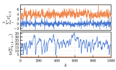
Figure 3: Two feedback simulations of (6), over (18) and (19): first, with a regular LQR control $u_{k}=-K\hat{x}_{k\mid k}$ applied in feedback (blue), while the second employs an the LQR control of the lifted state $u_{k}=-K_{\Psi}\eta_{k}$ (orange). Top is the sum of the state entries,and bottom is the trace of the covariance matrix $\Sigma_{k\mid k}$, for each simulation.

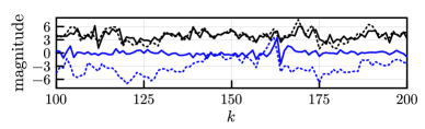
Figure 4: Same feedback simulations as in Fig. 3, but including the hidden true state (which is known in the simulation settings). Each of the above curves is the sum of the entries of the corresponding state: the solid lines are the eKF’s $x_{k\mid k}$; the dotted lines are the true state, while the colors: blue uses $K$ in feedback, and black uses $K_{\Psi}$.

Table 1: Control performance and estimation quality: $K$ vs. $K_{\Psi}$.
Metric (averaged per time-step)	CE “$K$”	lifted “$K_{\Psi}$”	reduction
Achieved cost	$20.7$	$1.87$	$91\%$
Estimation squared error	$32.1$	$0.71$	$98\%$

V Conclusion

The proposed approach for SOC needs the eKF to be an accurate state estimator for the problem at hand, and for the wide-sense approximation it provides (mean and covariance) to be a ‘good enough’ representation of the state uncertainty. For systems with more complex uncertainty descriptions, an alternative filter might be required. Our methodology is also contingent, in its linearization part, on the choice of the dictionary functions used, and hence, on the prediction accuracy of the computed approximate Koopman operator. Therefore, the future of SOC, at least for problems with tractable Bayesian filters, will benefit immediately from all advancements in the Koopman operator theory for control.

We seek further investigations towards exploiting the algebraic structure of the eKF and incorporating deep learning and other state of the art embedding approaches [28] to address large-scale SOC problems.

Government License: The submitted manuscript has been created by UChicago Argonne, LLC, Operator of Argonne National Laboratory (“Argonne”). Argonne, a U.S. Department of Energy Office of Science laboratory, is operated under Contract No. DE-AC02-06CH11357. The U.S. Government retains for itself, and others acting on its behalf, a paid-up nonexclusive, irrevocable worldwide license in said article to reproduce, prepare derivative works, distribute copies to the public, and perform publicly and display publicly, by or on behalf of the Government. The Department of Energy will provide public access to these results of federally sponsored research in accordance with the DOE Public Access Plan. http://energy.gov/downloads/doe-public-access-plan.

References

- [1] A. A. Feldbaum, “Dual control theory. i,” Avtomatika i Telemekhanika, vol. 21, no. 9, pp. 1240–1249, 1960.
- [2] K. J. Åström, Introduction to stochastic control theory. Courier Corporation, 2012.
- [3] P. R. Kumar and P. Varaiya, Stochastic systems: Estimation, identification, and adaptive control. SIAM, 2015.
- [4] E. Tse, Y. Bar-Shalom, and L. Meier, “Wide-sense adaptive dual control for nonlinear stochastic systems,” IEEE Transactions on Automatic Control, vol. 18, no. 2, pp. 98–108, 1973.
- [5] G. Marafioti, R. R. Bitmead, and M. Hovd, “Persistently exciting model predictive control,” International Journal of Adaptive Control and Signal Processing, vol. 28, no. 6, pp. 536–552, 2014.
- [6] M. S. Ramadan, M. Alsuwaidan, A. Atallah, and S. Herbert, “A control approach for nonlinear stochastic state uncertain systems with probabilistic safety guarantees,” arXiv preprint arXiv:2309.08767, 2023.
- [7] F. Kendoul, “Survey of advances in guidance, navigation, and control of unmanned rotorcraft systems,” Journal of Field Robotics, vol. 29, no. 2, pp. 315–378, 2012.
- [8] Z. Jiang, W. Zhou, H. Li, Y. Mo, W. Ni, and Q. Huang, “A new kind of accurate calibration method for robotic kinematic parameters based on the extended kalman and particle filter algorithm,” IEEE Transactions on Industrial Electronics, vol. 65, no. 4, pp. 3337–3345, 2017.
- [9] S. Chen, “Kalman filter for robot vision: a survey,” IEEE Transactions on industrial electronics, vol. 59, no. 11, pp. 4409–4420, 2011.
- [10] E. Ghahremani and I. Kamwa, “Dynamic state estimation in power system by applying the extended kalman filter with unknown inputs to phasor measurements,” IEEE Transactions on Power Systems, vol. 26, no. 4, pp. 2556–2566, 2011.
- [11] S. P. Boyd and L. Vandenberghe, Convex optimization. Cambridge university press, 2004.
- [12] A. Wills, T. B. Schön, L. Ljung, and B. Ninness, “Identification of hammerstein–wiener models,” Automatica, vol. 49, no. 1, pp. 70–81, 2013.
- [13] J. B. Rawlings, D. Q. Mayne, and M. Diehl, Model predictive control: theory, computation, and design, 2nd ed. Nob Hill Publishing Madison, WI, 2017.
- [14] S. Resnick, A probability path. Springer, 2019.
- [15] B. D. Anderson and J. B. Moore, Optimal filtering. Courier Corporation, 2012.
- [16] B. F. La Scala, R. R. Bitmead, and M. R. James, “Conditions for stability of the extended kalman filter and their application to the frequency tracking problem,” Mathematics of Control, Signals and Systems, vol. 8, pp. 1–26, 1995.
- [17] A. H. Jazwinski, Stochastic processes and filtering theory. Courier Corporation, 2007.
- [18] K. Reif, S. Gunther, E. Yaz, and R. Unbehauen, “Stochastic stability of the discrete-time extended kalman filter,” IEEE Transactions on Automatic control, vol. 44, no. 4, pp. 714–728, 1999.
- [19] S. L. Brunton, M. Budišić, E. Kaiser, and J. N. Kutz, “Modern koopman theory for dynamical systems,” arXiv preprint arXiv:2102.12086, 2021.
- [20] D. Bruder, X. Fu, and R. Vasudevan, “Advantages of bilinear koopman realizations for the modeling and control of systems with unknown dynamics,” IEEE Robotics and Automation Letters, vol. 6, no. 3, pp. 4369–4376, 2021.
- [21] L. C. Iacob, R. Tóth, and M. Schoukens, “Koopman form of nonlinear systems with inputs,” Automatica, vol. 162, p. 111525, 2024.
- [22] M. Schatzman, Numerical analysis: a mathematical introduction. Oxford University Press, USA, 2002.
- [23] M. Korda and I. Mezić, “Linear predictors for nonlinear dynamical systems: Koopman operator meets model predictive control,” Automatica, vol. 93, pp. 149–160, 2018.
- [24] M. Haseli and J. Cortés, “Invariance proximity: Closed-form error bounds for finite-dimensional koopman-based models,” arXiv preprint arXiv:2311.13033, 2023.
- [25] G. Mamakoukas, I. Abraham, and T. D. Murphey, “Learning stable models for prediction and control,” IEEE Transactions on Robotics, 2023.
- [26] A. R. Liu and R. R. Bitmead, “Stochastic observability in network state estimation and control,” Automatica, vol. 47, no. 1, pp. 65–78, 2011.
- [27] U. Vaidya, “Observability gramian for nonlinear systems,” in 2007 46th IEEE conference on decision and control. IEEE, 2007, pp. 3357–3362.
- [28] M. Tiwari, G. Nehma, and B. Lusch, “Computationally efficient data-driven discovery and linear representation of nonlinear systems for control,” IEEE Control Systems Letters, 2023.