Strong correlations in matter promote a landscape of ground states and the associated quantum critical points. For metallic systems, there is increasing recognition that the quantum criticality goes beyond the standard Landau framework and, thus, novel means are needed to characterize the quantum critical fluid. Here we do so by studying the entanglement properties near a quantum critical point of a strongly correlated metal. We calculate the mutual information and quantum Fisher information of an Anderson/Kondo lattice model across its Kondo destruction quantum critical point, with the former measuring the bipartite entanglement between two subsystems and the latter serving as witness for multipartite entanglement in the entire system. The mutual information between the conduction electrons and local moments reveals a dynamical effect of Kondo correlations across the quantum critical point. Moreover, the quantum Fisher information of the spin degree of freedom peaks at the quantum critical point and indicates a strongly entangled ground state. Our work opens a new avenue to advance the understanding of metallic quantum criticality by entanglement means in a broad range of strongly correlated systems, and reveals a new regime of quantum matter to witness amplified entanglement.

Introduction.   Quantum entanglement refers to the entwining of particles such that the quantum state of one cannot be completely described without considering those of the others. This interconnection, lacking a classical counterpart, exhibits nonlocal properties that defy conventional understanding ^{1, 2, 3}. In condensed matter settings, entanglement can be crucial to strongly correlated electron systems. For example, collective quantum phases of matter such as the quantum spin liquids and fractional quantum Hall state are theoretically expected to have strongly entangled ground states ^{4, 5, 6, 7}. Strange metals that develop near a quantum critical point (QCP) are also expected to possess enhanced entanglement, though this feature has hardly been studied theoretically and its experimental evidence is lacking ^{8, 9}.

The issue has recently become particularly pressing. For example, even though the QCP of the canonical heavy fermion metal YbRh₂Si₂ is magnetic [antiferromagnetic (AF), to be precise] in nature, involving a zero-temperature transition between AF and paramagnetic metallic phases, the charge response is found to be critical at the QCP ¹⁰. Such a property likewise arises theoretically in the Kondo lattice model ¹¹. The behavior raises the question of whether an enhanced quantum entanglement may be at the origin ^{10, 11, 9, 12}. The theory for quantum criticality in this class of strongly correlated metals goes beyond the Landau framework of order-parameter fluctuations in the form of a Kondo destruction ^{13, 14, 15}.

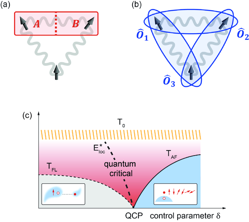
Figure 1: Illustration of mutual information, quantum Fisher information and Kondo destruction quantum critical point.  (a) Mutual information that detects the entanglement between two subsystems $A$ and $B$. (b) Quantum Fisher information defined for local operators $\widehat{\cal O}_{1}$, $\widehat{\cal O}_{2}$, $\widehat{\cal O}_{3}$ witnesses the multipartite entanglement in the entire system. (c) Kondo destruction quantum criticality of a Kondo lattice ⁴². The Kondo destruction energy scale $E_{\text{loc}}^{*}$ vanishes at the QCP. Here, $T_{\text{AF}}$, $T_{\text{FL}}$ and $T_{0}$ are the temperatures of the AF ordering transition, the crossover into the Fermi liquid and the initial onset of Kondo correlations, respectively.

Here we utilize two quantities, the mutual information [Fig. 1(a)] and quantum Fisher information (QFI) [Fig. 1(b)], to analyze the entanglement behavior near a Kondo destruction QCP [Fig. 1(c)]. Our focus is on the Anderson lattice model (see below). We show that the mutual information between the conduction and local electrons remains nonzero as the Kondo destruction QCP is crossed, which characterizes a “dynamical Kondo effect”. At the same time, the QFI of the spin operator is found to peak at the QCP, with behavior that indicates a highly entangled ground state.

Entanglement and its Witness.   Fig. 1(a)(b) illustrate these two entanglement quantities. Qualitatively, the mutual information involves two partitioned subsystems $A$ and $B$ [see the Methods and the Supplementary Information (SI)] [Fig. 1(a)]. The QFI, on the other hand, uses the witnessing operators ($\widehat{\cal O}_{i}$) to serve the purpose of partition. While the entanglement entropy (including the mutual information) is an effective measure of entanglement, a protocol of how to experimentally measure it in many-body settings has yet to be established, progress in mesoscopic systems notwithstanding  ^{16, 17}. By comparison, the QFI is an entanglement witness. Like the Bell’s inequality for the bipartite entanglement of qubits through correlation functions ^{1, 2}, the QFI probes the multipartite entanglement in quantum many-body settings ^{18, 19, 20}; protocols for measuring the QFI have been advanced in terms of inelastic neutron scattering ^{20, 21, 22, 23}, the resonant inelastic X-ray scattering (RIXS) ²⁴ and the angle-resolved photoemission spectroscopy (ARPES) ²⁵.

Kondo Destruction Quantum Critical Point.   The Kondo lattice– and the strongly-coupled Anderson lattice – model contains two types of degrees freedom: a lattice of local moments and a band of conduction electrons (see the Methods). The spins of the local moments and conduction electrons are coupled by the Kondo interaction, whereas the local moments are coupled by the Rudermana-Kittel-Kasuya-Yosida (RKKY) interaction ^{13, 14, 15, 26}. Typically, both types of interactions are AF. The competition between them has been shown ^{13, 14, 15, 9, 27} to yield quantum phase transitions that involve a heavy Fermi liquid phase and a Kondo destruction phase [Fig. 1(c)]. In the heavy Fermi liquid phase, where the Kondo coupling wins over the RKKY interaction, the formation of Kondo singlets between the local spins and conduction electrons gives rise to a large Fermi surface. On the other hand, when the RKKY interaction dominates, the correlations among the local spins are detrimental to the formation of any Kondo singlet. As such, the Kondo destruction QCP where the RKKY and Kondo interactions have the strongest competitions, the degree of entanglement among the local spins and conduction electrons represents an intriguing question. The entanglement entropy has been studied in the past for Kondo systems, for models that involve the local moments at the level of either impurity  ^{28, 29, 30, 31, 32} or lattice ³³. However, with rare exception ³⁴, the QCP of the Kondo lattice systems has not been characterized by any entanglement property.

Mutual Information and Dynamical Kondo Effect.   To capture the Kondo effect in a Kondo lattice system, we consider the $f$ and $c$ electrons at the same site ^{33, 34}. The corresponding mutual information (see the Methods) is defined as

$$I_{f,c}=-S(\rho_{f,c})+S(\rho_{f})+S(\rho_{c}),$$ (1)

where $\rho_{f,c}$ denotes the density matrix of the $f$ and $c$ electrons after tracing out the environment, and $\rho_{f}=\operatorname{tr}_{c}\rho_{f,c}$ ($\rho_{c}=\operatorname{tr}_{f}\rho_{f,c}$) is the reduced density matrix of the $f$($c$) electrons. For definiteness, we consider a square lattice by keeping the nearest neighbor RKKY interaction. Accordingly, the wavevector dependence of the RKKY interaction has the following form: $I_{\bm{q}}=I(\cos q_{x}+\cos q_{y})$. At the ordering wavevector $\bm{q}=\bm{Q}=(\pi,\pi)$, $I_{\bm{Q}}=-2I$.

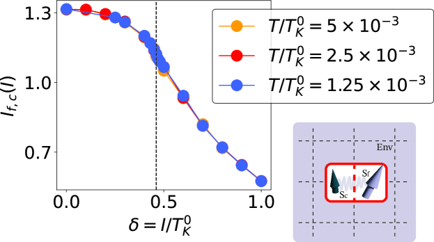
Figure 2: Mutual information between the local $f$ and $c$ electrons.  Evolution of the mutual information of local $f$ and $c$ electrons with the tuning parameter $\delta=I/T_{K}^{0}$. The vertical dashed line indicates the QCP. The schematic diagram of this mutual information is depicted on the right bottom corner, where “Env” stands for the rest of the system (the environment).

In Fig. 2, we show the evolution of $I_{f,c}$ with respect to the non-thermal parameter ($\delta$) that tunes the phase diagram of the Kondo lattice, namely the ratio of the RKKY interaction $I$ to the bare Kondo temperature scale, $T_{K}^{0}$. As this tuning parameter increases, the system undergoes a Kondo destruction quantum phase transition, and the vertical dashed line marks the QCP. In the Kondo-screened phase, the local $f$ electron is strongly bounded with the condution electrons, leading to a large value of mutual information [Fig. 1(c)]. The mutual information is then monotonically decreased as the increasing of RKKY interaction in particular after the system gets into the ordered phase. Surprisingly, in the Kondo-destroyed side [Fig. 1(c)] at $\delta>\delta_{c}$, even though the Kondo singlet is destroyed in the ground state, the mutual information $I_{f,c}$ remains non-zero. This result indicates that the persistence of Kondo-singlet correlations and demonstrates a dynamical Kondo effect when a static Kondo singlet is not formed in the ground. Our result sets the stage to probe quantum entanglement when the QCP is approached from both the Kondo-screened and Kondo-destroyed sides. To do so, we turn to a quantum witness.

Quantum Fisher Information – General.   The essence of the mutual information is the entanglement between subsystems A and B. A different way to detect such entanglement is by measuring the covariance $\operatorname{tr}((\rho_{AB}-\rho_{A}\otimes\rho_{B}){\widehat{\cal O}}_{A}{\widehat{\cal O}}_{B})$ where the operator ${\widehat{\cal O}}_{A/B}$ acts on the A/B subsystem. This correlation witnesses the entanglement between the two subsystems with a proper choice of operators, a notion that has only rarely been considered for condensed matter systems.

To set the stage for the calculations we report below, we motivate how summing over all the covariance of site pairs leads to the QFI, and elaborate on how the QFI can witness the multipartite entanglement and be measured in experiments. The clearest case arises in a pure state, for which the QFI is defined as the variance function $F_{Q}=4\text{Var}({\widehat{\cal O}})\equiv 4(\langle{\widehat{\cal O}}^{2}\rangle-\langle{\widehat{\cal O}}\rangle^{2})$ (see the SI, Sec. I.A). Consider a lattice consisting of $N$ sites, and the operator ${\widehat{\cal O}}=\sum_{i=1}^{N}{\widehat{\cal O}}_{i}$ where each operator ${\widehat{\cal O}}_{i}$ acts only on site $i$. We find (as derived in the SI, Sec. I.B) that the QFI is written as follows:

$$\frac{F_{Q}}{4}=\sum_{i=1}^{N}\text{Var}({\widehat{\cal O}}_{i})+\sum_{i,j\neq i}\operatorname{tr}\left(\left(\rho_{ij}-\rho_{i}\otimes\rho_{j}\right){\widehat{\cal O}}_{i}\otimes{\widehat{\cal O}}_{j}\right)$$ (2)

where $\rho_{i}=\operatorname{Tr}_{j\neq i}\rho$ and $\rho_{ij}=\operatorname{tr}_{l\neq i,j}\rho$. The second term in Eq. (2) measures the difference between $\rho_{ij}$ and $\rho_{i}\otimes\rho_{j}$ which is non-vanishing if the states on site $i$ and $j$ are entangled. We recognize that the mutual information captures the difference between $\log(\rho_{ij})$ and $\log(\rho_{i}\otimes\rho_{j})$ [See the Methods, Eq. (12)]. Thus, the QFI measures the sum of pairwise entanglement between all pairs of sites, which contains the information of multipartite entanglement.

For calculations at nonzero temperatures, we consider the case of a mixed state $\rho$. The QFI is defined for the hermitian operator $\mathcal{O}$; with the spectral decomposition $\rho=\sum_{\lambda_{n}}\lambda_{n}|\lambda_{n}\rangle\langle\lambda_{n}|$, it is expressed as ^{20, 19}

$$F_{Q}=2\sum_{nm}\frac{(\lambda_{n}-\lambda_{m})^{2}}{\lambda_{n}+\lambda_{m}}{\mathcal{O}}_{nm}{\mathcal{O}}_{mn}.$$ (3)

where ${\mathcal{O}}_{nm}=\langle\lambda_{n}|{\widehat{\cal O}}|\lambda_{m}\rangle$. Further details about the QFI are introduced in the SI, Sec. I. The QFI of mixed states at temperature $T$ can be fully determined by the susceptibility of operator $\widehat{\cal O}$ via ²⁰

$$F_{Q}=\frac{2}{\pi}\int_{-\infty}^{\infty}\tanh{\frac{\omega}{2T}}\chi^{\prime\prime}_{\widehat{\cal O}}(\omega)d\omega$$ (4)

where $\chi^{\prime\prime}_{\widehat{\cal O}}(\omega)$ is the imaginary part of the susceptibility $\chi_{\widehat{\cal O}}(\omega)=i\int^{\infty}_{0}dte^{i\omega t}\operatorname{tr}\left(\rho[{\widehat{\cal O}}(t),{\widehat{\cal O}}(0)]\right)$.

To proceed further, we will utilize an important property about the bound of the QFI, which is in the same spirit as Bell’s inequality. Assume ${\widehat{\cal O}}=\sum_{i=1}^{N}{\widehat{\cal O}}_{i}$ and a mixed state of dimension $N$ where ${\widehat{\cal O}}_{i}$ acts on the $i$-th particle (basis vector). If the ground state can be written as the product of some $k$-partite entangled states with $k\leq m$, the QFI density $f_{Q}=F_{Q}/N$ is bounded above by: $f_{Q}\leq m(h_{\text{max}}-h_{\text{min}})^{2}$, where $h_{\text{max/min}}$ is the maximal/minimal eigenvalue of the operator ${\widehat{\cal O}}_{i}$ (see the SI, Sec. I.C). Consequently, if

$$f_{Q}>m(h_{\text{max}}-h_{\text{min}})^{2},$$ (5)

it witnesses the existence of at least $m+1$-partite entangled states in the system ¹⁸. In the remainder of this work, we focus on spin-$1/2$ systems whose normalized QFI density $f_{Q}/(h_{\text{max}}-h_{\text{min}})^{2}=f_{Q}$.

Quantum Fisher Information near the Kondo Destruction Quantum Critical Point.   We are now in position to present the results of our calculation on the QFI in the Kondo lattice system. We focus on the spin operator at the AF wavevector $\bm{Q}$, $\widehat{\cal O}=\sum_{i}S^{z}_{i}e^{i\bm{Q}\cdot\bm{R}_{i}}$. The normalized QFI density is

$$f_{Q}=\frac{2}{\pi}\int_{-\infty}^{\infty}\tanh\frac{\omega}{2T}\chi^{\prime\prime}(\bm{Q},\omega)d\omega,$$ (6)

where $\chi^{\prime\prime}(\bm{Q},\omega)$ is the dynamical spin susceptibility at wave vector $\bm{Q}$. [Note that $\chi^{\prime\prime}(Q,\omega)=\chi^{\prime\prime}_{\widehat{\cal O}}(\omega)/N$.] In practice, the Monte Carlo simulation of the equations in the extended dynamical mean field theory (EDMFT) (see the Methods) is performed on the imaginal frequency axis, and the lattice spin susceptibility at momentum $\bm{q}$ is calculated by

$$\chi(\bm{q},i\omega_{n})=\frac{1}{I_{\bm{q}}+M(i\omega_{n})},$$ (7)

with $M(i\omega_{n})$ being the spin cumulant. We carry out an analytical continuation to obtain the imaginary part of the spin susceptibility in real frequency [for details, see the SI, Sec. III]. Fig. 2(b) shows the imaginary part of the AF dynamical spin susceptibility ${\it Im}\chi(\bm{Q},\omega)$ at the QCP, which is obtained by a Padé decomposition. The lower-frequency part of the curve follows a power law scaling behavior with an anomalous critical exponent $\gamma_{s}\approx 0.82$, which is a salient feature of the Kondo destruction QCP ¹³.

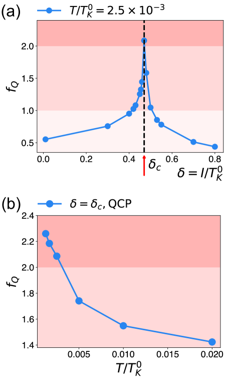
Figure 4: The normalized Quantum Fisher information density.   (a) The low-temperature normalized QFI density as a function of the tuning parameter $\delta=I/T_{K}^{0}$. The vertical dashed line and the red arrow indicate the location of the QCP. The normalized QFI density is peaked at the QCP, where it exceeds $2$, indicating that the ground state contains at least three-partite entanglement. The dark (light) red shading, here and in panel (b), marks the regime where the system is at least $3$- ($2$-) partite entangled. (b) The normalized QFI density vs. temperature $T$ (normalized by the bare Kondo temperature, $T_{K}^{0}$) at the quantum critical coupling, $\delta_{c}=I_{c}/T_{K}^{0}$. The normalized QFI density monotonically increases with the decrease of temperature. The data are obtained in the quantum critical regime with $\delta_{c}=0.47$, except for the lowest temperature $T=1.25\times 10^{-3}$, which requires a finer tuning to reach quantum criticality and is calculated at $\delta_{c}=0.465$.

We show the normalized QFI density, at a very low temperature ($T=2.5\times 10^{-3}T_{K}^{0}$), versus the tuning parameter $\delta=I/T_{K}^{0}$ in Fig. 4(a), where the vertical dashed line marks the QCP. The left and right sides of the QCP correspond to the Kondo screened phase and Kondo destroyed phase [Fig. 1(c)], respectively. We find $f_{Q}$ to display a sharp peak at the QCP, reaching the value around $2.2$. This peak exceeds the bound of $2$, indicating that the ground state contains at least three-partite entanglement according to Eq. (5).

We next fix the system to be at $\delta=\delta_{c}$ and change the temperature (with the QCP located at $T=0)$. As shown in Fig. 4(b), the normalized QFI density monotonically increases with decreasing temperature and reaches the same low-temperature regime of at least three-partite entanglement.

To probe further the entanglement, we compute the two-tangle of spin pairs, which is a measure of the entanglement between two spins ³⁵ (see the SI, Sec. II). At the QCP where the spin parity and translation symmetry are preserved and the magnetic order vanishes, the two-tangle is expressed as $\tau_{0\mathbf{R}}=|\max\{0,-\frac{1}{2}\pm 2\langle\mathbf{S}_{0}\cdot\mathbf{S}_{\mathbf{R}}\rangle\}|^{2}$ (Refs. 36, 22), in which the correlation function $\langle\mathbf{S}_{0}\cdot\mathbf{S}_{\mathbf{R}}\rangle=\frac{1}{\pi N_{\bm{q}}}\sum_{\bm{q}}e^{i\bm{q}\mathbf{R}}\int d\omega\chi(\bm{q},\omega)$.

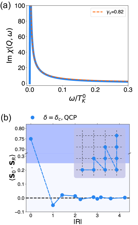
Figure 3: Spin-spin correlation functions at the QCP.    (a) The AF dynamical spin susceptibility in real frequency, at the QCP ($\delta=\delta_{c}$), is obtained by an analytical continuation from $\chi(\bm{Q},i\omega_{n})$, which is simulated by the Monte Carlo method. The blue line denotes the ${\it Im}\chi(\bm{Q},\omega)$ at $T/T_{K}^{0}=2.5\times 10^{-3}$ obtained from the Pade decomposition, which peaks in the vicinity of $\omega\sim T$. The lower frequency part of the curve follows a power law scaling with critical exponent $\gamma_{s}\sim 0.82$. (b) The equal-time correlation function $\langle\mathbf{S}_{0}\cdot\mathbf{S}_{\mathbf{R}}\rangle$ at the QCP ($\delta=\delta_{c}$). Since $|\langle\mathbf{S}_{0}\cdot\mathbf{S}_{\mathbf{R}}\rangle|<0.25$ for all $\mathbf{R}\neq 0$, the two-tangle is zero: there is no pairwise entanglement. The inset displays the lattice sites $\mathbf{R}$ we select for the calculation.

We present this correlation function in Fig. 3(b). It is evident that $\tau_{0\mathbf{R}}=0$ for every pair of spins. Since our QFI reveals multipartite entanglement in the system, the vanishing two-tangles mean that the entanglement is distributed among multiple spins rather than being confined to pairwise spins. It is in agreement with the quantum monogamy and the Coffman-Kundu-Wootters inequality ^{3, 37}. For example, a maximally entangled state of spins with entanglement distributed among all spins have no entanglement inside any subspace. The combination of a mutipartite QFI and vanishing two-tangle provide evidence for strong entanglement in the system.

Discussion and Connection with Experiment.   Several points are in order. First, the QFI of the spin degrees of freedom is determined from spin-spin correlation functions. As such, it can be experimentally determined by inelastic neutron scattering experiments. Indeed, our theoretical results are qualitatively consistent with the quantum Fisher information that is determined in a forthcoming experimental work in Kondo destruction quantum critical heavy fermion metals (F. Mazza et al., private communication). In wider condensed matter contexts, the normalized QFI density has only been measured in several insulating quantum magnets. The value we have calculated for the Kondo destruction QCP is comparable to that determined in candidate materials for such highly entangled ground states as two-dimensional spin liquids ($3.4$ for $\rm KYbSe_{2}$, Ref. 22) and one-dimensional Heisenberg spin-$1/2$ chain ($1.9$ for KCuCl₃, Ref. 23), respectively.

Second, while the QFI of the spin degrees of freedom reflects the dynamical spin susceptibility, it encodes information beyond the usual characterization of the latter in condensed matter settings. The key is the QFI bounds. Based on the bounds, the QFI characterizes the system’s multipartite entanglement. This is in the same spirit that the Bell’s inequality contains information (about bipartite entanglement) beyond the correlation function per se.

Finally, the metallic nature of the strange metal systems allows to study the QFI of other degrees of freedom, such as the charge and single particle. With growing proposals for measuring the QFIs from other spectroscopies such as RIXS ²⁴ and ARPES ²⁵, there is considerable prospect for further theoretical and experimental studies of multipartite entanglement in strange metals.

Summary.    We have studied bipartite and multipartite entanglement near quantum criticality in a strongly correlated metal. Our results characterize the Kondo destruction quantum critical point of a Kondo lattice model. The mutual information between the conduction electrons and local moments is found to stay nonzero when the system is tuned through the quantum critical point into its Kondo destruction phase, which captures the dynamical effect of the Kondo correlations across the quantum critical point. The quantum Fisher information, in combination with the two tangles, reveal amplified entanglement at the quantum critical point. Our work represents the first theoretical entanglement characterization of quantum critical strange metals and, as such, showcases a new window into the quantum correlations that underlie a wide range of strongly interacting metallic systems. More generally, our work points to broad classes of gapless quantum matter with strange metallicity as a promising setting to witness enhanced entanglement.

Methods
Quantum criticality in the Anderson lattice model.   We consider the $\mathrm{SU(2)}$ periodic Anderson lattice model, which takes the form:

$$H =\frac{U}{2}\sum_{i}\left[\sum_{\sigma}f_{i,\sigma}^{\dagger}f_{i,\sigma}-1\right]^{2}+\sum_{ij}I_{ij}\bm{S}_{i}\cdot\bm{S}_{j}$$ (8)

$$+V\sum_{i,\sigma}\left(c_{i,\sigma}^{\dagger}f_{i,\sigma}+f_{i\sigma}^{\dagger}c_{i,\sigma}\right)+\sum_{p,\sigma}\epsilon_{p}c^{\dagger}_{p,\sigma}c_{p,\sigma}.$$

Here, $f_{i\sigma}^{\dagger}$ ($c_{i\sigma}^{\dagger}$) creates a local (conduction) electron with spin $\sigma$ at site $i$. The hybridization $V$ couples the local $f$-electron with the conduction $c$-electron, which has a dispersion $\epsilon_{p}$. Moreover, the on-site Coulomb repulsion is represented by $U$. When $U$ is sufficiently large, the model is equivalent to the Kondo lattice Hamiltonian, with a Kondo couping $J_{K}\sim\frac{4V^{2}}{U}$. Finally, $\bm{S}_{i}=f^{\dagger}\frac{\bm{\sigma}}{2}f$ represents the spin operator of the local moment, and $I_{ij}$ describes the AF RKKY interaction between the local moments. We consider an RKKY interaction $I_{ij}$. Its Fourier transformation, $I_{\bm{q}}$, reaches the most negative value at the AF wave vector $\bm{Q}$, with $I_{\bm{Q}}=-2I$.

We treat the Hamiltonian described in Eq. (8) by the extended dynamical mean-field (EDMFT) method, within which the dynamical competition between the Kondo hybridization and RKKY interaction is taken into account appropriately ^{38, 39, 40, 41}. Through EDMFT, the correlation functions of the lattice model can be calculated in terms of those of a self-consistent Bose-Fermi Anderson (BFA) model, in which the local $f$ electron couples with a fermionic bath and a bosonic bath. The fermioninic bath comes from the hybridization with the conduction electrons and the bosonic bath describes the spin fluctuations from the RKKY interaction. The action after integrating out both baths takes the form:

$$S_{BFA} =\int_{0}^{\beta}d\tau\left[\sum_{\sigma}f_{\sigma}^{\dagger}\partial_{\tau}f_{\sigma}+h_{loc}S^{z}+\frac{U}{2}\left(n_{f}-1\right)^{2}\right]$$ (9)

$$-\int_{0}^{\beta}d\tau d\tau^{\prime}\bigg{[}\sum_{\sigma}f_{\sigma}^{\dagger}(\tau)V^{2}\mathcal{G}_{c}(\tau-\tau^{\prime})f_{\sigma}$$

$$+\frac{1}{2}\sum_{\alpha}S^{\alpha}[\chi_{0}^{-1}(\tau-\tau^{\prime})]S^{\alpha}(\tau^{\prime})\bigg{]},$$

where $\beta=1/T$ and $n_{f}=\sum_{\sigma}f_{\sigma}^{\dagger}f_{\sigma}$. We set $\hbar=k_{B}=1$ throughout this work. The static Weiss field $h_{loc}$ is introduced to capture the AF order, while $\mathcal{G}_{c}$ and $\chi_{0}$ denote the Green’s function of the fermionic and bosonic bath, respectively. For the bosonic bath, $\alpha\in\{x,y,z\}$. The self-consistent conditions are:

$$\chi_{loc}^{\alpha}(i\omega_{n}) =\int d\epsilon\frac{\rho_{I}(\epsilon)}{\epsilon+M^{\alpha}(i\omega_{n})}$$ (10)

$$M^{\alpha}(i\omega_{n}) =[\chi_{0}^{\alpha}](i\omega_{n})+1/\chi_{loc}^{\alpha}(i\omega_{n})$$

$$\mathcal{G}_{c}(i\omega_{n}) =\int d\epsilon\frac{\rho_{0}(\epsilon)}{-i\omega_{n}+\epsilon+\Sigma_{c}(i\omega_{n})}$$

$$h_{loc} =-[2I-\chi_{0}^{\alpha}](i\omega_{n}=0)]m_{AF}.$$

Here, $\rho_{I}(\epsilon)$ represents the RKKY density of states, which is obtained from $\rho_{I}(\epsilon)=\sum_{\bm{q}}\delta(\epsilon-I_{\bm{q}})$. We consider a generic density of the conduction electrons ($\rho_{0}$) with a nonzero value at the Fermi energy.

Mutual information.   Mutual information measures the information between two subsystems. Consider a subspace $A\times B\subset M$ where $M$ is the entire manifold of the parameter space of the system, the mutual information of a mixed state $\rho_{AB}$ on this space is defined by ²

$$I(A;B):= S(\rho_{A})+S(\rho_{B})-S(\rho_{AB})$$ (11)

$$\equiv \operatorname{tr}\left(\rho_{AB}(\log(\rho_{AB})-\log(\rho_{A}\otimes\rho_{B}))\right)$$ (12)

where $\rho_{A}=\operatorname{tr}_{B}\rho_{AB}$, $\rho_{B}=\operatorname{tr}_{A}\rho_{AB}$ and $S(\rho)=-\operatorname{tr}(\rho\log\rho)$ is the von Neumann entropy.

Data availability
The data that support the findings of this study are available from the corresponding author upon reasonable request.

Code availability
The computer codes that were used to generate the data that support the findings of this study are available from the corresponding author upon reasonable request.

^† These authors contributed equally.

Acknowledgment:   We thank Gabriel Aeppli and Matthew Foster for useful discussions. Work at Rice has primarily been supported by the the NSF Grant No. DMR-2220603, the AFOSR Grant No. FA9550-21-1-0356, the Robert A. Welch Foundation Grant No. C-1411, and the Vannevar Bush Faculty Fellowship ONR-VB N00014-23-1-2870. The majority of the computational calculations have been performed on the Shared University Grid at Rice funded by NSF under Grant EIA-0216467, a partnership between Rice University, Sun Microsystems, and Sigma Solutions, Inc., the Big-Data Private-Cloud Research Cyberinfrastructure MRI-award funded by NSF under Grant No. CNS-1338099, and the Extreme Science and Engineering Discovery Environment (XSEDE) by NSF under Grant No. DMR170109. H.H. acknowledges the support of the European Research Council (ERC) under the European Union’s Horizon 2020 research and innovation program (Grant Agreement No. 101020833). Work in Vienna was supported by the Austrian Science Fund (projects I 5868-N - FOR 5249 - QUAST and and SFB F 86, Q-M$\&$S) and the ERC (Advanced Grant CorMeTop, No. 101055088). Several of us (Y.F., M.M., Y.W., L.C., S.P., Q.S.) acknowledge the hospitality of the Kavli Institute for Theoretical Physics, supported in part by the National Science Foundation under Grant No. NSF PHY1748958, during the program “A Quantum Universe in a Crystal: Symmetry and Topology across the Correlation Spectrum”. Q.S. acknowledge the hospitality of the Aspen Center for Physics, which is supported by NSF grant No. PHY-2210452.

Author contributions
Q.S. conceived the research. Y.F., M.M., Y.W., L.C., H.H. and Q.S. carried out model studies. Y.F., Y.W., S.P. and Q.S. contributed to understanding the comparison of QFI with experimental measurements. Y.F., M.M., Y.W., L.C. and Q.S. wrote the manuscript, with inputs from all authors.

Competing interests
The authors declare no competing interests.

Additional information
Correspondence and requests for materials should be addressed to Q.S. (qmsi@rice.edu).

Supplemental Information

I Introduction to quantum Fisher information

Because the quantum Fisher information is not widely considered in the condensed matter community, we briefly introduce it here in connection to the present work.

Entanglement is usually hard to detect in the real world. Different from entanglement entropy and mutual information, correlations are much easier to measure. In fact, certain combination of correlation functions can be arranged to witness the entanglement. The first example of such a witness is Bell’s inequality, where a violation of the inequality indicates the existence of the entangled states. Bell’s inequality, though, is designed to distinguish bipartite entangled spin states from states without any entanglement, i.e. separable states. To witness any multipartite entangled states, we rely on the quantum Fisher information, which turns out to be measurable in experiments.

Quantum Fisher information was first proposed in quantum metrology as the quantum version of Fisher information in the classical estimation theory in statistics ^{43, 44, 45, 46}. It is the upper bound of the classical Fisher information in quantum mechanics ^{47, 48}. Therefore, it serves as the quantum Cramér-Rao lower bound ^{45, 46} of the variance of the unbiased estimation of parameter $\theta$, $\text{Var}(\hat{\theta})\geq F^{-1}_{Q}$. It has been found that entanglement can increase the precision of estimations beyond the classical limit ^{49, 19, 46}. Conversely, the quantum Fisher information can also detect the amount of entanglement.

In the following subsection I.1, we will first review the definition of quantum Fisher information and derive the definition Eq. (3) that we used in the main text. In the next subsection I.3, we prove the general upper bound of quantum Fisher information for generic operators.

I.1 The definition of quantum Fisher information

To motivate the quantum Fisher information ^{19, 47}, we consider a process where the density matrix evolves as follows

$$\partial_{a}\rho=\frac{1}{2}(\rho\widehat{L}_{a}+\widehat{L}_{a}\rho).$$ (S1)

Here, $\partial_{a}=\partial/\partial\theta_{a}$, with $\theta_{a}$ parametrizes this process, and $\rho$ is the density matrix. This equation also defines $\widehat{L}_{a}^{\dagger}=\widehat{L}_{a}$ as the symmetric logarithmic derivative (SLD) operator of the density matrix. Associated with this process, the quantum Fisher information matrix is ^{19, 47}

$$F_{ab}:=\frac{1}{2}\operatorname{tr}(\rho\{\widehat{L}_{a},\widehat{L}_{b}\})\,.$$ (S2)

For a pure state $|\psi\rangle$, $\rho^{2}=\rho$. Thus, $\widehat{L}_{a}=2\partial_{a}\rho$ and the quantum Fisher information matrix can be simplified as

$$\widehat{L}_{a} =2(|\psi\rangle\langle\partial_{a}\psi|+|\partial_{a}\psi\rangle\langle\psi|)$$ (S3)

$$F_{ab}(|\psi\rangle) =4\Re(\langle\psi|\partial_{a}\partial_{b}|\psi\rangle-\langle\psi|\partial_{a}|\psi\rangle\langle\psi|\partial_{b}|\psi\rangle)$$ (S4)

where $\Re$ indicates taking the real part. The quantum Fisher information is the diagonal element at $a=\theta$,

$$F_{Q}(|\psi\rangle) =4(\langle\partial_{\theta}\psi|\partial_{\theta}\psi\rangle-|\langle\psi|\partial_{\theta}\psi\rangle|^{2})$$ (S5)

If we consider the unitary process $|\psi\rangle\rightarrow e^{-i\theta\widehat{\mathcal{O}}}|\psi\rangle$, the quantum Fisher information of pure state $|\psi\rangle$ is

$$F_{Q}(|\psi\rangle)=4\text{Var}(\widehat{\mathcal{O}}).$$ (S6)

For mixed states, we can use a spectral decomposition of $\rho=\sum_{i}\lambda_{n}|\lambda_{n}\rangle\langle\lambda_{n}|$ to derive the following expression

$$\langle\lambda_{n}|\partial_{a}\rho|\lambda_{m}\rangle =\frac{\lambda_{n}+\lambda_{m}}{2}\langle\lambda_{n}|\widehat{L}_{a}|\lambda_{m}\rangle$$ (S7)

$$F_{ab} =\sum_{nm}\frac{2\Re(\langle\lambda_{n}|\partial_{a}\rho|\lambda_{m}\rangle\langle\lambda_{m}|\partial_{b}\rho|\lambda_{n}\rangle)}{\lambda_{n}+\lambda_{m}}$$ (S8)

where $\Re$ indicates taking the real part. Eq. (S8) can be further rewritten in terms of eigenstates $|\lambda_{n}\rangle$. By substituting $\partial_{a}\rho=\sum_{i}\partial_{a}\lambda_{n}|\lambda_{n}\rangle\langle\lambda_{n}|+\lambda_{n}|\partial_{a}\lambda_{n}\rangle\langle\lambda_{n}|+\lambda_{n}|\lambda_{n}\rangle\langle\partial_{a}\lambda_{n}|$ and noticing that $\langle\lambda_{n}|\partial_{a}\lambda_{n}\rangle$ is purely imaginary, we get

$$F_{ab}= \sum_{n}\frac{\partial_{a}\lambda_{n}\partial_{b}\lambda_{n}}{\lambda_{n}}$$

$$+2\sum_{nm}\frac{(\lambda_{n}-\lambda_{m})^{2}}{\lambda_{n}+\lambda_{m}}\langle\lambda_{n}|\partial_{a}\lambda_{m}\rangle\langle\partial_{b}\lambda_{n}|\lambda_{m}\rangle$$ (S9)

The quantum Fisher information obtains when the diagonal element $F_{aa}$ at $\theta_{a}$ is taken in this matrix

$$F_{Q}=\sum_{n}\frac{(\partial_{a}\lambda_{n})^{2}}{\lambda_{n}}+2\sum_{nm}\frac{(\lambda_{n}-\lambda_{m})^{2}}{\lambda_{n}+\lambda_{m}}\big{|}\langle\lambda_{n}|\partial_{a}\lambda_{m}\rangle\big{|}^{2}$$ (S10)

The first term vanishes when the state evolves unitarily since the eigenvalues $\lambda_{n}$ do not change. Thus, the second term is the main focus of this work. It describes the fluctuations of the states with respect to the parameter changes.

For the unitary process $|\lambda_{n}\rangle\rightarrow e^{-i\theta_{a}\widehat{\cal O}_{a}}|\lambda_{n}\rangle$, or equivalently $\rho\rightarrow e^{-i\theta_{a}\widehat{\cal O}_{a}}\rho e^{i\theta_{a}\widehat{\cal O}_{a}}$, using the evolution of wavefunction or the density matrix

$$i\partial_{a}|\lambda_{n}\rangle =\widehat{\cal O}_{a}|\psi\rangle$$ (S11)

$$i\partial_{a}\rho =[\widehat{\cal O}_{a},\rho]$$ (S12)

we get the following simplified definition of quantum Fisher information matrix

$$F_{ab}=2\sum_{nm}\frac{(\lambda_{n}-\lambda_{m})^{2}}{\lambda_{n}+\lambda_{m}}{\mathcal{O}}_{a~{}nm}{\mathcal{O}}_{b~{}mn}.$$ (S13)

Taking the diagonal element of this matrix we get Eq. (3) in the main text.

$$F_{Q}=2\sum_{nm}\frac{(\lambda_{n}-\lambda_{m})^{2}}{\lambda_{n}+\lambda_{m}}{\mathcal{O}}_{nm}{\mathcal{O}}_{mn}.$$ (S14)

Instead of taking the derivative of parameters, this definition only rely on the operators. Note, this quantum Fisher information corresponds to the particular unitary process described above. This process can be defined for any hermitian operator $\widehat{\cal O}$. Typical combinations of parameter and operator in such unitary processes include position and momentum operator, angle and angular momentum operator, time and the Hamiltonian operator.

QFI is an additive and convex function of the density matrix given the operator ${\widehat{\cal O}}$ ^{19, 50, 46}, i.e.

$$F_{Q}\left(\sum_{\alpha}p_{\alpha}\rho_{\alpha}\right) \leq\sum_{\alpha}p_{\alpha}F_{Q}(\rho_{\alpha})\leq\max_{|\psi\rangle}F_{Q}(|\psi\rangle)$$ (S15)

where $\sum_{\alpha}p_{\alpha}=1$ is a partition and the maximal value of $F$ is always reached by a pure state as the last inequality shows.

I.2 Local operators detect multipartite entanglement

QFI defined by Eq. (S14) reduces to the variance of operator $\cal O$ for a pure state,

$$\frac{1}{4}F_{Q}(|\psi\rangle)=\text{Var}(\widehat{\cal O})=\langle\psi|\widehat{\cal O}^{2}|\psi\rangle-\langle\psi|\widehat{\cal O}|\psi\rangle^{2}$$ (S16)

If we select the operator as a sum of $N$ independent local operators $\widehat{\cal O}_{i}$, each exclusively acting on each site $i$, i.e. $\widehat{\cal O}=\sum_{i}^{N}\widehat{\cal O}_{i}$, the variance take the following form:

$$\text{Var}(\widehat{\cal O}) =\sum_{i=1}^{N}\langle\widehat{\cal O}_{i}^{2}\rangle-\langle\widehat{\cal O}_{i}\rangle^{2}+\sum_{j}\sum_{i\neq j}\langle\widehat{\cal O}_{i}\widehat{\cal O}_{j}\rangle-\langle\widehat{\cal O}_{i}\rangle\langle\widehat{\cal O}_{j}\rangle$$

$$=\sum_{i}\text{Var}_{i}+\sum_{j}\sum_{i\neq j}\text{Cov}_{ij}$$ (S17)

where the diagonal term $\text{Var}_{i}=\langle\widehat{\cal O}_{i}^{2}\rangle-\langle\widehat{\cal O}_{i}\rangle^{2}$ is the variance of each local operator and the off-diagonal term $\text{Cov}_{ij}=\langle\widehat{\cal O}_{i}\widehat{\cal O}_{j}\rangle-\langle\widehat{\cal O}_{i}\rangle\langle\widehat{\cal O}_{j}\rangle$ is the covariance. The covariance detects the entanglement between sites $i$ and $j$ since it can be written as

$$\text{Cov}_{ij} =\sum_{i\neq j}\operatorname{tr}\left(\rho\widehat{\cal O}_{i}\widehat{\cal O}_{j}\right)-\operatorname{tr}\left(\rho\widehat{\cal O}_{i}\right)\operatorname{tr}\left(\rho\widehat{\cal O}_{j}\right)$$

$$=\operatorname{tr}\left(\rho_{ij}(\widehat{\cal O}_{i}\otimes\widehat{\cal O}_{j})\right)-\operatorname{tr}\left((\rho_{i}\widehat{\cal O}_{i}\otimes\rho_{j}\widehat{\cal O}_{j})\right)$$

$$=\operatorname{tr}\left(\left(\rho_{ij}-\rho_{i}\otimes\rho_{j}\right)\widehat{\cal O}_{i}\otimes\widehat{\cal O}_{j}\right)$$ (S18)

where $\rho=|\psi\rangle\langle\psi|$, $\rho_{i}=\operatorname{tr}_{j\neq i}\rho$ and $\rho_{ij}=\operatorname{tr}_{l\neq i,j}\rho$. The second equality in Eq. (S18) utilizes the fact $\operatorname{tr}A\otimes B=\operatorname{tr}A\operatorname{tr}B$. Eq. (S18) shows that the covariance of two local operators at sites $i$ and $j$ is a measure of $\rho_{ij}-\rho_{i}\otimes\rho_{j}$. Therefore, this term measures the pairwise entanglement between the two sites.

Combining Eqs. (S14) and (S18), we conclude that the variance of $\cal O$, which is the sum of the measurement of pairwise entanglement $\text{Cov}_{ij}$, contains the information of multipartite entanglement of the entire system. Eqs. (S17) and (S18) derive Eq. (2) in the maintext.

In discussing the properties of $\text{Var}(\widehat{\cal O})$ and $\text{Cov}{ij}$, it is important to note two key aspects. First, $\text{Var}(\widehat{\cal O})\geq 0$ while $\text{Cov}_{ij}$ does not have such constraint and can be negative. Secondly, if all local operators $\widehat{\cal O}_{i}$ have identical eigenvalues, these quantities are bounded by

$$\text{Var}(\widehat{\cal O}) \leq N^{2}(h_{\text{max}}-h_{\text{min}})^{2}/4$$ (S19)

$$\text{Var}_{i} \leq(h_{\text{max}}-h_{\text{min}})^{2}/4$$ (S20)

$$|\text{Cov}_{ij}| \leq|h_{\text{max}}-h_{\text{min}}|\times$$

$$\qquad\max\{|h_{\text{max}}|,|h_{\text{min}}|,|h_{\text{max}}+h_{\text{min}}|\}$$ (S21)

where $h_{\text{max/min}}$ is the maximal/minimal eigenvalue of the operators $\widehat{\cal O}_{i}$. The proof of Eq. (S19) and Eq. (S20) is shown in the next subsection I.3. The bound in Eq. (S21) follows that $\langle\widehat{\cal O}_{i}\widehat{\cal O}_{j}\rangle\leq\max\{h_{\text{max}}^{2},h_{\text{min}}^{2}\}$ and $\langle\widehat{\cal O}_{i}\rangle\langle\widehat{\cal O}_{j}\rangle\geq\min\{h_{\text{max}}^{2},h_{\text{min}}^{2},h_{\text{max}}h_{\text{min}}\}$.

I.3 The upper bound of quantum Fisher information

Quantum Fisher information is a positive-semi-definite, additive and convex function of $\rho$ ^{19, 50, 46, 47}

$$F_{Q}\left(\sum_{\alpha}p_{\alpha}\rho_{\alpha}\right) \leq\sum_{\alpha}p_{\alpha}F_{Q}(\rho_{\alpha})\leq\max_{|\psi\rangle}F_{Q}(|\psi\rangle)$$ (S22)

Therefore, the maximum value is realized by a pure state. Now we are interested in the question, what is the upper bound of the quantum Fisher information when the wavefunctions are restricted to be $m$-entangled, which means the density matrix can be decomposed into tensor products

$$\rho=\otimes_{l}\rho_{l}$$ (S23)

where the dimension of each $\rho_{l}$ is no greater than $m$.

For $N$ identical particles with operators $\widehat{\cal O}_{j}$, where $j=1\dots N$, the quantum Fisher information of a pure state at zero temperature is the variance

$$F_{Q}=4\left(\langle\widehat{\cal O}^{2}\rangle-\langle\widehat{\cal O}\rangle^{2}\right)$$ (S24)

where $\widehat{\cal O}=\sum_{j}\widehat{\cal O}_{j}$. We now show that for $m$-entangled states, the quantum Fisher information is bounded by

$$F_{Q}\leq mN(h_{\text{max}}-h_{\text{min}})^{2}$$ (S25)

where $h_{\text{max/min}}$ is the maximal/minimal eigenvalue of the operators $\widehat{\cal O}_{j}$.

While this bound of general operators has appeared in several references ^{25, 23}, we are unaware of a prior demonstration of its proof. Thus, we present one proof of this result here.

Proof.

We first consider the case $N/m\in\mathbb{Z}$. Then the $N$ particles can be divided into $N/m$ copies of $m$-entangled states. Therefore,

$$F_{Q} =4\frac{N}{m}\left(\langle\left(\sum_{j=1}^{m}\widehat{\cal O}_{j}\right)^{2}\rangle-\langle\sum_{j=1}^{m}\widehat{\cal O}_{j}\rangle^{2}\right)$$

$$\leq 4\frac{N}{m}~{}m^{2}\left(\frac{h_{\text{max}}-h_{\text{min}}}{2}\right)^{2}$$

$$=Nm(h_{\text{max}}-h_{\text{min}})^{2}$$ (S26)

where the inequality comes from the maximal variance of the operator $\widehat{\cal O}^{\prime}=\sum_{j=1}^{m}\widehat{\cal O}_{j}$. To see this, consider the spectral decomposition

$$\langle\widehat{\cal O}^{\prime 2}\rangle-\langle\widehat{\cal O}^{\prime}\rangle^{2}=\sum_{n}p_{n}h_{n}^{\prime 2}-(\sum_{n}p_{n}h_{n}^{\prime})^{2}$$

$$\leq ph_{\text{max}}^{\prime 2}+(1-p)h_{\text{min}}^{\prime 2}-(ph_{\text{max}}^{\prime}+(1-p)h_{\text{min}}^{\prime})^{2}$$

$$=-(h_{\text{max}}^{\prime}-h_{\text{min}}^{\prime})^{2}(p^{2}-p)$$

$$\leq\left(\frac{h_{\text{max}}^{\prime}-h_{\text{min}}^{\prime}}{2}\right)^{2}$$

$$\leq m^{2}\left(\frac{h_{\text{max}}-h_{\text{min}}}{2}\right)^{2}$$ (S27)

where $h^{\prime}_{n}$ is the $n$-th eigenvalue of of $\widehat{\cal O}^{\prime}$ and $h^{\prime}_{\text{max/min}}$ is the maximal/minimal eigenvalue of $\widehat{\cal O}^{\prime}$. The first and second inequality in Eq. (S27) derive the maximal variance of a general operator and the last inequality is a consequence of the fact $mh_{\text{min}}\leq h^{\prime}_{\text{min}}\leq h^{\prime}_{\text{max}}\leq mh_{\text{max}}$. Therefore, applying Eq. (S27) to $\widehat{\cal O}^{\prime}$ leads to Eq. (S26).

When $N/m\not\in\mathbb{Z}$, as a consequence of the convexity property ¹⁸, the quantum Fisher information is maximized when the $[\frac{N}{m}]$ sectors of $m$-entangled states and the residual sector of $(N-[\frac{N}{m}]m)$-entangled states are all maximally entangled. This leads to

$$F_{Q}\leq\bigg{(}\big{[}\frac{N}{m}\big{]}m^{2}+r^{2}\bigg{)}(h_{\text{max}}-h_{\text{min}})^{2}$$ (S28)

where $\big{[}\frac{N}{m}\big{]}$ is the integer part of $N/m$ and $r=N-\big{[}\frac{N}{m}\big{]}$. In the case of $N\gg m$, this bound is

$$F_{Q} \leq\bigg{(}Nm+O(m^{2})\bigg{)}(h_{\text{max}}-h_{\text{min}})^{2}$$

$$\xrightarrow[]{N\rightarrow\infty}Nm(h_{\text{max}}-h_{\text{min}})^{2}$$ (S29)

∎

This conclusion works for generic operators. We check that it agrees with spin-$\frac{1}{2}$ chain where the bound is saturated by Greenberger–Horne–Zeilinger (GHZ) states ¹⁸.

II Two-tangle

One-tangle and two-tangle were proposed to be a measure of quantum entanglement in qubits ³⁵. One-tangle is defined as

$$\tau^{(1)}=4\det{\rho_{1}}$$ (S30)

where $\rho_{1}$ is the reduced density matrix tracing out all qubits except the target one. $\tau^{(1)}\in[0,1]$ measures the entanglement between the target qubit and the remaining qubits. When $\tau^{(1)}=0$, the qubit is separable from other qubits; when $\tau^{(1)}=1$, they are maximally entangled.

Two-tangle is defined as

$$\tau=|\max\{0,2\lambda_{\text{max}-\operatorname{tr}R}\}|^{2}$$ (S31)

where $\lambda_{\text{max}}$ is the maximal eigenvalue of matrix $R=\sqrt{\sqrt{\rho}\tilde{\rho}\sqrt{\rho}}$ where $\tilde{\rho}={\cal T}\rho{\cal T}^{-1}$ is the density matrix after spin-flipping. ${\cal T}=\sigma_{y}\otimes\sigma_{y}{\cal K}$ for spin-$1/2$ systems and $\cal K$ is the charge conjugation operator. Two-tangle $\tau\in[0,1]$; it describes the entanglement between two quibits. When $\tau=0$ the two qubits are separable; when $\tau=1$ they are maximally entangled. Two-tangle is also closely related to the entanglement of formation $E_{f}$, which measures the amount of entanglement to prepare a state from completely separable states. The definition of $E_{f}$ and its relation to two-tangle are ³⁵

$$E_{f} =\inf\left\{\sum_{n}p_{n}E_{f}(|\psi_{n}\rangle)\right\}$$ (S32)

$$E_{f} =h\left(\frac{1+\sqrt{1-\tau(\rho)}}{2}\right)$$ (S33)

where the infimum is taken over all possible decomposition of $\rho=\sum_{n}p_{n}|\psi_{n}\rangle\langle\psi_{n}|$ and for pure state $E_{f}(|\psi\rangle_{AB})=S(\rho_{A})=S(\rho_{B})$ is the entanglement entropy. Here $h(x)=-x\log x-(1-x)\log(1-x)$.

Two-tangles satisfy the Coffman-Kundu-Wootters inequality ^{3, 37}

$$\tau_{AA_{1}}+\tau_{AA_{2}}+\dots+\tau_{AA_{n}}\leq\tau_{A(A_{1}A_{2}\dots A_{n})}$$ (S34)

which means the sum of pairewise entanglement between $A$ and $A_{i}$ is no greater than the entanglement between $A$ and the remaining system. This inequality quantifies the concept of quantum monogamy, meaning that if $A$ and $A_{1}$ are maximally entangled (i.e. $\tau_{AA_{1}}=\tau_{A(A_{1}A_{2}\dots A_{n})}=1$), then $A$ can not entangle with other qubits (i.e. $\tau_{AA_{2}}=\dots=\tau_{AA_{n}}=0$).

Two-tangle describes pairwise entanglement, but it fails to capture the multipartite entanglement. For example, the GHZ state $|\psi\rangle=\frac{1}{\sqrt{2}}(|\uparrow\uparrow\uparrow\rangle+|\downarrow\downarrow\downarrow\rangle)$ is a maximally entangled state. Its two-tangle of each qubit pair vanishes, which indicates the absence of pairwise entanglement in this state. This is because the entanglement in the GHZ state is spread out over all the spins instead of pairing of two particular spins.

In previous literature, two-tangles have been used to study one-dimensional spin chains where the two-tangles can be expressed as functions of equal time correlation functions due to the spin parity and translation symmetries ³⁶. For spin-$\frac{1}{2}$ isotropic antiferromagnetic models without order, the two tangle is ³⁶

$$\tau_{0\mathbf{R}}=|\max\{0,-\frac{1}{2}\pm 2\langle\mathbf{S}_{0}\cdot\mathbf{S}_{\mathbf{R}}\rangle\}|^{2}\,.$$ (S35)

It equals zero for $|\langle\mathbf{S}_{0}\cdot\mathbf{S}_{\mathbf{R}}\rangle|<0.25$ for $\mathbf{R}\neq 0$ (note $\langle\mathbf{S}_{0}\cdot\mathbf{S}_{0}\rangle\equiv 3/4$ has no information for entanglement). The one-tangle for spin systems can be simplified as ³⁶

$$\tau^{(1)}=1-4\sum_{a=x,y,z}\langle S^{a}\rangle^{2}\,.$$ (S36)

In the absent of order, $\tau^{(1)}=1$ is maximized. The sum of two-tangles $\sum_{\mathbf{R}\neq 0}\tau_{0{\mathbf{R}}}$ can be used to describe the amount of pairwise entanglement in the system while the residual tangle $\tau^{(1)}-\sum_{{\mathbf{R}}\neq 0}\tau_{0{\mathbf{R}}}$ can be used to describe the entanglement stored in other forms ³⁶. In $\rm KYbSe_{2}$, which realizes the antiferromagnetic Heisenberg model on a triangular lattice ²², the two-tangle was determined as a part of the entanglement characterization by inelastic neutron scattering measurements.

III Analytical continuation

In order to obtain the lattice spin susceptibility in real frequency, we use three types of methods to perform the analytical continuation: the Padé decomposition, maximal entropy and polynomial fitting. The polynomial fitting here refers to a fit of $\chi(\bm{Q},i\omega_{n})$ in the imaginary frequency by $\frac{a}{(\omega_{n}+b)^{c}}$, which is followed by the substitution $i\omega_{n}\to\omega$ to obtain $\chi(\bm{Q},\omega)$ in real frequency. A comparison of the results at QCP with $T/T_{K}^{0}=2.5\times 10^{-3}$ is displayed in Fig. S1, which shows a high degree of compatibility between the results derived from the different methods. The values of QFI obtained by these three methods are also comparable with each other. In the low temperature limit, we further use $f_{Q}\sim 4\chi(\bm{Q},\tau=0)=\frac{4}{\beta}\sum_{n}\chi(\bm{Q},i\omega_{n})$ to directly determine the QFI from the Monte Carlo data; the calculated value if comparable to those obtained from the aforementioned three methods.

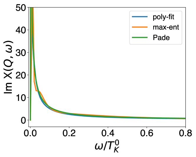
Figure S1: Comparison between the different methods of analytical continuation.   The blue, orange and green curves correspond to ${\it Im}\chi(\bm{Q},\omega)$ at $T/T_{K}^{0}=2.5\times 10^{-3}$ obtained from the polynomial fitting, maximal entropy method and Padé decomposition, respectively.

References

- 1 Bell, J. S. Speakable and unspeakable in quantum mechanics: Collected papers on quantum philosophy (Cambridge university press, 2004). URL https://doi.org/10.1017/CBO9780511815676.
- 2 Nielsen, M. A. & Chuang, I. L. Quantum computation and quantum information (Cambridge university press, 2010). URL https://doi.org/10.1017/CBO9780511976667.
- 3 Coffman, V., Kundu, J. & Wootters, W. K. Distributed entanglement. Physical Review A 61, 052306 (2000). URL https://link.aps.org/doi/10.1103/PhysRevA.61.052306.
- 4 Vidal, G., Latorre, J. I., Rico, E. & Kitaev, A. Entanglement in quantum critical phenomena. Physical Review Letters 90, 227902 (2003). URL https://link.aps.org/doi/10.1103/PhysRevLett.90.227902.
- 5 Wen, X.-G. Quantum field theory of many-body systems: from the origin of sound to an origin of light and electrons (OUP Oxford, 2004). URL https://doi.org/10.1093/acprof:oso/9780199227259.001.0001.
- 6 Kitaev, A. & Preskill, J. Topological entanglement entropy. Physical Review Letters 96, 110404 (2006). URL https://link.aps.org/doi/10.1103/PhysRevLett.96.110404.
- 7 Li, H. & Haldane, F. D. M. Entanglement spectrum as a generalization of entanglement entropy: Identification of topological order in non-abelian fractional quantum hall effect states. Physical Review Letters 101, 010504 (2008). URL https://link.aps.org/doi/10.1103/PhysRevLett.101.010504.
- 8 Coleman, P. & Schofield, A. J. Quantum criticality. Nature 433, 226–229 (2005). URL https://doi.org/10.1038/nature03279.
- 9 Paschen, S. & Si, Q. Quantum phases driven by strong correlations. Nature Reviews Physics 3, 9–26 (2021). URL https://doi.org/10.1038/s42254-020-00262-6.
- 10 Prochaska, L., Li, X., MacFarland, D. C., Andrews, A. M., Bonta, M., Bianco, E. F., Yazdi, S., Schrenk, W., Detz, H., Limbeck, A., Si, Q., Ringe, E., Strasser, G., Kono, J. & Paschen, S. Singular charge fluctuations at a magnetic quantum critical point. Science 367, 285–288 (2020). URL https://www.science.org/doi/abs/10.1126/science.aag1595.
- 11 Cai, A., Yu, Z., Hu, H., Kirchner, S. & Si, Q. Dynamical scaling of charge and spin responses at a kondo destruction quantum critical point. Physical Review Letters 124, 027205 (2020). URL https://link.aps.org/doi/10.1103/PhysRevLett.124.027205.
- 12 Checkelsky, J. G., Bernevig, B. A., Coleman, P., Si, Q. & Paschen, S. Flat bands, strange metals and the kondo effect. Nature Reviews Materials (2024). URL https://doi.org/10.1038/s41578-023-00644-z.
- 13 Si, Q., Rabello, S., Ingersent, K. & Smith, J. L. Locally critical quantum phase transitions in strongly correlated metals. Nature 413, 804–808 (2001). URL https://doi.org/10.1038/35101507.
- 14 Coleman, P., Pépin, C., Si, Q. & Ramazashvili, R. How do fermi liquids get heavy and die? Journal of Physics: Condensed Matter 13, R723 (2001). URL https://dx.doi.org/10.1088/0953-8984/13/35/202.
- 15 Senthil, T., Vojta, M. & Sachdev, S. Weak magnetism and non-fermi liquids near heavy-fermion critical points. Physical Review B 69, 035111 (2004). URL https://link.aps.org/doi/10.1103/PhysRevB.69.035111.
- 16 Islam, R., Ma, R., Preiss, P. M., Eric Tai, M., Lukin, A., Rispoli, M. & Greiner, M. Measuring entanglement entropy in a quantum many-body system. Nature 528, 77–83 (2015). URL https://doi.org/10.1038/nature15750.
- 17 Klich, I. & Levitov, L. Quantum noise as an entanglement meter. Physical Review Letters 102, 100502 (2009). URL https://link.aps.org/doi/10.1103/PhysRevLett.102.100502.
- 18 Hyllus, P., Laskowski, W., Krischek, R., Schwemmer, C., Wieczorek, W., Weinfurter, H., Pezzé, L. & Smerzi, A. Fisher information and multiparticle entanglement. Physical Review A 85, 022321 (2012). URL https://link.aps.org/doi/10.1103/PhysRevA.85.022321.
- 19 Liu, J., Yuan, H., Lu, X.-M. & Wang, X. Quantum fisher information matrix and multiparameter estimation. Journal of Physics A: Mathematical and Theoretical 53, 023001 (2019). URL https://dx.doi.org/10.1088/1751-8121/ab5d4d.
- 20 Hauke, P., Heyl, M., Tagliacozzo, L. & Zoller, P. Measuring multipartite entanglement through dynamic susceptibilities. Nature Physics 12, 778–782 (2016). URL https://www.nature.com/articles/nphys3700.
- 21 Laurell, P., Scheie, A., Mukherjee, C. J., Koza, M. M., Enderle, M., Tylczynski, Z., Okamoto, S., Coldea, R., Tennant, D. A. & Alvarez, G. Quantifying and controlling entanglement in the quantum magnet . Phys. Rev. Lett. 127, 037201 (2021). URL https://link.aps.org/doi/10.1103/PhysRevLett.127.037201.
- 22 Scheie, A. O., Ghioldi, E. A., Xing, J., Paddison, J. A. M., Sherman, N. E., Dupont, M., Sanjeewa, L. D., Lee, S., Woods, A. J., Abernathy, D., Pajerowski, D. M., Williams, T. J., Zhang, S.-S., Manuel, L. O., Trumper, A. E., Pemmaraju, C. D., Sefat, A. S., Parker, D. S., Devereaux, T. P., Movshovich, R., Moore, J. E., Batista, C. D. & Tennant, D. A. Proximate spin liquid and fractionalization in the triangular antiferromagnet KYbSe2. Nature Physics 20, 74–81 (2024). URL https://doi.org/10.1038/s41567-023-02259-1.
- 23 Scheie, A., Laurell, P., Samarakoon, A. M., Lake, B., Nagler, S. E., Granroth, G. E., Okamoto, S., Alvarez, G. & Tennant, D. A. Witnessing entanglement in quantum magnets using neutron scattering. Physical Review B 103, 224434 (2021). URL https://link.aps.org/doi/10.1103/PhysRevB.103.224434.
- 24 Hales, J., Bajpai, U., Liu, T., Baykusheva, D. R., Li, M., Mitrano, M. & Wang, Y. Witnessing light-driven entanglement using time-resolved resonant inelastic x-ray scattering. Nature Communications 14, 3512 (2023). URL https://doi.org/10.1038/s41467-023-38540-3.
- 25 Malla, R. K., Weichselbaum, A., Wei, T.-C. & Konik, R. M. Detecting Multipartite Entanglement Patterns using Single Particle Green’s Functions. arXiv e-prints arXiv:2310.05870 (2023). URL https://doi.org/10.48550/arXiv.2310.05870. eprint 2310.05870.
- 26 Hewson, A. C. The Kondo problem to heavy fermions (Cambridge university press, 1997). URL https://doi.org/10.1017/CBO9780511470752.
- 27 Kirchner, S., Paschen, S., Chen, Q., Wirth, S., Feng, D., Thompson, J. D. & Si, Q. Colloquium: Heavy-electron quantum criticality and single-particle spectroscopy. Reviews of Modern Physics 92, 011002 (2020). URL https://link.aps.org/doi/10.1103/RevModPhys.92.011002.
- 28 Pixley, J. H., Chowdhury, T., Miecnikowski, M. T., Stephens, J., Wagner, C. & Ingersent, K. Entanglement entropy near kondo-destruction quantum critical points. Physical Review B 91, 245122 (2015). URL https://link.aps.org/doi/10.1103/PhysRevB.91.245122.
- 29 Wagner, C., Chowdhury, T., Pixley, J. H. & Ingersent, K. Long-range entanglement near a kondo-destruction quantum critical point. Physical Review Letters 121, 147602 (2018). URL https://link.aps.org/doi/10.1103/PhysRevLett.121.147602.
- 30 Bayat, A., Bose, S., Sodano, P. & Johannesson, H. Entanglement probe of two-impurity kondo physics in a spin chain. Physical Review Letters 109, 066403 (2012). URL https://link.aps.org/doi/10.1103/PhysRevLett.109.066403.
- 31 Bayat, A., Sodano, P. & Bose, S. Negativity as the entanglement measure to probe the kondo regime in the spin-chain kondo model. Physical Review B 81, 064429 (2010). URL https://link.aps.org/doi/10.1103/PhysRevB.81.064429.
- 32 Alkurtass, B., Bayat, A., Affleck, I., Bose, S., Johannesson, H., Sodano, P., Sørensen, E. S. & Le Hur, K. Entanglement structure of the two-channel kondo model. Physical Review B 93, 081106 (2016). URL https://link.aps.org/doi/10.1103/PhysRevB.93.081106.
- 33 Parisen Toldin, F., Sato, T. & Assaad, F. F. Mutual information in heavy-fermion systems. Physical Review B 99, 155158 (2019). URL https://link.aps.org/doi/10.1103/PhysRevB.99.155158.
- 34 Hu, H., Cai, A. & Si, Q. Quantum Criticality and Dynamical Kondo Effect in an SU(2) Anderson Lattice Model. arXiv e-prints arXiv:2004.04679 (2020). URL https://doi.org/10.48550/arXiv.2004.04679. eprint 2004.04679.
- 35 Wootters, W. K. Entanglement of formation of an arbitrary state of two qubits. Physical Review Letters 80, 2245–2248 (1998). URL https://link.aps.org/doi/10.1103/PhysRevLett.80.2245.
- 36 Amico, L., Osterloh, A., Plastina, F., Fazio, R. & Massimo Palma, G. Dynamics of entanglement in one-dimensional spin systems. Physical Review A 69, 022304 (2004). URL https://link.aps.org/doi/10.1103/PhysRevA.69.022304.
- 37 Osborne, T. J. & Verstraete, F. General monogamy inequality for bipartite qubit entanglement. Physical Review Letters 96, 220503 (2006). URL https://link.aps.org/doi/10.1103/PhysRevLett.96.220503.
- 38 Hu, H., Chen, L. & Si, Q. Extended Dynamical Mean Field Theory for Correlated Electron Models. arXiv e-prints arXiv:2210.14197 (2022). URL https://doi.org/10.48550/arXiv.2210.14197. eprint 2210.14197.
- 39 Si, Q. & Smith, J. L. Kosterlitz-thouless transition and short range spatial correlations in an extended hubbard model. Physical Review Letters 77, 3391–3394 (1996). URL https://link.aps.org/doi/10.1103/PhysRevLett.77.3391.
- 40 Smith, J. L. & Si, Q. Spatial correlations in dynamical mean-field theory. Physical Review B 61, 5184–5193 (2000). URL https://link.aps.org/doi/10.1103/PhysRevB.61.5184.
- 41 Chitra, R. & Kotliar, G. Effect of long range coulomb interactions on the mott transition. Physical Review Letters 84, 3678–3681 (2000). URL https://link.aps.org/doi/10.1103/PhysRevLett.84.3678.
- 42 Hu, H., Chen, L. & Si, Q. Quantum Critical Metals: Dynamical Planckian Scaling and Loss of Quasiparticles. arXiv e-prints arXiv:2210.14183 (2022). URL https://doi.org/10.48550/arXiv.2210.14183. eprint 2210.14183.
- 43 Helstrom, C. W. Quantum detection and estimation theory. Journal of Statistical Physics 1, 231–252 (1969). URL https://doi.org/10.1007/BF01007479.
- 44 Holevo, A. S. Probabilistic and statistical aspects of quantum theory, vol. 1 (Springer Science & Business Media, 2011). URL https://doi.org/10.1007/978-88-7642-378-9.
- 45 Kay, S. M. Fundamentals of statistical signal processing: estimation theory (Prentice-Hall, Inc., 1993). URL https://dl.acm.org/doi/10.5555/151045.
- 46 Pezzè, L., Smerzi, A., Oberthaler, M. K., Schmied, R. & Treutlein, P. Quantum metrology with nonclassical states of atomic ensembles. Reviews of Modern Physics 90, 035005 (2018). URL https://link.aps.org/doi/10.1103/RevModPhys.90.035005.
- 47 Braunstein, S. L. & Caves, C. M. Statistical distance and the geometry of quantum states. Physical Review Letters 72, 3439–3443 (1994). URL https://link.aps.org/doi/10.1103/PhysRevLett.72.3439.
- 48 Braunstein, S. L., Caves, C. M. & Milburn, G. Generalized uncertainty relations: Theory, examples, and lorentz invariance. Annals of Physics 247, 135–173 (1996). URL https://www.sciencedirect.com/science/article/pii/S0003491696900408.
- 49 Petz, D. & Ghinea, C. Introduction to Quantum Fisher Information. In Rebolledo, R. & Orszag, M. (eds.) Quantum Probability and Related Topics, 261–281 (2011). URL https://doi.org/10.1142/9789814338745_0015. eprint 1008.2417.
- 50 Tóth, G., Moroder, T. & Gühne, O. Evaluating convex roof entanglement measures. Physical Review Letters 114, 160501 (2015). URL https://link.aps.org/doi/10.1103/PhysRevLett.114.160501.