Probabilistic work extraction on a classical oscillator beyond the second law

Abstract

We demonstrate experimentally that, applying optimal protocols which drive the system between two equilibrium states characterized by a free energy difference $\Delta F$, we can maximize the probability of performing the transition between the two states with a work $W$ smaller than $\Delta F$. The second law holds only on average, resulting in the inequality $\langle W\rangle\geq\Delta F$. The experiment is performed using an underdamped oscillator evolving in a double-well potential. We show that with a suitable choice of parameters the probability of obtaining trajectories with $W\leq\Delta F$ can be larger than $90\,\%$. Very fast protocols are a key feature to obtain these results which are explained in terms of the Jarzynski equality.

I Introduction

Numerous experimental platforms that act on the micro and nano scales allow us to explore the laws of thermodynamics for systems with few degrees of freedom coupled with thermal baths [1]. Typical examples are experiments in colloids [2, 3, 4, 5, 6, 7], electric circuits [8], single electron transistors [9, 10], mechanical devices [11, 12] and single molecules [13, 14]. In such systems, fluctuations of physical quantities play a fundamental role, contrary to classical thermodynamics which mostly considers averaged quantities. Stochastic thermodynamics provides the suited framework to describe single realizations of thermodynamic transformation, and the associated work and heat distribution. In particular, the second law does not apply at the level of a single realization, and one can observe local “violations” due to the stochastic nature of the system, where the system can extract work, or gain free energy, at no cost to the operator and with no information feedback (illustration in Fig. 1) [15, 16, 17, 18].

In a system driven by an external control parameter $\lambda$ from an initial to a final equilibrium state resulting in a free energy difference $\Delta F$ between the two states, the probability distribution of the work performed when changing $\lambda$ is constrained by Jarzynski’s equality [19]

$$\langle\mathrm{e}^{-\beta W}\rangle=\mathrm{e}^{-\beta\Delta F},$$ (1)

where $\beta=1/k_{B}T$, with $T$ the temperature of the system and $k_{B}$ the Boltzmann constant. The expression of the second law can be recovered from the convexity of the exponential function: $\langle W\rangle\geq\Delta F$. We are interested here in realizations where the free energy of the system can be increased spending an amount of work $W<\Delta F$. The free energy stored in the system can be later used, resulting in probabilistic work extraction from the device.

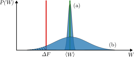
Figure 1: Probability distribution function of the work $P(W)$ during a transformation. (a) In classical macroscopic thermodynamics, fluctuations are usually negligible compared with the mean value. (b) However, in stochastic thermodynamics, such fluctuations can lead to local “violations” of the second law: several realisations of a transformation can be performed with a work $W$ smaller than the free energy difference $\Delta F$ (hatched area), even if in average $\langle W\rangle\geq\Delta F$. Note that in this sketch, the horizontal axis is rescaled between (a) and (b).

These realizations have been theoretically [10] and experimentally studied [9] with a single electron transistor with discrete energy levels, obtaining a probability of extracting work up to $65\text{\,}\%$. Using a mechanical oscillator, we want to illustrate this behavior using a fully classical continuous system. Our goal is to experimentally obtain an arbitrary large probability of having realizations with $W<\Delta F$. Also, we approach the optimal work distribution predicted by [10] to observe such events at a fixed mean cost of energy.

II Experimental setup and protocol

The experimental setup is a microcantilever, which behaves in the absence of external forces as an underdamped harmonic oscillator of stiffness $k$, resonance frequency $f_{0}=1200Hz$ and quality factor $Q=10$. The deflection $x$ of the cantilever is measured by interferometry [20]. The oscillator is in equilibrium with the surrounding air at room temperature $T$ and subject to thermal fluctuations. The variance of $x$ is $\sigma^{2}=\langle x^{2}\rangle=k_{B}T/k\sim$1\text{\,}\mathrm{n}\mathrm{m}^{2}$$. $\sigma$ is used as the unit length, and from now on all positions are expressed as dimensionless quantities $z=x/\sigma$, and energies in units of $k_{B}T$ (hence taking $\beta=1$ in Jarzynski’s equality, Eq. 1).

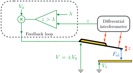
Figure 2: Sketch of the experimental setup. We record the deflection $z$ of a conductive cantilever measured with high precision by a differential interferometer [20]. Depending on the comparison of $z$ to a tunable threshold $\lambda$, a constant voltage $V=\pm V_{0}$ is applied by a fast feedback loop, creating an electrostatic force $F_{\mathrm{el}}$ on the cantilever towards a nearby electrode at voltage $V_{1}\gg V_{0}$.

To tune the potential experienced by the resonator, we use an electrostatic force acting on the cantilever. A time-dependent virtual potential can be created by a fast feedback loop [11, 21] that adjusts the voltage $V$ applied to the cantilever (thus the electrostatic force) depending on the measured position $z$ (see Fig. 2). We implement the following simple rule: $V=-V_{0}$ if the position is below a threshold $\lambda$, and $V=+V_{0}$ otherwise. This creates an asymmetric double well, illustrated in Fig. 3. Two parameters are available to tune the potential: $\lambda$ sets the barrier position and $V_{0}$ sets the centers of the two wells in $\pm z_{0}\propto\pm V_{0}$.

Theoretically, the potential energy constructed by this feedback is:

$$\begin{split}U(z,\lambda,z_{0})=&\frac{1}{2}\big{(}z-S(z-\lambda)z_{0}\big{)}^{2}\\ &+\lambda z_{0}\big{(}S(z-\lambda)+S(\lambda)\big{)},\end{split}$$ (2)

where $S$ is the sign function: $S(z-\lambda)=-1$ if $z<\lambda$ and $S(z-\lambda)=1$ if $z>\lambda$. To illustrate the validity of this model for $U$, we record a long time trace of the position in a static potential to evaluate the probability distribution function (pdf) of the position $P(z)$. We then reconstruct the double well using Boltzmann’s prescription at equilibrium:

$$P(z) =\frac{1}{Z(\lambda,z_{0})}\mathrm{e}^{-U(z,\lambda,z_{0})},$$ (3a)

$$Z(\lambda,z_{0}) =\int_{-\infty}^{+\infty}\mathrm{e}^{-U(z,\lambda,z_{0})}\mathrm{d}z,$$ (3b)

with $Z$ the partition function. As plotted in Fig. 3, the model is an excellent description of the effective potential evaluated through $U(z)=-\ln[P(z)/P(-S(\lambda)z_{0})]$.

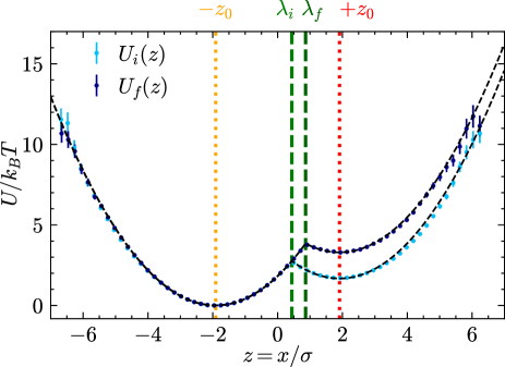
Figure 3: Double well potentials. The potential energy of the cantilever is the juxtaposition of two harmonic wells centered in $\pm z_{0}=\pm 1.91$, the switch between the two occurring when $z=\lambda$. The two examples plotted here correspond to $\lambda_{i}=0.44$ and $\lambda_{f}=0.86$. The measured potential $U(z)$ data is inferred from Eq. 3 and the pdf of the experimental positions $z$ during a long acquisition. The black dashed lines are best fit to Eq. 2, leading to the aforementioned values of $z_{0}$ and $\lambda$. The transformation we apply corresponds to a step of $\lambda$ from $\lambda_{i}$ to $\lambda_{f}$, leaving the lower well untouched while raising the upper one by $\Delta U=2(\lambda_{f}-\lambda_{i})x_{0}$.

To observe local “violations” of the second law, we design the following protocol between an initial state (all quantities labeled by the subscript _i) and a final state (subscript _f). First, the cantilever evolves at equilibrium in an initial double-well potential $U_{i}(z)=U(z,\lambda_{i},z_{0})$. Then, we instantaneously increase the threshold $\lambda$ between the two wells, from $\lambda_{i}$ to $\lambda_{f}$. Finally, the cantilever is left in the final potential $U_{f}(z)=U(z,\lambda_{f},z_{0})$. The well centers are left unchanged during the protocol, $z_{0}$ keeping the same value. An example of the time trace of one realisation of such protocol is plotted in Fig. 4.

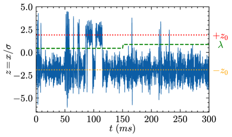
Figure 4: Trajectory of an underdamped oscillator evolving in a time-dependent asymmetric double-well potential. The position $z$ is expressed in units of standard deviation $\sigma$ in a single well. The center of the wells is kept constant at $\pm z_{0}=\pm 1.91$, but the commutation threshold $\lambda$ is changed from $\lambda_{i}=0.44$ to $\lambda_{f}=0.86$ at $t=$150\text{\,}\mathrm{m}\mathrm{s}$$.

Initial and final potentials are represented in Fig. 3. Each potential is measured from the equilibrium pdf $P(z)$ in the initial and final state, then fitted with very good accuracy using Eq. 2. The experimental values of the parameters $\lambda_{i}$, $\lambda_{f}$ and $z_{0}$ are deduced from the fit. Potential wise, the protocol amounts to leaving the lower well unaffected while raising the upper one. The work $W$ performed will be $0$ most of the time (anytime the system is in the lower well, which is likely), while the free energy difference is positive (since $U(x)$ is globally increasing): the probability of observing $W<\Delta F$ should thus be high.

The values of $z_{0}=1.91$ and $\lambda_{f}=0.86$ are the same for all experiments. We tune the initial threshold $\lambda_{i}$ with values going from 0 to 0.75. For each one of them, the protocol detailed in Fig. 4 is repeated around $N\sim 1000$ times. This allows us to obtain a good enough statistics to estimate the pdf $P(z)$, and further on the work distribution.

III Analysis

Following the classical convention of stochastic thermodynamics [16], we define the work $W$ done by the operator through the variations of the external parameters tuning the potential $U(z,\lambda,z_{0})$:

$$W=\int\frac{\partial U}{\partial\lambda}\dot{\lambda}\mathrm{d}t.$$ (4)

Since $z_{0}$ is kept constant in all protocols, we do not consider the term in $\dot{z}_{0}$ which is always zero here. $W$ is computed using the recorded trajectories $z(t)$ and Eq. 2. Since the variation of $\lambda(t)$ is a step function, the work can be equivalently computed as $W=U_{f}(z)-U_{i}(z)$ using the value of $z$ at the moment of the switch. From this expression we can also infer the theoretical expectation for $\langle W\rangle$:

$$\langle W\rangle =\int_{-\infty}^{+\infty}\big{[}U_{f}(z)-U_{i}(z)\big{]}\frac{1}{Z_{i}}\mathrm{e}^{-U_{i}(z)}\mathrm{d}z,$$ (5a)

$$=\frac{2z_{0}\mathrm{e}^{-2\lambda_{i}z_{0}}}{Z_{i}}\big{[}f(\lambda_{f}-z_{0})-f(\lambda_{i}-z_{0})\big{]},$$ (5b)

where $f$ is defined by

$$f(u)=\sqrt{\pi/2}\,u\,\mathrm{erfc}\left(-u/\sqrt{2}\right)-\mathrm{e}^{-u^{2}/2}.$$ (6)

$Z_{i}=Z(\lambda_{i},z_{0})$ is the partition function in the initial state, which can be computed from Eq. 3b as:

$$\begin{split}Z(\lambda,z_{0})=\sqrt{\frac{\pi}{2}}\bigg{[}2&-\mathrm{erfc}\bigg{(}\frac{\lambda+z_{0}}{\sqrt{2}}\bigg{)}\\ &+\mathrm{e}^{-2\lambda z_{0}}\mathrm{erfc}\bigg{(}\frac{\lambda-z_{0}}{\sqrt{2}}\bigg{)}\bigg{]}.\end{split}$$ (7)

The free energy difference in the system $\Delta F=F_{f}-F_{i}$ can be computed in two different ways. For a given protocol, the work distribution obeys Jarzynski’s equality (Eq. 1), thus $\Delta F=-\ln\langle e^{-W}\rangle$ can be deduced from the experimental work distribution with good enough statistics. The second approach is to use the partition function $Z$ at equilibrium: since the free energy of the system is $F=-\ln(Z)$, the free energy difference $\Delta F=\ln(Z_{i}/Z_{f})$ can be theoretically directly calculated from the parameters of the initial and final potentials.

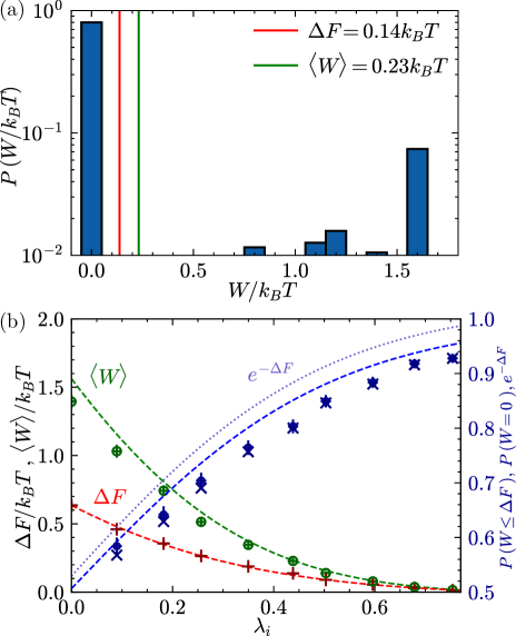
Figure 5: (a) Work distribution for $N=968$ protocols, corresponding to the protocol in Fig. 3 ($\lambda_{i}=0.44$, $\lambda_{f}=0.86$). We also report the mean work $\langle W\rangle=0.23\pm 0.02$ and free energy difference $\Delta F=0.14\pm 0.01$ computed using Jarzynski’s equality. We observe a transient violation of the second law in more than 80% of the protocols (note the vertical log scale). (b) Mean work $\langle W\rangle$ ($\circ$, top curve) and free energy difference $\Delta F$ ($+$, bottom curve) and for all initial conditions $\lambda_{i}$. Experiment (markers with error bars corresponding to one standard deviation of the statistical uncertainties) and theory (dashed lines) are in good agreement. The second law of thermodynamics $\langle W\rangle\geq\Delta F$ always holds, though the probability of observing the contrary on the single trajectory reaches over $90\text{\,}\%$ for the highest values of $\lambda_{i}$ ($\circ$ marker, experiment, and dashed blue line, theory, right vertical scale). The probability of observing a zero work $P(W=0)$ ($\times$) almost coincide with the one of transiently violating the second law, and is upper bounded by $\mathrm{e}^{-\Delta F}$ (dotted blue line, right vertical scale), as predicted by Eq. 10 [22].

IV Results

The protocol is repeated $N\sim 1000$ times for 10 values of $\lambda_{i}$ ranging from 0 to 0.75. For each $\lambda_{i}$, we compute the work distribution. An example for $\lambda_{i}=0.44$ is plotted in Fig. 5(a), where we also report the mean work $\langle W\rangle$ performed by the driving, and the difference in free energy $\Delta F$. The work distribution consists mostly of two narrow peaks. The first one, for $W=0$, corresponds to the cases where the cantilever was in the lower well ($z<\lambda_{i}$) of the potential during the step of $\lambda$. Since there is no change in the lower part of the potential, there is no energy cost. The second peak comes from the cases where $z>\lambda_{f}$: in this area, the potential is shifted by $\Delta U=2z_{0}(\lambda_{f}-\lambda_{i})$, and driving the parameter $\lambda$ implies this amount of work. We also observe some intermediate values, corresponding to $\lambda_{i}<z<\lambda_{f}$: the cantilever is initially in the upper well but ends in the lower one due to the step in in $\lambda$, resulting in an intermediate energy change $\Delta U=2z_{0}(z-\lambda_{i})$, where $z$ is the value of the deflection at the time of the switch.

As illustrated in Fig. 5(b), the second law is always satisfied ($\langle W\rangle>\Delta F$), but we manage to observe an almost arbitrary large proportion of transient violations ($W<\Delta F$). Indeed, by tuning the initial asymmetry of the potential, we can increase the probability of being in the lower well ($z<\lambda_{i}$) during the switch. The probability of observing a transient violation of the second law $P(W<\Delta F)$ can thus be arbitrary large. With our choice of parameters, for values of $\lambda_{i}$ very close to the final value of $\lambda_{f}$, we manage to measure values of $P(W<\Delta F)$ greater than 90% . Our experimental results are very close to the theoretical expectation:

$$\!\!P(W<\Delta F) =\int_{0}^{\Delta F}P(W)\mathrm{d}W=\int_{-\infty}^{\lambda_{i}+\Delta F/(2z_{0})}\frac{1}{Z_{i}}\mathrm{e}^{-U_{i}(z)}\mathrm{d}z$$ (8)

$$=\frac{1}{Z(\lambda_{i},z_{0})}\sqrt{\frac{\pi}{2}}\bigg{[}2-\mathrm{erfc}\bigg{(}\frac{\lambda_{i}+z_{0}}{\sqrt{2}}\bigg{)}+\mathrm{e}^{-2\lambda_{i}z_{0}}\mathrm{erfc}\bigg{(}\frac{\lambda_{i}-z_{0}}{\sqrt{2}}\bigg{)}-\mathrm{e}^{-2\lambda_{i}z_{0}}\mathrm{erfc}\bigg{(}\frac{\Delta F/(2z_{0})+\lambda_{i}-z_{0}}{\sqrt{2}}\bigg{)}\bigg{]}.$$ (9)

However, the free energy $\Delta F$ decreases when increasing $\lambda_{i}$: work extraction is more and more likely, but the gain with respect to $\Delta F$ decreases.

Another theoretical result that we can probe with our experiment is the inequality [22]:

$$P(W\leq 0)\leq\mathrm{e}^{-\Delta F}.$$ (10)

In our case, $P(W\leq 0)=P(W=0)$ since $W$ cannot be negative. Moreover, this probability is very close to $P(W\leq\Delta F)$ since the work distribution consists mainly of two peaks: one in $0$ and the other above $\Delta F$. In the experiments, the two probabilities coincide within statistical uncertainties, as shown in Fig. 5(b). In this same figure, we plot the upper bound given by Eq. 10, which is indeed confirmed in our experiment, and close to be saturated.

Conclusion

We have shown, using a fully classical continuous mechanical system, how we can observe an arbitrary large number of apparent “violations” of the second law of thermodynamics, while being consistent with the rules of stochastic thermodynamics. We show a clear trade-off between this probability and the free energy gained during those events. We almost reach the theoretical limit of $95\%$ probability (for our set of parameters) of having anomalous trajectories with $W<\Delta F$. This result is made possible by the specific way in which the potential is changed during the protocol. Indeed the stiffness of the two wells does not change and only the minimum of the upper well is raised. This protocol produces a work probability distribution with mainly two Dirac functions that matches the optimal distribution described in Ref. [10] to maximize the work extraction probability. One Dirac peak is centered in zero and corresponds to the trajectories that start in the lower well. The other is centered to a positive value of the work and corresponds to the trajectories starting on the upper well. In our experiment the relative amplitude of the two peaks, which determines the amount of “anomalous” trajectories, can be tuned by changing the minimum positions of the wells through the value of $\lambda$. In this way we have transformed for the transition properties a continuous classical system to a two levels system, showing similarities with the one of ref. [9]. In this context, the fast switch between the initial and final state is a key ingredient of the protocol, again as proposed in Ref. [10]. Indeed a slow ramp would broaden the peaks of the work distribution, resulting in a situation similar to Fig. 1(b). For such symmetric distributions, where the mean and the median are equal, observing $W<\Delta F$ is unlikely: the probability is smaller than $50\text{\,}\%$, this limit being reached in the reversible limit. Let us to conclude by saying that in spite of the fact there is an energy gain for $90\%$ of the trajectories, the total mean remains positive and in order to use this energy surplus one should introduce a demon which selects the good trajectories, i.e. those starting on the lower well.

References

- Ciliberto [2017] S. Ciliberto, Experiments in stochastic thermodynamics: Short history and perspectives, Phys. Rev. X 7, 021051 (2017).
- Blickle et al. [2006] V. Blickle, T. Speck, L. Helden, U. Seifert, and C. Bechinger, Thermodynamics of a colloidal particle in a time-dependent nonharmonic potential, Phys. Rev. Lett. 96, 070603 (2006).
- Gavrilov and Bechhoefer [2016] M. Gavrilov and J. Bechhoefer, Erasure without work in an asymmetric, double-well potential, Phys. Rev. Lett. 117, 200601 (2016).
- Bérut et al. [2012] A. Bérut, A. Arakelyan, A. Petrosyan, S. Ciliberto, R. Dillenschneider, and E. Lutz, Experimental verification of Landauer’s principle linking information and thermodynamics, Nature 483, 187 (2012).
- Martinez et al. [2015] I. Martinez, E. Roldán, L. Dinis, D. Petrov, and R. A. Rica, Adiabatic processes realized with a trapped brownian particle, Phys. Rev. Lett. 114, 120601 (2015).
- Jun et al. [2014] Y. Jun, M. Gavrilov, and J. Bechhoefer, High-precision test of landauer’s principle in a feedback trap, Phys. Rev. Lett. 113, 190601 (2014).
- Toyabe et al. [2010] S. Toyabe, T. Sagawa, M. Ueda, M. Muneyuki, and M. Sano, Experimental demonstration of information-to-energy conversion and validation of the generalized Jarzynski equality, Nat. Phys. 6, 988 (2010).
- Ciliberto et al. [2013] S. Ciliberto, A. Imparato, A. Naert, and M. Tanase, Heat flux and entropy produced by thermal fluctuations, Phys. Rev. Lett. 110, 180601 (2013).
- Maillet et al. [2019] O. Maillet, P. A. Erdman, V. Cavina, B. Bhandari, E. T. Mannila, J. T. Peltonen, A. Mari, F. Taddei, C. Jarzynski, V. Giovannetti, and J. P. Pekola, Optimal probabilistic work extraction beyond the free energy difference with a single-electron device, Phys. Rev. Lett. 122, 150604 (2019).
- Cavina et al. [2016] V. Cavina, A. Mari, and V. Giovannetti, Optimal processes for probabilistic work extraction beyond the second law, Sci. Rep. 6, 29282 (2016).
- Dago et al. [2022] S. Dago, J. Pereda, S. Ciliberto, and L. Bellon, Virtual double-well potential for an underdamped oscillator created by a feedback loop, J. Stat. Mech. 2022, 053209 (2022).
- Joubaud et al. [2007] S. Joubaud, B. Garnier, N., and S. Ciliberto, Fluctuation theorems for harmonic oscillators, J. Stat. Mech. , P09018 (2007).
- Collin et al. [2005] D. Collin, F. Ritort, C. Jarzynski, S. Smith, I. Tinoco, and C. Bustamante, Verification of the Crooks fluctuation theorem and recovery of RNA folding free energies, Nature 437, 231 (2005).
- Ribezzi-Crivellari and Ritort [2019] M. Ribezzi-Crivellari and F. Ritort, Large work extraction and the Landauer limit in a continuous Maxwell demon, Nat. Phys. 15, 660 (2019).
- Jarzynski [2011] C. Jarzynski, Equalities and inequalities: Irreversibility and the second law of thermodynamics at the nanoscale, Annu. Rev. Condens. Matter Phys. 2, 329 (2011).
- Sekimoto [2010] K. Sekimoto, Stochastic Energetics, Lect. Notes Phys., Vol. 799 (Springer, Berlin Heidelberg, 2010).
- Seifert [2012] U. Seifert, Stochastic thermodynamics, fluctuation theorems and molecular machines, Rep. Prog. Phys. 75, 126001 (2012).
- Sagawa [2014] T. Sagawa, Thermodynamic and logical reversibilities revisited, J. Stat. Mech. 2014, P03025 (2014).
- Jarzynski [1997] C. Jarzynski, Nonequilibrium equality for free energy differences, Phys. Rev. Lett. 78, 2690 (1997).
- Paolino et al. [2013] P. Paolino, F. Aguilar Sandoval, and L. Bellon, Quadrature phase interferometer for high resolution force spectroscopy, Rev. Sci. Instrum. 84, 095001 (2013).
- [21] S. Dago, N. Barros, J. Pereda, S. Ciliberto, and L. Bellon, Virtual potential created by a feedback loop: taming the feedback demon to explore stochastic thermodynamics of underdamped systems, arXiv: 2311.12687 (2023).
- Jarzynski [2008] C. Jarzynski, Nonequilibrium work relations: foundations and applications, Eur. Phys. J. B 64, 331 (2008).
- Barros et al. [2023] N. Barros, S. Ciliberto, and L. Bellon, Dataset: Probabilistic work extraction on a classical oscillator beyond the second law (2023), Zenodo. doi:10.5281/zenodo.10721407.