Generalised Hydrodynamics description of the Page curve-like dynamics of a freely expanding fermionic gas
Abstract
We consider an analytically tractable model that exhibits the main features of the Page curve characterizing the evolution of entanglement entropy during evaporation of a black hole. Our model is a gas of non-interacting fermions on a lattice that is released from a box into the vacuum. More precisely, our Hamiltonian is a tight-binding model with a defect at the junction between the filled box and the vacuum. In addition to the entanglement entropy we consider several other observables, such as the spatial density profile and current, and show that the semiclassical approach of generalized hydrodynamics provides a remarkably accurate description of the quantum dynamics including that of the entanglement entropy at all times. Our hydrodynamic results agree closely with those obtained via exact microscopic numerics. We find that the growth of entanglement is linear and universal, i.e, independent of the details of the defect. The decay shows scaling for conformal defect while for non-conformal defects, it is slower. Our study shows the power of the semiclassical approach and could be relevant for discussions on the resolution of the black hole information paradox.
Introduction— Entanglement is a quantity of immense interest Eisert et al. (2010); Nishioka (2018); Latorre and Riera (2009); Calabrese and Cardy (2009); Coppola et al. (2022); Liu and Vardhan (2021) spanning and connecting different areas such as quantum information, quantum many body physics, black hole physics to name a few. The entanglement entropy characterizes quantum correlations between two parts of a given system in a pure state and indicates how far it is from a product form. An interesting question is that of the time evolution of the entanglement entropy, in a many body system, between a subsystem and its complement. Concrete results were obtained by Calabrese and Cardy for one dimensional noninteracting systems using path integral methods and also explicit calculations on lattice models Calabrese and Cardy (2005, 2007, 2009). A number of subsequent papers have studied this problem for both interacting Alba et al. (2021); Alba and Calabrese (2017a); Eisler and Bauernfeind (2017); Žnidarič (2020) and non-interacting Bertini et al. (2018); Dubail et al. (2017); Fagotti and Calabrese (2010); Scopa et al. (2021); Eisler and Peschel (2010); Gamayun et al. (2020); Song et al. (2011); Ares et al. (2022); Eisler and Peschel (2012); Capizzi et al. (2023) one-dimensional integrable models and in general one finds that the entanglement entropy initially increases linearly with time (in some cases logarithmically) and eventually saturates to a value that is consistent with the volume law Ho and Abanin (2017); Kim and Huse (2013).
There is also a lot of interest in the setup where there is a possible decay in the entanglement entropy at late times. This is often described by the Page curve that is usually discussed in the context of the evaporation of a black hole. Page Page (1993, 2013) considered the entanglement between the black hole and the radiation starting from the unentangled initial state of just the black hole. As the black hole radiates, the effective Hilbert space dimension of the radiation increases and, assuming maximal entanglement, there will be a corresponding increase in the entanglement entropy. However, this increase has to stop at some time when the black hole and radiation have the same Hilbert space dimensions. Beyond this time (referred to as the Page time), the entropy has to decrease. This non-monotonic behavior was not captured in Hawking’s semiclassical calculation Hawking (1975) leading to the famous information paradox Almheiri et al. (2021); Raju (2022); Mathur (2009), see also Maes (2015) for a critique. In fact, such non-monotonic behavior is also typically not observed in non-equilibrium studies of quantum many-body systems after a quench (discussed above Calabrese and Cardy (2005, 2007)), where typically the two partitions are of comparable size Ho and Abanin (2017); Kim and Huse (2013), and the entropy increases monotonically and saturates.
In this work, we show that by considering a partition consisting of a finite system and an infinite environment, one observes all the essential features of the Page entanglement curve, in particular the initial linear growth and the eventual decay. In two recent papers, this Page curve time dynamics behaviour has been observed for open fermionic Kehrein (2023) and bosonic Glatthard (2024) systems. Note that this is distinct from works reproducing the page curve in various free theories where entanglement is studied as a function of subsystem fraction for fixed Gaussian states Yu et al. (2023); Bianchi et al. (2022, 2021); Bhattacharjee et al. (2021).
Our microscopic model is the same as studied in Ref. Kehrein, 2023, namely an expanding free fermionic gas. Our main finding is that the Page curve behavior of entanglement entropy for this system is very accurately described from the equations of semi-classical generalized hydrodynamics which can be solved exactly. Our exact solution of the hydrodynamic equations reveals interesting features of the Page curve decay and also allows us to obtain analytic forms for various physical observables such as density profiles and particle current. We verify our hydrodynamics results from exact numerical computations. Interestingly, we find that even the average particle current has hints of the full Page curve while the particle number fluctuation displays the full form of the Page curve. The entropy obtained from hydrodynamics, is usually referred to as the Yang-Yang entropy and is a “coarse grained entropy” that counts the number of microstates corresponding to a given phase-space density Alba et al. (2021) (see also Pandey et al. (2023)). Remarkably, we find that the Yang-Yang entropy evaluated for the system agrees with the microscopic entanglement entropy at all times, while the same computed for its complement (the reservoir) differs from the entanglement entropy after around the Page time and keeps increasing.
Model— We consider the set up as shown in Fig. (1). The Hamiltonian for the full non-interacting set up can be written as,
| (1) |
Here, is the fermionic annihilation (creation) operator at site of the 1D chain. is the single particle Hamiltonian with . Here, is the nearest neighbor hopping strength except at the coupling between the finite system () and the semi-infinite reservoir (). For conformal defect, the coupling matrix elements are given as,
| (2) |
For other non-conformal defects such as hopping defect and density impurity, the coupling matrix elements of the Hamiltonian are given as,
| (3) | ||||
In the limit , the problem reduces to scattering of plane waves with wave-vector across the defect with transmission probability and reflection probability given by Ljubotina et al. (2019):
| (4) | ||||
Here, . For conformal defect, and ’s are independent and for non-conformal defect and ’s are dependent. Throghout the manuscript, we consider .

Exact calculations for microscopic entanglement entropy— To do the exact numerical calculations, we have to deal with finite-dimensional matrices. Thus, we write the finite dimensional form of the Hamiltonian in Eq. (1):
| (5) |
where is the length of the reservoir and we take . Here is a column vector containing all the annihilation operators. Similarly, is the row vector containing all the creation operators. The correlation matrix for any time can be written as,
| (6) |
Here, symbol is used for the transpose of the matrix. are the matrix elements of correlation matrix . Using the Heisenberg equation of motion, can be written as,
| (7) |
Here, is the initial correlation matrix. For this work, we consider the initial condition as filled finite system and empty large (infinite) system i.e. and otherwise . Thus the knowledge of the single particle spectrum of enables us to compute exactly the correlation matrix . Once we know from Eq. (7), we can evaluate all the physical observables like average current, density, entanglement entropy etc. The average current flowing from the system to the reservoir can be calculated using the elements of as,
| (8) |
The average density at any site and any time is the diagonal elements of i.e.
| (9) |
The entanglement entropy between the system and reservoir can be simply obtained Peschel and Eisler (2009) in terms of the eigenvalues of the correlation matrix, , which has the same elements as , but restricted to the range . In terms of the eigenvalues, , of , the von Neumann entropy is given by
| (10) |
Particle number fluctuations and entanglement entropy— It has been shown that the entanglement entropy is directly related to charge statistics in a quantum point contact set up as Klich and Levitov (2009); Gamayun et al. (2020); Song et al. (2011),
| (11) |
where are the cumulants corresponding to particle number fluctuations in the system and are Bernoulli numbers.
Thus, the major contribution to the entropy comes from the second cumulant which, in terms of eigenvalues of , can be written as Eisler and Rácz (2013),
| (12) |
Next, we will see, how using the generalized hydrodynamic description, we can calculate the quantities like average current, density and hydrodynamic entanglement entropy for this set up. Note that, the particle number fluctuation () has been computed Gamayun et al. (2020) from hydrodynamics for the case of infinite but we are not aware of results for finite .
Hydrodynamic description— The evolution of integrable systems observed on large time and length scales is described by generalized hydrodynamics Castro-Alvaredo et al. (2016); Bertini et al. (2016); Doyon (2020); Bertini et al. (2018); Essler (2022) which views the system as a gas of quasiparticles which carry fixed momentum labels and have a phase space density , with . For non-interacting systems such as the system of free fermions considered here, the quasiparticle velocities are given by , and the evolution of is given by the Euler equation,
| (13) |
This equation has to be solved with appropriate boundary conditions, which for our set-up are: (a) left-moving quasiparticles are reflected at the boundary (as ); (b) at the defect, right-moving quasiparticles inside the system are reflected (transmitted) with probability (, given by Eqs. (4). In terms of the quasiparticle distribution, physical observables such as the density profile and the hydrodynamic entropy density are given by
| (14) | ||||
| (15) |
This is the thermodynamic entropy density and also referred to as the Yang-Yang entropy Alba and Calabrese (2017b); Bertini et al. (2022). The system and reservoir entropies are then given by,
| (16) | ||||
| (17) |
Unlike for the case of domain wall initial conditions studied earlier in the literature Capizzi et al. (2023), our set up lacks particle-hole symmetry which means that and are not equal at all times. As we will see, it is that in fact gives precisely the entanglement entropy. Other observables, such as the total particle number in the system is simply given by , while the current into the reservoir is .
We now proceed to obtain a solution of Eq. (13) with the boundary conditions at the bounding wall at and at the defect at . We first note that the solution on the infinite line is given by
| (18) |
Here the initial phase space density, corresponding to the fully filled lattice is given by
| (19) |
In the presence of the defect at , the phase space density for is the sum of contributions where the final momentum of the quasi-particles is . Such contributions can occur in two ways (i) an initially right moving quasi-particle with momentum gets transmitted from to directly or after having multiple reflections due to the defect and boundary of the finite system, (ii) an initially left moving quasi-particle with momentum gets reflected once or multiple times from the boundary and the defect and then reaches after one transmission. Considering both the contribution, we can write as,
| (20) |
Here is the number of reflections. Similarly for , we can calculate phase space density where both final momentum and will contribute to the phase space density. Thus, four possible contributions for regime are (i) initially quasi particles with momentum will be at at with final momentum (ii) initially quasi particles with momentum will be at at with final momentum after one or multiple reflections (iii) initially quasi particles with momentum will be at at with final momentum (iv) initially quasi particles with momentum will be at at with final momentum after one or multiple reflections. Adding all these contributions we can write down the phase space density as
| (21) |
with
| (22) | ||||
Equations (Generalised Hydrodynamics description of the Page curve-like dynamics of a freely expanding fermionic gas), (Generalised Hydrodynamics description of the Page curve-like dynamics of a freely expanding fermionic gas) along with Eq. (19) provide a complete explicit solution for the phase space density at all times. Various asymptotic results, namely at short and late times, can be obtained in more explicit forms and are given in the Appendix A. One main observation is that time-dependence undergoes a drastic change at the “Page” time , where for our case, the Fermi velocity . Here we summarize some of our results on the form of the entropy and current at times and :
| (23) | ||||
| (24) |
Here the value of depends on the type of defect (see Appendix A.1) and the exponent takes the values for conformal, hopping and density defect respectively. Thus we observe the proportionality at both early and late times.
Next, we present results for current, density and entanglement entropy from exact microscopic calculations and compare them with the hydrodynamic description.
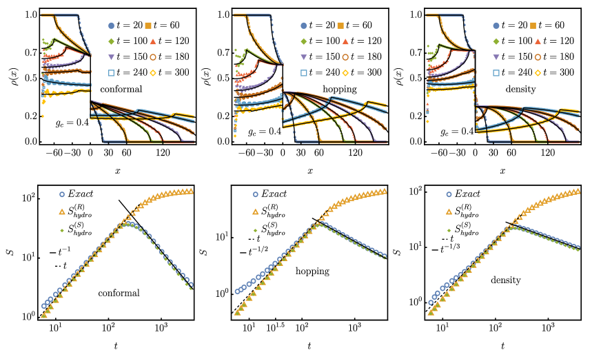
Comparison between exact numerics and hydrodynamics— For the exact numerics, the average current , density or , number fluctuations and the entanglement entropy can be calculated using Eqs. [(8),(9),(12),(10)], while from hydrodynamics, we can calculate these quantities using Eqs. [(14),(15),(16),(Generalised Hydrodynamics description of the Page curve-like dynamics of a freely expanding fermionic gas),(Generalised Hydrodynamics description of the Page curve-like dynamics of a freely expanding fermionic gas)]. In Fig. (2), the top panel shows the density profiles at different times for all three types of defects. We see excellent agreement between exact numerics and hydrodynamics at all times, though we note that hydrodynamics fails to capture the oscillations seen in the density profile from exact numerics. The profiles at early times are the same as obtained in earlier studies for infinite line domain wall evolution Ljubotina et al. (2019); Capizzi et al. (2023). After , which is the time for the fastest particle with speed to make a round trip across the system, the effect of the finite system size shows up in the entire density profile. In the lower panel in Fig. (2), we have plotted the microscopic entanglement entropy from exact numerics and the coarse-grained hydrodynamic entropies computed for system, i.e , and for the reservoir, i.e . We see that at times all three entropies agree and we see a linear growth with time. Beyond this time, the entanglement entropy shows a decay, as expected from the Page curve — we thus refer to as the Page time. Remarkably, beyond the Page time, the entanglement entropy is perfectly reproduced by the system hydrodynamic entropy , both of which show a decay. On the other hand the reservoir hydrodynamic entropy, , shows a monotonic growth beyond the Page time. The long time decay of for all three different defects has the form , expected from hydrodynamics, see Eq. (23). Finite size effects can also be understood completely from the hydrodynamic theory and we show some numerical verifications in Appendix B. In particular we find the scaling form where is a scaling function.
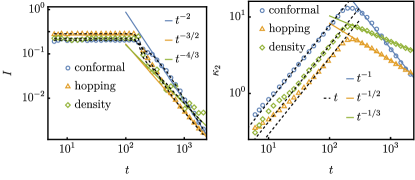
In Fig. (3) we show plots of the dynamics of average current, , and the number fluctuations , again for the three different defect types. Up to , the current is almost constant for all the three defects and the value of the constant current is governed by the transmission probabilities. At long times we again see the decay expected from hydrodynamics (Eq. (23)). Overall, the current behavior is consistent with the form at all times. The number fluctuations closely follows the form of and shows the Page curve like form with identical short and long time scalings. It is worth noting that is a more experimentally accessible quantity than entanglement entropy as mentioned in Klich and Levitov (2009) and thus finding the identical Page curve like dynamics for is interesting and of relevance.
Summary and outlook — To summarize, we considered a freely expanding fermionic gas for which the detailed dynamical structure of the Page curve for entanglement was elucidiated through exact numerics and analytic calculations based on semiclassical generalized hydrodynamics. We investigated spatial density profiles, current and entanglement entropy and show that generalized hydrodynamics (semiclassical) provides a remarkably accurate description of the microscopic quantum dynamics. In this setup, a defect at the system-reservoir interface is crucial for generating entanglement and we studied different defect types. We showed that the early time growth of entanglement is linear, independent of the defect type, while the long time decay depends on the nature of the defect. Interestingly, we observe that the system hydrodynamic entropy captures the full microscopic Page curve while the reservoir hydrodynamic entropy agrees with the Page curve only before the Page time. Beyond this time it appears to grow monotonically. Our approach could be of relevance for further studies on Hawking’s semiclassical calculation and the black hole information paradox.
It will be interesting to study dynamics with other initial conditions such as partial filling fraction, finite temperatures, and to explore the applicability of generalized hydrodynamics (or lack thereof) in such cases. Even in the absence of defects, entanglement entropy for the similar set up shows a logarithmic increase with time and then a decay for a finite system. The logarithmic increase cannot be captured by generalized hydrodynamics and requires one to consider quantum fluctuations Scopa et al. (2021). Understanding the full growth and subsequent decay of entanglement entropy for the defect-free case using quantum fluctuating hydrodynamics will be interesting.
Exploring Page curve-like dynamics for interacting cases, possibly toy models of black holes, and their hydrodynamic description are other fascinating questions.
Acknowledgements — AD thanks Raghu Mahajan for very useful discussions. MS would like to thank Archak Purkayastha for useful discussions. MK and AD acknowledge support from the Department of Atomic Energy, Government of India, under Project No. RTI4001. MK and AD thank the VAJRA faculty scheme (No. VJR/2019/000079) from the Science and Engineering Research Board (SERB), Department of Science and Technology, Government of India. AD acknowledges the J.C. Bose Fellowship (JCB/2022/000014) of the Science and Engineering Research Board of the Department of Science and Technology, Government of India.
Appendix A Analytical long time and short time behavior of current, hydrodynamic entropy for different defects
Using phase space density from hydrodynamic description, it is possible to calculate density , average current and hydrodynamic entanglement entropy or . The formula for phase space density for is given as,
| (25) | ||||
For we get,
| (26) |
where,
| (27) |
For conformal defect, where and are independent of , density can be calculated analytically using Eq. (14) for all time as,
| (28) | |||
where the symbol in the summation index stands for Floor function, i.e., largest integer less than or equal to . Next we discuss details of density, current and hydrodynamic entropy for all defects before the Page time .
A.1 Density, current, entropy before the Page time ()
In this subsection, we will discuss the case where the time is below the Page time.
Phase space density: To see the behavior before the Page time, we can set and in the phase space density given in Eq. (25) and Eq. (A). For , the phase space density can be written as,
| (29) |
while for , it is
| (30) |
with
| (31) | ||||
Density: Using Eq. (29) and Eq. (30), we can write the formula for density for both and as,
| (32) | ||||
Conformal defect: For conformal defect, and using Eq. (32), we find
| (33) | ||||
Hopping defect: For hopping defect [Eq. 4], we get,
| (34) |
Note that putting , in Eq. (A.1), gives us the density profile in the defectless case.
Density defect: In the case of density defect, the transmission probability [see Eq. (4)] is not symmetric about . The maximum value of corresponds to the which is not . The expressions for and are given by,
| (35) | ||||
Again, the special case in Eq. (35), gives the densities in absence of any defect.
Current: Using the expression for density in Eq. (32) and its continuity equation , the current is given by . For our set-up, before the Page time, the formula for current can be written as,
| (36) |
We now give the analytical expressions for various kinds of defect.
Conformal defect: Using Eq. (36), we get .
Hopping defect: For hopping defect, the analytical form of current is
| (37) |
Density defect: For density defect, the analytical form of current is,
| (38) | ||||
Hydrodynamic entropy: Before the Page time, calculating hydrodynamic Yang-Yang entropy from both the system’s phase space density and reservoir’s phase space density give identical result. Thus, here we calculate . Using Eq. (32), we can write the formula for as,
| (39) |
Eq. (A.1) further simplifies to
| (40) | |||
Therefore, for any defect the early time entropy is always linear in . The coefficient of the linear term [see Eq. (40)] depends on the nature of the defect. In the case of conformal defect, Eq. (40) can be calculated exactly and the analytical form is given by,
| (41) |
In principle, before the Page time, one can calculate the analytical expressions for other defects also. We have presented only the conformal defect here for the sake of brevity.
A.2 Density, current, entropy after the Page time ()
In this subsection, we will discuss the case where the time is larger than the Page time.
Following the Poisson summation, we can write the below formula,
| (42) |
Using Eq. (25) and applying the above formula , we get
| (43) | ||||
After performing the integration over and then extracting the long-time limit by putting in Eq. (43), we get,
| (44) |
Similarly for , using Eq. (26), we can write the long-time phase space density as,
| (45) |
Using both Eq. A.2 and Eq. 45, we get an identical expression for absolute value of current ,
| (46) |
We now present further analytical results for the case of conformal defect.
Conformal defect: For conformal defect, it turns out that the density profile can be computed using Eq. (A.2) and Eq. (45) as,
| (47) |
| (48) |
where and are Struve and modified Bessel function of the first kind respectively Olver (2010), and the coefficient is given by
| (49) |
Using the large argument expansion of Struve and Bessel function, the density profiles for both and can be further simplified to,
| (50) |
Therefore, for both and , the density at any given point in space decays as .
Using the expression of current in Eq. (46), for conformal defect, we get the analytical expression,
| (51) |
Our result in Eq. (51) exactly matches with the current that we get from exact numerics and generalized hydrodynamics with no long time approximation [see Fig. 3]. For non-conformal defects, the explicit expressions of current is somewhat cumbersome. However, the very long time limit turns out to be , quite different from the behaviour for conformal defects seen in Eq. (51). This can be argued by taking small limit in the integrand of Eq. (46). For both types of non-conformal defects, at very long times, Eq. (46) takes the form
| (52) |
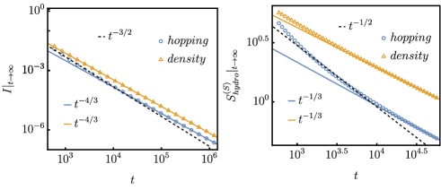
where and are independent of and depend of details of the non-conformal defects. We have shown in Fig. (A1) that for non-conformal defects such as hopping and density defects, current eventually shows scaling consistent with Eq. (52).
We now calculate the Yang-Yang hydrodynamic entropy using Eq. (A.2) and Eq. (45). We first consider the case when the hydrodynamic entropy is calculated from the system. For , the following approximation holds,
| (53) |
We then evaluate Eq. (15) to get . Then using, large-argument expansions of Struve and Bessel functions, we can simplify Eq. (16) to get as
| (54) |
With,
| (55) |
Above Eq. (54), clearly explains the long-time Page curve decay in presence of conformal defect. Therefore, the hydrodynamic entropy calculated from the system gives the correct entanglement entropy. For the other non-conformal defects (density and hopping), shows scaling in the long-time limit which we have shown in Fig. (A1). The analytical reasoning for this is similar to the one discussed for the case of current [see Eq. (52)].
Appendix B Finite size effects: behaviors of density, current, entanglement entropy for other system sizes
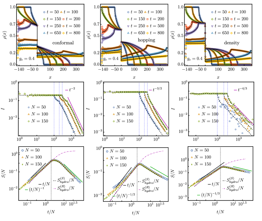
Here we briefly discuss finite size effects and present results for other system sizes. We have shown in Fig. (A2) that all the analysis of density, current, entanglement entropy and hydrodynamic entropy hold for other system sizes and all the features remain the same. The only fact is that finite system size appears in Page time and thus enters into the physical quantities after the Page time .
References
- Eisert et al. (2010) J. Eisert, M. Cramer, and M. B. Plenio, Reviews of modern physics 82, 277 (2010).
- Nishioka (2018) T. Nishioka, Reviews of Modern Physics 90, 035007 (2018).
- Latorre and Riera (2009) J. I. Latorre and A. Riera, Journal of Physics A: Mathematical and Theoretical 42, 504002 (2009).
- Calabrese and Cardy (2009) P. Calabrese and J. Cardy, Journal of Physics A: Mathematical and Theoretical 42, 504005 (2009).
- Coppola et al. (2022) M. Coppola, E. Tirrito, D. Karevski, and M. Collura, Phys. Rev. B 105, 094303 (2022).
- Liu and Vardhan (2021) H. Liu and S. Vardhan, Journal of High Energy Physics 2021, 88 (2021).
- Calabrese and Cardy (2005) P. Calabrese and J. Cardy, Journal of Statistical Mechanics: Theory and Experiment 2005, P04010 (2005).
- Calabrese and Cardy (2007) P. Calabrese and J. Cardy, Journal of Statistical Mechanics: Theory and Experiment 2007, P10004 (2007).
- Alba et al. (2021) V. Alba, B. Bertini, M. Fagotti, L. Piroli, and P. Ruggiero, Journal of Statistical Mechanics: Theory and Experiment 2021, 114004 (2021).
- Alba and Calabrese (2017a) V. Alba and P. Calabrese, Proceedings of the National Academy of Sciences 114, 7947 (2017a).
- Eisler and Bauernfeind (2017) V. Eisler and D. Bauernfeind, Phys. Rev. B 96, 174301 (2017).
- Žnidarič (2020) M. Žnidarič, Communications Physics 3, 100 (2020).
- Bertini et al. (2018) B. Bertini, M. Fagotti, L. Piroli, and P. Calabrese, Journal of Physics A: Mathematical and Theoretical 51, 39LT01 (2018).
- Dubail et al. (2017) J. Dubail, J.-M. Stéphan, J. Viti, and P. Calabrese, SciPost Phys. 2, 002 (2017).
- Fagotti and Calabrese (2010) M. Fagotti and P. Calabrese, Journal of Statistical Mechanics: Theory and Experiment 2010, P04016 (2010).
- Scopa et al. (2021) S. Scopa, A. Krajenbrink, P. Calabrese, and J. Dubail, Journal of Physics A: Mathematical and Theoretical 54, 404002 (2021).
- Eisler and Peschel (2010) V. Eisler and I. Peschel, Annalen der Physik 522, 679 (2010).
- Gamayun et al. (2020) O. Gamayun, O. Lychkovskiy, and J.-S. Caux, SciPost Phys. 8, 036 (2020).
- Song et al. (2011) H. F. Song, C. Flindt, S. Rachel, I. Klich, and K. Le Hur, Phys. Rev. B 83, 161408 (2011).
- Ares et al. (2022) F. Ares, S. Scopa, and S. Wald, Journal of Physics A: Mathematical and Theoretical 55, 375301 (2022).
- Eisler and Peschel (2012) V. Eisler and I. Peschel, Europhysics Letters 99, 20001 (2012).
- Capizzi et al. (2023) L. Capizzi, S. Scopa, F. Rottoli, and P. Calabrese, Europhysics Letters 141, 31002 (2023).
- Ho and Abanin (2017) W. W. Ho and D. A. Abanin, Physical Review B 95, 094302 (2017).
- Kim and Huse (2013) H. Kim and D. A. Huse, Physical review letters 111, 127205 (2013).
- Page (1993) D. N. Page, Physical review letters 71, 3743 (1993).
- Page (2013) D. N. Page, Journal of Cosmology and Astroparticle Physics 2013, 028 (2013).
- Hawking (1975) S. W. Hawking, Communications in mathematical physics 43, 199 (1975).
- Almheiri et al. (2021) A. Almheiri, T. Hartman, J. Maldacena, E. Shaghoulian, and A. Tajdini, Reviews of Modern Physics 93, 035002 (2021).
- Raju (2022) S. Raju, Physics Reports 943, 1 (2022).
- Mathur (2009) S. D. Mathur, Classical and Quantum Gravity 26, 224001 (2009).
- Maes (2015) C. Maes, The European Physical Journal Plus 130, 1 (2015).
- Kehrein (2023) S. Kehrein, arXiv:2311.18045 (2023).
- Glatthard (2024) J. Glatthard, arXiv:2401.06042 (2024).
- Yu et al. (2023) X.-H. Yu, Z. Gong, and J. I. Cirac, Physical Review Research 5, 013044 (2023).
- Bianchi et al. (2022) E. Bianchi, L. Hackl, M. Kieburg, M. Rigol, and L. Vidmar, PRX Quantum 3, 030201 (2022).
- Bianchi et al. (2021) E. Bianchi, L. Hackl, and M. Kieburg, Physical Review B 103, L241118 (2021).
- Bhattacharjee et al. (2021) B. Bhattacharjee, P. Nandy, and T. Pathak, Physical Review B 104, 214306 (2021).
- Pandey et al. (2023) S. Pandey, J. M. Bhat, A. Dhar, S. Goldstein, D. A. Huse, M. Kulkarni, A. Kundu, and J. L. Lebowitz, Journal of Statistical Physics 190, 142 (2023).
- Ljubotina et al. (2019) M. Ljubotina, S. Sotiriadis, and T. Prosen, SciPost Phys. 6, 004 (2019).
- Peschel and Eisler (2009) I. Peschel and V. Eisler, Journal of physics a: mathematical and theoretical 42, 504003 (2009).
- Klich and Levitov (2009) I. Klich and L. Levitov, Phys. Rev. Lett. 102, 100502 (2009).
- Eisler and Rácz (2013) V. Eisler and Z. Rácz, Phys. Rev. Lett. 110, 060602 (2013).
- Castro-Alvaredo et al. (2016) O. A. Castro-Alvaredo, B. Doyon, and T. Yoshimura, Physical Review X 6, 041065 (2016).
- Bertini et al. (2016) B. Bertini, M. Collura, J. De Nardis, and M. Fagotti, Physical review letters 117, 207201 (2016).
- Doyon (2020) B. Doyon, SciPost Physics Lecture Notes , 018 (2020).
- Essler (2022) F. H. Essler, Physica A: Statistical Mechanics and its Applications , 127572 (2022).
- Alba and Calabrese (2017b) V. Alba and P. Calabrese, Phys. Rev. B 96, 115421 (2017b).
- Bertini et al. (2022) B. Bertini, K. Klobas, V. Alba, G. Lagnese, and P. Calabrese, Phys. Rev. X 12, 031016 (2022).
- Olver (2010) F. W. Olver, NIST handbook of mathematical functions hardback and CD-ROM (Cambridge university press, 2010).