CafkNet: GNN-Empowered Forward Kinematic Modeling for Cable-Driven Parallel Robots

Abstract

When deploying Cable-Driven Parallel Robots (CDPRs) in practice, one of the challenges is kinematic modeling. Unlike serial mechanisms, CDPRs have a simple inverse kinematics problem but a complex forward kinematics (FK) issue. Therefore, the development of accurate and efficient FK solvers has been a prominent research focus in CDPR applications. By observing the topology within CDPRs, in this letter, we propose a graph-based representation to model CDPRs and introduce CafkNet, a fast and general FK solver, leveraging Graph Neural Network (GNN). Extensive experiments are conducted on 3D and 2D CDPRs across various configurations, including under-constrained, fully-constrained, and over-constrained cases, in both simulation environments and real-world scenarios. The experimental results showcase that CafkNet can learn the internal topological information of CDPRs and accurately solve the FK problem as an FK solver. Furthermore, training the CafkNet model on partial configurations enables zero-shot generalization to other configurations. Lastly, CafkNet effectively bridges the sim2real gap by using both simulation data and part of real-world data. To the best of our knowledge, it is the first study that employs the GNN to solve FK problem for CDPRs.

I Introduction

Cable-driven parallel robots (CDPRs) are a kind of parallel mechanism that employs flexible cables to replace rigid links [1, 2, 3, 4]. It has exhibited excellent scalability in terms of size, payload, and dynamics capacities.

The most crucial step before deploying CDPRs is modeling, including kinematic modeling (KM) and dynamics modeling (DM). KM refers to the process of creating a mathematical equation of the end-effector movement, including its kinematic parameters such as position, orientation, and velocity. DM, on the other hand, is the process of creating a mathematical representation of how the end-effector will respond to external forces over time. For the KM of CDPR, the usual practice, like [5], is to first determine the configuration of the CDPR according to the application requirements, including the number of cables, positions of the pulley on the framework, the shape of the end-effector and the position on which the cable is connected. Then, according to the geometric relationship, the modeling of cable attachment on the end-effector and anchor points on the framework is formulated. After that, some downstream tasks can be completed, such as workspace determination [6], path planning [7], and control [8]. In CDPR’s KM, there are typically two types of calculations: forward kinematics (FK) and inverse kinematics (IK). FK involves determining the end-effector pose (i.e., position and orientation) based on cable lengths, while IK solves for the length of cables given the end-effector pose in reverse. In contrast to the traditional serial mechanical structure, the FK problem of CDPRs is more complex than its IK.

Therefore, numerous works focus on solving FK problems of CDPRs. [9] discusses the non-trivial computation of the FK of cable-driven parallel robots, which are kinematically over-constrained mechanisms. In addition, [1] provides the overview of FK solvers based on successful application cases of CDPRs. Recent work [10] proposes a neural network approach for solving the FK of under-constrained cable-driven parallel robots. In summary, solving the FK for CDPRs presents several challenges.

1. Nonlinearity. Solving the FK problem for CDPRs, especially when over-constrained, is challenging due to its non-linear nature in FK formulations.

2. Flexibility of Configuration. CDPRs offer customizable cable configurations, but modeling each configuration separately creates additional work.

3. Sim2Real Gap. The gap between the simulated and real-world performance of CDPRs is inevitable due to limited model accuracy and complex cable systems.

It is obvious that due to the nonlinearity and complexity of FK problems, FK solvers have a large computational burden and also suffer from the problem of no solution or multiple solutions. Furthermore, configuration-dependent FK solvers cannot be easily applied to the reconfiguration CDPR (RCDPR) [11] or the case of simply adding or subtracting some cables. However, according to observations in [12], we notice that the change of CDPR’s configuration does not affect the topological architecture if its configuration can be represented as a graph. In addition, it is an indisputable fact that the Sim2Real gap is inevitable, despite significant efforts to reduce differences [13, 14, 15]. This is due to the difficulty of measuring and modeling systematic errors (cable attachment position errors) and random errors (cable sagging) in CDPR, some of which are even unknowable. One promising approach currently being explored is using real data to learn about these errors, as it has been shown to be an effective way to bridge the gap.

In this paper, we propose an FK solver based on Graph Neural Networks (GNN) for CDPR, denoted by CafkNet. By utilizing the proposed graph representation of CDPR, the CafkNet can rapidly learn the underlying topological structure of CDPR and serve as an FK solver to solve FK problems. Thanks to the topological similarity of graphs, CafkNet trained from a specific configuration can be easily transferred to other configurations without fine-tuning. Additionally, CafkNet performs well in bridging the Sim2Real gap between vast easily accessible simulation data and limited expensive real-world data. We have conducted extensive simulations and real-world experiments to demonstrate the modeling capabilities of CafkNet. To the best of our knowledge, it is the first study to employ the GNN for FK problem of CDPRs.

Main contributions:

• We propose a forward kinematic modeling method based on GNN, CafkNet, which is the first GNN-empowered FK solver for CDPRs.

• We use graph similarity to enable zero-shot and few-shot transfer learning, allowing CafkNet to quickly transfer its knowledge from one configuration to others.

• We employ CafkNet to bridge the Sim2Real gap in CDPR, which has been verified in simulation and real machine experiments.

The rest of the paper is organized as follows. Sec. II reviews related studies about KM of CDPR and GNN applications in robotics. Sec. III details the CDPR geometric model. Sec. IV introduces the proposed graph representation of CDPR and the architecture of CafkNet. Then, Sec. V demonstrates the experiment details followed by modeling results of CafkNet in Sec. VI. Finally, the conclusion and outlook are presented in Sec. VII.

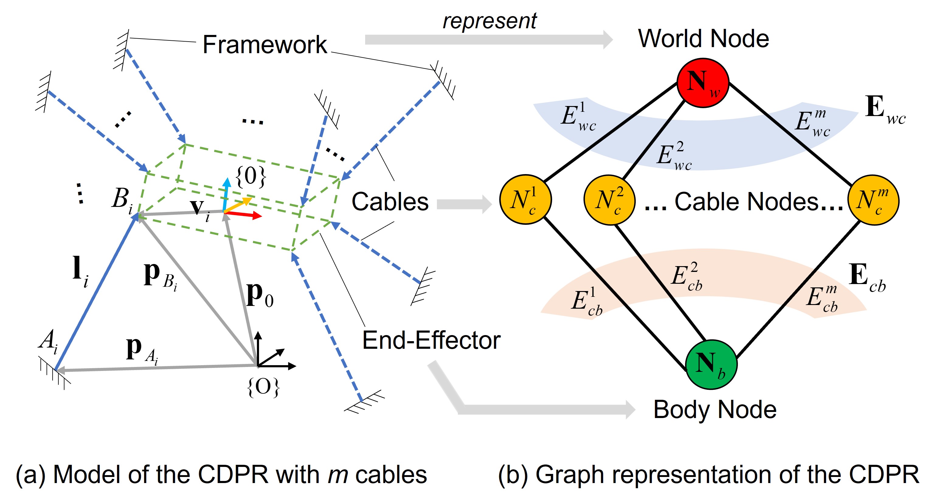
Figure 1: Workflow of CafkNet. (a) The geometric model of a CDPR with $m$ cables. (b) The proposed graph presentation for the CDPR.

II Related work

II-A Kinematic Modeling of CDPR

KM is a fundamental problem in CDPR’s studies and also the first step in each CDPR’s application, as revealed in [1, 2, 3]. In CDPR, the IK problem, i.e., the rope length determination given the end-effector pose, is easy to solve, relative to the FK issue. Due to the nonlinearities in FK, there are three potential situations when solving FK [16], i.e., no solution, one solution, and multiple solutions. In addition, [9] introduces an FK solver based on energy minimization for a numerical optimization technique. Also, [17] takes into account the nonlinearities of cables and proposes a method for solving the FK of CDPRs with sagging cables. However, these methods are mainly used to model CDPR more finely under their respective configurations, so as to complete the optimization of FK. More generally, some studies [18, 17] provide the FK solver using graph and graph theory to model the CDPR. Recent works employ diverse machine learning methods trying to solve the system modeling problem, such as neural networks [19, 10], deep learning [20], etc. Although their results validate the feasibility of neural networks on FK, they still need to be retrained when changing their configurations. In this work, we combine the graph and neural network and utilize GNN to represent and model the CDPR kinematics. Benefitting from GNN, the proposed CafkNet method could transfer its learned topological structure of CDPR to other configurations without retraining.

II-B Graph Neural Networks in Robotics

Recently, data-driven methods have emerged as an effective approach to approximate robotics modeling. Given the fact that the robot’s structure can be easily represented as a graph, where joints are denoted as nodes and links are denoted as edges, GNNs have been increasingly applied in robotics sensing [21, 22], modeling [23, 24, 25], and control [26, 27, 28, 29].  [21, 22] propose to use GNN to encode the distributed tactile sensing information for downstream tasks. [23, 24] propose using GNN to model system dynamics, where graphs represent the rigid bodies.  [25] aims to find the representation of robot data, including kinematic data and motion data using the GNN message computation scheme. NerveNet [26] seeks to train a generalized control policy that can transferred to other robot configurations.  [27, 28, 29] propose a similar idea to train a structure-agnostic locomotion policy with a novel message-passing scheme. This paper is the first work to employ the GNN technique to solve the FK issues for the CDPRs.

III Background

III-A Geometric Model of CDPR

A 6-degree-of-freedom (DoF) spatial CDPR is illustrated in Fig. 1-(a), where two endpoints of the $i$-th cable ($i=1,2,\cdots,m$) are denoted by $A_{i}$ and $B_{i}$. Given the geometric relationship, the cable vector $\mathbf{l}_{i}$ can be determined as follows.

$$\mathbf{l}_{i}=\mathbf{p}_{B_{i}}-\mathbf{p}_{A_{i}},$$ (1)

where $\mathbf{p}_{B_{i}}=\mathbf{p}_{0}+R~{}\mathbf{v}_{i}$. Here $\mathbf{p}_{0}=[x,y,z]^{T}$ refers to the position of end-effector in the world frame $\{O\}$ (i.e., framework), and $R$ is the rotation matrix from the body frame $\{0\}$ attached on the end-effector to the world frame $\{O\}$. Additionally, $\mathbf{v}_{i}$ is a position vector of the vertice $V_{i}$ expressed in $\{0\}$, which is constant and determined by the cable attachment position on the end-effector. So it is clear that $\mathbf{p}_{A_{i}}$ and $\mathbf{p}_{B_{i}}$ are position vectors of $A_{i}$ and $B_{i}$ represented in $\{O\}$, respectively.

III-B Kinematics of CDPR

Here we can define the pose of end-effector in the task space of CDPR as $\mathbf{Q}=[x,y,z,\phi,\theta,\psi]^{T}$, where $\phi,\theta,\psi\in[-\pi,\pi]$ are Euler angles of end-effector for roll, pitch, yaw, respectively and they are involved in rotation matrix $R$ in (1). In addition, its joint space can be defined by a set of cable vectors $\mathbf{L}=\{\mathbf{l}_{1},\cdots,\mathbf{l}_{m}\}$, accordingly. Thus, the IK and FK problems can be formulated as

IK: $$\mathbf{L}=f_{IK}(\mathbf{Q}),$$ (2)

FK: $$\mathbf{Q}=f_{FK}(\mathbf{L}).$$ (3)

It is straightforward to find the (1) is equivalent to the function $f_{IK}$ in (2), i.e., solving cable length $\mathbf{l}_{i}\in\mathbf{L}$ (joint space) from end-effector pose $\mathbf{Q}$ (task space). For FK problem, however, things are no longer so simple. In general, the FK is formulated as an optimization problem, that minimizes the error between the given cable lengths ${\mathbf{L}}$ and lengths determined from IK at one pose $\mathbf{Q}$, that is,

$$\begin{split}\mathop{\arg\min}_{\mathbf{Q}}&\ \|{\mathbf{L}}-f_{IK}(\mathbf{Q}))\|^{2},\\ \textrm{s.t.}\quad&\mathbf{Q}_{lb}\leq\mathbf{Q}\leq\mathbf{Q}_{ub}.\end{split}$$ (4)

Here $\mathbf{Q}_{lb}$ and $\mathbf{Q}_{ub}$ refer to the lower bounds and upper bounds prescribed to the pose $\mathbf{Q}$.

IV Methodology

IV-A Graph Representation of CDPRs

A graph typically consists of nodes and edges. In this work, we define three types of nodes and two types of edges to represent the CDPR to a graph, as outlined in Fig. 1-(b). Based on the geometric structure of CDPR in Fig. 1-(a), the framework can be considered as a world node $\mathbf{N}_{w}$, and the end-effector is seen as a body node $\mathbf{N}_{b}$. Furthermore, the position of the world frame $\{O\}$ attached to the framework, i.e., $[0,0,0]$, is set as the initial feature of $\mathbf{N}_{w}$. Similarly, the pose $\mathbf{Q}$ of the body frame attached to the end-effector is selected as the node feature of $\mathbf{N}_{b}$. For forward kinematic modeling, $\mathbf{Q}$ is unknown at first, so its node feature is initialized to be $[0,0,0,0,0,0]$. For CDPRs, cables connecting the framework and the end-effector are defined as a set of cable nodes $\mathbf{N}_{c}=\{N_{c}^{1},N_{c}^{2},\cdots,N_{c}^{m}\}$ for $m$ cables. Here $N_{c}^{i}$ refers to the $i$-th cable node, and its initial feature is the cable length, i.e., the scalar $||\mathbf{l}_{i}||$ in (1). In addition, the connection of the cable to framework and the connection to end-effector are considered as two types of edges, $\mathbf{E}_{wc}$ and $\mathbf{E}_{cb}$, whose edge features $e^{i}_{wc}$ and $e^{i}_{cb}$ for $i$-th cable are the attachment position vectors $A_{i}$ and $B_{i}$ in (1), respectively. As such, the CDPR can be formulated as a graph $G$ as

$$G=(\mathbf{N}_{w},\mathbf{N}_{c},\mathbf{N}_{b},\mathbf{E}_{wc},\mathbf{E}_{cb}).$$ (5)

Algorithm 1 GNN-Empowered Forward Kinematic

1:Input: Graph representation of CDPR $G$ in (5)

2:Output: Pose prediction of the end-effector $\mathbf{Q}$

3:Encoder:

4:for each node and edge $u$ in the graph $G$ do

5:     Initialize node feature $h_{u}$ by (6)

6:end for

7:Message Propagation:

8:for $s=1$ to $N$ do $\triangleright$ $N$ stacked message propagation blocks

9:     for each cable node $i$ do

10:         Compute message $m_{w,c}^{i}$ by $\gamma_{wc}$ in (7)

11:         Update cable node feature $h_{c}^{i}$ by (8)

12:     end for

13:     Initialize an empty set $\{\}$ for body node messages

14:     for each cable node $i$ do

15:         Compute message $m_{c,b}^{i}$ by $\gamma_{cb}$ in (9)

16:         Add $m_{c,b}^{i}$ to the set $\{m^{i}_{c,b}\}$

17:     end for

18:     Update body node feature $h_{b}$ by (10)

19:end for

20:Decoder:

21:Decode the final body node feature to pose prediction of the end-effector by (11).

IV-B GNN-Empowered Forward Kinematic Modeling

In this subsection, we will parameterize the FK problem of CDPRs as a GNN using the Encoder-Propagation-Decoder format [30] for message passing, as summarised in Algo. 1.

Encoder: The encoder receives a graph $G$ in (5) representing a CDPR, then it maps each node feature and edge feature to a fixed-dimension embedding by

$$h_{u}=\sigma_{in}(x_{u}),~{}u\in\{w,c,b,wc,cb\},$$ (6)

where $\sigma_{in}$ denotes the initialization multi-layer perceptron (MLP). Here $x_{u}$ and $h_{u}$ refer to the initial and hidden features of node (or edge) $u$, respectively.

Message Propagation: The propagation model consists of $N$ stacked message propagation blocks to update node embedding, which means message computation and aggregation are recurrently applied $N$ times. In each message propagation block, a top-down message-passing scheme is adopted. Specifically, the model first computes the message from the world node to each cable node $i$ by

$$m^{i}_{w,c}=\gamma_{wc}(h_{w},h^{i}_{c},e^{i}_{wc}),$$ (7)

where $\gamma_{wc}$ refers to the MLP from world to cable nodes. Then, $h_{w}$ and $h^{i}_{c}$ are hidden features of the world node and the $i$-th cable node, respectively, then $e^{i}_{wc}$ is the edge feature of the edge between the world node and the $i$-th cable node. Once every node finishes computing messages, the hidden feature of every cable node $h^{i}_{c}$ can be updated based on the message computation and itself:

$$h^{i}_{c}=\max(\{h^{i}_{c},m^{i}_{w,c}\}),$$ (8)

Similarly, the message from the $i$-th cable node to the body node is computed by

$$m^{i}_{c,b}=\gamma_{cb}(h^{i}_{c},h_{b},e^{i}_{cb}),$$ (9)

where $\gamma_{cb}$ denotes the MLP from cable to body nodes. After messages of all cable nodes $\{m^{i}_{c,b}\}$ are calculated, the body node is updated via

$$h_{b}=\max(\{h_{b},\{m^{i}_{c,b}\}\}).$$ (10)

Note that, as shown from line 9 to line 18 in Algo. 1, we only employ two message computation functions, i.e., $\gamma_{wc}$ and $\gamma_{cb}$, to handle the message propagation on two types of edges in the proposed graph representation. Thus, the same type of edges share MLP parameters.

Decoder: In the decoder, the output MLP $\sigma_{out}$ takes the final hidden feature of body node $h_{b}$ after $N$ propagation blocks as input and outputs the pose of end-effector $\mathbf{Q}$, as formulated by

$$\mathbf{Q}=\sigma_{out}(h_{b}).$$ (11)

IV-C Transfer Learning across Configurations

CafkNet employs parameter sharing among identical node relationships, enhancing its ability to perform structural transfer tasks effectively. Specifically, there are only two parameterized MLPs in our graph for message propagation, including $\gamma_{wc}$ for the relationship between world node and cable node, as well as $\gamma_{cb}$ for the relationship between cable node and body node. The parameters of MLPs are independent of cable number. As a result, our approach facilitates the application of the kinematic model to various CDPR configurations, significantly improving generalization capabilities across different cable arrangements. Extensive experiments in Sec. VI verify the transferability of our CafkNet.

V Experiments

V-A Dataset

In this work, we take $8$ configurations of CDPR into consideration, including spatial ones (e.g., Fig. 2-(a) and (b)) and planar ones (e.g., Fig. 2-(c) and (d)). We investigate under-constrained, fully-constrained and over-constrained cases, ranging from four cables to ten cables. The cable attachment locations in each configuration are detailed in Tab. I, where $A_{i}$ refers to $\mathbf{p}_{A_{i}}$ in (1), and $B_{i}$ indicates $\mathbf{v}_{i}$ in (1). In addition, we validate our method in the real experiment setup, as shown in Fig. 2-(c)

In the simulator, we randomly generate $100$ polynomial trajectories for each configuration, as shown in dashed curves in Fig. 2 and then uniformly sample $100$ poses along each trajectory. Furthermore, the cable lengths at each pose can be simply calculated via IK at each configuration. In the real experimental setup, the pose of the end-effector could be determined by the external motion capture system, OptiTrack (NaturalPoint Inc., USA), using attached markers in the end-effector and anchors, as depicted in Fig. 2-(c). The cable lengths are measured by the motor encoders accordingly. We partition the dataset into a training set comprising $80\%$ of the data and a testing set containing the remaining samples.

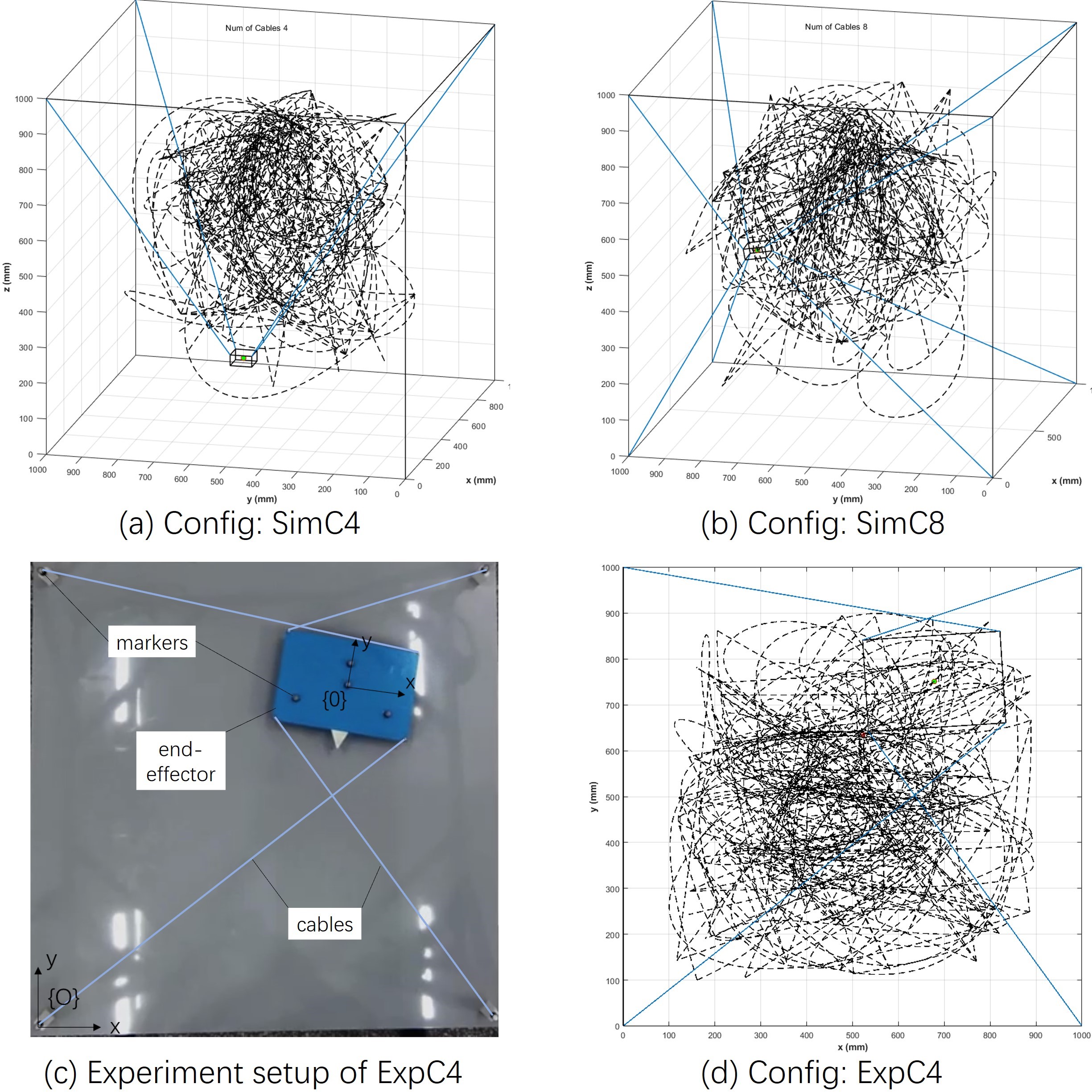
Figure 2: Configurations of CDPR in simulation and experiment scenarios. In simulation cases, we randomly generate $100$ polynomial trajectories (dashed curves) and sample $100$ poses (including position and orientation) along each trajectory.

TABLE I: Cable Attachment Locations for Various Configurations

Config.	SimC4	SimC5	SimC6		SimC7		SimC8		SimC9		SimC10		ExpC4
$A_{i}$	(0.0, 1.0, 1.0)	(0.5, 0.5, 1.0)	(0.5, 1.0, 0.0)	(1.0, 1.0, 1.0)	(0.1, 1.0, 0.0)	(1.0, 1.0, 1.0)	(0.0, 1.0, 0.0)	(0.0, 1.0, 1.0)	(0.1, 1.0, 0.0)	(1.0, 0.0, 1.0)	(0.1, 1.0, 0.0)	(1.0, 1.0, 1.0)	(0.0, 0.0, 0.0)
	(1.0, 1.0, 1.0)	(0.0, 1.0, 1.0)	(0.5, 0.0, 0.0)	(1.0, 0.0, 1.0)	(0.9, 1.0, 0.0)	(1.0, 0.0, 1.0)	(1.0, 1.0, 0.0)	(1.0, 1.0, 1.0)	(0.9, 1.0, 0.0)	(0.0, 0.0, 1.0)	(0.9, 1.0, 0.0)	(1.0, 0.0, 1.0)	(1.0, 0.0, 0.0)
(m)	(1.0, 0.0, 1.0)	(1.0, 1.0, 1.0)	(0.0, 1.0, 1.0)	(0.0, 0.0, 1.0)	(0.5, 0.0, 0.0)	(0.0, 0.0, 1.0)	(1.0, 0.0, 0.0)	(1.0, 0.0, 1.0)	(0.5, 0.0, 0.0)	(0.0, 0.5, 0.0)	(0.9, 0.0, 0.0)	(0.0, 0.0, 1.0)	(1.0, 1.0, 0.0)
	(0.0, 0.0, 1.0)	(1.0, 0.0, 1.0)			(0.0, 1.0, 1.0)		(0.0, 0.0, 0.0)	(0.0, 0.0, 1.0)	(0.0, 1.0, 1.0)	(1.0, 0.5, 0.0)	(0.1, 0.0, 0.0)	(0.0, 0.5, 0.0)	(0.0, 1.0, 0.0)
		(0.0, 0.0, 1.0)							(1.0, 1.0, 1.0)		(0.0, 1.0, 1.0)	(1.0, 0.5, 0.0)
$B_{i}$	(-30, 30, 15)	(0, 0, 15)	(0, 30, 15)	(30, 30, -15)	(-25.5, 30, 15)	(30, 30, -15)	(-30, 30, -15)	(-30, 30, 15)	(-25.5, 30, 15)	(30, -30, -15)	(-25.5, 30, 15)	(30, 30, -15)	(150, -100, 0)
	(30, 30, 15)	(-30, 30, 15)	(0, -30, 15)	(30, -30, -15)	(25.5, 30, 15)	(30, -30, -15)	(30, 30, -15)	(30, 30, 15)	(25.5, 30, 15)	(-30, -30, -15)	(25.5, 30, 15)	(30, -30, -15)	(-150, -100, 0)
(mm)	(30, -30, 15)	(30, 30, 15)	(-30, 30, -15)	(-30, -30, -15)	(0, -30, 15)	(-30, -30, -15)	(30, -30, -15)	(30, -30, 15)	(0, -30, 15)	(-30, 0, 15)	(25.5, -30, 15)	(-30, -30, -15)	(-150, 100, 0)
	(-30, -30, 15)	(30, -30, 15)			(-30, 30, -15)		(-30, -30, -15)	(-30, -30, 15)	(-30, 30, -15)	(30, 0, 15)	(-25.5, -30, 15)	(-30, 0, 15)	(150, 100, 0)
		(-30, -30, 15)							(30, 30, -15)		(-30, 30, -15)	(30, 0, 15)

V-B Implementation Details

In this work, we use a supervised learning paradigm to train CafkNet for CDPRs based on the above dataset. Here, the Root Mean Square Error (RMSE) is selected as our performance metric. Note that we only calculate the RMSE loss about positions, disregarding any variations in orientations. In addition, Adam [31] is utilized as the optimizer, with a batch size of $32$. Other parameters, such as the hidden feature dimensions and number of MLP layers in CafkNet, the initial learning rate, and the reduction factor for the learning rate scheduler, are optimized automatically via the toolkit in [32]. All codes are developed using PyTorch and trained on a single NVIDIA GeForce RTX 4090 GPU card.

VI Results and Discussion

VI-A FK Modeling for CDPR

In this subsection, we present the results and time cost of solving the FK problem at numerous CDPR configurations by CafkNet. Additionally, we compare it with the MLP method and the optimization-based FK solver separately.

For CafkNet, we provide two types of FK solutions. The first approach involves training CafkNet using data from a single configuration and solving the FK problem specifically for that configuration. Therefore, each model is dedicated to solving the FK problem for a single configuration, and this approach is referred to as CafkNet (one2one). The second approach involves training a universal CafkNet model using data from all configurations. During the testing phase, the model is divided into multiple heads, each addressing the FK issues for a specific configuration. This method is referred to as CafkNet (multi-task).

As a comparison, we also employ MLP to solve FK problems, where all node features and edge features are as input and output is the position of the end-effector. In addition, an optimization-based FK solver is also used, which takes advantage of the least square method in [33] to solve the optimization problem as formulated in (4), where the $\mathbf{Q}_{lb}$ and $\mathbf{Q}_{ub}$ are set as $[100,100,100,-0.26,-0.26,0]$ and $[900,900,900,0.26,0.26,0]$, respectively. The initial guess is given as $[500,500,500,0,0,0]$.

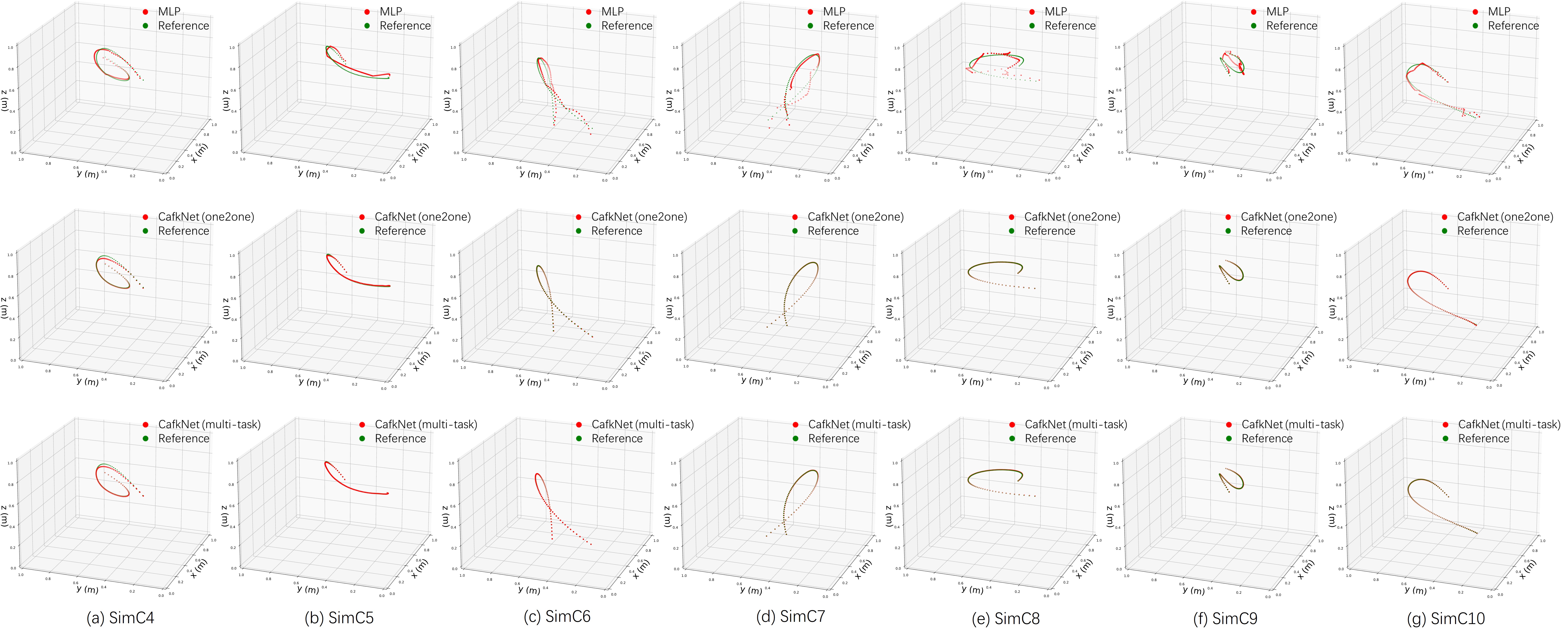
Figure 3: Reference trajectories and resulting trajectories solved by the MLP and CafkNet (including one2one and multi-task cases) at configurations SimC4 to SimC10. Top row: MLP; Middle row: CafkNet (one2one); Bottom row: CafkNet (multi-task).

The results of modeling accuracy, i.e., the RMSE loss of predicted positions and reference positions, as revealed in Tab. II. Here we can observe that the opt. FK solver achieves the smallest error in SimC6 to SimC10 but fails in SimC4 and SimC5, where CafkNet achieves the lowest error. But from SimC6 to SimC10, the errors of CafkNet remain within $1.5$ mm. On the other hand, the MLP solver exhibits the poorest accuracy, with errors exceeding $15$ mm. Furthermore, we notice that the accuracy of CafkNet (multi-task) is comparable to CafkNet (one2one).

However, considering the computational time for FK solving, as shown in Tab. III, the opt. FK solver takes an average time of approximately $1$ s for the best-accuracy configurations, SimC4 $\sim$ SimC10, but experiences a significant time raising at failure cases. In contrast, it can be found that CafkNet (one2one) achieves remarkably low computation time, with only $0.649$ s for SimC4 and a few milliseconds for other configurations. Considering both computational time and solution accuracy, the CafkNet offers a trade-off between low time consumption and relatively high precision, demonstrating significant potential for real-time CDPR applications compared to the opt. FK solver.

Note that the Tab. III indicates the overall time taken by both methods to compute a complete trajectory, comprising 100 FK problems. The resulting trajectories are visually presented in Fig. 3, illustrating the FK outcomes of MLP (top row), CafkNet (one2one) (middle row), and CafkNet (multi-task) (bottom row). The close correspondence observed between the predicted and reference trajectories serves as evidence of the accurate FK solutions.

TABLE II: Modeling Accuracy (unit: mm).
Bold: minimum error in each configuration.

Method		Configuration
		SimC4	SimC5	SimC6	SimC7	SimC8	SimC9	SimC10
Opt. FK Solver		443.00	349.16	0.07	0.00	0.00	0.00	0.00
MLP		18.67	16.45	11.24	17.14	31.51	31.49	15.37
CafkNet	one2one	4.19	2.46	0.42	1.57	1.58	1.61	1.05
	multi-task	4.97	1.27	0.86	1.45	2.39	2.32	0.55

TABLE III: Time Cost of FK solving (unit: s).

Method	Configuration
	SimC4	SimC5	SimC6	SimC7	SimC8	SimC9	SimC10
Opt. FK Solver	51.932	76.245	1.171	1.087	0.993	0.999	1.084
CafkNet (one2one)	0.649	0.002	0.004	0.001	0.001	0.002	0.004

VI-B Transfer Learning in CDPR

In this subsection, we investigate the transferability of our CafkNet, and the resulting modeling errors are given in Tab. IV. In the GNN, all cable and framework node interactions share parameters $\sigma_{C}$, which allows us to transfer the kinematic model to CDPRs with different cable configurations to assess the generalization ability of the trained model. We conduct a series of experiments on transferability tests, where the kinematic model is transferred without further fine-tuning.

We conduct two groups of zero-shot transfer experiments. In the first group (Exp C-1), we train CafkNet on one configuration, e.g., SimC$i$, and then directly apply it to solve the FK problem on other configurations SimC$j$, where $j\neq i$. We calculate the average errors for the resulting positions, i.e., $x,y$, and $z$. In the second group of experiments (Exp C-2), we aim to predict the pose in the configuration SimC$i$ using data from multiple configurations SimC$j$, where $j\in(1,2,..)$ and $j\neq i$ for training. The experiment results are revealed in Tab. IV, where rows 2 to 8 display outcomes of Exp C-1, and row 9 displays the results of Exp C-2.

For example, the second row in Tab. IV represents the training of CafkNet on the data from SimC4, followed by directly solving the FK problems on SimC5-SimC10, respectively. It can be observed that the errors in Exp C-1 are relatively high. This result aligns with our expectations, as CafkNets have limited and singular learning data on a single configuration, resulting in better performance on the same configuration and poorer performance on other configurations.

However, from the results of Exp C-2, i.e., last row in Tab. IV, we discover that due to the increased variety and volume of training data in SimC$j$ for CafkNet, even without prior exposure to configuration SimC$i$, it can still successfully transfer and solve the FK problem in the unseen configuration, showcasing good zero-shot transferability.

It is worth noting that despite the less satisfactory results in Exp C-1, we can also observe that CafkNet, aside from performing well on its own configuration, exhibits increasing accuracy errors as the distance from its own configuration increases. For instance, the model trained on SimC6 demonstrates better accuracy on SimC7 compared to SimC8, and the results on SimC5 are superior to those on SimC4.

TABLE IV: Modeling Accuracy on Transferability of CafkNet (unit: mm). Bold: minimum test error in each configuration.

	SimC4	SimC5	SimC6	SimC7	SimC8	SimC9	SimC10
SimC4	-	14.85	36.11	46.37	41.82	53.24	44.53
SimC5	20.64	-	39.03	49.7	36.23	60.19	50.97
SimC6	64.94	58.45	-	21.07	31.77	25.24	22.72
SimC7	80.06	81.74	14.95	-	43.61	9.29	16.45
SimC8	89.99	88.05	47.17	33.76	-	34.09	21.91
SimC9	20.98	67.05	7.13	9.46	23.38	-	6.04
SimC10	12.29	97.71	5.58	8.12	13.17	7.65	-
multi-config.	4.14	8.23	2.06	1.74	11.96	1.09	0.69

VI-C Bridging Sim2Real Gap

In practical applications of CDPR, noise is inevitable. It can originate from various sources such as the mechanical structure, including the winch and pulley, as well as from the motor encoder and cable extension. Thus the sim2real gap in CDPR should be well studied. To validate the robustness of CafkNet against noisy data, we utilize two datasets in this study. One dataset was generated by injecting Gaussian noise into the data obtained from the simulator. The other dataset was collected from a real experimental platform, as depicted in Fig. 2-(c).

VI-C1 Simulated Data with Artificial Noises

In Fig. 2-(c), we find that the pose of CDPR can be accurately captured by the motion capture system, so we do not add noise to the pose in the simulated data. On the contrary, the main errors in the real experiment come from the length of the cable, including the error of the motor encoder, as well as the position of the cable on the pulley and where it is mounted at the end-effector. Thus, we introduce the random error $\epsilon$ into the simulator mainly from the position noises in attachment positions, i.e., $A_{i}\pm\epsilon,~{}B_{i}\pm\epsilon$, where $\epsilon\sim N(\mu=0,\sigma^{2})$. We conduct two sets of experiments targeting different $\sigma$ values to assess the performance of CafkNet when exposed to artificial noise, i.e., $\sigma=5$ and $\sigma=10$, respectively. In each experimental set, we also consider three categories based on the source of the training and testing data for each CDPR configuration. These categories include:

• Training and testing on simulated data.

• Training on simulated data and testing on noise data.

• Training and testing on noise data.

Here, we define the data collected from the simulator, i.e., from Fig. 2-(d), as simulated data, while the data with artificially added random noise is referred to as noise data.

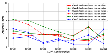
Figure 4: Modeling accuracy of CafkNet working on artificial noise data. Here errors in case 1 to case 3 are generated by $\epsilon\sim N(0,5^{2})$, and errors in case 4 to case 6 are generated by $\epsilon\sim N(0,10^{2})$. $N$ refers to the Gaussian distribution.

The results are demonstrated in Fig. 4. From it, we can observe that as the magnitude of artificially introduced noise increases, the modeling error solved by CafkNet also exhibits a corresponding overall increase. However, the overall increment in modeling error does not exceed a relationship greater than twice the magnitude of the artificial error (i.e., $5$ to $10$), particularly when observing the green curve. In addition, as the number of cables increases, the modeling error from CafkNet gradually decreases and stabilizes below 4mm. We can also find that the resulting curves of case 1 and case 2 are very close, with almost identical computational errors. This indicates that the model trained on clean data demonstrates generalization capability, allowing it to generalize to data with errors even in zero-shot scenarios. A similar phenomenon can be found between case 3 and case 4, as well. As anticipated, if noise data is used during training, CafkNet will provide the lowest error results, as observed in the blue curve.

However, noise data in real-world applications is often obtained from real machine experiments, which can be costly. On the other hand, simulated data is relatively easier to acquire, and its quantity can surpass that of real machine data. Therefore, in the next, we will demonstrate how CafkNet combines low-cost simulated data with a portion of machine data to achieve accurate FK solutions for real-world scenarios.

VI-C2 Real Experimental Data

In this subsubsection, we will present the modeling process for deploying a real CDPR platform, which primarily involves building a model in the simulator based on design blueprints, i.e., Fig. 5-(i), generating simulated trajectories based on tasks in the simulation environment, and conducting simulated operations (Fig. 5-(ii)). Subsequently, the target trajectories are executed on the actual machine (Fig. 5-(iii)). During this process, the CDPR model in the simulation environment can be a replica of the model in the design blueprints, but there will inevitably be parameter discrepancies between the simulated environment and the real platform. Therefore, we demonstrate the sim2real capability of CafkNet.

For this experiment, we primarily have three sources of data, as depicted in Fig. 5. One type of data is defined as simulated data, which consists of randomly sampled trajectories (i.e., pose-length pairs) generated on the simulator, as shown in Fig. 5-(i). Another type of data is defined as clean data, which is generated on the simulation platform specifically for the target trajectory, as illustrated in Fig. 5-(ii). These first two types of data are readily available and do not consider any errors. The last type of data, referred to as noise data, as depicted in Fig. 5-(ii), originates from measurements when the practical CDPR executes the target path. This data includes both systematic errors inherent in the machine (e.g., installation errors in pulleys, shape errors in end-effector) and random errors during execution (e.g., motor encoder errors, measurement errors in the motion compensation system). Systematic errors are unique to each device, and their distribution is specific to the current equipment. In other words, a different set of systematic errors would be observed in another device. Moreover, it is challenging to model random errors.

To evaluate the sim2real capability of CafkNet, we design three methods based on the training data, as presented in Tab. V. Furthermore, in the testing, cable lengths from either the clean data or noise data are inputted into the trained model. Then it solves for the end-effector poses and compares them with the corresponding poses from the clean data and noise data to compute the average error, respectively.

• sim2real: During the training phase, CafkNet is trained using all simulated data and tested all clean data.

• real2real: In the training phase, $80\%$ of the clean data is used, while in the testing phase, the remaining $20\%$ of the clean data or the noise data is used.

• sim&real2real: This method introduces composite training data, which consists of simulated data and $80\%$ of clean data. The testing data remains consistent with the real2real method.

The resulting trajectories solved by CafkNet under these three methods are presented in Fig. 6, and their accuracy results are given in Tab. V. The experimental findings demonstrate that CafkNet, trained using composite data consisting of simulated data and $80\%$ of the clean data, yields end-effector poses that closely align with real machine data. This indicates its effectiveness in bridging the sim2real gap in practical applications of CDPRs. Specifically, when testing on clean data, as expected, the sim2real method exhibits the lowest error, followed by sim&real2real, while real2real performs the poorest. This can be attributed to the fact that the quantity of simulated data ($10000$) is ten times that of the clean data ($1000$). Consequently, the sim2real method has more information about end-effector poses and cable lengths, which contributes to its superior performance on clean data (error in $1.7$ mm). Compared to the real2real method, the sim&real2real method supplements the data, resulting in a decrease in modeling error from $2.7$ to $2.4$ mm.

When directly transferring the model to unseen noise data, the sim&real2real method achieves the best performance, with an accuracy error as low as $1.3$ mm. This can be attributed to the method’s rich dataset, which not only includes a large range of motion information but also incorporates specific information about the target trajectory. These factors contribute to the model’s ability to minimize FK-solving errors during sim2real transfer.

Through this experiment, we have demonstrated that our CafkNet can effectively bridge the sim2real gap by leveraging inexpensive and readily available simulated data combined with specific data. It can compensate for certain errors in CDPRs with given configurations. This opens up potential applications for CafkNet in various domains.

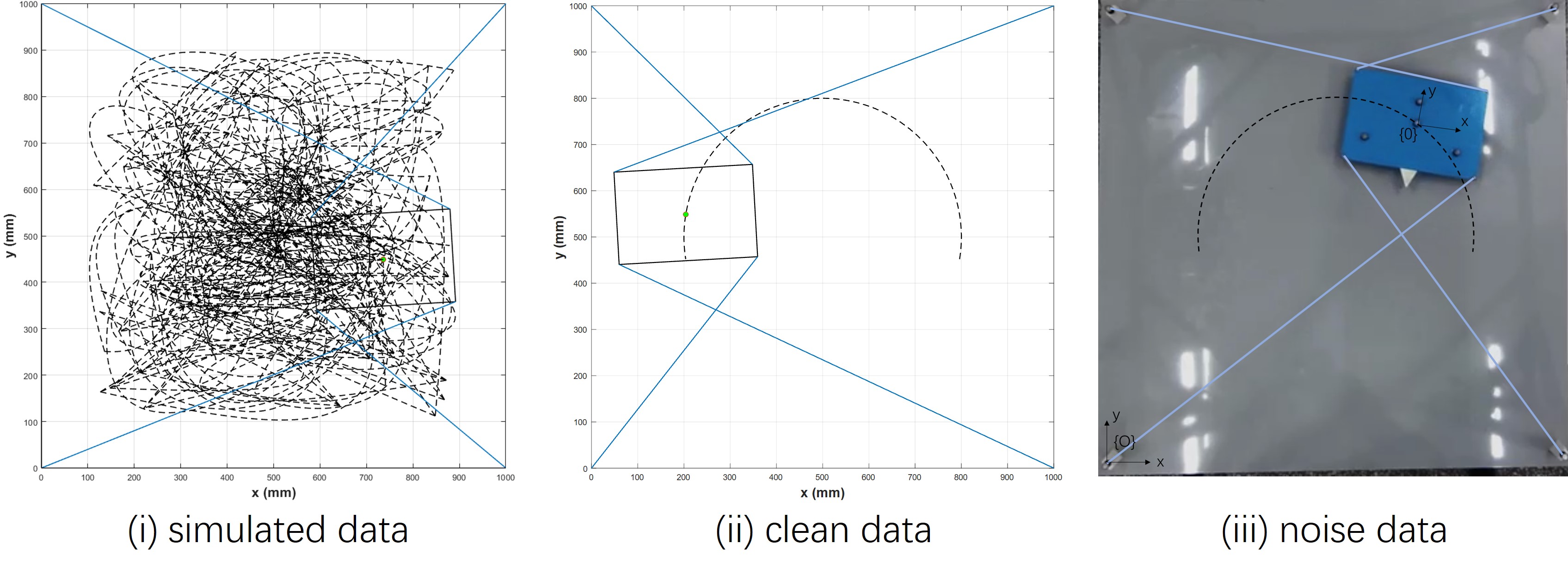
Figure 5: Data sources of Sim2Real experiment for the configuration of ExpC4. (i) Simulated data. In the simulator, there are $100$ random trajectories and $100$ samplings per trajectory. (ii) Clean data. In the simulator, we have devised a target trajectory with the objective of controlling the real CDPR to execute it. Here $1000$ samplings are generated. (iii) Noise data. In the real setup, the end-effector of CDPR follows the target trajectory. During the experiment, a total of 1103 data are collected. Above all, each data composes the end-effector pose ($x,y,\theta$) and the corresponding length of $4$ cables.

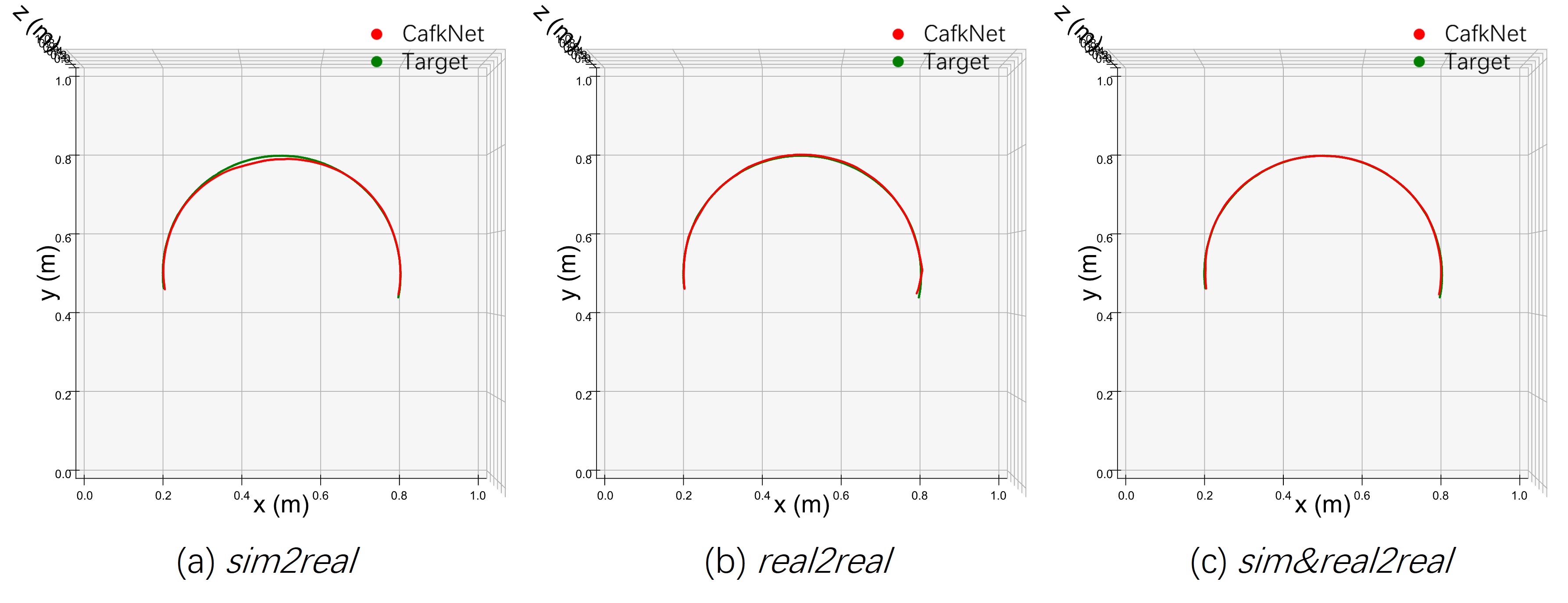
Figure 6: Target trajectory and resulting trajectory solved by CafkNet under three methods.

TABLE V: Sim2Real Experiment Details and Results. Cases i, ii, iii are revealed in Fig. 5. Bold: minimum error in each testing data.

Methods	Train on	Test on		Results (unit: mm)
		Clean Data	Noise Data	Clean Data	Noise Data
sim2real	i	ii	iii	1.7	1.6
real2real	$80\%$ ii	$20\%$ ii	iii	2.7	2.2
sim&real2real	$\text{i}+80\%$ ii	$20\%$ ii	iii	2.4	1.3

VII Conclusion

This paper presents CafkNet, a GNN-empowered FK solver for CDPRs. It is the first work to utilize GNNs for solving the FK problem in CDPRs. The study begins by introducing a graph structure that represents the topology of CDPRs. Subsequently, GNNs are employed to solve the FK problem by learning pose-length data. The experimental results demonstrate that CafkNet can learn the inherent topological relationships of CDPRs and accurately solve the FK issue. The results are validated across different types of CDPRs, including spatial CDPRs and planar CDPRs, as well as under various configurations such as under-constrained, fully-constrained, and over-constrained CDPRs. The validation is conducted in both simulation environments and real-world scenarios as well.

This work focuses solely on the FK problem, which is known to be challenging in the kinematic modeling of CDPRs. So, in the future, we aim to apply the GNN to solve the IK problem and dynamic modeling issues.

References

- [1] S. Qian, B. Zi, W.-W. Shang, and Q.-S. Xu, “A review on cable-driven parallel robots,” Chinese Journal of Mechanical Engineering, vol. 31, no. 1, pp. 1–11, 2018.
- [2] Z. Zhang, Z. Shao, Z. You, X. Tang, B. Zi, G. Yang, C. Gosselin, and S. Caro, “State-of-the-art on theories and applications of cable-driven parallel robots,” Frontiers of Mechanical Engineering, vol. 17, no. 3, p. 37, 2022.
- [3] M. Zarebidoki, J. S. Dhupia, and W. Xu, “A review of cable-driven parallel robots: Typical configurations, analysis techniques, and control methods,” IEEE Robotics & Automation Magazine, vol. 29, no. 3, pp. 89–106, 2022.
- [4] B. Zhang, W. Shang, X. Gao, Z. Li, X. Wang, Y. Ma, F. Zhang, R. Yao, H. Li, J. Yin, et al., “Synthetic design and analysis of the new feed cabin mechanism in five-hundred-meter aperture spherical radio telescope (fast),” Mechanism and Machine Theory, vol. 191, p. 105507, 2024.
- [5] A. Pott, “Forward kinematics and workspace determination of a wire robot for industrial applications,” Advances in Robot Kinematics: Analysis and Design, pp. 451–458, 2008.
- [6] C. B. Pham, S. H. Yeo, G. Yang, M. S. Kurbanhusen, and I.-M. Chen, “Force-closure workspace analysis of cable-driven parallel mechanisms,” Mechanism and Machine Theory, vol. 41, no. 1, pp. 53–69, 2006.
- [7] Z. Zhang, H. H. Cheng, and D. Lau, “Efficient wrench-closure and interference-free conditions verification for cable-driven parallel robot trajectories using a ray-based method,” IEEE Robotics and Automation Letters, vol. 5, no. 1, pp. 8–15, 2019.
- [8] B. Zhang, B. Deng, X. Gao, W. Shang, and S. Cong, “Design and implementation of fast terminal sliding mode control with synchronization error for cable-driven parallel robots,” Mechanism and Machine Theory, vol. 182, p. 105228, 2023.
- [9] A. Pott and V. Schmidt, “On the forward kinematics of cable-driven parallel robots,” in 2015 IEEE/RSJ International Conference on Intelligent Robots and Systems (IROS). IEEE, 2015, pp. 3182–3187.
- [10] U. A. Mishra and S. Caro, “Forward kinematics for suspended under-actuated cable-driven parallel robots with elastic cables: A neural network approach,” Journal of Mechanisms and Robotics, vol. 14, no. 4, p. 041008, 2022.
- [11] X. Wang, B. Zhang, W. Shang, and S. Cong, “Optimal reconfiguration planning of a 3-dof point-mass cable-driven parallel robot,” IEEE Transactions on Industrial Electronics, 2023.
- [12] Z. Zhang, “Ray-based interference free workspace analysis and path planning for cable-driven robots,” arXiv preprint arXiv:2211.07612, 2022.
- [13] Y. Liu, Z. Cao, H. Xiong, J. Du, H. Cao, and L. Zhang, “Dynamic obstacle avoidance for cable-driven parallel robots with mobile bases via sim-to-real reinforcement learning,” IEEE Robotics and Automation Letters, vol. 8, no. 3, pp. 1683–1690, 2023.
- [14] A. Akhmetzyanov, M. Rassabin, A. Maloletov, M. Fadeev, and A. Klimchik, “Model free error compensation for cable-driven robot based on deep learning with sim2real transfer learning,” in 17th International Conference on Informatics in Control, Automation and Robotics. Springer, 2022, pp. 479–496.
- [15] K. Wang, W. R. Johnson, S. Lu, X. Huang, J. Booth, R. Kramer-Bottiglio, M. Aanjaneya, and K. Bekris, “Real2sim2real transfer for control of cable-driven robots via a differentiable physics engine,” in 2023 IEEE/RSJ International Conference on Intelligent Robots and Systems (IROS). IEEE, 2023, pp. 2534–2541.
- [16] E. Ottaviano, M. Ceccarelli, and P. Pelagalli, “A performance analysis of a 4 cable-driven parallel manipulator,” in 2006 IEEE Conference on Robotics, Automation and Mechatronics. IEEE, 2006, pp. 1–6.
- [17] J.-P. Merlet, “Advances in the use of neural network for solving the direct kinematics of cdpr with sagging cables,” in International Conference on Cable-Driven Parallel Robots. Springer, 2023, pp. 30–39.
- [18] H. Hong, J. Ali, and L. Ren, “A review on topological architecture and design methods of cable-driven mechanism,” Advances in mechanical engineering, vol. 10, no. 5, p. 1687814018774186, 2018.
- [19] S. Zare, M. S. Haghighi, M. R. H. Yazdi, A. Kalhor, and M. T. Masouleh, “Kinematic analysis of an under-constrained cable-driven robot using neural networks,” in 2020 28th Iranian Conference on Electrical Engineering (ICEE). IEEE, 2020, pp. 1–6.
- [20] Y. Lu, S. Lin, G. Chen, and J. Pan, “Modlanets: learning generalisable dynamics via modularity and physical inductive bias,” in International Conference on Machine Learning. PMLR, 2022, pp. 14 384–14 397.
- [21] L. Yang, B. Huang, Q. Li, Y.-Y. Tsai, W. W. Lee, C. Song, and J. Pan, “Tacgnn: Learning tactile-based in-hand manipulation with a blind robot using hierarchical graph neural network,” IEEE Robotics and Automation Letters, vol. 8, no. 6, pp. 3605–3612, 2023.
- [22] S. Funabashi, T. Isobe, F. Hongyi, A. Hiramoto, A. Schmitz, S. Sugano, and T. Ogata, “Multi-fingered in-hand manipulation with various object properties using graph convolutional networks and distributed tactile sensors,” IEEE Robotics and Automation Letters, vol. 7, no. 2, pp. 2102–2109, 2022.
- [23] J. T. Kim, J. Park, S. Choi, and S. Ha, “Learning robot structure and motion embeddings using graph neural networks,” arXiv preprint arXiv:2109.07543, 2021.
- [24] A. Sanchez-Gonzalez, N. Heess, J. T. Springenberg, J. Merel, M. Riedmiller, R. Hadsell, and P. Battaglia, “Graph networks as learnable physics engines for inference and control,” in International Conference on Machine Learning. PMLR, 2018, pp. 4470–4479.
- [25] K. R. Allen, T. L. Guevara, Y. Rubanova, K. Stachenfeld, A. Sanchez-Gonzalez, P. Battaglia, and T. Pfaff, “Graph network simulators can learn discontinuous, rigid contact dynamics,” in Conference on Robot Learning. PMLR, 2023, pp. 1157–1167.
- [26] T. Wang, R. Liao, J. Ba, and S. Fidler, “Nervenet: Learning structured policy with graph neural networks,” in International conference on learning representations, 2018.
- [27] J. Whitman, M. Travers, and H. Choset, “Learning modular robot control policies,” IEEE Transactions on Robotics, 2023.
- [28] H. Sun, L. Yang, Y. Gu, J. Pan, F. Wan, and C. Song, “Bridging locomotion and manipulation using reconfigurable robotic limbs via reinforcement learning,” Biomimetics, vol. 8, no. 4, p. 364, 2023.
- [29] X. Ji, H. Li, Z. Pan, X. Gao, and C. Tu, “Decentralized, unlabeled multi-agent navigation in obstacle-rich environments using graph neural networks,” in 2021 IEEE/RSJ International Conference on Intelligent Robots and Systems (IROS). IEEE, 2021, pp. 8936–8943.
- [30] P. W. Battaglia, J. B. Hamrick, V. Bapst, A. Sanchez-Gonzalez, V. Zambaldi, M. Malinowski, A. Tacchetti, D. Raposo, A. Santoro, R. Faulkner, et al., “Relational inductive biases, deep learning, and graph networks,” arXiv preprint arXiv:1806.01261, 2018.
- [31] D. P. Kingma and J. Ba, “Adam: A method for stochastic optimization,” arXiv preprint arXiv:1412.6980, 2014.
- [32] R. Liaw, E. Liang, R. Nishihara, P. Moritz, J. E. Gonzalez, and I. Stoica, “Tune: A research platform for distributed model selection and training,” arXiv preprint arXiv:1807.05118, 2018.
- [33] P. Virtanen, R. Gommers, T. E. Oliphant, M. Haberland, T. Reddy, D. Cournapeau, E. Burovski, P. Peterson, W. Weckesser, J. Bright, et al., “Scipy 1.0: fundamental algorithms for scientific computing in python,” Nature methods, vol. 17, no. 3, pp. 261–272, 2020.