An Interior-Point Trust-Region Method for Nonsmooth Regularized Bound-Constrained Optimization
Abstract
We develop an interior-point method for nonsmooth regularized bound-constrained optimization problems. Our method consists of iteratively solving a sequence of unconstrained nonsmooth barrier subproblems. We use a variant of the proximal quasi-Newton trust-region algorithm TR of Aravkin et al. [2] to solve the barrier subproblems, with additional assumptions inspired from well-known smooth interior-point trust-region methods. We show global convergence of our algorithm with respect to the criticality measure of Aravkin et al. [2]. Under an additional assumption linked to the convexity of the nonsmooth term in the objective, we present an alternative interior-point algorithm with a slightly modified criticality measure, which performs better in practice. Numerical experiments show that our algorithm performs better than the trust-region method TR, the trust-region method with diagonal hessian approximations TRDH of Leconte and Orban [17], and the quadratic regularization method R2 of Aravkin et al. [2] for two out of four tested bound-constrained problems. On those two problems, our algorithm obtains smaller objective values than the other solvers using fewer objective and gradient evaluations. On the two other problems, it performs similarly to TR, R2 and TRDH.
keywords:
Regularized optimization, nonsmooth optimization, nonconvex optimization, bound constraints, proximal gradient method, barrier method.49J52, 65K10, 90C53, 90C56,
1 Introduction
We consider the problem
| (1) |
where has Lipschitz-continuous gradient with constant and is proper and lower semi-continuous. Both and may be nonconvex. is often considered as a regularization function used to favor solutions with desirable properties, such as sparsity.
Problems such as (1) are classically solved with a variant of the proximal gradient method [19]. The proximal quasi-Newton trust-region algorithm of Aravkin et al. [2], referred to as TR, can be extended to box constraints, provided that the proximal operator of , where componentwise and is the indicator of the box , can be computed efficiently. Leconte and Orban [17] present a variant of TR named TRDH that also supports box constraints, and uses diagonal quasi-Newton approximations. For specific separable regularizers , they provide a closed-form solution of the trust-region subproblems with box constraints, giving rise to what they defined as an indefinite proximal operator; a scaled generalization of a proximal operator.
At each iteration , we solve the barrier subproblem
| (2) |
where is the logarithmic barrier function
| (3) |
and . Each subproblem (2) is an unconstrained problem if we consider that when . In Section 5.2, we explain that under reasonable assumptions, we can solve solve (2) with a modified version of Aravkin et al.’s TR algorithm, and we expect that the solutions of (3) converge to a solution of (1) as .
Our approach is sometimes referred to as a trust-region interior-point method, or trust-region method for barrier functions. We refer the reader to [9, Chapter ] for more information on the case where . Our algorithm, named RIPM (Regularized Interior Proximal Method), can be seen as a generalization of those methods to solve (1).
An inconvenient of solving (2), induced by the logarithmic barrier function (3), is that the smooth part of the subproblem does not have a Lipschitz gradient, thus compromising the convergence properties of TR established by Aravkin et al. [2]. Nevertheless, in our analysis, we establish the convergence of the barrier subproblems using the update rules of Conn et al. [9, Chapter ] for our trust-region model. We also show global convergence of RIPM towards a first-order stationary point of (1) if the trust-region radii and the step lengths used in proximal operator evaluations are bounded away from zero, and the iterates generated by the algorithm remain bounded. In Section 5.4, under a convexity assumption on the nonsmooth term, we provide an alternative implementation of the outer iterations of RIPM where we change the stopping criteria to improve numerical performance.
In addition, we implement a variant of RIPM named RIPMDH (Regularized Interior Proximal Method with Diagonal Hessian approximations) that uses TRDH to solve the barrier subproblems. We compare the performance of RIPM and RIPMDH with TR, TRDH and R2, all available from RegularizedOptimization.jl [5], on four bound-constrained problems. The first two problems are a regularized box-constrained quadratic problem, and a sparse nonnegative matrix factorization problem. These two problems require many TR and R2 iterations to converge. RIPM and RIPMDH obtain smaller objective values than the other solvers using fewer objective and gradient evaluations, which suggests that they may be best suited to solve difficult bound-constrained nonsmooth problems. The third problem is an inverse problem for finding the parameters of a differential equation. RIPM and RIPMDH perform more objective and gradient evaluations than TR, but RIPMDH performs the least amount of proximal operator evaluations. The last problem is a regularized box-constrained basis-pursuite denoise problem. RIPMDH exhibits similar performance to those of TR, TRDH and R2 using a modification of some of its parameters.
Related research
Attouch and Wets [4] use and the nonsmooth barrier . They use the theory of epi-convergence to explain some convergence properties of barrier methods, and in particular, that the objectives of the barrier subproblems epi-converge to the objective of their initial constrained problem.
Chouzenoux et al. [7] use convex and with general inequality constraints for , to solve large-scale image processing problems. Their algorithm uses proximal gradient steps to solve the barrier subproblem.
Bertocchi et al. [6] solve inverse problems , where is some observed data, the signal to determine, is a linear observation operator, and is an operator applying noise perturbation. They solve the problem with constraints , where is a convex function involving the observations and the signal , and are twice differentiable, and are convex (among other properties). They compute the proximal operator of the barrier term, and use an interior-point algorithm. They apply their algorithm to develop a neural network architecture for image restoration.
De Marchi and Themelis [11] use the proximal gradient method to solve nonsmooth regularized optimization problems such as (1) where has a locally Lipschitz-continuous gradient, is continuous relative to its domain and prox-bounded. In addition, the constraint is replaced by a more general constraint , where has locally Lipschitz-continuous Jacobian.
Shen et al. [23] present an active set proximal algorithm to solve (1) with for some , and where with instead of . They use a hybrid search direction based upon a proximal gradient step for the active variables (i.e., the variables that are at one the bounds of the constraints), and a Newton step for the other variables.
Notation
For , denotes the Euclidean norm of . and , denote, respectively, the sets of positive and strictly positive real numbers, whereas and denote the sets of vectors having all their components in and , respectively.
denotes . The unit closed ball defined with the -norm and centered at the origin is , and the ball centered at the origin of radius is . If , the indicator of is defined by if , and if . For , the set is composed of all the vectors such that with .
Following the notation of Rockafellar and Wets [22], the set of all subsequences of is denoted by , and the set composed of the subsequences of containing all beyond some is denoted by . For , indicates that the subsequence (which we may also write for conciseness) converges to .
, and (possibly with subscripts, or) denote the square diagonal matrices having , and as diagonal elements, respectively.
2 Background
The following are standard variational analysis concepts—see, e.g., [22]. Let and where is finite. The Fréchet subdifferential of at is the closed convex set of elements such that
The limiting subdifferential of at is the closed, but not necessarily convex, set of elements for which there exist and such that and for all . The inclusion always holds. Finally, the horizon subdifferential of at is the closed, but not necessarily convex, cone of elements for which there exist , and such that , for all , and .
If , is the set of such that . For , is the set of such that .
If and , the closed convex cone is the regular normal cone to at . The closed cone is the normal cone to at . always holds, and is an equality if is convex.
If is convex, is the closed convex cone of elements such that for all [22, Theorem ].
For a set-valued mapping where, for any , , the graph of is the set .
For , the limit superior of at is , and the limit inferior of at is . and always hold.
The set-valued mapping is outer semicontinuous (osc) at if , or, equivalently, . It is inner semicontinuous (isc) at if , or equivalently when is closed-valued. If both conditions hold, is continuous at , i.e., as .
[22, Proposition ] For and where is finite, is osc at with respect to when , i.e. for any with , there exists for all such that .
The graphical outer limit of a sequence of set-valued mappings is defined by . The graphical inner limit of a sequence of set-valued mappings is defined by . If both limits agree, the graphical limit exists, so that we can also write , and we have .
The epigraph of is the set .
We denote the (lower) closure of , i.e., the largest function less than that is lower semi-continuous. Its epigraph is the closure of .
If for all , the lower and upper pointwise limits of are the functions and defined for all by
When and coincide, their common value is the pointwise limit of denoted . If , we write .
For a sequence , we define
Consider in particular . It is not difficult to see that and are also epigraphs in the sense that if is in either set, then so is for any . The lower epi-limit of is the function whose epigraph is , and the upper epi-limit of is the function whose epigraph is . It is always true that . When the two coincide, their common value is called the epi-limit of denoted . If , we also write .
The following result summarizes important properties of epi-limits used in the sequel.
[22, Proposition ] Let for .
-
1.
and are lsc, and so is when it exists;
-
2.
if for all , exists and equals ;
-
3.
if for al , exists and equals .
In addition, if , , with for all , and if and , then .
The model that we will use in our algorithm uses an approximation of at so that . For , the function-valued mapping is epi-continous at if as .
is level-bounded if, for every , the lower level set is bounded (possibly empty). The sequence of functions is eventually level-bounded if, for each , the sequence of sets is eventually bounded, i.e., there is an index set such that is bounded.
The following theorem establishes properties about the minimization of sequences of epi-convergent functions.
[22, Theorem ] Suppose the sequence is eventually level-bounded, and with and lsc and proper. Then,
| (4) |
with , while there exists such that is a bounded sequence of nonempty sets with
| (5) |
Indeed, for any and , is bounded and all its cluster points belong to . If consists of a unique point , one must actually have .
The proximal operator associated with the proper lsc function and parameter is
| (6) |
3 Stationarity
We say that the constraint qualification (CQ) holds at if contains no such that .
Our assumptions that is continuously differentiable and that is proper lsc allows us to write [22, Exercise and Theorem ]
Due to the simple form of , the constraint qualification states that the only such that and satisfying if is .
A simple example where the constraint qualification is not satisfied is found by setting , , and , i.e., if and , in (1). The unique solution is . Then, so that . The qualification condition requires that the only such that be , which is clearly not the case. Of course, the bound constraint in the example above is redundant and the constrained and unconstrained solutions coincide.
For fixed and , we define approximations
| (10a) | ||||
| (10b) | ||||
| (10c) | ||||
and the model of about
| (11) |
where . We point out that , which is the expression of the Lagrangian in the smooth case, thus, we use the superscript to denote objects sharing similarities with the smooth Lagrangian.
For , we further define
| (12a) | ||||
| (12b) | ||||
Our associated optimality measure is
| (13) |
where .
Let the CQ hold at , such that and . Then, is first-order stationary for (1).
Proof.
The first equivalence follows directly from (12b)–(13). The first-order necessary conditions for (12a) then imply
| (14) | ||||
As and are convex, so is . From this observation, we deduce that,
The CQ combined with the above equations indicate that there is no , such that , thus, [22, Corollary ] leads to
| (15) | ||||
By injecting (15) into (14), we obtain
From the observation above (9) and the fact that , we deduce that for any , . Thus,
4 Projected-directions methods
Let us briefly recall the proximal gradient method [19] used to solve
| (16) |
where has Lipschitz-continuous gradient and is proper and lower semi-continuous. The method generates iterates such that
| (17) |
where , which leads to the first-order stationarity conditions
| (18) |
A first approach to solving (1), that we can reformulate as
is to use projected-directions methods. A simple example of such methods consists in performing the identification in (16), and using the proximal gradient method as in (17).
Aravkin et al.’s TR and R2 are other examples of algorithms that can solve (1) with a similar strategy. Replacing by and by in all models of TR and R2 is sufficient to generalize these methods to (1), if a solution of
| (19) |
for TR, or
| (20) |
for R2, is available.
Leconte and Orban [17] implement a variant of TR named TRDH that handles bound constraints for separable regularizers (assuming that is also separable). TRDH solves at each iteration and for all the problem
| (21) |
with . The special choice shows that solving (21) for all is equivalent to solving (19).
However, for nonseperable regularizers , projected-directions methods rely on computing search directions such as (19), (20) or (21), which may be complicated (impossible for the latter), and therefore seems to be a limitation of this approach. The following section describes the implementation of a method that is different from projected directions methods, and is based upon interior-point techniques.
5 Barrier methods
Consider a sequence .
Let be defined as in (3). Then, .
Proof.
It is sufficient to show that for . Our goal is to bound each by two functions having as epi-limit. We define
By construction, , and as for all . In particular, and as .
By [22, Proposition c], because is nonincreasing with , its epi-limit is well defined and .
Similarly, by [22, Proposition d], because is nondecreasing with , its epi-limit is well defined and .
Because , [22, Proposition g] implies that , and consequently, we obtain .
.
Proof.
The following corollary legitimizes the barrier approach for (1).
Let be finite. For all ,
In particular, if ,
Proof.
Follows directly from [22, Theorem b].
If is finite, the definition of the limit superior of a sequence of sets and the second part of Section 5 indicate that for any , there exists and for all such that converges to a solution of (1).
5.1 Barrier subproblem
The -th subproblem is
| (22) |
is first-order stationary for (22) if
| (23) |
We call the process of solving (22) the -th sequence of inner iterations, and we denote its iterates for . The definition of (22) along with certain parameter updates will be called an outer iteration.
For and , let
| (24) |
Note that is closed, and also convex, as shown in the following lemma.
Let and . Then defined in (24) is convex.
Proof.
Let and , and . By definition, and . Now,
Thus, and is convex.
Under the assumptions of Section 5.1 and for , is convex.
At outer iteration , we choose , and solve (22) inexactly by approximately solving a sequence of trust-region subproblems of the form
| (25a) | ||||
| (25b) | ||||
where and model the smooth and nonsmooth parts of (22), respectively, and is a trust-region radius. Models are required to satisfy the following assumption.
Model Assumption 5.1.
For any and , is continuously differentiable on with and . In addition, is Lipschitz continuous with constant . We require that be proper, lsc, and satisfy and .
Let Model Assumption 5.1 be satisfied. Then is first-order stationary for (25) if and only if is first-order stationary for (22).
Proof.
If is first-order stationary, then . Note that so , and , so there is an open set such that for all , . Thus, using the definition of the subdifferential, . We conclude that , which is the definition of being first-order stationary for (25). The reciprocal can also be established from these observations, because if , we have shown that .
As a special case of Section 5.1, if solves (25), then is first-order stationary for (22).
Let
| (26) |
where , be a second order Taylor approximation of about . We are particularly interested in the quadratic model
| (27) | ||||
where is an approximation to the vector of multipliers for the bound constraints of (1).
Let be an approximate solution of (25). If is accepted as a step for our algorithm used to solve (22) (the acceptance condition is detailed in Algorithm 2), we perform the update .
By analogy with the smooth case, we use when is first-order stationary for (22). Multiplying through by , we obtain . Linearizing the continuous equality with respect to and and evaluating all quantities at iteration yields , which suggests that if , then .
However, the latter may not be positive. We perform the update described by Conn et al. [9], by defining
| (28) |
and projecting componentwise into the following interval to get
| (29) |
with . Projecting into (29) always generates a positive . The choice is also available. The other bounds of (29) will be useful in Section 5.2 and Section 5.3.
We define the following model, based upon a first-order Taylor approximation
| (30a) | ||||
| (30b) | ||||
where “cp” stands for “Cauchy point”. Let be the solution of (25) with model . As stated in [2, Section ], is actually the first step of the proximal gradient method (17) from applied to the minimization of with step length :
| (31) |
Let
| (32) |
where , and let be our measure of criticality. Aravkin et al. [2] and its corrigendum [1] indicate that is similar to , which is the norm of the generalized gradient at . We can apply [22, Theorems and ] to conclude that is proper lsc in . In particular, for any and solves (25), and is first-order stationary for (22).
Algorithm 1 summarizes the outer iteration.
For each outer iteration , the inner iterations generate a sequence according to an adaptation of [2, Algorithm ] in which the subproblems have the form (25) with the smooth part of the model defined by (27). Each trust-region step is required to satisfy the following assumption.
Step Assumption 5.1.
In Step Assumption 5.1, the subscript “m” of refers to the model adequacy, and the subscript “mdc” of refers to the model decrease.
Algorithm 2 summarizes the process.
5.2 Convergence of the inner iterations
Let and be fixed positive integers, and . We may rewrite our “Cauchy point” subproblem for the inner iterations as in [2]:
| (36a) | ||||
| (36b) | ||||
First, we present some properties of the subproblem (36a) in the following result.
[2, Proposition ] Let Model Assumption 5.1 be satisfied, , and . If we define and , the domain of and is . In addition,
-
1.
is proper lsc and for each , is nonempty and compact;
-
2.
if in such a way that , and for each , , then is bounded and all its limit points are in ;
-
3.
if is strictly convex, is single valued;
-
4.
if and there exists such that , then is continuous at and holds in part 2.
Proof.
Model Assumption 5.1 and the compactness of ensure that the objective of (36a) is always level-bounded in locally uniformly in , because for any , , and with , its level sets are contained in . From this observation, we can draw similar conclusions to the analysis of [2, Proposition ].
The observation in the proof of Section 5.2 and Model Assumption 5.1 allows us to derive directly some of the convergence properties of Aravkin et al. [2] for Algorithm 2.
[2, Theorem ] Let Model Assumption 5.1 and Step Assumption 5.1 be satisfied and let
| (37) |
If is not first-order stationary for (22) and , then iteration is very successful and .
Proof.
If is not first-order stationary, , thus and . The rest of the proof is identical to that of [2, Theorem ].
Now, let . Then, for all . If we consider defined in (27), for and in ,
| (38) |
As , if remains bounded, must be bounded away from zero to guarantee the existence of some such that for all . To apply the complexity results, and to establish that if is bounded below on , we need a stronger assumption on the Lipschitz constant of our model.
Model Assumption 5.2 (2, Model Assumption ).
In Model Assumption 5.1, there exists such that for all . In addition, we select in line 4 of Algorithm 2 in a way that there exists such that for all .
As in Aravkin et al. [2], we can set in Algorithm 2 to ensure if the first part of Model Assumption 5.2 holds with . The observations below (38) motivate us to prove that is bounded away from zero in the next result.
Let , Model Assumption 5.1 be satisfied for in (27), and . Then, there exists such that, for all , we have
| (39) |
Proof.
We proceed similarly as in Conn et al. [9, Theorem ]. Let be a positive integer and be a sequence generated by Algorithm 2. As is decreasing and , we have , which implies that (39) holds.
The following proposition shows that we can use the convergence results of Aravkin et al. [2] using the same assumptions they used for . It will justify that Model Assumption 5.2 can be used for defined in (27).
Under the assumptions of Section 5.2, let be defined as in (26) so that is Lipschitz continuous with constant and there exists such that for all . Then satisfies Model Assumption 5.2.
Proof.
We can use (29) and (39) to say that is bounded for all , and we deduce from (38) that satisfies Model Assumption 5.2.
Now, we justify that Step Assumption 5.1 holds when . As remains bounded away from with Section 5.2, so does by definition of . Since is Lipschitz-continuous,
| (40) |
and a second-order Taylor approximation of about gives
| (41) |
Under the assumptions of Section 5.2, , and
The above equality combined with (40) and (41) implies that (35a) holds.
To emphasize the similarities between our inner iterations and the trust-region algorithm of Aravkin et al. [2], and in light of Section 5.2, we use in our next results that satisfies Model Assumption 5.2, instead of writting assumptions on . The following proposition gives us a sufficient condition for (35b) to be satisfied.
[1, Proposition ] If Model Assumption 5.2 is satisfied with bounded Hessian approximations , then there exists such that (35b) holds for all .
Proof.
The proof is identical to that of [1, Proposition ] when replacing by , and using the subscripts where is the iteration number of the algorithm instead of the subscript.
Section 5.2 allows us to write the following convergence results for Algorithm 2. As in Aravkin et al. [2], we define the smallest iteration number such that
| (42) |
and we express the set of successful iterations, the set of successful iterations for which (42) has not yet been attained, and the set of unsuccessful iterations for which (42) has not yet been attained as
| (43a) | ||||
| (43b) | ||||
| (43c) | ||||
[2, Theorem ] Let Model Assumption 5.1 and Step Assumption 5.1 be satisfied. If Algorithm 2 only generates finitely many successful iterations, then for all sufficiently large and is first-order critical for (22).
Proof.
The proof is inspired from [2, Theorem ], which itself follows that of Conn et al. [9, Theorem ]. The assumptions indicate that there is such that all iterations are unsuccessful, and because of the update rules of Algorithm 2. We assume by contradiction that is not first-order critical. does not have any of its components equal to because it is attained after a finite number of iterations of Algorithm 2. As is proper, . Thus, Section 5.2 implies that there exists such that . Since all iterations are unsuccessful, there will be some such that , which implies that iteration is very successful with Section 5.2, and contradicts the fact that is not first-order critical.
Finally, we have the following result for the inner iterates. {shadyproposition}[2, Theorem ] Let , Model Assumption 5.1 and Model Assumption 5.2 be verified for defined in (27), and Step Assumption 5.1 be satisfied for Algorithm 2. If there are infinitely many successful iterations, then, either
| (44) |
Proof.
The proof is identical as that of [2, Theorem ].
Now, the definitions of in (30a) and as a minimizer of (25) with model indicate that
By reinjecting this inequality into the definition of in (32), we obtain
so that
| (45) |
From this observation, we deduce that in the following result. {shadylemma} If Model Assumption 5.1 holds for defined in (27) and
then .
Proof.
Now, we study the asymptotic satisfaction of the inner perturbed complementarity. We show that (34) is eventually satisfied, similarly to [9, Theorem ] in the smooth case.
Let , Model Assumption 5.1 and Model Assumption 5.2 be verified for defined in (27), Step Assumption 5.1 be satisfied for Algorithm 2, and for all . Then,
Proof.
We proceed similarly as in the proof of [9, Theorem ]. With the formula ,
Using Model Assumption 5.2, we have . This leads to with Equation 45, and we have that is bounded away from using Section 5.2. Therefore, either iteration is not successful and , or
Since is also bounded for all using Section 5.2 and (29), we have
| (46) |
For large enough, we have
| (47) |
so that if is large enough.
In Algorithm 1, each subproblem is solved approximately with tolerances and . This gives rise to the analysis in Section 5.3.
5.3 Convergence of the outer iterations
For each , the stopping condition of Algorithm 2 occurs in a finite number of iterations. Let denote the number of iterations performed by Algorithm 2 at outer iteration . To simplify the notation, let , , , and .
First, we present two assumptions that will be useful for our analysis.
Parameter Assumption 5.1.
To satisfy the second part of Parameter Assumption 5.1, we need to change in (27) to
| (48) | ||||
where with the taken componentwise and .
Since the results of Section 5.2 involving defined in (27) are all based upon Step Assumption 5.1, those results continue to apply if Step Assumption 5.1 holds for defined in (48). We now show that that is the case.
Fist, we observe that
Assume, as in Section 5.2, that . Since is bounded by definition, we use (40) and (41) to conclude that , and, if , (35a) holds. The proof of Model Assumption 5.2 is still valid when considering instead of , so that (35b) also holds. As a consequence, Step Assumption 5.1 still holds with defined in (48).
Now, our goal is to find a sequence such that . Under some additional assumptions on , this will allow us to establish that Algorithm 1 generates iterates that satisfy asymptotically (9). We begin with preliminary lemmas.
Proof.
The first step of the proximal gradient method satisfies (31). According to (18), its first-order optimality conditions are
| (50) |
As is not on the boundary of , there exists such that for all in an open ball of center and radius , . Thus, the definition of the subdifferential guarantees that
We know that using Section 5.1, and because is not on the boundary of . Therefore, (50) simplifies to
using Model Assumption 5.1 for .
The following assumption will be useful to establish that converges to zero sufficiently fast to guarantee the convergence of the outer iterations.
Parameter Assumption 5.2.
To justify that Parameter Assumption 5.2 is reasonable, assume for simplicity that is an index such that . We have
so that
and, if ,
We multiply the above inequality by to obtain
If , e.g., with , . Then, the choice guarantees that Parameter Assumption 5.2 is satisfied.
Let Model Assumption 5.1, Parameter Assumption 5.1 and Parameter Assumption 5.2 be satisfied, and for all , . Then, there exists such that for all , is not on the boundary of .
Proof.
For all , , thus Section 5.3 leads to . As a consequence, if , then is not on the boundary of . This is certainly true for sufficiently large, because in Parameter Assumption 5.1 and .
Now, we show that is not on the boundary of if is large enough. First, we point out that , because
Then, we have
| using Section 5.3 | ||||
and Parameter Assumption 5.2 indicates that . As , the inequality
| (52) |
is satisfied if is large enough, and
| (53) | by properties of the | |||||
Therefore, is not on the boundary of if is large enough. We conclude that there exists such that for all , is not on the boundary of .
Let Model Assumption 5.1, Parameter Assumption 5.1 and Parameter Assumption 5.2 be satisfied, and for all , . We define
| (54) |
Then, there exists a subsequence such that for all ,
| (55) |
and
| (56) |
Proof.
Section 5.3 indicates that there is a subsequence such that, for , is not on the boundary of . Thus, Section 5.3 holds, and
| (57) |
With defined in (54), we have (55). Now, for all , we use Section 5.2 to establish that
and, by summing the square of the above inequality for all ,
| (58) | ||||
so that . As and Parameter Assumption 5.2 holds, we deduce that .
Now, we present two assumptions on . The first will not be necessary for the remaining results of this subsection, except as one of the justifications for the second assumption. However, it will be used in Section 5.4.
Model Assumption 5.3.
is epi-continuous on .
Model Assumption 5.3 holds if is continuous on , but this condition is only sufficient, not necessary [22, Exercise ]. Let us consider the case where . Because is lsc, its epigraph is closed, thus the sequence of functions satisfies . Let and . [22, Exercise ] indicates that for and , . Since the latter is true for all , we conclude that Model Assumption 5.3 is satisfied.
Model Assumption 5.4.
For any sequences and such that for all ,
| (59) |
We present some cases for which Model Assumption 5.4 holds.
-
•
When . Attouch’s theorem [3] (also written in [22, Theorem ]) indicates that this condition is satisfied when and are proper, lsc, convex functions with (i.e., Model Assumption 5.3 holds). An extension to non-convex functions under some more sophisticated assumptions is established by Poliquin [21].
-
•
When and (e.g., ), using Section 2 applied to .
-
•
When but is not continuous, we may still be able to show that Model Assumption 5.4 holds. For example, with , [16, Theorem ] shows that . Thus, .
Under the assumptions of Section 5.3 and Model Assumption 5.4, let and be limit points of and , respectively. Then,
| (60) |
In this case, when the CQ is satisfied at , is first-order stationary for (1).
Proof.
In Section 5.3, can be chosen such that and . We apply Model Assumption 5.4 to (55) and (56) to deduce
| (61) |
which indicates that . The condition (34) implies that . When the CQ is satisfied, we can use Section 3 to conlude that is first-order stationary for (1).
In Section 5.3, evokes of the concept of -KKT optimality for interior-point methods introduced in [11, Definition ]. We slightly modify this concept in the following definition.
Definition 5.1.
Let , , and . is said to be -KKT optimal if there exist and such that
| (62) |
and, for all ,
| (63) |
The main modification to the original formulation in [11, Definition ] is that we require instead of for all , but this is linked to our different choices of stopping condition for the complementary slackness. The first part of the definition (62) is similar to the -stationarity [10, Definition ] for more general problems.
Model Assumption 5.1 does not necessarily guarantee that . Thus, for where is a subsequence introduced in Section 5.3, we cannot use Section 5.3 to measure the -KKT optimality of . Let
| (64) |
As Section 5.3 indicates that , we can obtain a measure of -KKT optimality which depends on . When all the elements of are close to an element of , we expect to be small. In particular, if , . {shadytheorem} Let the assumptions of Section 5.3 be satisfied, and be defined in (64). Then, there exists such that for all , is -KKT optimal with constants
Proof 5.2.
Section 5.3 guarantees that, for all in a subsequence , (55) holds, i.e.
where is defined in (54). As is closed, we can choose such that, for , we have . Then,
which we may rewrite as
and
Section 5.3 implies that . We combine the latter inequality with (56) in Section 5.3 to obtain
| (65) |
Now, for all ,
| (66) | ||||
We use (65), (66) and Definition 5.1 to conclude.
If is bounded, in Equation 64. If , we also have .
5.4 Convergence with a new criticality measure
Now, instead of using (involving ) for the criticality measure of Algorithm 2, we would like to use a measure based upon defined in (10a). The reason behind this choice is inspired from the criticality measure used in primal-dual trust region algorithms in the smooth case, instead of used in primal algorithms, see for example [9, Algorithm ]. We may expect that this choice results in fewer iterations of Algorithm 2 when and are close to a solution of (1), because (we express this idea with smooth notations for now), if is the index for which the stopping criteria of Algorithm 2 are met, , whereas . However, to change the stopping criterion, we need the following convexity assumption.
Model Assumption 5.5.
For a sequence generated by Algorithm 2 at iteration , is convex for all .
If and is convex, Model Assumption 5.5 holds.
In this section, we define
| (67) |
where is defined in (11), and
| (68) |
where is defined in (10a). We point out that and defined in (13) are almost identical, the latter being computed by replacing by in (67). Model Assumption 5.5 will be useful in Section 5.4, which is crucial for our analysis of Algorithm 3 because it establishes the convergence of the inner iterations with .
Algorithm 3 resembles Algorithm 1, except for the stopping criterion (33). Our ultimate goal in this subsection is to show that replacing (33) in Algorithm 1 by (69) in Algorithm 3 maintains similar convergence properties to those of Section 5.3, but, as illustrated in Section 6, performs better in practice.
The following result shows that the inner iteration terminates finitely.
Under the assumptions of Section 5.2, Model Assumption 5.3 and Model Assumption 5.5, if possesses a limit point , then
| (70) |
and
| (71) |
where is defined in (67).
Proof 5.3.
As and , there exists an infinite subsequence such that , , , and with Section 5.2 with . By continuity of the , . The sets and are convex (using Section 5.1 for the latter). Since and are convex and cannot be separated, we use [22, Theorem ] to conclude that
With [22, Theorem ], we deduce
Thanks to Section 5.2 and the smoothness of and , we also have
| (72) |
The functions , and are all convex because they are linear. Model Assumption 5.3 implies that . Model Assumption 5.5 and [22, Theorem ] lead to
| (73) |
and the above functions are all convex. We deduce from (72), (73) and [22, Theorem ] that
where is defined in (11). The sequences and are level-bounded because of the indicators. As in (31), we have
and the above problem is single valued because of [22, Theorem ]. Let denote its only solution. Section 2, and specifically (5), implies that the sequences
and
have the same limit . We have shown in Equation 45 that . Thus, . Finally, we have
As by Model Assumption 5.2, and , we deduce that
Using (4) in Section 2, we have
| (74) |
The expression of in (68) can also be written as
By injecting the limit of and (74) in the above equation, we obtain (70).
From this point on, denotes the number of iterations performed by Algorithm 2 at iteration with the inner stopping criteria from Algorithm 3, and we use again the notation , , , , , with the addition of . The following three lemmas are analogous to Section 5.3, Section 5.3 and Section 5.3.
Proof 5.4.
The first-order stationarity condition of (67) is
The same analysis as in the proof of Section 5.3 establishes that
so that (75) holds.
Proof 5.5.
Let Model Assumption 5.1, Parameter Assumption 5.1 and Parameter Assumption 5.2 be satisfied, and for all , . Then, there exists such that for all , is not on the boundary of .
Proof 5.6.
Since for any , , Section 5.4 leads to . Thus, if , is not on the boundary of . As in Parameter Assumption 5.1 and , this is true if is sufficiently large. The rest of the proof is identical to that of Section 5.3.
Now, we can establish results similar to Section 5.3, Section 5.3, and Equation 64 for Algorithm 3.
Let Model Assumption 5.1, Parameter Assumption 5.1 and Parameter Assumption 5.2 be satisfied, and for all , . Then, there exists a subsequence such that for all ,
| (77) |
with
| (78) |
Proof 5.7.
Section 5.4 and Section 5.4 lead to (77). Section 5.4 shows that , and, as , (78) is satisfied.
Under the assumptions of Section 5.4 and Model Assumption 5.4, let and be limit points of and , respectively. Then,
| (79) |
In this case, when the CQ is satisfied, is first-order stationary for (1).
Proof 5.8.
In Section 5.4, can be chosen such that and . We apply Model Assumption 5.4 to (77) and (78) to obtain
and we conclude as in the proof of Section 5.3.
Finally, we show a result similar to Equation 64 for the -KKT optimality. We use again a subsequence as in section 5.4, , and we define
| (80) |
Let the assumptions of Section 5.4 be satisfied, and be defined in (80). Then, there exists a subsequence such that for all , is -KKT optimal with constants
Proof 5.9.
Section 5.4 guarantees that there exists an infinite subsequence such that for all ,
Since is closed and nonempty, we can choose such that, for , we have . Now,
which can also be written as
The triangle inequality combined and the Lipschitz constant of leads to
Section 5.4 then implies that
Finally, the inequalities of (66) still hold when replacing by : for all , .
When and , is bounded, thus in Section 5.4. If , we also have .
6 Implementation and numerical experiments
All solvers tested are available from RegularizedOptimization.jl. We define
where is a predefined relative tolerance for the inner iterations. Algorithm 2 terminates when
We use the constant for in (48) and . We set , , , and , similarly as Conn et al. [8] did in the smooth case for their interior-point trust-region algorithm. In addition, we go to iteration and set if Algorithm 2 performs more than iterations. Any iteration where is not first-order stationary for (1) has , thus the remarks below Parameter Assumption 5.2 are not sufficient to prove that this assumption is always satisfied, however, we observe satisfying performance with these parameters. Although it is possible to use , it would require more inner iterations.
To declare convergence of Algorithm 3, we use the following criteria
| (81a) | ||||
| (81b) | ||||
| (81c) | ||||
where , for some . In our experiments, we chose . We could not base our criteria upon in (13) because we do not know the associated to this measure (which is different from the generated by Algorithm 2 associated to the barrier subproblem).
Once Algorithm 3 terminates, we use a crossover technique to set or/and , to respect the complementarity condition. To do so, we check the final value of (resp. ), and if it is smaller than we set it to zero. If both and are smaller than , we set them to zero.
The subproblems in Algorithm 3 are solved with the algorithm R2 [2], and we compare Algorithm 1 to TR [2] with R2 used as a subsolver, and R2 used by itself. Algorithm 3 will be denoted RIPM. Finally, we introduce a variant of RIPM named RIPMDH (Regularized Interior Proximal Method with Diagonal Hessian approximations), that uses the same idea as our algorithm TRDH [17]: instead of using LBFGS or LSR1 quasi-Newton approximations for , we use diagonal quasi-Newton approximations so that (25) with defined in (48) can be solved analytically for specific seperable regularizers . TRDH and RIPMDH use the Spectral Gradient update in all our results. We choose either or , where . When , RIPM and RIPMDH denote Algorithm 1 instead of Algorithm 3 because is not convex.
For simplicity, we described how to solve (1) with the constraint , but RIPM and RIPMDH are actually able to handle box constraints . These more general constraints can be handled with minor modifications using the barrier function
| (82) |
instead of [9, Section ]. When (resp. ) for some , we remove the term (resp. ) from the first (resp. second) sum in (82).
Our results report
-
•
the final ;
-
•
the final , where is a parameter relative to our regularization function ;
-
•
the final stationarity measure ;
-
•
, where is the exact solution, if it is available;
-
•
the number of smooth objective evaluations ;
-
•
the number of gradient evaluation ;
-
•
the number of proximal operator evaluations ;
-
•
the elapsed time in seconds.
Our main goal is to reduce the number of objective and gradient evaluation, as they are typically costly to evaluate. Since we did not fully optimize the allocations in our algorithms, we do not pay attention to the elapsed time, and we only report it in the tables for information.
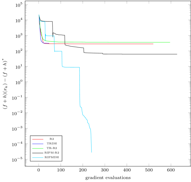
Once a problem has been solved by all solvers, we compare their final objective values and we save the smallest, that we denote . Then, for all solvers, we plot for every iteration where the gradient is evaluated. This allows us to represent the evolution of the objective per gradient evaluation. For the last gradient evaluation of RIPM and RIPMDH, we display their final objective value after applying the crossover technique.
6.1 Box-constrained quadratic problem
For our first numerical experiment, we solve
| (83) |
which is similar to [23, Section ], where , , has nonzero components with probability following a normal law of mean and standard deviation , has components generated using a normal distribution of mean and standard deviation , and , with , are vectors sampled from a uniform distribution between and . We chose , and use a LSR1 quasi-Newton approximation for TR and RIPM. For , the components of the solutions returned by TR, TRDH, R2, RIPM and RIPMDH satisfy for almost all . In this case, we observe that TR, TRDH and R2 are more efficient than RIPM. However, as we decrease , we get more components . We show results with in Figure 1 and Table 1. TRDH performs the least amount of objective, gradient and proximal operators evaluations. RIPMDH finds the smallest final objective value, and performs fewer objective, gradient and proximal operator evaluations than TR-R2. RIPM terminates with a criticality measure higher than the other solvers, but we observe that its final objective is smaller than those of TR, TRDH and R2. For RIPM and RIPMDH, we can clearly see plateaus that delimit the outer iterations. RIPM-R2 performs many more proximal operator evaluations than RIPMDH, because it uses up to R2 iterations to solve (25). The number of proximal operator evaluations with RIPM-R2 is also much higher than that of TR-R2, because the subproblems solved with R2 in RIPM-R2 have their objective based upon (48), which is not well conditioned when some components of approach , whereas the subproblems in TR-R2 are based upon (26).
| solver | () | ||||||
|---|---|---|---|---|---|---|---|
| R2 | e | e | e | e | |||
| TRDH | e | e | e | e | |||
| TR-R2 | e | e | e | e | |||
| RIPM-R2 | e | e | e | e | |||
| RIPMDH | e | e | e | e |
6.2 Sparse nonnegative matrix factorization (NNMF)
The second experiment considered is the sparse nonnegative matrix factorization (NNMF) problem from Kim and Park [15]. Let have nonnegative entries. Each column of represents an observation, and is generated using a mixture of Gaussians where negative entries are set to zero. We factorize by separating into clusters, where , both have nonnegative entries and is sparse. This problem can be written as
| (84) |
where and stacks the columns of to form a vector.
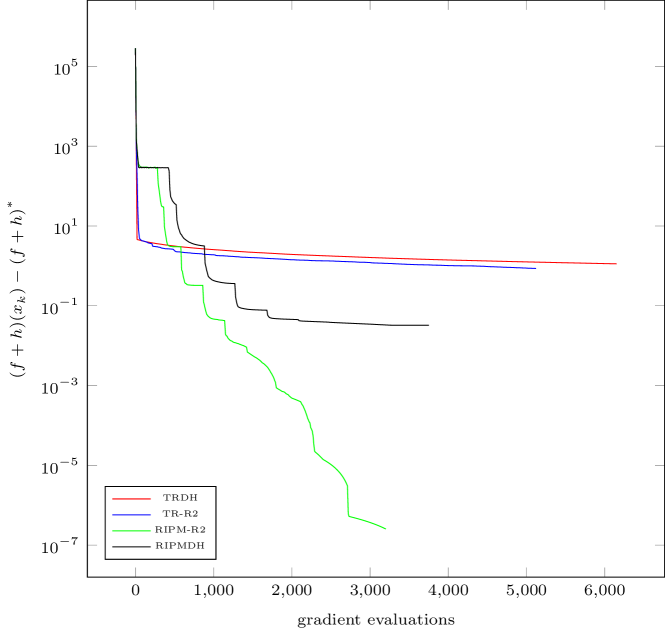
We set , , , , and report the statistics in Table 2. For this particular problem, we use , which allows for more accurate solves and for a better visualization of the evolution of the objective values, shown in Figure 2. We observe that RIPM-R2 and RIPMDH are the only solvers to terminate. They outperform R2 and TR-R2 in terms of number of objective and gradient evaluations, and their final objective value is also smaller. R2 and TR-R2 reach the maximum number of iterations. The objective of RIPM-R2 and RIPMDH is higher than that of R2 and TR-R2 only in the early iterations, because the barrier function has more effect when is larger. RIPM-R2 performs less objective and gradient evaluations than RIPMDH, but much more proximal operator evaluations because of the reasons evoked in Section 6.1.
| solver | () | ||||||
|---|---|---|---|---|---|---|---|
| TRDH | e | e | e | e | |||
| TR-R2 | e | e | e | e | |||
| RIPM-R2 | e | e | e | e | |||
| RIPMDH | e | e | e | e |
6.3 FitzHugh-Nagumo problem (FH)
We sample the functions and satisfying the FitzHugh [13] and Nagumo et al. [20] model for neuron activation, where , as and .
| (85) |
The time interval is discretized, with the initial conditions . We solve
| (86) |
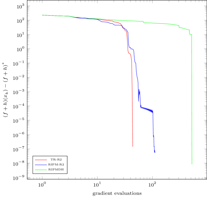
where with , , and report the statistics in Table 3. Since is not convex, we use Algorithm 1 instead of Algorithm 3. We do not show results with R2 because it encounters a numerical error during the solve of a differential equation to compute the objective. The evolution of the objective per gradient evaluation is shown in Figure 3. To improve readability, we choose to show the number of gradient evaluations on a logarithmic scale, and not to plot results with TRDH. All solvers converge to the value except for TRDH that has a higher final objective value than the other solvers. TR-R2 is the fastest, and seems the most suited to solve smaller problems such as (86). RIPM and RIPMDH still converge, but the latter is much slower. However, RIPMDH performs the least amount of proximal operator evaluations.
| solver | () | ||||||
|---|---|---|---|---|---|---|---|
| TRDH | e | e | e | ||||
| TR-R2 | e | e | e | ||||
| RIPM-R2 | e | e | e | ||||
| RIPMDH | e | e | e |
6.4 Constrained basis pursuit denoise (BPDN)
We solve the basis pursuit denoise problem (BPDN) [24, 12] with additional bound constraints. Let , , , where , has orthonormal rows, and is a vector of zeros, except for of its components that are set to . The constrained BPDN problems is written as
| (87) |
where . We use .
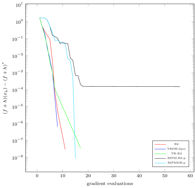
The statistics are shown in Table 4. R2, TRDH and TR-R2 are much more efficient than RIPM on this problem. This could come from the fact that there are many active bounds in the solution. However, this was also the case for the NNMF problem of Section 6.2, for which RIPM seems more efficient. Further investigations should seek to understand such behaviours on different problems. RIPM-R2-p and RIPMDH-p use the modifications and , which make RIPMDH on (87) surpass TR-R2 and close to TRDH. Figure 4 shows the evolution of the objective values. RIPM and RIPMDH are not included to improve readability.
| solver | () | |||||||
|---|---|---|---|---|---|---|---|---|
| R2 | e | e | e | e | e | |||
| TRDH | e | e | e | e | e | |||
| TR-R2 | e | e | e | e | e | |||
| RIPM-R2 | e | e | e | e | e | |||
| RIPMDH | e | e | e | e | e | |||
| RIPM-R2-p | e | e | e | e | e | |||
| RIPMDH-p | e | e | e | e | e |
7 Discussion and future work
We have presented RIPM, a trust-region interior-point method to solve nonsmooth regularized problems with box constraints, and RIPMDH, a variant based upon techniques of Leconte and Orban [17]. These algorithms solve a sequence of unconstrained barrier subproblems to obtain a sequence of approximate solutions of (1). We have shown the convergence of the inner barrier subproblems, and we have characterized the degree of -KKT optimality for every outer iteration past a certain rank. Under the assumption that the iterates remain bounded, we have shown that RIPM converges to a first-order stationary point for (1). We compared RIPM and RIPMDH to projected-direction methods with a separable regularization function.
RIPM and RIPMDH perform well on the box-constrained quadratic problem of Section 6.1 and on the NNMF problem of Section 6.2. They are not as efficient on the FH problem of Section 6.3 and the constrained BPDN problem of Section 6.4, which may suggest that projected-direction methods may be more efficient to solve problems with fewer variables and constraints. However, as observed with RIPM-R2-p and RIPMDH-p, the modification of two parameters of RIPM and RIPMDH improves their efficiency significantly on the constrained BPDN problem. This suggests that our implementation could benefit from parameter tuning.
Future work may include generalizing the algorithm to constraints of the form with for some , where the are continuously differentiable and Lipschitz-gradient continuous, as in [9, Section ] in the smooth case, or [11] for nonsmooth problems.
Another improvement would be to scale the trust region to allow greater search directions along the boundary of the feasible domain. This is explained more in detail in [9, Section ] for trust-regions based upon the -norm. However, we could not find an alternative for trust-regions based upon the -norm that led to satisfying numerical results.
In Section 5.4, Model Assumption 5.5 does not allow the use of with Algorithm 3. It would be interesting to see whether it is possible to establish convergence properties similar to those of Algorithm 1 without this assumption. One way to do this might be to replace by in (35b) when is large enough, but we did not manage to justify that this change results in a reasonable Step Assumption 5.1.
The extension of the convergence results to locally Lipschitz-gradient continuous functions could also be studied, based upon the work of [10, 11, 14].
Finally, when grows unbounded, we may still be able to prove the convergence of RIPM using the analysis of Leconte and Orban [18], provided that the norm of the Hessian approximations do not grow too fast.
References
- Aravkin et al. [2023] A. Aravkin, R. Baraldi, G. Leconte, and D. Orban. Corrigendum: A proximal quasi-Newton trust-region method for nonsmooth regularized optimization. Les Cahiers du GERAD G-2021-12-SM, Groupe d’études et de recherche en analyse des décisions, GERAD, Montréal QC H3T 2A7, Canada, Aug. 2023.
- Aravkin et al. [2022] A. Y. Aravkin, R. Baraldi, and D. Orban. A proximal quasi-Newton trust-region method for nonsmooth regularized optimization. SIAM J. Optim., 32(2):900–929, 2022.
- Attouch [1977] H. Attouch. Convergence de fonctions convexes, des sous-différentiels et semi-groupes associés. CR Acad. Sci. Paris, 284(539-542):13, 1977.
- Attouch and Wets [1981] H. Attouch and R. J.-B. Wets. Approximation and convergence in nonlinear optimization. In O. L. Mangasarian, R. R. Meyer, and S. M. Robinson, editors, Nonlinear Programming 4, pages 367–394. Academic Press, 1981. ISBN 978-0-12-468662-5.
- Baraldi et al. [2022] R. Baraldi, G. Leconte, and D. Orban. RegularizedOptimization.jl: Algorithms for regularized optimization. https://github.com/JuliaSmoothOptimizers/RegularizedOptimization.jl, February 2022.
- Bertocchi et al. [2020] C. Bertocchi, E. Chouzenoux, M.-C. Corbineau, J.-C. Pesquet, and M. Prato. Deep unfolding of a proximal interior point method for image restoration. Inverse Problems, 36(3):034005, feb 2020.
- [7] E. Chouzenoux, M.-C. Corbineau, and J.-C. Pesquet. A Proximal Interior Point Algorithm with Applications to Image Processing. J. Math. Imaging Vis., 62(6):919–940.
- Conn et al. [2000a] A. R. Conn, N. I. M. Gould, D. Orban, and P. L. Toint. A primal-dual trust-region algorithm for non-convex nonlinear programming. Math. Program., 87(2):215–249, 2000a.
- Conn et al. [2000b] A. R. Conn, N. I. M. Gould, and Ph. L. Toint. Trust-Region Methods. Number 1 in MOS-SIAM Series on Optimization. SIAM, Philadelphia, USA, 2000b.
- [10] A. De Marchi and A. Themelis. Proximal Gradient Algorithms Under Local Lipschitz Gradient Continuity. J. Optim. Theory and Applics., 194(3):771–794.
- De Marchi and Themelis [2024] A. De Marchi and A. Themelis. An interior proximal gradient method for nonconvex optimization. arXiv preprint 2208.00799, 2024.
- Donoho [2006] D. Donoho. Compressed sensing. IEEE T. Inform. Theory, 52(4):1289–1306, 2006.
- FitzHugh [1955] R. FitzHugh. Mathematical models of threshold phenomena in the nerve membrane. B. Math. Biophys., 17(4):257–278, 1955.
- Kanzow and Mehlitz [2022] C. Kanzow and P. Mehlitz. Convergence Properties of Monotone and Nonmonotone Proximal Gradient Methods Revisited. J. Optim. Theory and Applics., 195(2):624–646, 2022.
- Kim and Park [2008] J. Kim and H. Park. Sparse nonnegative matrix factorization for clustering. Technical Report GT-CSE-08-01, Georgia Inst. of Technology, 2008.
- Le [2013] H. Y. Le. Generalized subdifferentials of the rank function. Optimization Letters, 7(4):731–743, 2013.
- Leconte and Orban [2023a] G. Leconte and D. Orban. The indefinite proximal gradient method. Les Cahiers du GERAD G-2023-37, Groupe d’études et de recherche en analyse des décisions, GERAD, Montréal QC H3T 2A7, Canada, Aug. 2023a.
- Leconte and Orban [2023b] G. Leconte and D. Orban. Complexity of trust-region methods with unbounded Hessian approximations for smooth and nonsmooth optimization. Les Cahiers du GERAD G-2023-65, Groupe d’études et de recherche en analyse des décisions, GERAD, Montréal QC H3T 2A7, Canada, Dec. 2023b.
- Lions and Mercier [1979] P.-L. Lions and B. Mercier. Splitting algorithms for the sum of two nonlinear operators. SIAM J. Numer. Anal., 16(6):964–979, 1979.
- Nagumo et al. [1962] J. Nagumo, S. Arimoto, and S. Yoshizawa. An active pulse transmission line simulating nerve axon. Proceedings of the IRE, 50(10):2061–2070, 1962.
- Poliquin [1992] R. A. Poliquin. An extension of Attouch’s theorem and its application to second-order epi-differentiation of convexly composite functions. Transactions of the American Mathematical Society, 332:861–874, 1992.
- Rockafellar and Wets [1998] R. Rockafellar and R. Wets. Variational Analysis, volume 317. Springer Verlag, 1998.
- Shen et al. [2020] C. Shen, W. Xue, L.-H. Zhang, and B. Wang. An Active-Set Proximal-Newton Algorithm for Regularized Optimization Problems with Box Constraints. Journal of Scientific Computing, 85(3):57, 2020.
- Tibshirani [1996] R. Tibshirani. Regression shrinkage and selection via the lasso. J. Roy. Statist. Soc. Ser. B, 58(1):267–288, 1996.