Hy-DAT: A Tool to Address Hydropower Modelling Gaps Using Interdependency, Efficiency Curves, and Unit Dispatch Models

Abstract

As the power system continues to be flooded with intermittent resources, it becomes more important to accurately assess the role of hydro and its impact on the power grid. While hydropower generation has been studied for decades, dependency of power generation on water availability and constraints in hydro operation are not well represented in power system models used in the planning and operation of large-scale interconnection studies. There are still multiple modeling gaps that need to be addressed; if not, they can lead to inaccurate operation and planning reliability studies, and consequently to unintentional load shedding or even blackouts. As a result, it is very important that hydropower is represented correctly in both steady-state and dynamic power system studies. In this paper, we discuss the development and use of the Hydrological Dispatch and Analysis Tool (Hy-DAT) as an interactive graphical user interface (GUI), that uses a novel methodology to address the hydropower modeling gaps like water availability and inter-dependency using a database, and algorithms, to generate accurate representative models for power system simulation.

I Introduction

In the evolving power system, where new renewable resources displace continually conventional generation and hydro becomes a single traditional resource that is fully controllable, it is timely to examine hydropower generation’s role in the power system of the future and its representation in power system operation and planning reliability studies. Energy generation through hydroelectricity has a vital role in the development of a region and its economy. Hydropower generation depends on a lot of external factors such as water availability due to annual precipitation and snow water melting as a result representing hydropower generation accurately in electrical power system models requires proper translation of hydrology into the electrical capability of the plants. As the renewable generation penetration continues to increase, hydropower operation has evolved from a base load resource to a regulating resource. As a result, it is very important that hydropower is represented correctly in both steady-state and dynamic power system studies [1]. These gaps in hydropower modeling are mainly a consequence of decoupling hydro conditions and hydro-based constraints with electrical models used in steady-state and dynamic studies [2, 3]. The following gaps have been identified in close collaboration with the industry:

• Water availability in steady-state and dynamic models are not properly represented.

• Inter-dependencies among hydro projects in the same river systems are not properly represented.

• Environmental constraints are not represented in models.

• Rough zones are not represented in the power system model so generation dispatch in system studies might not be realistic.

• Many outdated dynamic models of hydropower generation turbines are still in use.

In order to conduct more accurate planning and operation studies, and ensure the grid operates reliably, it is vital to more accurately model hydropower generation. In this paper, we present the development of a tool that helps to address the hydropower modeling gaps with respect to water availability and inter-dependencies through the usage of databases and specific tools to translate historical hydrology into representative models that can be used in major power system simulations. The paper has the following sections: Section II provides the database components and features essential for the tool development, Section III provides an insight into the application of database for various tools like the efficiency curve estimation, inter-dependency evaluation using historical datasets, and the regression mode used for unit-level dispatch of hydropower resources to be integrated with Hy-DAT. Section IV provides an integration of the various features for power system model updates and a reference case study. Finally, Section V concludes the paper with some discussions and future work.

II Database Generation and Utilization

One of the major objectives of this work is to couple the historical hydro data available in the literature [4], [5] with the electrical data. The unit level generation dispatch data obtained from the Supervisory Control and Acquisition Data (SCADA) measurements are taken as an Energy Management system (EMS) snapshot of the system operating condition that can be utilized in the various planning cases considered in this work. This hydro data and the electrical data for various plants and units considered in this work has been uploaded to the Database Management System (DBMS), DB Browser [6] software tool using the structured query language (SQL) libraries utilized through various python scripts developed as part of this work.

II-A Source, Structure and Data Description

The timeseries hydro data, unit level MW dispatch data, for this work, that has been populated in to the database has been divided into six sections whose details has been presented below:

• ’Plant_Data’: The hydro data, in this work, is a timeseries data comprising of 10 years of data (2013-2023) with a sampling frequency of 1hr, for various hydro plants across the Columbia River Basin [4].

• ‘Unit_Data’: This table has been populated with the electrical data obtained using TSAT [7] tool (to convert the EMS data obtained from SCADA to capture the unit level dispatch data).

• ‘Static_Plant_Data’: This table contains plant level data, obtained from a 2020 Western Electricity Coordinating Council (WECC) summer planning case and [8]. This table contains the location based data such as latitude, longitude and area number of the plant and generic hydro based data such as head value of the plant.

• ‘Static_Unit_Data’: Similar to the ‘Static_Plant_Data’ table, this table contains unit level static data.

• ‘Efficiency_Raw_Data’: This table contains the calculated efficiencies for each individual generation units using the flow data from the ‘Plant_Data’ table.

• ‘Efficiency_Estimated_Data’: The hydro data for the plants is not available throughout the operating range of a generation unit to account for its electrical power output. Therefore, a linear regression model has been developed to extrapolate the missing estimated flow and estimated electrical power values for the individual units.

II-B Database Schema and Database Instances

The database schema developed in this work has been linked with each other using a common identifier as shown in Table I. This method of linking the tables using a common column identifier becomes important during the GUI development process of this work as discussed in Section IV-C of this work.

TABLE I: Subset Classification of Tables based on the considered common column identifiers

Subset	Column Identifier Name	Tables
1	Project_Name	Plant_Data, Unit_Data, Static_Unit_Data, Static_Plant_Data
2	Unit_ID	Efficiency_Raw, Efficiency_Estimated

In Table I, it should be noted that the tables in Subset 2 are linked to the tables in Subset 1 through the ‘Unit_ID’ data available in the ‘Unit_Data’ table. The ‘Unit_ID’ of any unit in the database is populated as a string concatenation of the individual unit’s bus number and its ‘ID’ (unit identifier name) available from the ‘Unit_Data’ table. Additionally, ‘Project_Name’ column identifier is also used to link the tables within Subset 1.

The database instance is a single snapshot of the database containing the data, where a single instance representing the ‘Static_Unit_Data’ table has been presented in Table II.

TABLE II: Database Instance of ‘Static_Unit_Data’ Table

Project Name	Bus Name	Bus #	ID	Unit ID	Nom. $P_{max}$ MW	SCADA Bus #	SCADA BUS ID
Plant A	Plant A Bus1	Plant A Bus #1	A ID1	Plant A Bus# 1-A ID1	$X_{1}$	Plant A Bus#1	A ID1
Plant A	Plant A Bus1	Plant A Bus #1	A ID2	Plant A Bus# 1-A ID2	$X_{2}$	Plant A Bus#1	A ID2
Plant A	Plant A Bus2	Plant A Bus #2	A ID3	Plant A Bus# 2-A ID3	$X_{3}$	Plant A Bus#2	A ID3
Plant B	Plant B Bus1	Plant B Bus #1	B ID1	Plant B Bus# 1-A ID1	$Y_{1}$	Plant B Bus#1	-

III Application of Database for various tools

III-A Efficiency Curve Evaluation

Turbines are a vital component for hydropower plants, they are responsible for conversion of the kinetic energy into mechanical energy that in turn rotates the generators to produce electricity. Lack of proper estimation of turbine efficiency often leads to underestimating or overestimating the annual energy production capacity [9]. In most scenarios efficiency is considered as a static number and leads erroneous estimates. Efficiency is a function of flow, it varies with the flow rate through a turbine, a representative efficiency curve for different turbines has been discussed in [5]. Data driven methods have been utilized to approximate efficiency curves for different plants, however availability of granular data for different plants is difficult. A generic approach cannot be utilized to estimate the efficiency curve for another plant.

It is preferred to operate hydropower turbines around 90% efficiency range to minimize the effect of stress on the operating turbines. Several strategies involving addition of battery energy storage to reduce such scenarios have been discussed in [10], however the gap of estimating hydropower efficiency for particular flow regions do exist that are essential to compute the power dispatch conditions.

To estimate efficiency curves for different turbines and different head conditions we utilized an open-source tool called HydroGenerate [11]. It is a web-based tool that estimates the power generation of a powered or non-powered dam through some simple inputs. It offers a wide selection of turbine types for selection. The detailed equations essential to calculate the efficiency curve has been discussed in [12]. An example use of the tool determining efficiency points for different relative flows of various turbines have been shown in Fig. 1. For this analysis head was considered constant, however in reality head varies with season, flow conditions and several other factors. With variation of head the operating efficiency points vary that would result in inaccurate estimates of power dispatch.

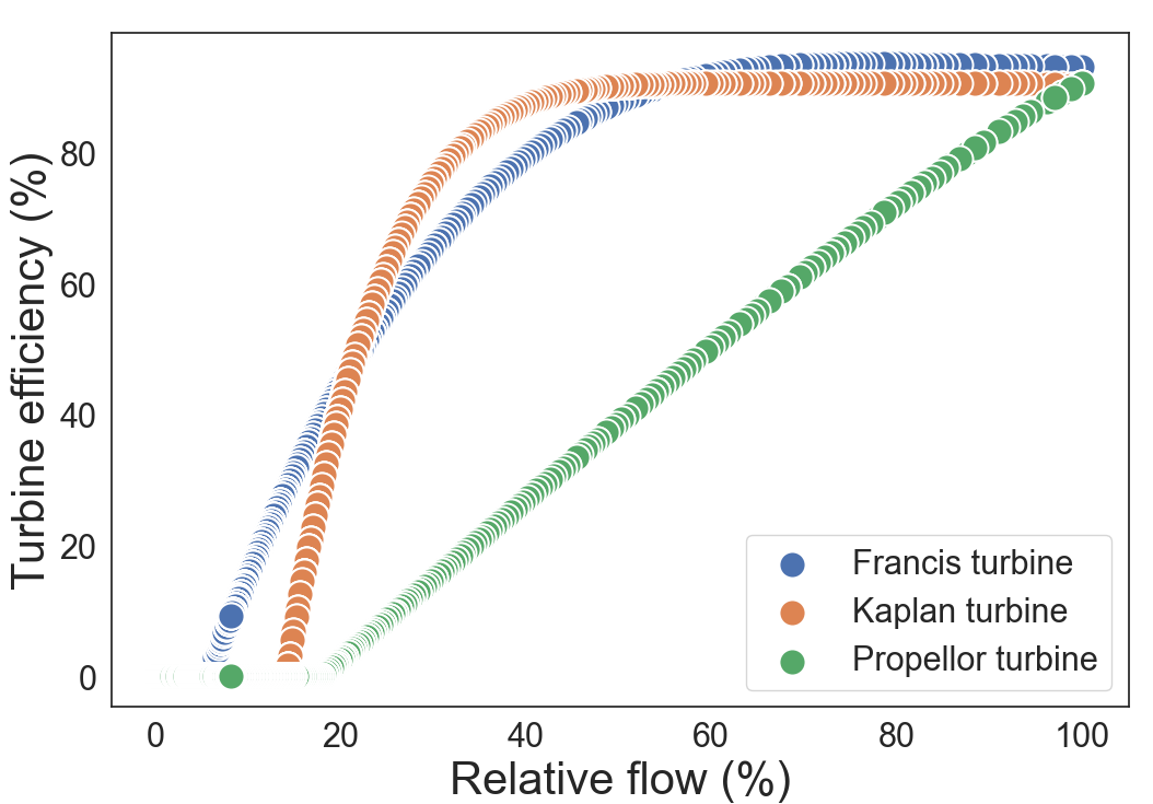
Figure 1: Efficiency curves for different turbines using HydroGenerate.

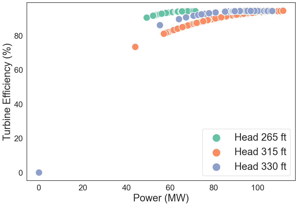
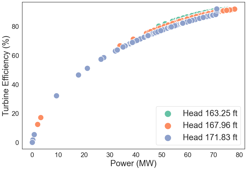
Figure 2: Operational efficiency of a Francis turbine for two plants located in western USA has been shown (a) Plant A with three operating heads 265 ft., 315 ft. and 330 ft. and (b) Plant B with three operating heads 163.25 ft., 167.96 ft. and 171.83 ft.

By utilizing data from two different plants located in western continental USA we calculate the efficiency parameters from two plants as shown in Fig. 2(a) and (b).

IV Interdependency Evaluation

Several factors are a contributing factor upon how hydropower plants located in different watersheds respond. Internal response is affected by the operation of the storage reservoirs upstream by controlling the volume of water stored or released. There are several external factors like minimum water limits, fish habitats, recreation etc. that restrict its operation. The water management authorities responsible for maintaining water regulation, these are a mix of complex rules, policies and agreements that are regulated by Federal laws. There are three major watersheds in continental USA- the Columbia river, the Colorado river and the Tennessee river.

Columbia river basin has its largest foothold in the Pacific Northwest Region having 250 reservoirs and 150 hydroelectric projects [13]. Streamflow in the Columbia river watershed does not follow the electricity demand, where the peak is mostly observed during the winter months however the flow peaks in spring and early summer when the snow pack melts. Although recent changes in climate conditions have made some of those patterns erratic. The high rate of correlation between their power generation can be utilized to understand the operating range for patterns in the plants located in the Columbia basin. The variation is not limited by flow but is a function of season and head as well.

IV-A Methodology

Considering water time constant and distance between the two plants it is essential to establish a time correlation between the streamflow data. Data was split into three prominent seasons Winter, Spring and Summer. As discussed before streamflow does depend on the season and thus the time lag for each season needs to be evaluated to establish a comprehensive understanding. Upon analysis the time correlation for the three seasons were seen to peak the highest between 1hr and 2hr, a representative plot for Winter is shown in Fig. 3.

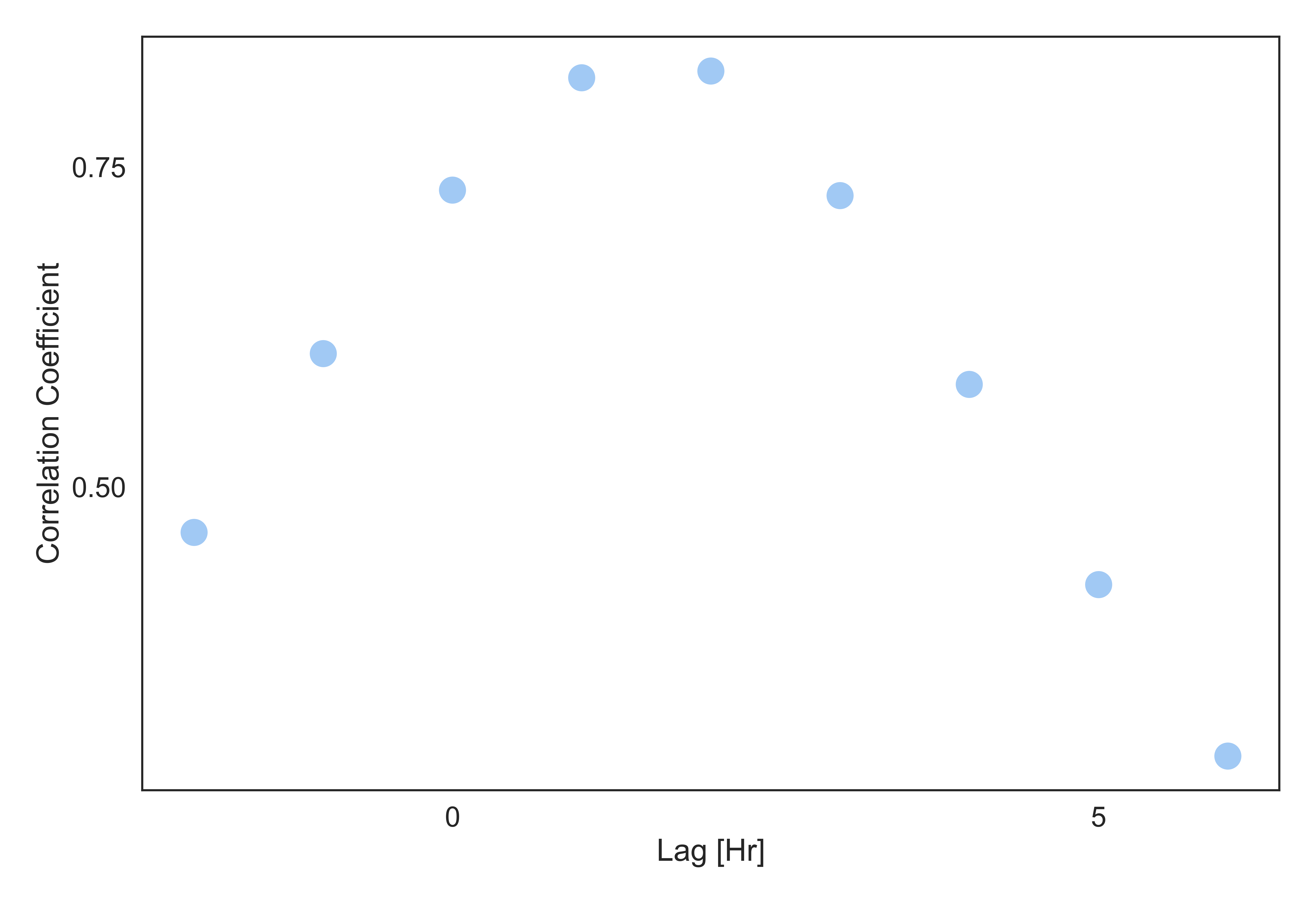
Figure 3: Time correlation of streamflow between Plant A and B during Winter.

Using this information the original dataset was re-organised to match the time delay to establish a relationship between their power dispatch. For the analysis we further added incorporated the head parameter of the upstream plant that influences the power generation downstream.

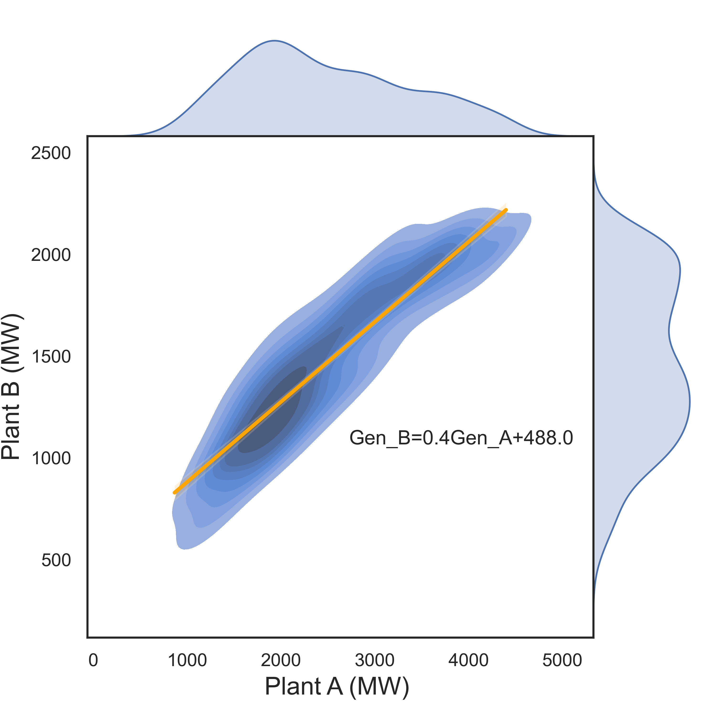
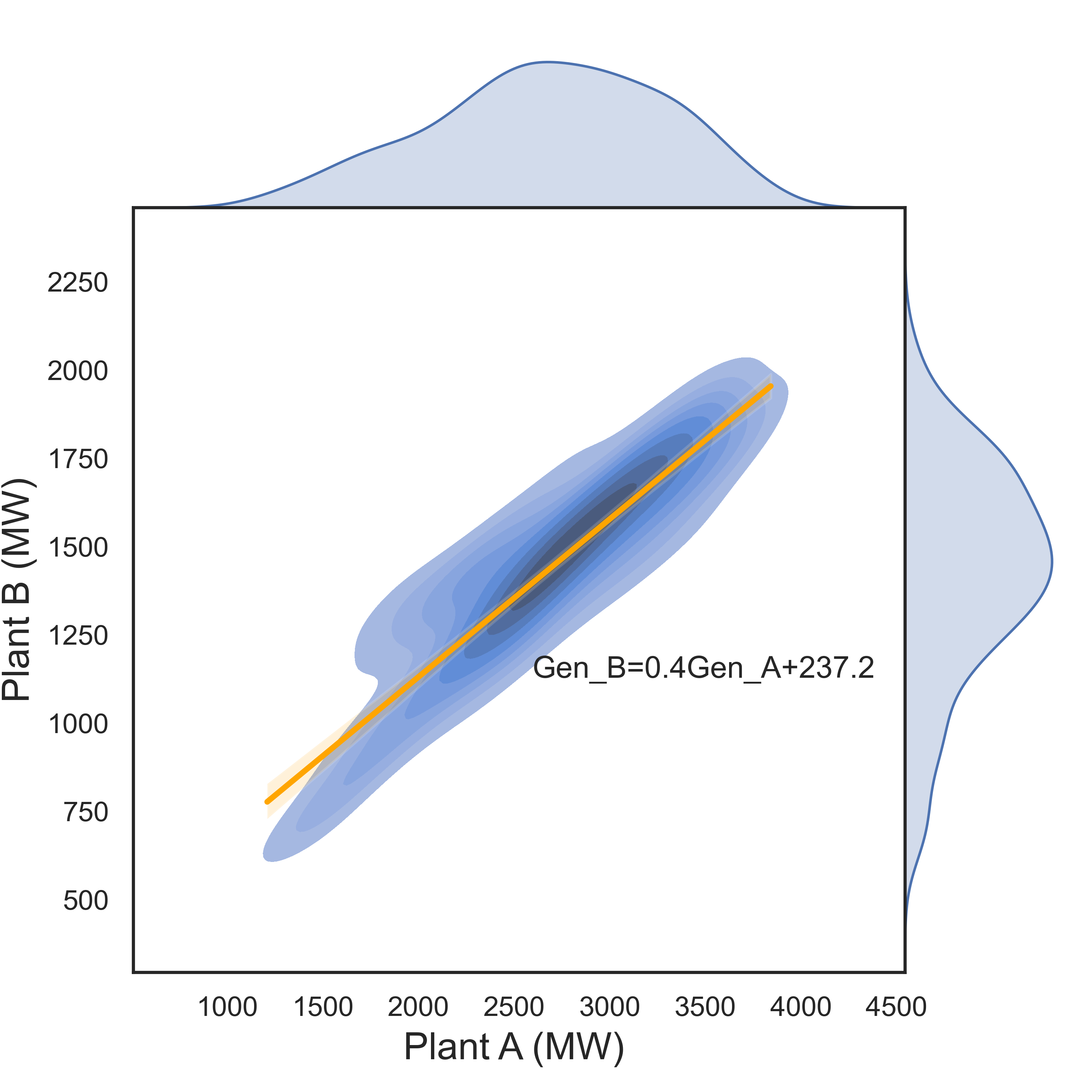
Figure 4: Generation comparison for Winter (a) Head for upstream plant (Plant A) is $294.34ft.$, (b) Head for upstream plant (Plant A) is $322.45ft.$

As it can be seen in Fig. 4 that within the same season the generation for the two plants A and B show a significant variation with the change in head. A similar significance can be seen for the Summer season when variation of head is considered. A relationship between the generation patterns of the rivers upstream and downstream were obtained using linear regression of the power dispatch.

IV-B Unit-Level Dispatch using Regression Models

With plant-level time series recordings and unit-level measurements, one can build regression models to correlate water head, total power output, etc., with individual generator’s status and power output. In this study, machine learning, more specifically Deep Neural Networks (DNN), is implemented to build regression models in view of its rapid development and wide applications in many engineering problems. Previous studies [14] have proven the high precision of DNN-based regression models and the impressive advantages over the conventional regression model construction approaches. A 6-layers fully connected DNN has been utilized for this approach.

For upstream plant A mentioned above, there are a total of 5089 recordings at each hour in three seasons. Each recording comprises plant-level and unit-level data: Plant-level data contains total power output, water head, water storage, generator flow rate, spillage, etc. Power output, water head and water storage were selected as model input parameters. Unit-level data contain the status and power outputs of 30 generators. These generator units can be classified into 4 categories C1, C2, C3 and C4, according to the nominal power. Status and power outputs of individual generators can be converted into a number of active units and power output of 4 categories, as shown in Fig. 5.

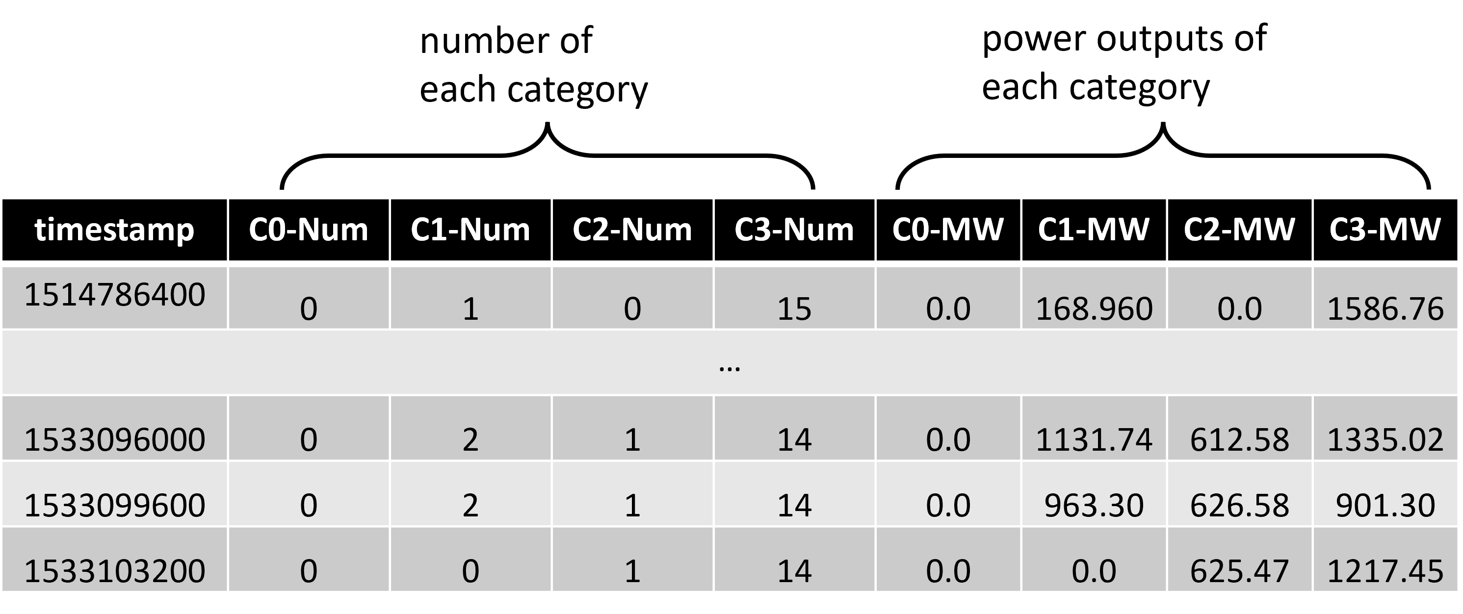
Figure 5: Unit-level data as model outputs.

IV-B1 Training

Fig. 6 shows the 2-step model training procedure. As can be seen in the right plots, the number of active units and the power output of Category ”C1” were re-organized as three columns: ”C1-Exist” indicates if there is an active unit in this category, ”C1-MW” is the total power of this category and ”C1-unitMW” is the average power output of each active unit in this category. In Step 1, a DNN-based classifier is trained to correlate model inputs with ”C1-Exist”; In Step 2, a DNN-based regression model is developed between model inputs and ”C1-MW”, ”C1-unitMW” for ”active” data only (data in red dotted line). For the models in Fig. 6, the DNN-based classifier can predict whether Category ”C1” has active units with an accuracy of 91.45%. The 80% confidence intervals of the regression model are smaller than 10% of the mean values.

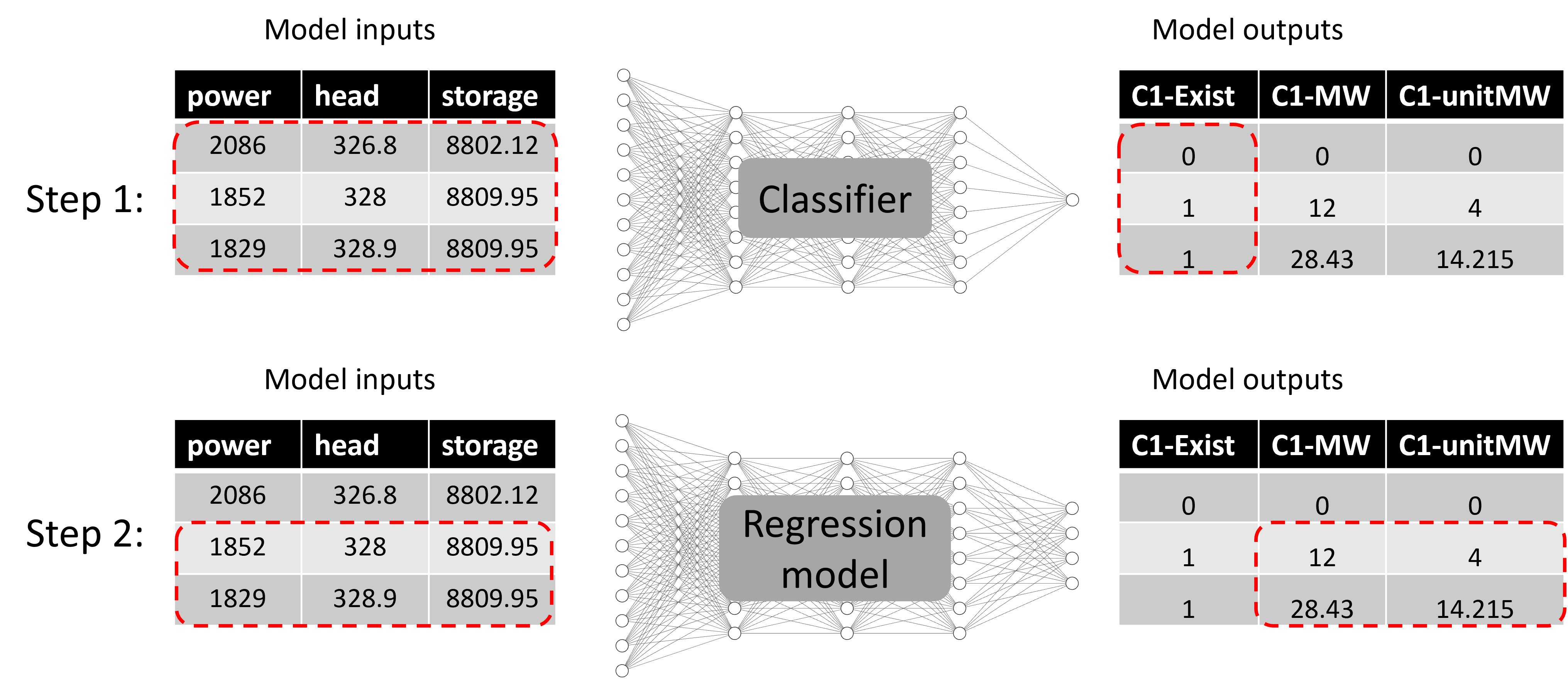
Figure 6: Model training procedure.

IV-B2 Testing and Results

By repeating the above procedure, one can obtain regression models for all categories. With these trained models, one can predict unit-level conditions from an appropriate combination of plant-level parameters. An example is given in Fig. 7. Later, by allocating the total power output to the active units in each category, unit-level dispatch can be conducted according to the plant-level inputs.

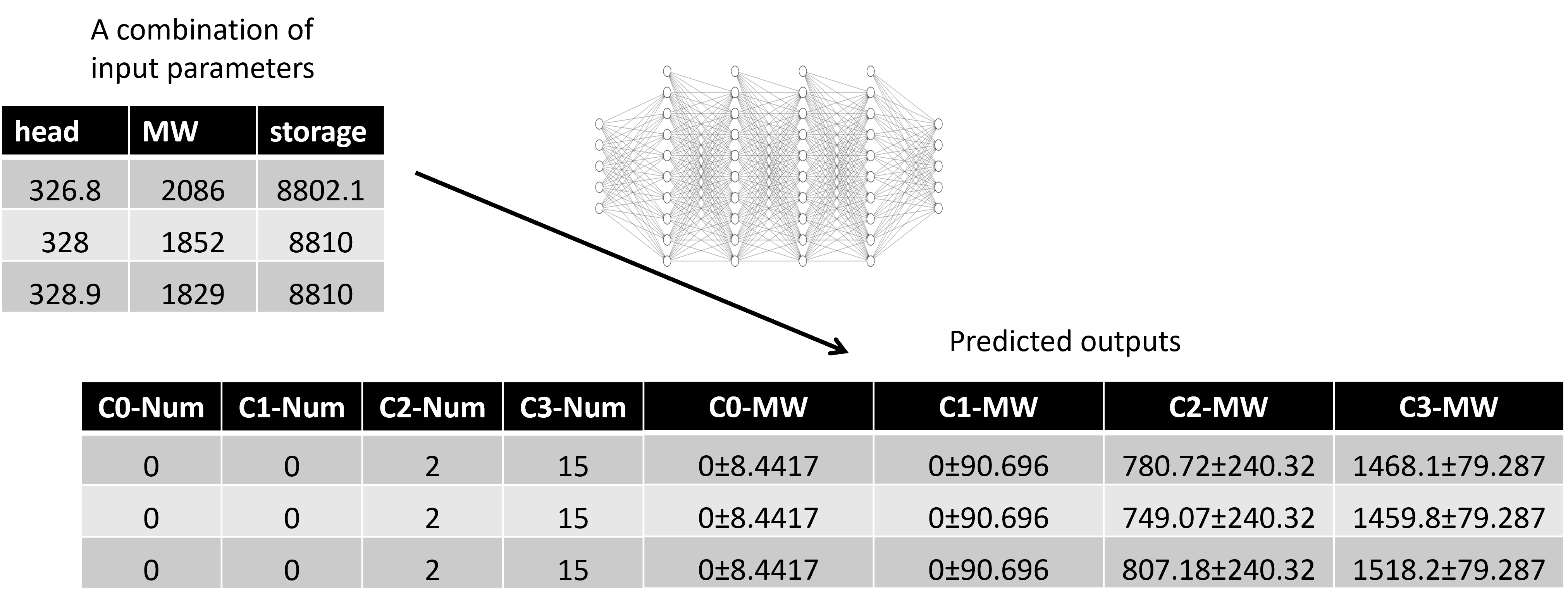
Figure 7: An example of model prediction for plant A.

IV-C Integration and GUI development

To integrate the individual tools and algorithms described above, a GUI is developed for the Hy-DAT tool as an interface for the hydropower database and the suite of tools as illustrated in Fig. 8.

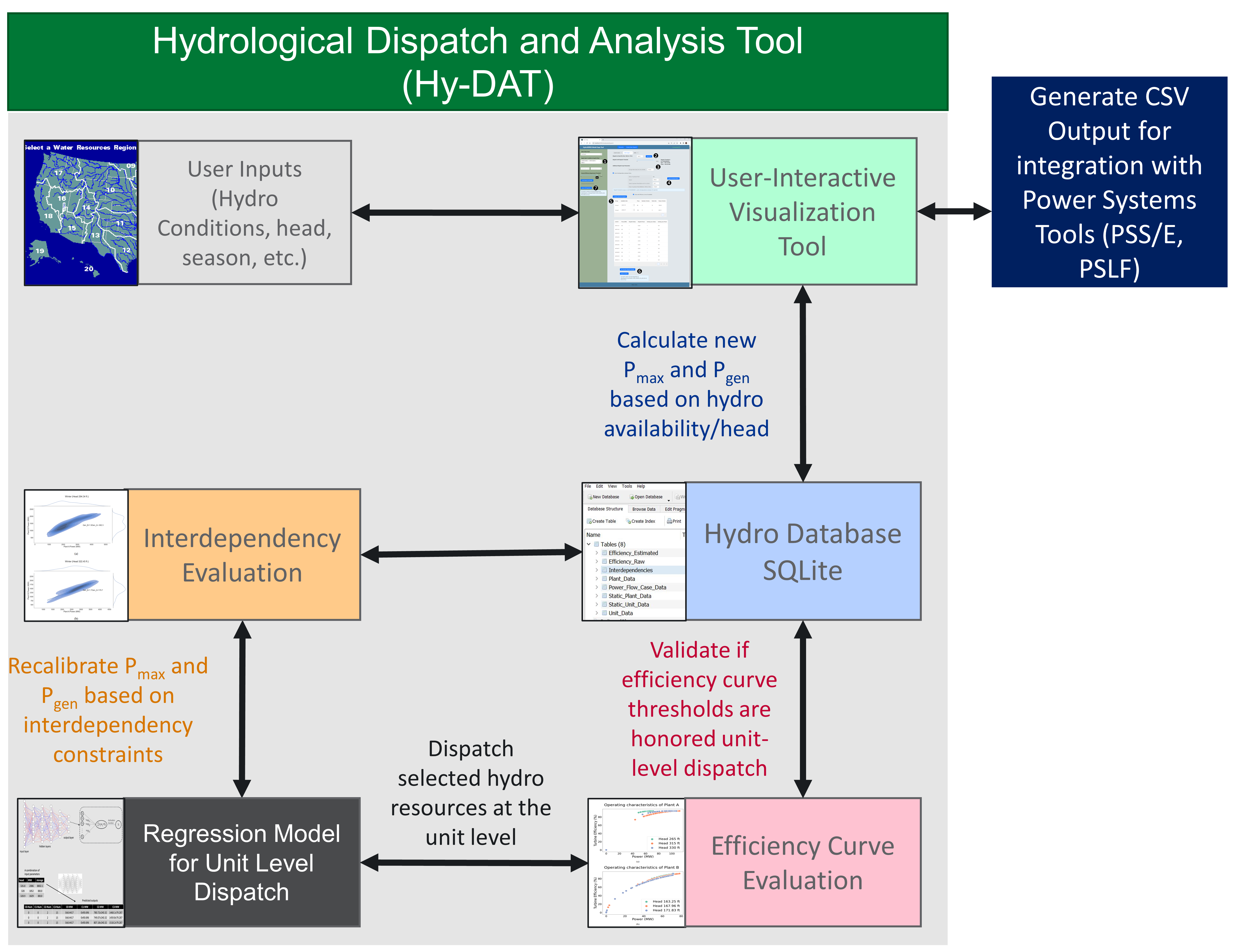
Figure 8: Integration using GUI

TABLE III: Unit-level dispatch results

Project	Unit ID	$P_{gen}$ (MW)	$P_{max}$ (MW)	Head (ft.)	$P_{gen}$ calculated (MW)	$P_{max}$ available (MW)
Plant A	1	600	707	307.1	361	513.65
Plant A	1	650	707	307.1	361	513.65
Plant A	1	650	707	307.1	361	513.65
Plant A	1	614.2	825.7	307.1	0	599.88
Plant A	1	700	825.7	307.1	553.97	599.88
Plant A	1	700	825.7	307.1	553.97	599.88
Plant A	1	105	125	307.1	79.48	90.81
Plant A	2	105	125	307.1	79.48	90.81
Plant A	3	105	125	307.1	79.48	90.81

The GUI allows users to select specific or all hydropower plants and specify a hydro-condition either using a historical timeframe or by providing specific hydropower conditions like dry/wet/average water year, and season of operation. Based on the user inputs, a visualization is also available to plot and evaluate the various hydrological parameters for historical years. Based on the user inputs, the tool calculates the MW target and available capacity for the selected hydropower resources. However, due to inter-dependency constraints, some plants in downstream especially the run-of-river plants have to re-calibrate the MW target based on the water availability and release from the plants/dams upstream. The re-calibrated MW targets are passed on the unit-level dispatch tool which uses trained AI regression models based on the historical database to dispatch the selected resources based on the available head, water availability, and MW target for the plant. Finally, the unit-level dispatches are validated using pre-calculated efficiency curves datasets from the database to make sure units are dispatched above the efficiency threshold else the unit dispatches are corrected. Finally, the updated MW target and hydropower operational characteristics are available to be exported for planning and operational studies, as shown in Table III. For each generator, it contains unit information, power output from an existing power flow case for reference, and dispatch power output.

V Concluding Remarks

Operation and planning reliability studies currently do not consider environmental conditions and constraints such as water availability and interdependencies among power plants. The reason for such an approach is lack of coupling of hydro conditions and constraint with the electrical model used in power system planning and operation studies (power flow and dynamic models). Industry develops base cases for heavy winter and summer loading conditions as well as shoulder cases representing light loading conditions. In the environment of large renewable penetration of intermittent resources (solar and wind) and carbon-free goals, hydro becomes a more critical resource. For this reason, it is important to properly represent hydro conditions in base cases and, similar to developing cases having heavy and light load conditions, we need to have high and low hydro conditions properly represented in steady-state and dynamic models used for power system planning and operation reliability studies. This paper provides an end-to-end methodology for addressing modeling gaps in hydropower resources using a newly tool Hy-DAT that incorporates use of a developed database and set of tools and algorithms to use historical data in accurately dispatching hydropower resources.

References

[1]
B. Mitra, S. Datta, S. Kincic, N. Samaan, and A. Somani, “Gaps in
representations of hydropower generation in steady-state and dynamic
models,” in 2024 ISGT NA, 2024.
[2]
S. Kincic, N. Samaan, S. Datta, A. Somani, H. Yuan, J. Tan, R. Bhattarai, and
T. M. Mosier, “Hydropower modeling gaps in planning and operational
studies,” 11 2022.
[3]
D. Kosterev, “Hydro turbine-governor model validation in pacific northwest,”
IEEE Transactions on Power Systems, vol. 19, no. 2, 2004.
[7]
C. Powertech Labs Inc. Surrey, British Columbia, “Transient security
assessment tool user manual,” 2011.
[8]
U. B. H. Association, “Us army corps of engineers.”
[9]
E. S. H. Association, “Guide on how to develop a small hydropower plant,”
2004.
[10]
B. A. Bhatti, S. Hanif, J. Alam, B. Mitra, R. Kini, and D. Wu, “Using energy
storage systems to extend the life of hydropower plants,” Applied
Energy, vol. 337, p. 120894, 2023. [Online]. Available:
https://www.sciencedirect.com/science/article/pii/S0306261923002581
[11]
B. Mitra, J. F. Gallego-Calderon, S. N. Elliott, T. M. Mosier, U. O.
of Energy Efficiency, and R. Energy, “Hydrogenerate: Open source python tool
to estimate hydropower generation time-series, version 3.6 or newer,” 10
2021.
[12]
B. Mitra, S. Elliott, J. Koudelka, C. Davis, T. Mosier, D. Anderson, and
J. Saulsbury, “Development and role of microgrids surrounding modernized
irrigation district,” in AGU Fall Meeting Abstracts, vol. 2020, 2020,
pp. SY051–03. [Online]. Available:
https://irrigationviz.pnnl.gov/docs/modules/hydropower
[14]
D. Wang, J. Bao, Z. Xu, B. Koeppel, O. A. Marina, A. Noring,
M. Zamarripa-Perez, A. Iyengar, E. Eggleton, D. T. Schwartz et al.,
“Machine learning tools set for natural gas fuel cell system design,”
ECS Transactions, vol. 103, no. 1, p. 2283, 2021.