Communication Efficient ConFederated Learning: An Event-Triggered SAGA Approach

Abstract

Federated learning (FL) is a machine learning paradigm that targets model training without gathering the local data dispersed over various data sources. Standard FL, which employs a single server, can only support a limited number of users, leading to degraded learning capability. In this work, we consider a multi-server FL framework, referred to as Confederated Learning (CFL), in order to accommodate a larger number of users. A CFL system is composed of multiple networked edge servers, with each server connected to an individual set of users. Decentralized collaboration among servers is leveraged to harness all users’ data for model training. Due to the potentially massive number of users involved, it is crucial to reduce the communication overhead of the CFL system. We propose a stochastic gradient method for distributed learning in the CFL framework. The proposed method incorporates a conditionally-triggered user selection (CTUS) mechanism as the central component to effectively reduce communication overhead. Relying on a delicately designed triggering condition, the CTUS mechanism allows each server to select only a small number of users to upload their gradients, without significantly jeopardizing the convergence performance of the algorithm. Our theoretical analysis reveals that the proposed algorithm enjoys a linear convergence rate. Simulation results show that it achieves substantial improvement over state-of-the-art algorithms in terms of communication efficiency.

I Introduction

The tremendous advancement of machine learning (ML) has rendered it a driving force for various research fields and industrial applications. However, the traditional ML framework follows a centralized fashion which assembles the training data to a central computing unit (CPU) where model training is performed. Such an approach might be problematic when data is confidential or when transferring the training data to the CPU is unrealistic. With a growing interest in data privacy, regulations like GDPR (General Data Protection Regulation) and ADPPA (American Data Privacy and Protection Act) have imposed restrictions on sharing privacy-sensitive data among different clients or platforms. As such, breaking the data-privacy barrier is an urgent and meaningful task.

Federated Learning (FL) [1, 2] is an emerging machine learning paradigm that enables model training without transferring local data to the CPU. FL has drawn significant attention from both academia and industry, especially for privacy-sensitive and data-intensive applications. A standard FL system consists of a server and a set of devices/users. In general, FL addresses privacy protection by adopting a compute-then-aggregate (CTA) approach. More precisely, in each iteration the server first broadcasts the global model vector to the users. Each user then computes a local gradient using its own data, and uploads its local gradient to the server. At the end of each iteration, the server performs one step of gradient descent (using the aggregated gradient) to obtain an updated global model vector. This process cycles until model training is accomplished. Typically, the training process takes a large number of iterations to converge. Thus FL may consume a substantial amount of communication resources. Therefore, it is important to reduce the communication overhead to an affordable level. To this end, various methods were developed along different research lines, including methods which aim at improving the convergence speed [3, 4, 5, 6, 7, 8, 9, 10, 11, 12, 13, 14, 15], methods that reduce the amount of transmission by selecting only a subset of users for uploading their gradients [16, 17, 18, 19, 20, 21, 22, 23, 24], methods that sparsify or quantize the local gradients [25, 26, 27, 28, 29, 30, 31, 32, 33, 34], or combinations of these techniques.

Besides the excessively high communication cost, another restriction of FL is that conventional FL systems employ only a single server. Due to the limited communication capacity, the number of users that can be served by a single server is limited. To involve more devices for model training, an alternative framework to the standard single-server FL is a decentralized FL system [35, 36, 37, 38, 39, 15, 40, 41, 42, 43]. A decentralized FL system is composed of a number of nodes or agents which are able to perform computation and communication. Each node carries its own training data. Different nodes form a decentralized network in which only neighboring nodes can either bidirectionally or directionally [44, 45, 46] communicate with each other. In decentralized FL, the training process follows a similar CTA mode as in the standard system, except that the local gradient or local model vector is exchanged among neighboring nodes. Despite its scalability, decentralized FL is confined to D2D (device-to-device) type networks which requires D2D communications that may not be easily achieved in cellular systems.

Recently, a new FL framework termed Confederated Learning (CFL) was proposed in [47] to overcome the drawbacks of existing FL systems. A CFL system consists of multiple servers, in which each server is connected with an individual set of users as in the conventional FL framework. Decentralized collaboration among servers is leveraged to make full use of the data dispersed over different users. CFL can be considered as a hybrid of standard and decentralized FL systems. In particular, CFL degenerates to standard FL when there is only a single server. Although there exist a plethora of algorithms/convergence analyses for standard FL, the extension of these results to CFL is not straightforward since the latter framework involves decentralized collaboration among servers. On the other hand, CFL becomes a decentralized FL system when there is no user, namely, when each server itself carries the training data. In this case, each server’s data are readily accessible to this server without any communication cost. This is in sharp contrast to the CFL framework whose communication cost mainly comes from collecting training information by each server from its associated users. Therefore, existing gradient tracking-based decentralized optimization methods [40, 41, 44, 45, 46], when applied to CFL, lead to an unsatisfactory communication efficiency. In [47], a stochastic ADMM algorithm with random user selection is developed for CFL. However, the ADMM-based method is proved to possess only a sub-linear convergence rate, and its performance relies heavily on man-crafted parameters that can be hard to tune in real-world applications.

In this paper, we propose a gradient-based method for communication-efficient CFL. The proposed algorithm is based on the framework of GT-SAGA (gradient tracking with stochastic average gradient) [40]. To reduce the amount of data transmission between servers and users, a conditionally-triggered user selection (CTUS) mechanism is developed. CTUS sets a computationally verifiable selection criterion at the user side such that only those users whose VR-SGs (variance-reduced stochastic gradients) are sufficiently informative report their VR-SGs to their associated servers. At the server side, the aggregated gradient is obtained by integrating the uploaded VR-SGs as well as the stale VR-SGs corresponding to those unreported users. The CTUS mechanism shares a similar spirit with the even-triggering-based methods proposed for standard FL or traditional decentralized optimization methods [48, 49, 43, 50, 51, 52, 34, 22, 23, 53, 24]. Nevertheless, the selection criterion developed in this paper is very different from existing methods. Specifically, for multi-server systems, the variables from neighboring servers should be taken into account in the design of the selection criterion. Simulation results show that the proposed CTUS mechanism helps preclude most of those non-informative user uploads, thereby striking a higher communication efficiency than state-of-the-art algorithms.

The rest of this paper is organized as follows. In Section II, we introduce the confederated learning problem along with some assumptions on the objective function as well as the server network. Then, in Section III, we provide a brief overview of the classic gradient tracking (GT) method as well as the GT-SAGA method that can be adapted to solve the CFL problem. The proposed method is presented in Section IV, with the convergence analysis given in Section V. The proof of the main theoretical result, namely, Theorem 1, is provided in Section VI. In section VII, we also provide theoretical analysis to justify that the proposed CTUS can save user uploads under mild conditions. Simulations results are presented in Section VIII, followed by concluding remarks in Section IX.

II Problem Formulation

II-A CFL Framework

We consider a confederated learning (CFL) framework consisting of $N$ networked edge servers. Figure 1 depicts a schematic of CFL. The connective relation of these edge servers is described by an undirected connected graph $G=\{V,E\}$, where $V$ (resp. $E$) denotes the set of servers (resp. edges). The $i$th edge server serves $P_{i}$ users. Each user is only allowed to communicate with its associated server. In addition to communicating with its own users, each server can communicate with its neighboring servers. With the confederated network, we aim to solve the following CFL problem:

$$\mathop{\min}\limits_{\boldsymbol{x}\in\mathbb{R}^{d}} \ \textstyle f(\boldsymbol{x})\triangleq\frac{1}{N}\sum_{i=1}^{N}f_{i}(\boldsymbol{x}),$$ (1)

where $\boldsymbol{x}\in\mathbb{R}^{d}$ is the model vector to be learned, $f_{i}(\boldsymbol{x})=\sum_{j=1}^{P_{i}}f_{ij}(\boldsymbol{x})$, $f_{ij}(\boldsymbol{x})=\sum_{t=1}^{S_{ij}}f_{ij,t}(\boldsymbol{x})$ is the loss function held by user $u_{ij}$, $f_{ij,t}(\boldsymbol{x})$ is the loss function corresponding to the $t$th training sample at user $u_{ij}$, and $S_{ij}$ is the number of training samples at user $u_{ij}$. Here user $u_{ij}$ refers to the $j$th user served by the $i$th server. It is also noteworthy that $f_{ij,t}$ may corresponds to a mini-batch of training samples instead of a single sample.

The communication bottleneck of CFL lies in the user-to-server (U2S) communications. Existing methods are designed either for standard single-server FL or for decentralized FL. Standard FL methods cannot be straightforwardly extended to the CFL, while decentralized FL methods neglect the U2S communications in their algorithmic development. Focusing on problem (1), we aim to develop a communication-efficient method which seeks to reduce the U2S communication overhead.

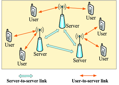
Figure 1: The CFL framework with multiple servers.

II-B Function and Server-Network Assumptions

We assume that $f$ (resp. $\nabla f$) is $\mu$-strongly convex (resp. $L$-Lipschitz continuous) while both $f$, $f_{i}$, $f_{ij}$ and $f_{ij,t}$ are continuously differentiable with their gradients being $L$-Lipschitz continuous. The definitions of $\mu$-strongly convexity and $L$-Lipschitz continuity are given below.

Definition 1.

(Strongly convexity) A function $f:\mathbb{R}^{d}\rightarrow\mathbb{R}\cup\{+\infty\}$ is said to be $\mu$-strongly convex if

$$\textstyle f(\boldsymbol{y})\geq f(\boldsymbol{x})+\langle\nabla f(\boldsymbol{x}),\boldsymbol{y}-\boldsymbol{x}\rangle+\frac{\mu}{2}\|\boldsymbol{y}-\boldsymbol{x}\|_{2}^{2},\ \forall\boldsymbol{x},\boldsymbol{y}.$$ (2)

Definition 2.

(Lipschitz continuity) The gradient of $f:\mathbb{R}^{d}\rightarrow\mathbb{R}\cup\{+\infty\}$ is said to be $L$-Lipschitz continuous if

$$\|\nabla f(\boldsymbol{x})-\nabla f(\boldsymbol{y})\|_{2}\leq L\|\boldsymbol{x}-\boldsymbol{y}\|_{2},\ \forall\boldsymbol{x},\boldsymbol{y}.$$ (3)

Recall that the servers form a bidirectionally connected graph $G=\{V,E\}$. Denote $\boldsymbol{W}\in\mathbb{R}_{+}^{N\times N}$ as the mixing matrix associated with the graph $G$. It is assumed that $\boldsymbol{W}$ is symmetric, primitive and doubly stochastic. In particular, $w_{ii^{\prime}}$ which is the $(i,i^{\prime})$th element of $\boldsymbol{W}$ equals to $0$ (resp. nonzero) if server $i$ and $i^{\prime}$ are unconnected (resp. connected). For such a $\boldsymbol{W}$, its largest singular value is $1$ (with multiplicity equals to $1$), with its corresponding singular vector being $\frac{1}{\sqrt{N}}\boldsymbol{1}_{N}$. The second largest singular value of $\boldsymbol{W}$, denoted as $\sigma$, is thus equal to $\|\boldsymbol{W}-\frac{1}{N}\boldsymbol{1}_{N}\boldsymbol{1}_{N}^{T}\|_{2}$ and is smaller than $1$. Notably, $\boldsymbol{W}$ can be conveniently obtained as $\boldsymbol{W}=\boldsymbol{I}-\frac{\boldsymbol{L}}{\tau}$, where $\boldsymbol{L}$ is the Laplacian matrix of $G$ and $\tau>\frac{1}{2}\lambda_{\text{max}}(\boldsymbol{L})$ is a scaling factor.

III Overview of GT and GT-SAGA

Our proposed algorithm is based on the gradient tracking (GT) framework [54]. In this section, we begin with a brief introduction of GT and then introduce the GT-SAGA algorithm [40] which is a practical variant of GT. GT-SAGA is designed for solving decentralized optimization problems. We will discuss how to adapt GT-SAGA to solve the CFL problem (1) in Section III-C.

III-A Gradient Tracking

GT [54] is designed for solving decentralized optimization problems of the following form:

$$\textstyle\mathop{\min}\limits_{\boldsymbol{x}\in\mathbb{R}^{d}}\ F(\boldsymbol{x})\triangleq\frac{1}{N}\sum_{i=1}^{N}f_{i}(\boldsymbol{x}),$$ (4)

where $f_{i}(\boldsymbol{x})=\sum_{t=1}^{P_{i}}f_{i,t}(\boldsymbol{x};\mathcal{D}_{i,t})$ is the local loss function held by node $i$ and $f_{i,t}(\boldsymbol{x})$ is the loss function associated with the $t$th training samples stored at node $i$. GT is usually compactly written as

$$\text{GT}:\ \textstyle\boldsymbol{x}_{i}^{k+1}=\sum_{i^{\prime}=1}^{N}w_{ii^{\prime}}\boldsymbol{x}_{i^{\prime}}^{k}-\alpha\boldsymbol{y}_{i}^{k},\ 1\leq i\leq N,$$ (5)

$$\textstyle\boldsymbol{y}_{i}^{k+1}=\sum_{i^{\prime}=1}^{N}w_{ii^{\prime}}\boldsymbol{y}_{i^{\prime}}^{k}+\nabla f_{i}(\boldsymbol{x}_{i}^{k+1})-\nabla f_{i}(\boldsymbol{x}_{i}^{k}),\ 1\leq i\leq N.$$ (6)

Note that GT is designed for a D2D network in which each node carries its own training data and each node can communicate with its neighboring nodes. In GT, each node holds two variables, $\boldsymbol{x}_{i}$ and $\boldsymbol{y}_{i}$. After the $(k+1)$th iteration, each node exchanges $(\boldsymbol{x}_{i}^{k+1},\boldsymbol{y}_{i}^{k+1})$ with its neighboring nodes. The core idea behind GT is the combination of decentralized gradient descent (DGD) and dynamic average consensus (DAC). To see this, omitting the DAC step, i.e., (6), and assuming that $\boldsymbol{y}_{i}^{k}=\nabla f_{i}(\boldsymbol{x}_{i}^{k})$, then GT degenerates to the standard DGD algorithm, in which $\alpha$ is the stepsize. However, it is well known that the exact convergence of DGD can not be guaranteed unless a decreasing stepsize is employed. The problem is that a decreasing stepsize can only offer a sublinear convergence rate even if $f_{i}$ is strongly convex. In GT, the DAC mechanism is incorporated to remedy this drawback of DGD. DAC is an efficient tool to track the average of time-varying signals. Formally, suppose each node $i$ measures a time-varying signal $r_{i}^{k}$ at time $k$ and consider the problem of tracking its average $\bar{r}^{k}=\frac{1}{N}\sum_{i=1}^{N}r_{i}^{k}$ at each node. The DAC mechanism, which is mathematically stated as

$$\textstyle d_{i}^{k+1}=\sum_{i^{\prime}=1}^{N}w_{ii^{\prime}}d_{i^{\prime}}^{k}+r_{i}^{k+1}-r_{i}^{k},\ \forall i,$$ (7)

converges to $\bar{r}^{k+1}$ provided that $\lim_{k\rightarrow\infty}|r_{i}^{k+1}-r_{i}^{k}|=0$. In GT, we intend to track the average of the local gradients $\frac{1}{N}\sum_{i=1}^{N}\nabla f_{i}(\boldsymbol{x}_{i}^{k})$ instead of using only the local gradient $\nabla f_{i}(\boldsymbol{x}_{i}^{k})$ at every node. This generates the DAC step (6). If the local variables tend to arrive at a consensus state, i.e. $\boldsymbol{x}_{i}^{k}\rightarrow\boldsymbol{x}$, which also means that $\nabla f_{i}(\boldsymbol{x}_{i}^{k+1})-\nabla f_{i}(\boldsymbol{x}_{i}^{k})\rightarrow 0$, then (6) ensures that $\boldsymbol{y}_{i}^{k}\rightarrow\frac{1}{N}\sum_{i=1}^{N}\nabla f_{i}(\boldsymbol{x})$ and thus (5) degenerates to a gradient descent step applied to the whole objective function $F$. As such, GT is guaranteed to converge to the global optimum with a linear convergence rate, under the strongly convexity assumption.

III-B Gradient Tracking with Variance Reduction

In machine learning applications, each user may hold a large number of training samples and thus it is neither practical nor efficient to compute the full local gradient $\nabla f_{i}(\boldsymbol{x}_{i}^{k+1})$. An alternative solution is to compute a stochastic approximation of $\nabla f_{i}(\boldsymbol{x}_{i}^{k+1})$. However, directly employing the stochastic gradient introduces a non-vanishing variance and would consequently undermine the exact convergence of GT. To alleviate this problem, GT-SAGA [40], summarized in Algorithm 1, was proposed to incorporate a variance-reduced stochastic gradient (VR-SG) $\boldsymbol{g}_{i}^{k+1}$ to replace $\nabla f_{i}(\boldsymbol{x}_{i}^{k+1})$. The VR-SG is an unbiased estimate of $\nabla f_{i}(\boldsymbol{x}_{i}^{k+1})$ in the sense that $\mathbb{E}_{t_{i}^{k+1}}\{\boldsymbol{g}_{i}^{k+1}\}=\nabla f_{i}(\boldsymbol{x}_{i}^{k+1})$. More importantly, the variance of $\boldsymbol{g}_{i}^{k+1}$ which is mathematically stated as $\mathbb{E}_{t_{i}^{k+1}}\{\|\boldsymbol{g}_{i}^{k+1}-\nabla f_{i}(\boldsymbol{x}_{i}^{k+1})\|_{2}^{2}\}$ tends to $0$ if the algorithm converges. Thanks to the VR technique, GT-SAGA is guaranteed to converge to the global optimum while still maintaining a linear convergence rate.

In addition to GT-SAGA, there also exist other variance reduction-based gradient tracking methods, e.g. [40, 41, 44, 45, 46]. Among them, Push-SAGA/AB-SAGA [44, 45] and Push-SVRG/AB-SVRG [46] are designed for directed networks, GT-SVRG [40] and GT-SARAH [41] are based on double-loop variance reduction techniques that periodically demand all users to upload their local gradients to their respective servers. Such a requirement poses practical challenges in the FL setting.

Algorithm 1 GT-SAGA

  Input: $N$, $\{P_{i}\}$, $\boldsymbol{W}$, $\alpha$, $\{\boldsymbol{x}_{i}^{0},\boldsymbol{y}_{i}^{0},\boldsymbol{\phi}_{i,t}^{0}=\boldsymbol{0}\}_{i=1,t=1}^{i=N,t=P_{i}}$.

  while not converge do

   For each node parallel do

     1. Node $i$ computes $\boldsymbol{x}_{i}^{k+1}=\sum_{i^{\prime}=1}^{N}w_{ii^{\prime}}\boldsymbol{x}_{i^{\prime}}^{k}-\alpha\boldsymbol{y}_{i}^{k}$;

     2. Node $i$ uniformly generates a random integer $t_{i}^{k+1}$, $1\leq t_{i}^{k+1}\leq P_{i}$, and then computes the VR-SG via

$$\textstyle\boldsymbol{g}_{i}^{k+1}= P_{i}\cdot(\nabla f_{i,t_{i}^{k+1}}(\boldsymbol{x}_{i}^{k+1})-\nabla f_{i,t_{i}^{k+1}}(\boldsymbol{\phi}_{i,t_{i}^{k+1}}^{k}))+$$

$$\textstyle\sum_{t=1}^{P_{i}}\nabla f_{i,t}(\boldsymbol{\phi}_{i,t}^{k}),$$ (8)

Set $\nabla f_{i,t_{i}^{k+1}}(\boldsymbol{\phi}_{i,t_{i}^{k+1}}^{k+1})=\nabla f_{i,t_{i}^{k+1}}(\boldsymbol{x}_{i}^{k+1})$ and also set $\nabla f_{i,t}(\boldsymbol{\phi}_{i,t}^{k+1})=\nabla f_{i,t}(\boldsymbol{\phi}_{i,t}^{k})$, $\forall t\neq t_{i}^{k+1}$;

     3. Node $i$ computes $\boldsymbol{y}_{i}^{k+1}=\sum_{i^{\prime}=1}^{N}w_{ii^{\prime}}\boldsymbol{y}_{i^{\prime}}^{k}+\boldsymbol{g}_{i}^{k+1}-\boldsymbol{g}_{i}^{k}$ and then broadcasts ($\boldsymbol{x}_{i}^{k+1}$,$\boldsymbol{y}_{i}^{k+1}$) to its neighboring nodes;

   End For End while and Output $\boldsymbol{x}^{k+1}$;

III-C Adapting GT-SAGA for CFL

Now we discuss how to modify GT-SAGA to make it applicable for solving (1). Adjusting GT-SAGA to solve (1) can be realized by treating node $i$ in Algorithm 1 as server $i$. In the CFL setting, despite the fact that the training data are stored at users, we can randomly select a user and let the user randomly pick a mini-batch set of training samples to compute the local gradient. The local gradient is then uploaded to the server to compute the VR-SG $\boldsymbol{g}_{i}^{k+1}$. Mathematically, this can be written as

$$\boldsymbol{g}_{i}^{k+1}= \textstyle\tilde{S}_{i}\cdot(\nabla f_{ij,t_{ij}^{k+1}}(\boldsymbol{x}_{i}^{k+1})-\nabla f_{ij,t_{ij}^{k+1}}(\boldsymbol{\phi}_{ij,t_{ij}^{k+1}}^{k}))+$$

$$\textstyle\sum_{j=1}^{P_{i}}\sum_{t=1}^{S_{ij}}\nabla f_{ij,t}(\boldsymbol{\phi}_{ij,t}^{k}),$$ (9)

where $\tilde{S}_{i}\triangleq\sum_{j=1}^{P_{i}}S_{ij}$. It is easy to verify that $\boldsymbol{g}_{i}^{k+1}$ is an unbiased estimate of $\nabla f_{i}(\boldsymbol{x}_{i}^{k+1})$ if both $j$ and $t_{ij}^{k+1}$ are uniformly selected, provided that each user holds the same number of mini-batches. When the number of mini-batches varies across different users, an unbiased $\boldsymbol{g}_{i}^{k+1}$ can be obtained by assigning an appropriate selection probability for each user. It is also possible to select more than one user to participate in the training. Under the assumption that each user holds the same number of data samples, in Algorithm 2, $\boldsymbol{g}_{i}^{k+1}$ is obtained by selecting $|\bar{\mathcal{N}}_{i}^{k+1}|$ users, where $\bar{\mathcal{N}}_{i}^{k+1}$ is the index set of the selected users (by server $i$) in the $(k+1)$th iteration.

The random user selection in Algorithm 2 provides a convenient way to reduce the user-to-server uplink communication overhead. Its random nature ensures the unbiasness of $\boldsymbol{g}_{i}^{k+1}$. Thus the linear convergence rate of Algorithm 2 can be obtained by using the theoretical results in [40]. Despite the elegant linear convergence rate of Algorithm 2, it is unclear how to determine the optimal number of users that are selected to upload their gradients. Although a small number of selected users results in a low per-iteration communication overhead, the required number of iterations could be large since this leads to a large variance in $\boldsymbol{g}_{i}^{k+1}$. Under such a fundamental tradeoff, reducing the user sampling rate does not necessarily lead to improved communication efficiency. Another drawback of random user selection is that the selection is not based on the importance of each local gradient. Thus the uploaded local gradients may not be those most informative ones. This often leads to a degraded convergence speed.

Algorithm 2 GT-SAGA for Confederated Learning

  Input: $N$, $\{P_{i}\}$, $\boldsymbol{W}$, $\alpha$, $\{\boldsymbol{x}_{i}^{0},\boldsymbol{y}_{i}^{0},\boldsymbol{\phi}_{ij,t}^{0},\boldsymbol{g}_{i,\text{sum}}^{0}=\boldsymbol{0}\}_{i=1,j=1,t=1}^{i=N,j=P_{i},t=S_{ij}}$.

  while not converge do

   For each edge server parallel do

     1. Server $i$ computes $\boldsymbol{x}_{i}^{k+1}=\sum_{i=1}^{N}w_{ii^{\prime}}\boldsymbol{x}_{i^{\prime}}^{k}-\alpha\boldsymbol{y}_{i}^{k}$ and then broadcasts $\boldsymbol{x}_{i}^{k+1}$ to its associated users as well as neighboring servers;

     2. Server $i$ randomly selects a fixed number of users, whose index set is denoted as $\bar{\mathcal{N}}_{i}^{k+1}$;

     3. If $j\in\bar{\mathcal{N}}_{i}^{k+1}$, user $u_{ij}$ uniformly generates a random integer $t_{ij}^{k+1}$, $1\leq t_{ij}^{k+1}\leq S_{ij}$, and then computes

$$\textstyle\boldsymbol{\tilde{g}}_{ij}^{k+1}=\nabla f_{ij,t_{ij}^{k+1}}(\boldsymbol{x}_{i}^{k+1})-\nabla f_{ij,t_{ij}^{k+1}}(\boldsymbol{\phi}_{ij,t_{ij}^{k+1}}^{k}),$$ (10)

User $u_{ij}$ uploads $\boldsymbol{\tilde{g}}_{ij}^{k+1}$ to the server. Set $\boldsymbol{\phi}_{ij,t_{ij}^{k+1}}^{k+1}=\boldsymbol{x}_{i}^{k+1}$ and also set $\boldsymbol{\phi}_{ij,t}^{k+1}=\boldsymbol{\phi}_{ij,t}^{k}$, $\forall t\neq t_{ij}^{k+1}$.

     4. Server $i$ computes $\boldsymbol{y}_{i}^{k+1}=\sum_{i^{\prime}=1}^{N}w_{ii^{\prime}}\boldsymbol{y}_{i^{\prime}}^{k}+\boldsymbol{g}_{i}^{k+1}-\boldsymbol{g}_{i}^{k}$, where

$$\textstyle\boldsymbol{g}_{i}^{k+1}=\frac{\tilde{S}_{i}}{|\bar{\mathcal{N}}_{i}^{k+1}|}\sum_{j\in\bar{\mathcal{N}}_{i}^{k+1}}\boldsymbol{\tilde{g}}_{ij}^{k+1}+\boldsymbol{g}_{i,\text{sum}}^{k},$$

$$\textstyle\boldsymbol{g}_{i,\text{sum}}^{k}\triangleq\sum_{j=1}^{P_{i}}\sum_{t=1}^{S_{ij}}\nabla f_{ij,t}(\boldsymbol{\phi}_{ij,t}^{k})$$ (11)

     5. Server $i$ broadcasts $\boldsymbol{y}_{i}^{k+1}$ to its neighboring servers and then updates

$$\textstyle\boldsymbol{g}_{i,\text{sum}}^{k+1}=\boldsymbol{g}_{i,\text{sum}}^{k}+\sum_{j=1}^{P_{i}}\sum_{j\in\bar{\mathcal{N}}_{i}^{k+1}}\boldsymbol{\tilde{g}}_{ij}^{k+1}$$ (12)

 End For; End while and Output $\boldsymbol{x}^{k+1}$;

IV Proposed Algorithm

Although the GT-SAGA can be adapted to solve the CFL problem, it usually does not achieve optimal communication efficiency due to the intrinsic limitations of random user selection. In this section, we propose a communication-efficient algorithm whose major innovation is the so called conditionally-triggered user selection (CTUS). The proposed algorithm meticulously selects a small number of users for gradient uploading at each iteration and maintains a fast linear convergence rate, thus leading to a higher communication efficiency.

IV-A Summary of Algorithm

The proposed algorithm, abbreviated as CFL-SAGA (Confederated Learning with SAGA), is summarized in Algorithm 3. In Algorithm 3, Step $1$ and Step $5$ are similar to those in standard GT. In Step $2$, the quantity $\|\sum_{i^{\prime}=1}^{N}w_{ii^{\prime}}\boldsymbol{x}_{i^{\prime}}^{k+1}-\boldsymbol{x}_{i}^{k+1}\|_{2}^{2}$ is computed and then sent to server $i$’s users. This quantity is used by each user to determine whether or not to upload its gradient. Step $3.1$ computes a local VR-SG $\boldsymbol{g}_{ij}^{k+1}$ to provide an unbiased approximation of $\nabla f_{ij}(\boldsymbol{x}_{i}^{k+1})$. The core innovation of Algorithm 3 is Step $3.2$, namely, the CTUS step. This step states that, for each user $u_{ij}$, the gradient innovation vector $\boldsymbol{\Delta}_{ij}^{k+1}=\boldsymbol{g}_{ij}^{k+1}-\boldsymbol{g}_{ij}^{k}$ should be uploaded to server $i$ only when the triggering condition (17) is satisfied. At Step $4$, the aggregated gradient $\boldsymbol{g}_{i}^{k+1}$ is obtained by summing the newly uploaded user gradient $\boldsymbol{g}_{ij}^{k+1}$, $j\notin\mathcal{N}_{i}^{k+1}$ as well as the stale user gradient $\boldsymbol{g}_{ij}^{k}$, $j\in\mathcal{N}_{i}^{k+1}$. It should be noted that, for server $i$, it does not need to store every individual $\boldsymbol{g}_{ij}^{k}$. Instead, only the sum of all $\boldsymbol{g}_{ij}^{k}$s needs to be stored.

IV-B Rationale Behind The CTUS Mechanism

Next, we discuss the rationale behind the CTUS mechanism. Without loss of generality, we assume that $\rho=1$. For the right hand side of the triggering condition (17), we deduce that

$$\textstyle\sum_{i^{\prime}=1}^{N}w_{ii^{\prime}}\boldsymbol{x}_{i^{\prime}}^{k+1}-\boldsymbol{x}_{i}^{k+1}$$

$$= \textstyle\sum_{i^{\prime}=1}^{N}w_{ii^{\prime}}\boldsymbol{x}_{i^{\prime}}^{k}-\sum_{i^{\prime}=1}^{N}w_{ii^{\prime}}(\boldsymbol{x}_{i^{\prime}}^{k}-\boldsymbol{x}_{i^{\prime}}^{k+1})-\boldsymbol{x}_{i}^{k+1}$$

$$\overset{(a)}{=} \textstyle\alpha\boldsymbol{y}_{i}^{k}-\sum_{i^{\prime}=1}^{N}w_{ii^{\prime}}(\boldsymbol{x}_{i^{\prime}}^{k}-\boldsymbol{x}_{i^{\prime}}^{k+1})$$

$$= \textstyle\underbrace{\textstyle\alpha\boldsymbol{y}_{i}^{k}-\alpha\boldsymbol{y}_{i}^{k+1}-\sum_{i^{\prime}=1}^{N}w_{ii^{\prime}}(\boldsymbol{x}_{i^{\prime}}^{k}-\boldsymbol{x}_{i^{\prime}}^{k+1})}_{\text{[(\ref{discussion-2})-1]}}+\alpha\boldsymbol{y}_{i}^{k+1}$$ (13)

where $(a)$ is due to Step $1$ in Algorithm 3. Note that [(13)-1] is the difference between $\boldsymbol{x}_{i}^{k+2}$ and $\boldsymbol{x}_{i}^{k+1}$, more precisely,

$$\boldsymbol{x}_{i}^{k+2}= \textstyle\sum_{i^{\prime}=1}^{N}w_{ii^{\prime}}\boldsymbol{x}_{i^{\prime}}^{k+1}-\alpha\boldsymbol{y}_{i}^{k+1}$$

$$= \textstyle\underbrace{\textstyle\sum_{i^{\prime}=1}^{N}w_{ii^{\prime}}\boldsymbol{x}_{i^{\prime}}^{k}-\alpha\boldsymbol{y}_{i}^{k}}_{=\boldsymbol{x}_{i}^{k+1}}+\text{[(\ref{discussion-2})-1]}.$$ (14)

Suppose the proposed algorithm converges to the true solution $\boldsymbol{x}^{*}$ as $k\rightarrow\infty$. The DAC mechanism ensures that $\boldsymbol{y}_{i}^{k+1}$ converges to $\frac{1}{N}\sum_{i=1}^{N}\boldsymbol{g}_{i}^{k+1}$, which converges to $\frac{1}{N}\sum_{i=1}^{N}\nabla f_{i}(\boldsymbol{x}^{*})=0$ as $k\rightarrow\infty$. As such, $\alpha\boldsymbol{y}_{i}^{k+1}$ in (13) can be rewritten as $\alpha(\boldsymbol{y}_{i}^{k+1}-\boldsymbol{y}_{i}^{*})$, where $\boldsymbol{y}_{i}^{*}=\boldsymbol{0}$ is the optimal $\boldsymbol{y}_{i}$. Substituting this and (14) into (13) yields

$$\textstyle\sum_{i^{\prime}=1}^{N}w_{ii^{\prime}}\boldsymbol{x}_{i^{\prime}}^{k+1}-\boldsymbol{x}_{i}^{k+1}=\underbrace{\boldsymbol{x}_{i}^{k+2}-\boldsymbol{x}_{i}^{k+1}}_{\text{innovation of}\ \boldsymbol{x}_{i}}+\alpha\underbrace{\big{(}\boldsymbol{y}_{i}^{k+1}-\boldsymbol{y}_{i}^{*}\big{)}}_{\text{optimality gap of}\ \boldsymbol{y}_{i}}.$$

Clearly, both the innovation of $\boldsymbol{x}_{i}$ and the optimality gap of $\boldsymbol{y}_{i}$ should converge to $\boldsymbol{0}$ as the algorithm converges. From this perspective, the quantity $\|\sum_{i^{\prime}=1}^{N}w_{ii^{\prime}}\boldsymbol{x}_{i^{\prime}}^{k+1}-\boldsymbol{x}_{i}^{k+1}\|_{2}$ approximately measures how much progress can be made in the $(k+1)$th iteration. Therefore

$$\textstyle\|\boldsymbol{\Delta}_{ij}^{k+1}\|_{2}>\|\sum_{i^{\prime}=1}^{N}w_{ii^{\prime}}\boldsymbol{x}_{i^{\prime}}^{k+1}-\boldsymbol{x}_{i}^{k+1}\|_{2},$$ (15)

indicates that $\boldsymbol{\Delta}_{ij}^{k+1}$ can make a significant contribution to the updates of $\boldsymbol{x}_{i}^{k+2}$ and $\boldsymbol{y}_{i}^{k+1}$. For this case, Step $3.2$ suggests $\boldsymbol{\Delta}_{ij}^{k+1}$ should be uploaded to the server. Otherwise, $\boldsymbol{\Delta}_{ij}^{k+1}$ needs not to be uploaded since it may not be sufficiently informative for the update of the variables.

Algorithm 3 Proposed Algorithm: Confederated Learning with Stochastic Average Gradient (CFL-SAGA)

  Input: $N$, $\{P_{i}\}$, $\boldsymbol{W}$, $\alpha$, $\{\boldsymbol{x}_{i}^{0},\boldsymbol{y}_{i}^{0},\boldsymbol{\phi}_{ij,t}^{0}=\boldsymbol{0}\}_{i=1,j=1,t=1}^{i=N,j=P_{i},t=S_{ij}}$.

  while not converge do

   For each edge server parallel do

     1. Server $i$ computes $\boldsymbol{x}_{i}^{k+1}=\sum_{i^{\prime}=1}^{N}w_{ii^{\prime}}\boldsymbol{x}_{i^{\prime}}^{k}-\alpha\boldsymbol{y}_{i}^{k}$ and then broadcasts $\boldsymbol{x}_{i}^{k+1}$ to its associated users as well as its neighboring servers;

     2. Server $i$ computes $\|\sum_{i^{\prime}=1}^{N}w_{ii^{\prime}}\boldsymbol{x}_{i^{\prime}}^{k+1}-\boldsymbol{x}_{i}^{k+1}\|_{2}^{2}$ and then broadcasts this quantity to its associated users;

    For each user parallel do

      3.1. In user $u_{ij}$, uniformly generate a random integer $t_{ij}^{k+1}$, $1\leq t_{ij}^{k+1}\leq S_{ij}$, and then compute

$$\textstyle\boldsymbol{g}_{ij}^{k+1}= S_{ij}\cdot(\nabla f_{ij,t_{ij}^{k+1}}(\boldsymbol{x}_{i}^{k+1})-\nabla f_{ij,t_{ij}^{k+1}}(\boldsymbol{\phi}_{ij,t_{ij}^{k+1}}^{k}))+$$

$$\textstyle\sum_{t=1}^{S_{ij}}\nabla f_{ij,t}(\boldsymbol{\phi}_{ij,t}^{k}).$$ (16)

Set $\boldsymbol{\phi}_{ij,t_{ij}^{k+1}}^{k+1}=\boldsymbol{x}_{i}^{k+1}$ and also set $\boldsymbol{\phi}_{ij,t}^{k+1}=\boldsymbol{\phi}_{ij,t}^{k}$, $\forall t\neq t_{ij}^{k+1}$.

      3.2. Let $\boldsymbol{\Delta}_{ij}^{k+1}=\boldsymbol{g}_{ij}^{k+1}-\boldsymbol{g}_{ij}^{k}$. Uploading $\boldsymbol{\Delta}_{ij}^{k+1}$ if

$$\textstyle\|\boldsymbol{\Delta}_{ij}^{k+1}\|_{2}^{2}>\rho\|\sum_{i^{\prime}=1}^{N}w_{ii^{\prime}}\boldsymbol{x}_{i^{\prime}}^{k+1}-\boldsymbol{x}_{i}^{k+1}\|_{2}^{2}.$$ (17)

Let the users which satisfy (17) upload $\boldsymbol{\Delta}_{ij}^{k+1}$ and denote $\mathcal{N}_{i}^{k+1}$ as the index set of users that does not satisfy (17);

    End For

     4. Server $i$ computes

$$\textstyle\boldsymbol{g}_{i}^{k+1}=\sum_{j\in\mathcal{N}_{i}^{k+1}}\boldsymbol{g}_{ij}^{k}+\sum_{j\notin\mathcal{N}_{i}^{k+1}}(\boldsymbol{g}_{ij}^{k}+\boldsymbol{\Delta}_{ij}^{k+1}).$$ (18)

     5. Server $i$ computes $\boldsymbol{y}_{i}^{k+1}=\sum_{i^{\prime}=1}^{N}w_{ii^{\prime}}\boldsymbol{y}_{i^{\prime}}^{k}+\boldsymbol{g}_{i}^{k+1}-\boldsymbol{g}_{i}^{k}$ and then broadcasts $\boldsymbol{y}_{i}^{k+1}$ to its neighboring servers.  End For; End while and Output $\boldsymbol{x}^{k+1}$;

IV-C Discussions

The reuse of the stale user gradient is crucial to ensure the fast convergence speed of the proposed algorithm. Thanks to the CTUS mechanism, reusing the stale user gradient only leads to a controllable error. Hence $\boldsymbol{g}_{i}^{k+1}$ in (18) can be a close approximation of the aggregated gradient. Moreover, in distributed optimization, the user gradient usually changes slowly, especially in the high-precision regime. Therefore it is reasonable to reuse the stale user gradient for many iterations. Since only a small number of users are required to upload their gradients, the proposed algorithm is expected to achieve a high communication efficiency. Nevertheless, reusing the stale user gradient in $\boldsymbol{g}_{i}^{k+1}$ breaks the unbiasedness of $\boldsymbol{g}_{i}^{k+1}$, which brings difficulties in proving the convergence of the algorithm.

The proposed CTUS mechanism is different from the event-triggering-based schemes developed for standard FL [34, 22, 23, 24]. A distinctive feature of the triggering condition for our proposed method is that it involves variables of neighboring servers in order to quantify whether the local gradient is informative enough for uploading. As discussed in Section IV-B, the metric employed in (17) provides an estimate of the gap between the current solution and the optimal point. Intuitively, a user should upload its local gradient only if the local gradient is sufficiently informative compared to the optimality gap. Since the optimality gap for the CFL framework needs to account for the discrepancy between model vectors of different servers, the event-triggering techniques developed for standard federated learning systems [34, 22, 23, 24] are no longer applicable.

The proposed CTUS is also significantly different from the triggering techniques designed for multi-agent decentralized networks [48, 49, 43, 50, 51, 52]. In multi-agent decentralized systems, the purpose of employing event-triggering is to determine whether an agent should exchange its local variables with its neighboring agents. In contrast, for our proposed algorithm, communication between neighboring servers is always assumed in every iteration, and the event-triggering mechanism is mainly used to prune users that are deemed unnecessary to upload their gradients to their respective servers. Hence, both the purpose and the criterion of our proposed CTUS are different from those of existing event-triggering methods.

V Convergence Results

In this subsection, we aim to prove the linear convergence rate of the proposed algorithm. Before proceeding to the main result, we first introduce several notations. Define $\boldsymbol{x}\triangleq[\boldsymbol{x}_{1};\cdots;\boldsymbol{x}_{N}]$ (resp. $\boldsymbol{y}\triangleq[\boldsymbol{y}_{1};\cdots;\boldsymbol{y}_{N}]$) as the vertical stack of $\boldsymbol{x}_{i}$s (resp. $\boldsymbol{y}_{i}$s). Let $\bar{\boldsymbol{x}}\triangleq\frac{1}{N}(\boldsymbol{1}_{N}^{T}\otimes\boldsymbol{I}_{d})\boldsymbol{x}$ (resp. $\bar{\boldsymbol{y}}\triangleq\frac{1}{N}(\boldsymbol{1}_{N}^{T}\otimes\boldsymbol{I}_{d})\boldsymbol{y}$) be the average of $\boldsymbol{x}_{i}$s (resp. $\boldsymbol{y}_{i}$s). Also define $\bar{\boldsymbol{W}}\triangleq\boldsymbol{W}\otimes\boldsymbol{I}_{d}$ and $\bar{\boldsymbol{W}}_{\infty}\triangleq\boldsymbol{W}_{\infty}\otimes\boldsymbol{I}_{d}$, where $\boldsymbol{W}_{\infty}=\frac{\boldsymbol{1}_{N}\boldsymbol{1}_{N}^{T}}{I}$ and $\otimes$ represents the Kronecker product. The convergence result for Algorithm 3 is summarized in the following theorem.

Theorem 1.

Let $\boldsymbol{x}^{*}$ denote the optimal solution to the CFL problem (1). Assume that the objective function (resp. server network) satisfies the assumptions made in Section II-B. Define

$$\boldsymbol{\psi}^{k}=\big{[}\mathbb{E}\{X^{k}\};\mathbb{E}\{\bar{X}^{k}\};\mathbb{E}\{D^{k-1}\};\mathbb{E}\{Y^{k}\}\big{]}$$ (19)

where $X^{k}\triangleq\|\boldsymbol{x}^{k}-\bar{\boldsymbol{W}}_{\infty}\boldsymbol{x}^{k}\|_{2}^{2}$, $\bar{X}^{k}\triangleq\|\bar{\boldsymbol{x}}^{k}-\boldsymbol{x}^{*}\|_{2}^{2}$, $Y^{k}\triangleq\|\boldsymbol{y}^{k}-\bar{\boldsymbol{W}}_{\infty}\boldsymbol{y}^{k}\|_{2}^{2}$,

$$\textstyle D^{k}\triangleq\sum_{i=1}^{N}\sum_{j=1}^{P_{i}}\sum_{t_{ij}^{k}=1}^{S_{ij}}\|\boldsymbol{x}^{*}-\boldsymbol{\phi}_{ij,t_{ij}^{k}}^{k}\|_{2}^{2},$$ (20)

with $\boldsymbol{x}^{k+1}$, $\boldsymbol{y}^{k+1}$, and $\{\boldsymbol{\phi}_{ij,t}^{k}\}_{i,j,t}$ generated by Algorithm 3. If the stepsize $\alpha$ is chosen to be sufficiently small, we have

$$\textstyle\boldsymbol{\psi}^{k+1}\leq\underbrace{\textstyle(1-\frac{\mu\alpha}{4}+\frac{2c_{2}\alpha^{2}}{N})}_{\triangleq\gamma}\cdot\boldsymbol{\psi}^{k}$$ (21)

where $c_{2}\triangleq 8L^{2}(1+\overline{P_{i}}\cdot\overline{S_{ij}}^{2})N$, $\overline{S_{ij}}=\max_{i,j}\{S_{ij}\}$ and $\overline{P_{i}}=\max_{i}\{P_{i}\}$ are constants, $N$ is the number of servers, $P_{i}$ is the number of users associated with server $i$ and $L$ is the Lipschitz constant.

In Theorem 1, the metric to characterize the convergence behavior of the proposed algorithm is $\boldsymbol{\psi}^{k}$. In $\boldsymbol{\psi}^{k}$, $X^{k}$ (resp. $Y^{k}$) is the consensus gap measuring the distance between the server-side local variable $\boldsymbol{x}^{i}$ (resp. $\boldsymbol{y}^{i}$) and the average of the local variables, i.e., $\bar{\boldsymbol{x}}^{k}$ (resp. $\bar{\boldsymbol{y}}^{k}$). When $X^{k}=0$ (resp. $Y^{k}=0$), it means that consensus among servers is achieved. The metric $\bar{X}^{k}$ measures the distance between $\bar{\boldsymbol{x}}^{k}$ and the optimal point $\boldsymbol{x}^{*}$. Clearly, each local variable $\boldsymbol{x}^{i}$ converges to the optimal point $\boldsymbol{x}^{*}$ when both consensuses are achieved and $\bar{X}^{k}=0$. The metric $D^{k}$ measures the distance between $\boldsymbol{\phi}_{ij,t_{ij}^{k}}^{k}\in\mathbb{R}^{d}$, which is the local variable corresponding to the $t_{ij}^{k}$th training sample at user $u_{ij}$, and the optimal point $\boldsymbol{x}^{*}$. Therefore $D^{k}=0$ indicates that all the user-side local variables also converge to the optimal point. To conclude, the metric $\boldsymbol{\psi}^{k}$ characterizes the convergence behavior of the proposed algorithm from different perspectives, say, consensus achieving as well as optimality reaching. As such, $\boldsymbol{\psi}^{k}=0$ implies that the proposed algorithm has already arrived at the optimal point.

The inequality (21) indicates a linear convergence rate of Algorithm 3, provided that the rate $\gamma<1$. This is always achievable if we set $\alpha$ to be sufficiently close to $0$ because the second-order polynomial $\frac{2c_{2}\alpha^{2}}{N}$ decreases faster than the first-order polynomial $\frac{\mu\alpha}{4}$. Our theoretical result can be considered as a generalization of the result in [40]. Such an extension, however, is highly nontrivial as the CTUS mechanism breaks the unbiasness of the server-side local gradient.

VI Proof of Theorem 1

In appendices, we proved four different inequalities. Combining those inequalities yields the following vector-form inequality:

$$\boldsymbol{\psi}^{k+1}\leq\boldsymbol{T}\boldsymbol{\psi}^{k},$$ (22)

where $\boldsymbol{\psi}^{k+1}$ is defined in (19), and

$$\boldsymbol{T}=\begin{bmatrix}\frac{1+\sigma^{2}}{2}&0&0&\frac{2\alpha^{2}}{1-\sigma^{2}}\\ b_{2}&b_{1}&b_{3}&0\\ 2\overline{P_{i}}&2\overline{P_{i}}N&(1-\frac{1}{\overline{S_{ij}}})&0\\ a_{1}&a_{2}&a_{4}&a_{3}\end{bmatrix}$$ (23)

Before introducing the notations in (23), first notice that the $4$ inequalities in (22), from top to bottom order, are respectively proved in Lemma 5 (see (62)), Lemma 7 (see (76), Appendix D), Lemma 8 (see (89), Appendix E) and Lemma 9 (see (91), Appendix F).

We now define the notations in (23). Let $\underline{S_{ij}}\triangleq\min_{i,j}\{S_{ij}\}$, $\overline{S_{ij}}\triangleq\max_{i,j}\{S_{ij}\}$ and $\overline{P_{i}}\triangleq\max_{i}\{P_{i}\}$. $\sigma<1$ is the second largest singular value of the mixing matrix $\boldsymbol{W}$ and $\alpha$ is the stepsize parameter in Algorithm 3. Also, $\{b_{i}\}_{i=1}^{3}$ and $\{a_{i}\}_{i=1}^{4}$ in $\boldsymbol{T}$ are defined as

$$b_{1}= \textstyle 1-\mu\alpha+\frac{2c_{2}\alpha^{2}}{N},b_{2}=\frac{2\alpha L^{2}+4\alpha\rho(1+\sigma^{2})\overline{P_{i}}^{2}+2\mu\alpha^{2}L^{2}+2\mu\alpha^{2}c_{1}}{\mu N},$$

$$b_{3}= \textstyle\frac{2\alpha^{2}c_{3}}{N},$$ (24)

$$\textstyle a_{1}=\frac{25L^{2}(1+\sigma^{2})+4(1+\sigma^{2})c_{1}+3(1+\sigma^{2})(2c_{1}\sigma^{2}+c_{2}\bar{b}+2c_{3}\overline{P_{i}}N)}{1-\sigma^{2}},$$

$$\textstyle a_{2}=\frac{NL^{2}(1+\sigma^{2})+4(1+\sigma^{2})c_{2}+3(1+\sigma^{2})(c_{2}(2+\frac{2c_{2}}{L^{2}})+2c_{3}\overline{P_{i}}N)}{1-\sigma^{2}},$$

$$\textstyle a_{3}=\frac{1+\sigma^{2}}{2}+\frac{24\alpha^{2}L^{2}(1+\sigma^{2})}{1-\sigma^{2}}+\frac{6\alpha^{2}c_{1}(1+\sigma^{2})}{1-\sigma^{2}},$$

$$\textstyle a_{4}=\frac{4(1+\sigma^{2})c_{3}}{1-\sigma^{2}}+\frac{3(1+\sigma^{2})(b_{3}c_{2}+c_{3}(1-\overline{S_{ij}}^{-1}))}{1-\sigma^{2}}$$ (25)

in which $c_{i}$, $1\leq i\leq 3$, is a constant number (see (67)), and $\bar{b}$ in $a_{1}$ is defined as

$$\textstyle\bar{b}=\frac{4\alpha^{2}L^{2}+4\alpha^{2}\rho(1+\sigma^{2})\overline{P_{i}}^{2}+2\alpha^{2}c_{1}}{N}.$$ (26)

From (22), proving linear convergence rate of Algorithm 3 is equivalent to proving $\rho(\boldsymbol{T})<1$. According to Lemma 4 provided in Appendix A, if we can find a positive vector $\boldsymbol{\psi}\in\mathbb{R}^{4}$ such that $\boldsymbol{T}\boldsymbol{\psi}\leq\gamma\boldsymbol{\psi}$ holds with $\gamma<1$, then we have $\rho(\boldsymbol{T})<1$. To do this, set $\gamma=1-\frac{\mu\alpha}{4}+\frac{2c_{2}\alpha^{2}}{N}$ and from now on we are going to find a positive vector $\boldsymbol{\psi}$ such that $\boldsymbol{T}\boldsymbol{\psi}\leq\gamma\boldsymbol{\psi}$. Recall that the parameters are chosen such that $\gamma$ is guaranteed to be smaller than $1$.

VI-A Finding $\boldsymbol{\psi}$

Using elementary algebra, it is easy to deduce that $\boldsymbol{T}\boldsymbol{\psi}\leq\gamma\boldsymbol{\psi}$ is equivalent to the following set of inequalities:

$$\textstyle\frac{\mu\alpha}{4}-\alpha^{2}\underbrace{\textstyle\big{(}\frac{2c_{2}}{N}-\frac{2}{1-\sigma^{2}}\frac{[\boldsymbol{\psi}]_{4}}{[\boldsymbol{\psi}]_{1}}\big{)}}_{\text{[(\ref{proof-17-1})-1]}}\leq\frac{1-\sigma^{2}}{2},$$ (27)

$$\textstyle\frac{2\alpha^{2}c_{3}}{N}\cdot[\boldsymbol{\psi}]_{3}\leq\underbrace{\textstyle\frac{3}{4}\mu\cdot[\boldsymbol{\psi}]_{2}-\frac{b_{2}}{\alpha}\cdot[\boldsymbol{\psi}]_{1}}_{\text{[(\ref{proof-17-2})-1]}},$$ (28)

$$\textstyle 2\overline{P_{i}}[\boldsymbol{\psi}]_{1}+2\overline{P_{i}}N[\boldsymbol{\psi}]_{2}\leq\underbrace{\textstyle\big{(}1-\frac{\mu\alpha}{4}+\frac{2c_{2}\alpha^{2}}{N}-(1-\frac{1}{\overline{S_{ij}}})\big{)}}_{\text{[(\ref{proof-17-3})-1]}}[\boldsymbol{\psi}]_{3},$$ (29)

$$\textstyle a_{1}\cdot[\boldsymbol{\psi}]_{1}+a_{2}\cdot[\boldsymbol{\psi}]_{2}+a_{4}\cdot[\boldsymbol{\psi}]_{3}\leq\underbrace{\textstyle(1-\frac{\mu\alpha}{4}+\frac{2c_{2}\alpha^{2}}{N}-a_{3})}_{\text{[(\ref{proof-17-4})-1]}}[\boldsymbol{\psi}]_{4},$$ (30)

where we used the definition of $\gamma\triangleq 1-\frac{\mu\alpha}{4}+\frac{2c_{2}\alpha^{2}}{N}$ and that of $\boldsymbol{T}$. In the above, $[\boldsymbol{\psi}]_{i}$ represents the $i$th element of $\boldsymbol{\psi}$. Since $\boldsymbol{T}$ is positive and $\boldsymbol{\psi}$ should be positive, we need to first ensure the positiveness of [(29)-1] and [(30)-1].

VI-A1 Ensuring positiveness of [(29)-1]

It is easy to see that $\text{[(\ref{proof-17-3})-1]}>0$ is equivalent to $\frac{\mu\alpha}{4}-\frac{2c_{2}\alpha^{2}}{N}<\frac{1}{\overline{S_{ij}}}$. Set $\alpha_{\text{thresh},3}$ such that $\frac{\mu\alpha_{\text{thresh},3}}{4}=\frac{1}{\overline{S_{ij}}}$. It is easy to verify that $\frac{\mu\alpha}{4}-\frac{2c_{2}\alpha^{2}}{N}<\frac{1}{\overline{S_{ij}}}$ can always be guaranteed if $\alpha\in(0,\alpha_{\text{thresh},3})$.

VI-A2 Ensuring positiveness of [(30)-1]

According to the definition of $a_{3}$, we have

$$\text{[(\ref{proof-17-4})-1]}=\textstyle\frac{1-\sigma^{2}}{2}-\frac{\mu\alpha}{4}+\frac{2c_{2}\alpha^{2}}{N}-\frac{24\alpha^{2}L^{2}(1+\sigma^{2})}{1-\sigma^{2}}-\frac{6\alpha^{2}c_{1}(1+\sigma^{2})}{1-\sigma^{2}}$$

$$=\textstyle\frac{1-\sigma^{2}}{2}-\frac{\mu\alpha}{4}+\alpha^{2}\underbrace{\textstyle\big{(}\frac{2c_{2}}{N}-\frac{24L^{2}(1+\sigma^{2})}{1-\sigma^{2}}-\frac{6c_{1}(1+\sigma^{2})}{1-\sigma^{2}}\big{)}}_{<0},$$ (31)

where $<0$ can be verified by checking the definitions of $c_{1}$ and $c_{2}$. Since $0<\sigma<1$, we know that $\frac{1-\sigma^{2}}{2}>0$. Set $\alpha_{\text{thresh},4}$ such that $[(\ref{proof-17-4})-1]=0$ when $\alpha=\alpha_{\text{thresh},4}$. Hence $\text{[(\ref{proof-17-4})-1]}>0$ can be ensured if $\alpha\in(0,\alpha_{\text{thresh},4})$.

Suppose $0<\alpha<\min\{\alpha_{\text{thres},3},\alpha_{\text{thres},4}\}$. Then we have $\text{[(\ref{proof-17-3})-1]}>0$ and $\text{[(\ref{proof-17-4})-1]}>0$. Next, we discuss how to determine $[\boldsymbol{\psi}]_{i}$, $1\leq i\leq 4$.

VI-A3 Determining $[\boldsymbol{\psi}]_{1}$ and $[\boldsymbol{\psi}]_{2}$

To begin with, let $[\boldsymbol{\psi}]_{1}$ be an arbitrary positive value. With $[\boldsymbol{\psi}]_{1}$ fixed, we can find a sufficiently large $[\boldsymbol{\psi}]_{2}$ such that [(28)-1] is positive. This is because

$$\textstyle\frac{b_{2}}{\alpha}=\frac{2L^{2}+4\rho(1+\sigma^{2})\overline{P_{i}}^{2}+2\mu\alpha L^{2}+2\mu\alpha c_{1}}{\mu N}$$ (32)

is upper bounded (since $\alpha$ is upper bounded).

VI-A4 Determining $[\boldsymbol{\psi}]_{3}$

With $[\boldsymbol{\psi}]_{2}$ and $[\boldsymbol{\psi}]_{1}$ fixed, we can always choose a sufficiently large $[\boldsymbol{\psi}]_{3}$ such that (29) holds. Now since $[\boldsymbol{\psi}]_{1}$, $[\boldsymbol{\psi}]_{1}$ and $[\boldsymbol{\psi}]_{3}$ are fixed, (28) is guaranteed if $\alpha\in(0,\alpha_{\text{thresh},2})$, where $\alpha_{\text{thresh},2}$ satisfies

$$\textstyle\frac{2\alpha_{\text{thresh},2}^{2}c_{3}}{N}\cdot[\boldsymbol{\psi}]_{3}+\frac{b_{2}}{\alpha_{\text{thresh},2}}\cdot[\boldsymbol{\psi}]_{1}=\frac{3}{4}\mu\cdot[\boldsymbol{\psi}]_{2}.$$ (33)

Note that $\frac{b_{2}}{\alpha}$ is a polynomial of $\alpha$ (see (32)), which means that $\frac{b_{2}}{\alpha}$ decreases as $\alpha$ decreases.

VI-A5 Determining $[\boldsymbol{\psi}]_{4}$

With $[\boldsymbol{\psi}]_{1}$, $[\boldsymbol{\psi}]_{2}$ and $[\boldsymbol{\psi}]_{3}$ fixed as well as $0<\alpha<\min_{i=2,3,4}\{\alpha_{\text{thres},i}\}$ (which means that $[(\ref{proof-17-4})-1]>0$), there always exists a sufficiently large $[\boldsymbol{\psi}]_{4}$ such that (30) holds. Given a fixed $[\boldsymbol{\psi}]_{1}$ and $[\boldsymbol{\psi}]_{4}$, (27) can be guaranteed by choosing a sufficiently small $\alpha$, no matter $[(\ref{proof-17-1})-1]$ is positive or negative. The feasible range of $\alpha$ for achieving this is denoted as $(0,\alpha_{\text{thres},4})$.

Based on the above discussion, there exists $\boldsymbol{\psi}>0$ such that $\boldsymbol{T}\boldsymbol{\psi}\leq\gamma\boldsymbol{\psi}$, provided that $\alpha<\min_{i=1,2,3,4}\{\alpha_{\text{thres},i}\}$. As such, the spectral radius of $\boldsymbol{T}$, $\rho(\boldsymbol{T})$, is no larger than $\gamma=1-\frac{\mu\alpha}{4}+\frac{2c_{2}\alpha^{2}}{N}$. Combining this with (22) yields

$$\textstyle\boldsymbol{\psi}^{k+1}\leq\boldsymbol{T}\boldsymbol{\psi}^{k}\leq\rho(\boldsymbol{T})\cdot\boldsymbol{\psi}^{k}\leq(1-\frac{\mu\alpha}{4}+\frac{2c_{2}\alpha^{2}}{N})\cdot\boldsymbol{\psi}^{k}$$ (34)

where the second inequality is obtained by realizing that $\rho(\boldsymbol{T})$ is the largest absolute eigenvalue and $\boldsymbol{T}\boldsymbol{\psi}^{k}$ is non-negative. Clearly, (34) is the desired result.

VII A Further Analysis of CTUS

In this section, we provide a rigorous analysis to show that the proposed CTUS mechanism can prune user uploads. This is equivalent to showing that for a proper choice of $\rho$, the triggering condition (17) dose not hold for a number of users. Notice that the quantities on both sides of (17) are random variables. Therefore if the following inequality holds

$$\textstyle\mathbb{E}\{\|\boldsymbol{\Delta}_{ij}^{k+1}\|_{2}^{2}\}<\mathbb{E}\{\rho\|\sum_{i^{\prime}=1}^{N}w_{ii^{\prime}}\boldsymbol{x}_{i^{\prime}}^{k+1}-\boldsymbol{x}_{i}^{k+1}\|_{2}^{2}\},$$ (35)

then we can safely claim that

$$\textstyle\mathbb{P}\Big{\{}\|\boldsymbol{\Delta}_{ij}^{k+1}\|_{2}^{2}<\rho\|\sum_{i^{\prime}=1}^{N}w_{ii^{\prime}}\boldsymbol{x}_{i^{\prime}}^{k+1}-\boldsymbol{x}_{i}^{k+1}\|_{2}^{2}\Big{\}}\neq 0,$$ (36)

where $\mathbb{P}\{\cdot\}$ denotes the probability of an event, and the expectation in (35) is taken w.r.t. all the random variables appeared up to the $k+1$th iteration. If (36) holds true, it means that user $u_{ij}$ has a nonzero probability not to upload its local gradient. To show (35) (for some $\rho$), we consider an averaged version of (35), that is,

$$\textstyle\frac{1}{\sum_{i=1}^{N}P_{i}}\cdot\mathbb{E}\{\sum_{i=1}^{N}\sum_{j=1}^{P_{i}}\|\boldsymbol{\Delta}_{ij}^{k+1}\|_{2}^{2}\}$$

$$\leq \textstyle\frac{1}{\sum_{i=1}^{N}P_{i}}\cdot\mathbb{E}\Big{\{}\sum_{i=1}^{N}\rho P_{i}\|\sum_{i^{\prime}=1}^{N}w_{ii^{\prime}}\boldsymbol{x}_{i^{\prime}}^{k+1}-\boldsymbol{x}_{i}^{k+1}\|_{2}^{2}\Big{\}},$$ (37)

where the average is taken for all users. Clearly, if (37) holds true, then there must exist users which satisfy (35). To facilitate the analysis, we suppose the sequence generated by Algorithm 3 has reached to a point that is close to the optimal solution, in which case we have the following result.

Proposition 1.

Let $\boldsymbol{x}^{*}$ denote the optimal solution to the CFL problem (1). Suppose we have $D^{k+1}\approx D^{k}$ and

$$\|\bar{\boldsymbol{W}}_{\infty}\boldsymbol{x}^{k+1}-\tilde{\boldsymbol{x}}^{*}\|_{2}^{2}\leq C_{1}\|\boldsymbol{x}^{k+1}-\bar{\boldsymbol{W}}_{\infty}\boldsymbol{x}^{k+1}\|_{2}^{2},$$ (38)

$$\|\bar{\boldsymbol{W}}\boldsymbol{x}^{k+1}-\bar{\boldsymbol{W}}_{\infty}\boldsymbol{x}^{k+1}\|_{2}^{2}\leq C_{2}\|\boldsymbol{x}^{k+1}-\bar{\boldsymbol{W}}\boldsymbol{x}^{k+1}\|_{2}^{2},$$ (39)

where $\tilde{\boldsymbol{x}}^{*}\triangleq[\boldsymbol{x}^{*};\cdots;\boldsymbol{x}^{*}]$ is a vertical stack of $N$ $\boldsymbol{x}^{*}$s, and $C_{1}$ (resp. $C_{2}$) is a positive constant. Then we have

$$\textstyle\frac{1}{\sum_{i=1}^{N}P_{i}}\cdot\mathbb{E}\{\sum_{i=1}^{N}\sum_{j=1}^{P_{i}}\|\boldsymbol{\Delta}_{ij}^{k+1}\|_{2}^{2}\}$$

$$\lesssim \textstyle\mathbb{E}\Big{\{}\frac{C_{3}}{N}\sum_{i=1}^{N}\|\sum_{i^{\prime}=1}^{N}w_{ii^{\prime}}\boldsymbol{x}_{i^{\prime}}^{k+1}-\boldsymbol{x}_{i}^{k+1}\|_{2}^{2}\Big{\}},$$ (40)

where $C_{3}\triangleq\frac{16(1+C_{1})(1+C_{2})\overline{S_{ij}}\bar{L}\overline{P_{i}}N}{\sum_{i=1}^{N}P_{i}}$, and $\bar{L}$ is a constant defined in (58).

Proof.

See Appendix B. ∎

From (40) we know that (37) holds when $\rho$ is set to a sufficiently large value. Note that the assumptions made in the above proposition are reasonable. To see this, first recall that (21) indicates $\mathbb{E}\{D^{k+1}\}\leq\gamma\cdot\mathbb{E}\{D^{k}\}$. Since $\gamma$ is usually close to $1$, we can safely assume that $D^{k+1}\approx D^{k}$. Condition (38) holds valid when $\boldsymbol{x}^{k+1}$ is sufficiently close to the optimal point. Condition (39) can be justified as follows. Recall that the left hand side of (39) can be bounded by

$$\|\bar{\boldsymbol{W}}\boldsymbol{x}^{k+1}-\bar{\boldsymbol{W}}_{\infty}\boldsymbol{x}^{k+1}\|_{2}^{2}\overset{(a)}{=}\|\bar{\boldsymbol{W}}(\boldsymbol{x}^{k+1}-\bar{\boldsymbol{W}}_{\infty}\boldsymbol{x}^{k+1})\|_{2}^{2}$$

$$\overset{(b)}{\leq}\|\boldsymbol{x}^{k+1}-\bar{\boldsymbol{W}}_{\infty}\boldsymbol{x}^{k+1}\|_{2}^{2}$$ (41)

where $(a)$ is because $\bar{\boldsymbol{W}}\bar{\boldsymbol{W}}_{\infty}=\bar{\boldsymbol{W}}_{\infty}$, and $(b)$ is because $\|\bar{\boldsymbol{W}}\|_{2}=1$. Recall that the right hand side of (39) is the discrepancy between each local variable and the average of its neighboring variables. While the right hand side of (41) is the discrepancy between each local variable and the average of all local variables. These two quantities should be close provided that consensus is nearly achieved. Combining (41) and

$$\|\boldsymbol{x}^{k+1}-\bar{\boldsymbol{W}}_{\infty}\boldsymbol{x}^{k+1}\|_{2}^{2}\approx\|\boldsymbol{x}^{k+1}-\bar{\boldsymbol{W}}\boldsymbol{x}^{k+1}\|_{2}^{2},$$ (42)

we can safely assume that (39) holds.

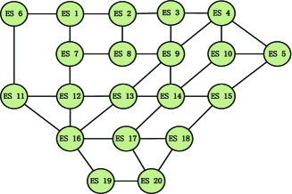
Figure 2: Topology of the server network

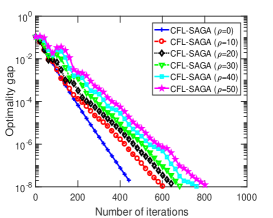
(a) Random graph.

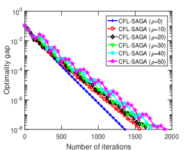
(b) Ring graph.

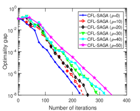
(c) Fully connected graph.

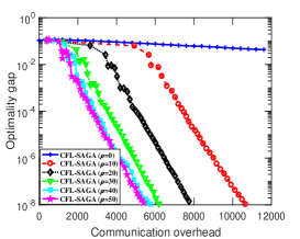
(d) Random graph.

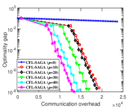
(e) Ring graph.

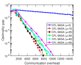
(f) Fully connected graph.

Figure 3: Results on $\ell_{2}$-regularized logistic regression. First row: Optimality gap vs. number of iterations on different server networks; Second row: Optimality gap vs. communication overhead on different server networks

VIII Simulation Results

In this section, we provide simulation results to demonstrate the superiority of the proposed CFL-SAGA algorithm over GT-SAGA and other competing algorithms. We compare the performance of respective algorithms over different user sampling rates as well as different server topologies. We first introduce the experimental settings.

VIII-A Experimental Settings

We consider a CFL system consisting of $N=20$ servers and $400$ users. Each server is assigned to $P_{i}=20$ users. To investigate the performance of respective algorithms over different server topologies, we consider three types of server networks. The first one is a random graph depicted in Fig. 2. The second one is the ring graph (cycle graph), and the last one is a fully connected graph. Since the structures of the ring graph and the fully connected graph are self-evident by their names, we do not draw their topologies for sake of simplicity. Clearly, the fully connected graph has the best connectivity, while the ring graph has the poorest connectivity.

We adopt the $\ell_{2}$-regularized logistic regression problem as our test problem:

$$\mathop{\min}\limits_{\boldsymbol{x}\in\mathbb{R}^{d}} \ \textstyle f(\boldsymbol{x})\triangleq\frac{1}{N}\sum_{i=1}^{N}\sum_{j=1}^{P_{i}}f_{ij}(\boldsymbol{x}),$$ (43)

where $f_{ij}(\boldsymbol{x})=\sum_{t=1}^{S_{ij}}f_{ij,t}(\boldsymbol{x})$,

$$f_{ij,t}(\boldsymbol{x})= \textstyle\sum\limits_{t^{\prime}\in\mathcal{T}_{ij,t}}\Big{(}\frac{\kappa}{2}\|\boldsymbol{x}\|_{2}^{2}-y_{ij,t^{\prime}}\cdot\text{log}\big{(}(1+e^{-\boldsymbol{\omega}_{ij,t^{\prime}}^{T}\boldsymbol{x}})^{-1}\big{)}-$$

$$(1-y_{ij,t^{\prime}})\cdot\text{log}\big{(}1-(1+e^{-\boldsymbol{\omega}_{ij,t^{\prime}}^{T}\boldsymbol{x}})^{-1}\big{)}\Big{)}$$ (44)

in which $\kappa$ is set to $0.05$, $\{\boldsymbol{\omega}_{ij,t^{\prime}}\in\mathbb{R}^{d},y_{ij,t^{\prime}}\in\{0,1\}\}$ is the $t^{\prime}$th training sample stored at user $u_{ij}$, and $\mathcal{T}_{ij,t}$ is the index set of the data samples in the $t$th mini-batch training set. Clearly, $f_{ij,t}$ is strongly convex and its gradient is Lipschitz continuous. In our experiments, both the data vector $\boldsymbol{\omega}_{ij,t^{\prime}}\in\mathbb{R}^{200}$ and the label $y_{ij,t^{\prime}}\in\{0,1\}$ are randomly generated. Each user is assumed to hold $50$ training samples and each mini-batch training set consists of $5$ training samples. As such, the total number of training samples is $20000$.

To evaluate the performance of respective algorithms, we adopt the optimality gap $opg^{k}$ to measure the distance between the current solution and the optimal solution. The optimality gap $opg^{k}$ is defined as $opg^{k}\triangleq\frac{\|\boldsymbol{x}^{k}-\bar{\boldsymbol{W}}_{\infty}\boldsymbol{x}^{*}\|_{2}}{\sqrt{N}}$, where $\boldsymbol{x}^{k}\triangleq[\boldsymbol{x}_{1}^{k};\cdots;\boldsymbol{x}_{N}^{k}]$, $\bar{\boldsymbol{W}}_{\infty}\boldsymbol{x}^{*}\triangleq[\boldsymbol{x}^{*};\cdots;\boldsymbol{x}^{*}]$, and $\boldsymbol{x}^{*}$ is the optimal solution obtained by solving (43) in a centralized manner.

VIII-B Experimental Results

First, we examine the performance of the proposed CFL-SAGA under different choices of the triggering parameter $\rho$ as well as different server topologies. Fig. 3 $(a)$ plots the optimality gap of CFL-SAGA vs. the number of iterations for the random network. The triggering parameter $\rho$ varies from $0$ to $50$. Clearly, $\rho=0$ corresponds to the case of full-uploads, that is, all users are required to upload their VR-SGs in each iteration. In general, we see that the convergence speed of CFL-SAGA becomes slower as $\rho$ increases. This is expected since a larger $\rho$ leads to a smaller number of user uploads, resulting in a larger approximate error in the aggregated gradient. Fig. 3 $(b)$ and $(c)$ plot the optimality gap of CFL-SAGA vs. the number of iterations for the ring graph and the fully connected graph, respectively. For these two server networks, the convergence behavior of CFL-SAGA is similar as that in Fig. 3 $(a)$. Not surprisingly, the algorithm exhibits a faster convergence speed over a more well-connected server network. Fig. 3 $(d)$ plots the optimality gap of CFL-SAGA vs. the communication overhead for the random network. In particular, the communication overhead is measured by the total number of VR-SGs that are uploaded to servers. It is observed that to reach the same accuracy, the required number of user uploads decreases as $\rho$ increases. Nevertheless, our empirical results suggest that the highest communication efficiency is achieved when $\rho=50$, and a larger value of $\rho$ beyond $50$ does not yield further improvement on the communication efficiency. It is also noticed that the CFL-SAGA exhibits a significant advantage in terms of communication efficiency as compared to the full-upload case ($\rho=0$). The reason is that, in distributed optimization, the user gradient usually changes slowly, especially in the high-precision regime. Hence using the stale gradient to generate the aggregated gradient often leads to a very small approximation error. As a result, even with a very small number of user uploads, the algorithm can still maintain a fast convergence speed.

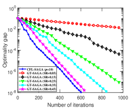
(a) Random graph.

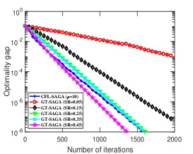
(b) Ring graph.

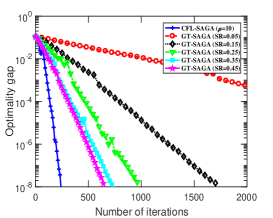
(c) Fully connected graph.

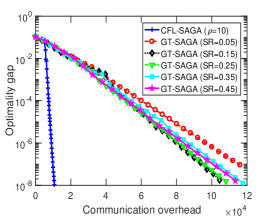
(d) Random graph.

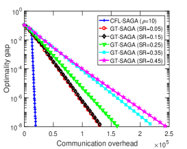
(e) Ring graph.

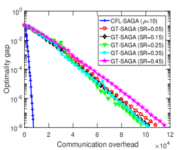
(f) Fully connected graph.

Figure 4: Comparisons on $\ell_{2}$-regularized logistic regression. First row: Optimality gap vs. number of iterations on different server networks; Second row: Optimality gap vs. communication overhead on different server networks. SR is short for ‘Sampling rate’.

Next, we compare the performance of the proposed CFL-SAGA with that of GT-SAGA, namely, Algorithm 2. As shown in Fig. 3, taking $\rho=10$ is sufficient to yield fast convergence as well as high communication efficiency. We thus fix $\rho=10$ for CFL-SAGA. Fig. 4 $(a)$, $(b)$ and $(c)$ plot the optimality gap of respective algorithms vs. the number of iterations for different networks. In Fig. 4 $(a)$, SR is an abbreviation for ‘sampling rate’. For instance, $SR=0.15$ corresponds to the case that $0.15\times 20=3$ users are selected by each server in each iteration. To make a full comparison, the sampling rate of GT-SAGA is tuned from $0.05$ to $0.45$. Clearly, the convergence speed of GT-SAGA becomes faster as the sampling rate increases. It is observed that for the random graph and the fully connected graph, the proposed CFL-SAGA is faster than GT-SAGA that uses a sampling rate as large as $0.45$. As for the communication overhead shown in Fig. 4 $(d)$, $(e)$ and $(f)$, we can see that the proposed CFL-SAGA exhibits higher communication efficiency than GT-SAGA by orders of magnitude. This advantage of CFL-SAGA is mainly due to the fact that the proposed algorithm has the ability of uploading those most informative gradients via the conditionally triggered user selection mechanism, thus reducing the number of uploads substantially without sacrificing the convergence speed of the proposed algorithm. In fact, the averaged number of user uploads per-iteration for our proposed algorithm is even smaller than that of GT-SAGA with a sampling rate of $SR=0.05$.

To examine the computational complexity, we plot in Fig. 5 the average runtime of respective algorithms vs. the number of iterations. We can see that GT-SAGA has a lower per-iteration computational complexity than the CFL-SAGA. This is because for CFL-SAGA, at each iteration each user is required to compute its local stochastic gradient, whether or not this local gradient is uploaded. As a comparison, the GT-SAGA only requires those selected users to compute its stochastic gradient. Note that the computational cost caused by the proposed CTUS mechanism is usually negligible since the CTUS only involves very simple calculations at each user with a complexity scaling linearly with the dimension of the model variable $\boldsymbol{x}$.

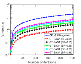
Figure 5: Runtime vs. number of iterations on the random graph

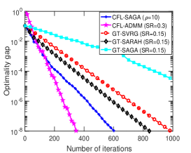
Figure 6: Optimality gap vs. number of iterations on the random graph

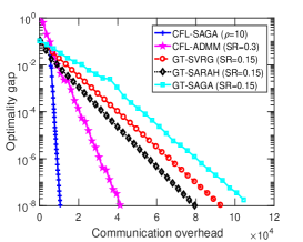
Figure 7: Optimality gap vs. communication overhead on the random graph

At last, we compare the proposed CFL-SAGA with some other state-of-the-art methods, namely, CFL-ADMM [47], GT-SVRG [40] and GT-SARAH [41]. Note that CFL-ADMM randomly selects users to upload their local variables to their respective servers. The user sampling rate of CFL-ADMM is chosen as $0.3$ in our experiments, and $0.15$ for GT-SVRG and GT-SARAG. Recall that both GT-SVRG and GT-SARAH are double-loop based methods. Take GT-SVRG as an example, this algorithms has an outer loop that aims to periodically update the anchor gradient vector, a step very similar to the sum of $\boldsymbol{g}_{ij}^{k+1}$. While the inner iteration is very similar to each iteration of GT-SAGA. For this reason, both GT-SVRG and GT-SARAH can be adapted to the CFL problem in a way similar to GT-SAGA, except that they need to perform a full user upload at the beginning of each outer loop. The parameters for each algorithm is tuned to achieve the best communication efficiency performance. Fig. 6 and Fig. 7 respectively plot the optimality gap and the communication overhead vs. the number of iterations on the random network. Although the other algorithms achieve either similar or even faster convergence speed compared to CFL-SAGA, the proposed CFL-SAGA algorithm exhibits a significant advantage in terms of communication efficiency. This is because the number of per-iteration user uploads of CFL-SAGA is much smaller than those in other algorithms.

IX Conclusion

In this paper, we proposed a SAGA-based method for confederated learning. The proposed method employs conditionally-triggered user selection (CTUS) to achieve communication-efficient learning of the model vector. The major innovation of the proposed method is the use of the CTUS mechanism, which determines whether the user should upload its local VR-SG by measuring its contribution relative to the progress of the algorithm. Thanks to the CTUS mechanism, the proposed algorithm only requires a very small number of uploads to maintain fast convergence. Theoretical analysis indicates that the proposed algorithm enjoys a fast linear convergence and numerical results demonstrate the superior communication efficiency of the proposed algorithm over GT-SAGA.

Appendix A Preliminary Results

First we list some inequalities that will be frequently used in our analysis.

$$\textstyle\|\boldsymbol{x}+\boldsymbol{y}\|_{2}^{2}\leq(1+p^{-1})\|\boldsymbol{x}\|_{2}^{2}+(1+p)\|\boldsymbol{y}\|_{2}^{2},\ \forall p>0,$$ (45)

$$\textstyle\|\sum_{i=1}^{N}\boldsymbol{x}_{i}\|_{2}^{2}\leq N\sum_{i=1}^{N}\|\boldsymbol{x}_{i}\|_{2}^{2}.$$ (46)

$$\text{Variance decomposition}:$$

$$\mathbb{E}\{\|\boldsymbol{x}-\boldsymbol{y}\|_{2}^{2}\}=\mathbb{E}\{\|\boldsymbol{x}-\mathbb{E}\{\boldsymbol{x}\}\|_{2}^{2}\}+\|\mathbb{E}\{\boldsymbol{x}\}-\boldsymbol{y}\|_{2}^{2},\ \forall\boldsymbol{y},$$ (47)

$$\textstyle\mathbb{E}\{\|\frac{1}{N}\sum_{i=1}^{N}(x_{i}-\mathbb{E}\{x_{i}\})\|_{2}^{2}\}=\frac{1}{N^{2}}\mathbb{E}\{\|x_{i}-\mathbb{E}\{x_{i}\}\|_{2}^{2}\},$$

$$\text{with}\ \{x_{i}\}_{i=1}^{N}\ \text{independent of each other}.$$ (48)

Next we present several intermediate results.

Lemma 1 (Lemma 10 in [55]).

Suppose $f$ is $\mu$-strongly convex with its gradient being $L$-Lipschitz continuous. Then for $\forall\boldsymbol{z}\in\mathbb{R}^{d}$, it holds

$$\textstyle\|\boldsymbol{z}-\alpha\nabla f(\boldsymbol{z})-\boldsymbol{z}^{*}\|_{2}\leq(1-\mu\alpha)\|\boldsymbol{z}-\boldsymbol{z}^{*}\|_{2}$$ (49)

where $\boldsymbol{z}^{*}$ is the minimizer of $f$ and $\alpha\leq\frac{1}{L}$ is a constant.

Lemma 2 (Lemma 2 in [56]).

Suppose $\boldsymbol{W}\in\mathbb{R}^{N\times N}$ is primitive and doubly stochastic, then for $\forall\boldsymbol{z}\in\mathbb{R}^{N}$, we have

$$\textstyle\|\boldsymbol{W}\boldsymbol{z}-\boldsymbol{W}_{\infty}\boldsymbol{z}\|_{2}\leq\sigma\|\boldsymbol{z}-\boldsymbol{W}_{\infty}\boldsymbol{z}\|_{2},$$ (50)

where $\sigma$ is the second largest singular value of $\boldsymbol{W}$.

Lemma 3 (Lemma 1 in [57]).

Let the assumptions made in Section II-B hold. Then with $f(\bar{\boldsymbol{x}})=\frac{1}{N}\sum_{i=1}^{N}f_{i}(\bar{\boldsymbol{x}})$ we have

$$\textstyle\|\bar{\nabla}f(\boldsymbol{x})-\nabla f(\bar{\boldsymbol{x}})\|_{2}\leq\frac{L}{\sqrt{N}}\|\boldsymbol{x}-\bar{\boldsymbol{W}}_{\infty}\boldsymbol{x}\|_{2}.$$ (51)

Lemma 4 (Corollary 8.1.29 in [58]).

Suppose $\boldsymbol{T}\in\mathbb{R}^{n\times n}$ is a nonnegative matrix and $\gamma>0$ is a constant. If there exists a positive vector $\boldsymbol{\psi}\in\mathbb{R}^{n}$ such that $\boldsymbol{T}\boldsymbol{\psi}\leq\gamma\boldsymbol{\psi}$, then $\rho(\boldsymbol{T})\leq\gamma$, where $\rho(\boldsymbol{T})\triangleq\max\{|\lambda_{i}|\}$ is the spectral radius of $\boldsymbol{T}$.

At last, we mention that Step $1$ and $5$ in Algorithm 3 can be compactly written as

$$\textstyle\boldsymbol{x}^{k+1}=\bar{\boldsymbol{W}}\boldsymbol{x}^{k}-\alpha\boldsymbol{y}^{k},$$

$$\textstyle\boldsymbol{y}^{k+1}=\bar{\boldsymbol{W}}\boldsymbol{y}^{k}+\boldsymbol{g}^{k+1}-\boldsymbol{g}^{k},$$ (52)

where $\boldsymbol{g}^{k}\triangleq[\boldsymbol{g}_{1}^{k};\cdots;\boldsymbol{g}_{N}^{k}]$.

The left hand side of (40) is the average of $\mathbb{E}_{t_{ij}^{k+1},t_{ij}^{k}}\{\|\boldsymbol{\Delta}_{ij}^{k+1}\|_{2}^{2}\}$s, while $\frac{1}{N}\sum_{i=1}^{N}\|\sum_{i^{\prime}=1}^{N}w_{ii^{\prime}}\boldsymbol{x}_{i^{\prime}}^{k+1}-\boldsymbol{x}_{i}^{k+1}\|_{2}$ in the right hand side of (40) is the average of $\|\sum_{i^{\prime}=1}^{N}w_{ii^{\prime}}\boldsymbol{x}_{i^{\prime}}^{k+1}-\boldsymbol{x}_{i}^{k+1}\|_{2}^{2}$s. The inequality (40) indicates that

$$\textstyle\mathbb{E}_{t_{ij}^{k+1},t_{ij}^{k}}\{\|\boldsymbol{\Delta}_{ij}^{k+1}\|_{2}^{2}\}\lesssim C_{3}\|\sum_{i^{\prime}=1}^{N}w_{ii^{\prime}}\boldsymbol{x}_{i^{\prime}}^{k+1}-\boldsymbol{x}_{i}^{k+1}\|_{2}^{2}$$ (53)

holds in the average sense. As such, if the value of $\rho$ is set to be sufficiently large, then (17) will not be triggered for most of the users. Consequently, the number of uploads can be significantly reduced.

Appendix B Proof of Proposition 1

Without loss of generality, we assume that $t_{ij}^{k+1}\neq t_{ij}^{k}$. Recall that $\boldsymbol{\Delta}_{ij}^{k+1}$ in (15) is defined as $\boldsymbol{\Delta}_{ij}^{k+1}=\boldsymbol{g}_{ij}^{k+1}-\boldsymbol{g}_{ij}^{k}$. Combining this with the definition of $\boldsymbol{g}_{ij}^{k+1}$ we have

$$\boldsymbol{\Delta}_{ij}^{k+1}=S_{ij}\cdot\Big{(}\nabla f_{ij,t_{ij}^{k+1}}(\boldsymbol{x}_{i}^{k+1})-\nabla f_{ij,t_{ij}^{k+1}}(\boldsymbol{\phi}_{ij,t_{ij}^{k+1}}^{k})\Big{)}$$

$$+\nabla f_{ij,t_{ij}^{k}}(\boldsymbol{x}_{i}^{k})-S_{ij}\cdot\Big{(}\nabla f_{ij,t_{ij}^{k}}(\boldsymbol{x}_{i}^{k})-\nabla f_{ij,t_{ij}^{k}}(\boldsymbol{\phi}_{ij,t_{ij}^{k}}^{k})\Big{)}$$

$$-\nabla f_{ij,t_{ij}^{k}}(\boldsymbol{\phi}_{ij,t_{ij}^{k}}^{k})$$

$$=S_{ij}\cdot\Big{(}\nabla f_{ij,t_{ij}^{k+1}}(\boldsymbol{x}_{i}^{k+1})-\nabla f_{ij,t_{ij}^{k+1}}(\boldsymbol{\phi}_{ij,t_{ij}^{k+1}}^{k})\Big{)}$$

$$-(S_{ij}-1)\cdot\Big{(}\nabla f_{ij,t_{ij}^{k}}(\boldsymbol{x}_{i}^{k})-\nabla f_{ij,t_{ij}^{k}}(\boldsymbol{\phi}_{ij,t_{ij}^{k}}^{k})\Big{)}$$

$$\overset{(a)}{=}S_{ij}\cdot\Big{(}\nabla f_{ij,t_{ij}^{k+1}}(\boldsymbol{\phi}_{ij,t_{ij}^{k+1}}^{k+1})-\nabla f_{ij,t_{ij}^{k+1}}(\boldsymbol{\phi}_{ij,t_{ij}^{k+1}}^{k})\Big{)}$$

$$-(S_{ij}-1)\cdot\Big{(}\nabla f_{ij,t_{ij}^{k}}(\boldsymbol{\phi}_{ij,t_{ij}^{k}}^{k+1})-\nabla f_{ij,t_{ij}^{k}}(\boldsymbol{\phi}_{ij,t_{ij}^{k}}^{k})\Big{)},$$ (54)

where in $(a)$ we have used the fact that $\boldsymbol{\phi}_{ij,t_{ij}^{k+1}}^{k+1}=\boldsymbol{x}_{i}^{k+1}$ (resp. $\boldsymbol{\phi}_{ij,t_{ij}^{k}}^{k+1}=\boldsymbol{\phi}_{ij,t_{ij}^{k}}^{k}=\boldsymbol{x}_{i}^{k}$). Combing (54) with the Lipschitz continuity of $f_{ij,t_{ij}^{k}}$ and $f_{ij,t_{ij}^{k+1}}$ we have

$$\|\boldsymbol{\Delta}_{ij}^{k+1}\|_{2}^{2}\leq 2S_{ij}^{2}\cdot L_{ij,t_{ij}^{k+1}}^{2}\cdot\Big{\|}\boldsymbol{\phi}_{ij,t_{ij}^{k+1}}^{k+1}-\boldsymbol{\phi}_{ij,t_{ij}^{k+1}}^{k}\Big{\|}_{2}^{2}$$

$$+2S_{ij}^{2}\cdot L_{ij,t_{ij}^{k}}^{2}\cdot\Big{\|}\boldsymbol{\phi}_{ij,t_{ij}^{k}}^{k+1}-\boldsymbol{\phi}_{ij,t_{ij}^{k}}^{k}\Big{\|}_{2}^{2}$$

$$\leq 4S_{ij}^{2}\cdot L_{ij,t_{ij}^{k+1}}^{2}\cdot\Big{(}\big{\|}\boldsymbol{\phi}_{ij,t_{ij}^{k+1}}^{k+1}-\boldsymbol{x}^{*}\big{\|}_{2}^{2}+\big{\|}\boldsymbol{\phi}_{ij,t_{ij}^{k+1}}^{k}-\boldsymbol{x}^{*}\big{\|}_{2}^{2}\Big{)}$$

$$+4S_{ij}^{2}\cdot L_{ij,t_{ij}^{k}}^{2}\cdot\Big{(}\big{\|}\boldsymbol{\phi}_{ij,t_{ij}^{k}}^{k+1}-\boldsymbol{x}^{*}\big{\|}_{2}^{2}+\big{\|}\boldsymbol{\phi}_{ij,t_{ij}^{k}}^{k}-\boldsymbol{x}^{*}\big{\|}_{2}^{2}\Big{)}.$$ (55)

where $L_{ij,t}$ is the Lipschitz constant corresponding to $\nabla f_{ij,t}$. From (55) we can further deduce that

$$\textstyle\sum\limits_{i=1}^{N}\sum\limits_{j=1}^{P_{i}}\|\boldsymbol{\Delta}_{ij}^{k+1}\|_{2}^{2}\leq\sum\limits_{i=1}^{N}\sum\limits_{j=1}^{P_{i}}4S_{ij}^{2}\Big{(}L_{ij,t_{ij}^{k+1}}^{2}\big{\|}\boldsymbol{\phi}_{ij,t_{ij}^{k+1}}^{k+1}-\boldsymbol{x}^{*}\big{\|}_{2}^{2}+$$

$$\textstyle L_{ij,t_{ij}^{k}}^{2}\big{\|}\boldsymbol{\phi}_{ij,t_{ij}^{k}}^{k+1}-\boldsymbol{x}^{*}\big{\|}_{2}^{2}\Big{)}+\sum\limits_{i=1}^{N}\sum\limits_{j=1}^{P_{i}}4S_{ij}^{2}\Big{(}L_{ij,t_{ij}^{k+1}}^{2}\big{\|}\boldsymbol{\phi}_{ij,t_{ij}^{k+1}}^{k}$$

$$\textstyle-\boldsymbol{x}^{*}\big{\|}_{2}^{2}+L_{ij,t_{ij}^{k}}^{2}\big{\|}\boldsymbol{\phi}_{ij,t_{ij}^{k}}^{k}-\boldsymbol{x}^{*}\big{\|}_{2}^{2}\Big{)}.$$ (56)

which implies that

$$\textstyle\mathbb{E}_{t_{ij}^{k+1},t_{ij}^{k}}\{\sum_{i=1}^{N}\sum_{j=1}^{P_{i}}\|\boldsymbol{\Delta}_{ij}^{k+1}\|_{2}^{2}\}$$

$$\overset{(a)}{\leq}\textstyle 2\sum\limits_{i=1}^{N}\sum\limits_{j=1}^{P_{i}}4S_{ij}^{2}\sum\limits_{t=1}^{S_{ij}}\frac{L_{ij,t}^{2}}{S_{ij}}\Big{(}\big{\|}\boldsymbol{\phi}_{ij,t}^{k+1}-\boldsymbol{x}^{*}\big{\|}_{2}^{2}+\big{\|}\boldsymbol{\phi}_{ij,t}^{k}-\boldsymbol{x}^{*}\big{\|}_{2}^{2}\Big{)}$$

$$\leq 2\bar{L}(D^{k+1}+D^{k})$$ (57)

where

$$\bar{L}=\text{max}\{L_{k+1},L_{k}\},$$

$$\textstyle L_{k+1}=\Big{(}\sum_{i=1}^{N}\sum_{j=1}^{P_{i}}4S_{ij}^{2}\sum_{t=1}^{S_{ij}}\frac{L_{ij,t}^{2}}{S_{ij}}\big{\|}\boldsymbol{\phi}_{ij,t}^{k+1}-\boldsymbol{x}^{*}\big{\|}_{2}^{2}\Big{)}\Big{/}$$

$$\qquad\quad\textstyle\Big{(}\underbrace{\textstyle\sum_{i=1}^{N}\sum_{j=1}^{P_{i}}\sum_{t=1}^{S_{ij}}\big{\|}\boldsymbol{\phi}_{ij,t}^{k+1}-\boldsymbol{x}^{*}\big{\|}_{2}^{2}}_{=D^{k+1}}\Big{)},$$

$$\textstyle L_{k}=\Big{(}\sum_{i=1}^{N}\sum_{j=1}^{P_{i}}4S_{ij}^{2}\sum_{t=1}^{S_{ij}}\frac{L_{ij,t}^{2}}{S_{ij}}\big{\|}\boldsymbol{\phi}_{ij,t}^{k}-\boldsymbol{x}^{*}\big{\|}_{2}^{2}\Big{)}\Big{/}$$

$$\qquad\quad\textstyle\Big{(}\underbrace{\textstyle\sum_{i=1}^{N}\sum_{j=1}^{P_{i}}\sum_{t=1}^{S_{ij}}\big{\|}\boldsymbol{\phi}_{ij,t}^{k}-\boldsymbol{x}^{*}\big{\|}_{2}^{2}}_{D^{k}}\Big{)}.$$ (58)

Taking the full expectation for both sides of (57) yields

$$\textstyle\mathbb{E}\{\sum_{i=1}^{N}\sum_{j=1}^{P_{i}}\|\boldsymbol{\Delta}_{ij}^{k+1}\|_{2}^{2}\}\leq\mathbb{E}\{2\bar{L}(D^{k+1}+D^{k})\}$$

$$\textstyle\approx\mathbb{E}\{4\bar{L}D^{k+1}\}$$

$$\overset{(\ref{lemma5-1-content})}{\leq}\textstyle\mathbb{E}\Big{\{}4\bar{L}\Big{(}(1-\frac{1}{\overline{S_{ij}}})D^{k}+2\overline{P_{i}}X^{k+1}+2\overline{P_{i}}N\bar{X}^{k+1}\Big{)}\Big{\}}$$ (59)

Assuming $\mathbb{E}\{D^{k+1}\}\approx\mathbb{E}\{D^{k}\}$, the above inequality implies that

$$\textstyle\mathbb{E}\{4\bar{L}D^{k+1}\}\leq\mathbb{E}\Big{\{}8\overline{S_{ij}}\bar{L}\overline{P_{i}}\big{(}X^{k+1}+N\bar{X}^{k+1}\big{)}\Big{\}}$$

$$=\mathbb{E}\Big{\{}8\overline{S_{ij}}\bar{L}\overline{P_{i}}\big{(}\|\boldsymbol{x}^{k+1}-\bar{\boldsymbol{W}}_{\infty}\boldsymbol{x}^{k+1}\|_{2}^{2}+\|\bar{\boldsymbol{W}}_{\infty}\boldsymbol{x}^{k+1}-\tilde{\boldsymbol{x}}^{*}\|_{2}^{2}\big{)}\Big{\}}$$

$$\overset{(\ref{theorem2-content-1})}{\leq}\mathbb{E}\Big{\{}8(1+C_{1})\overline{S_{ij}}\bar{L}\overline{P_{i}}\cdot\|\boldsymbol{x}^{k+1}-\bar{\boldsymbol{W}}_{\infty}\boldsymbol{x}^{k+1}\|_{2}^{2}\Big{\}}$$

$$=\mathbb{E}\Big{\{}8(1+C_{1})\overline{S_{ij}}\bar{L}\overline{P_{i}}\cdot\|\boldsymbol{x}^{k+1}-\bar{\boldsymbol{W}}\boldsymbol{x}^{k+1}+\bar{\boldsymbol{W}}\boldsymbol{x}^{k+1}-$$

$$\qquad\qquad\qquad\qquad\qquad\qquad\qquad\qquad\bar{\boldsymbol{W}}_{\infty}\boldsymbol{x}^{k+1}\|_{2}^{2}\Big{\}}$$

$$\leq\mathbb{E}\Big{\{}16(1+C_{1})\overline{S_{ij}}\bar{L}\overline{P_{i}}\big{(}\|\boldsymbol{x}^{k+1}-\bar{\boldsymbol{W}}\boldsymbol{x}^{k+1}\|_{2}^{2}$$

$$\qquad\qquad\qquad\qquad+\|\bar{\boldsymbol{W}}\boldsymbol{x}^{k+1}-\bar{\boldsymbol{W}}_{\infty}\boldsymbol{x}^{k+1}\|_{2}^{2}\big{)}\Big{\}}$$

$$\overset{(\ref{theorem2-content-2})}{\leq}\mathbb{E}\Big{\{}\underbrace{16(1+C_{1})(1+C_{2})\overline{S_{ij}}\bar{L}\overline{P_{i}}}_{[(\ref{comm-effici-4})-1]}\cdot\|\boldsymbol{x}^{k+1}-\bar{\boldsymbol{W}}\boldsymbol{x}^{k+1}\|_{2}^{2}\Big{\}}$$

$$=\textstyle\mathbb{E}\Big{\{}[(\ref{comm-effici-4})-1]\cdot\sum\limits_{i=1}^{N}\big{\|}\sum_{i^{\prime}=1}^{N}w_{ii^{\prime}}\boldsymbol{x}_{i^{\prime}}^{k+1}-\boldsymbol{x}_{i}^{k+1}\big{\|}_{2}^{2}\Big{\}}.$$ (60)

Combining (59) and (60) we obtain

$$\textstyle\mathbb{E}\{\sum_{i=1}^{N}\sum_{j=1}^{P_{i}}\|\boldsymbol{\Delta}_{ij}^{k+1}\|_{2}^{2}\}\overset{(\ref{comm-effici-3-2})}{\lesssim}\mathbb{E}\{4\bar{L}D^{k+1}\}$$

$$\textstyle\overset{(\ref{comm-effici-4})}{\leq}\mathbb{E}\Big{\{}[(\ref{comm-effici-4})-1]\cdot\sum\limits_{i=1}^{N}\big{\|}\sum_{i^{\prime}=1}^{N}w_{ii^{\prime}}\boldsymbol{x}_{i^{\prime}}^{k+1}-\boldsymbol{x}_{i}^{k+1}\big{\|}_{2}^{2}\Big{\}}.$$ (61)

Multiplying $\frac{1}{\sum_{i=1}^{N}P_{i}}$ to both sides of (61) yields the desired result.

Appendix C Proving the First Inequality in (22)

The first inequality, i.e., (62), is proved in the following lemma. For completeness and clarity, we provide a simple proof of this lemma.

Lemma 5 (Lemma 4 in [40]).

Let the assumptions made in Section II-B hold. Then

$$\textstyle X^{k+1}\leq\frac{1+\sigma^{2}}{2}\cdot X^{k}+\frac{2\alpha^{2}}{1-\sigma^{2}}\cdot Y^{k},$$ (62)

$$\textstyle X^{k+1}\leq 2\sigma^{2}\cdot X^{k}+2\alpha^{2}\cdot Y^{k}.$$ (63)

Proof.

According to the first equality of (52), it holds that

$$\textstyle X^{k+1}\overset{(\ref{PropAlg-compact-form})}{=}\|\bar{\boldsymbol{W}}\boldsymbol{x}^{k}-\alpha\boldsymbol{y}^{k}-\bar{\boldsymbol{W}}_{\infty}(\bar{\boldsymbol{W}}\boldsymbol{x}^{k}-\alpha\boldsymbol{y}^{k})\|_{2}^{2}$$

$$\overset{(a)}{\leq} \textstyle(1+p)\|\bar{\boldsymbol{W}}\boldsymbol{x}^{k}-\bar{\boldsymbol{W}}_{\infty}\boldsymbol{x}^{k}\|_{2}^{2}+(1+\frac{1}{p})\alpha^{2}\|\boldsymbol{y}^{k}-\bar{\boldsymbol{W}}_{\infty}\boldsymbol{y}^{k}\|_{2}^{2}$$

$$\overset{(b)}{\leq} \textstyle(1+p)\sigma^{2}\cdot X^{k}+(1+\frac{1}{p})\alpha^{2}\cdot Y^{k},\ \forall p>0,$$ (64)

where $(a)$ is because $\bar{\boldsymbol{W}}_{\infty}\bar{\boldsymbol{W}}=\bar{\boldsymbol{W}}_{\infty}$ as well as (45), and $(b)$ comes from Lemma 2 (note that $\boldsymbol{W}$ and $\bar{\boldsymbol{W}}$ shares similar properties because $\bar{\boldsymbol{W}}\triangleq\boldsymbol{W}\otimes\boldsymbol{I}_{d}$). Setting $p=\frac{1-\sigma^{2}}{2\sigma^{2}}$ (resp. $1$) and using $\sigma<1$ leads to (62) (resp. (63)). ∎

Appendix D Proving the Second Inequality in (22)

Before starting, we introduce several notations that will be used later. let $\mathcal{F}^{k}=\{t_{ij}^{k^{\prime}}\}_{i,j,k^{\prime}=1}^{i=N,j=P_{i},k^{\prime}=k}$ denote the set of random variables appeared before the $(k+1)$th iteration. Also let $\mathbb{E}^{\mathcal{F}^{k}}\{\cdot\}$ represent the conditional expectation that is conditioned on $\mathcal{F}^{k}$. At last, we use $r^{k}$ to refer to $\{t_{ij}^{k}\}_{i=1,j=1}^{i=N,j=P_{i}}$, which is the set of random variables in the $k$th iteration. The second inequality in (22) reads as follows

$$\textstyle\mathbb{E}\{\bar{X}^{k+1}\}\leq\mathbb{E}\{b_{1}\cdot\bar{X}^{k}+b_{2}\cdot X^{k}+b_{3}\cdot D^{k-1}\}$$ (65)

We will prove this inequality in Lemma 7. Before presenting Lemma 7, we first provide an important intermediate result.

Lemma 6.

Suppose the assumptions in Section II-B hold. Let $(\boldsymbol{x}^{k},\boldsymbol{y}^{k})$ be generated by the proposed Algorithm 3. Then

$$\textstyle\mathbb{E}\{\|\boldsymbol{g}^{k}-\nabla f(\boldsymbol{x}^{k})\|_{2}^{2}\}\leq\textstyle\mathbb{E}\{c_{1}X^{k}+c_{2}\bar{X}^{k}+c_{3}D^{k-1}\},$$ (66)

where $\nabla f(\boldsymbol{x}^{k})\triangleq[\nabla f_{1}(\boldsymbol{x}_{1}^{k});\cdots;\nabla f_{N}(\boldsymbol{x}_{N}^{k})]$, $\boldsymbol{g}^{k}\triangleq[\boldsymbol{g}_{1}^{k};\cdots;\boldsymbol{g}_{N}^{k}]$, $\boldsymbol{g}_{i}^{k}$ is defined in Algorithm 3,

$$\textstyle c_{1}\triangleq 8L^{2}(1+\overline{P_{i}}\cdot\overline{S_{ij}}^{2})+12\rho(1+\sigma^{2})\overline{P_{i}}^{2},$$

$$\textstyle c_{2}\triangleq 8L^{2}(1+\overline{P_{i}}\cdot\overline{S_{ij}}^{2})N,\ c_{3}\triangleq 4L^{2}\overline{S_{ij}},$$ (67)

$\overline{P_{i}}\triangleq\max_{i}\{P_{i}\}$ and $\overline{S_{ij}}=\max_{i,j}\{S_{ij}\}$.

Proof.

For notational convenience, denote $G^{k}=\|\boldsymbol{g}^{k}-\nabla f(\boldsymbol{x}^{k})\|_{2}^{2}$ and $G_{i}^{k}=\|\boldsymbol{g}_{i}^{k}-\nabla f_{i}(\boldsymbol{x}^{k})\|_{2}^{2}$. Since $\mathbb{E}\{G^{k}\}=\mathbb{E}\{\sum_{i=1}^{N}G_{i}^{k}\}$, we should separately bound each $\mathbb{E}\{G_{i}^{k}\}$. For this term, we first consider its conditional expectation:

$$\textstyle\mathbb{E}_{r^{k}}^{\mathcal{F}^{k-1}}\{G_{i}^{k}\}\overset{(a)}{=}\mathbb{E}_{r^{k}}^{\mathcal{F}^{k-1}}\Big{\{}\Big{\|}\boldsymbol{g}_{i}^{k}-\mathbb{E}_{r^{k}}^{\mathcal{F}^{k-1}}\{\boldsymbol{g}_{i}^{k}+\sum\limits_{j\in\mathcal{N}_{i}^{k}}\boldsymbol{\Delta}_{ij}^{k}\}\Big{\|}_{2}^{2}\Big{\}}$$

$$\textstyle\overset{(\ref{def-multi-vect-inequal})}{\leq}2\mathbb{E}_{r^{k}}^{\mathcal{F}^{k-1}}\Big{\{}\|\boldsymbol{g}_{i}^{k}-\mathbb{E}_{r^{k}}^{\mathcal{F}^{k-1}}\{\boldsymbol{g}_{i}^{k}\}\|_{2}^{2}+\big{\|}\mathbb{E}_{r^{k}}^{\mathcal{F}^{k-1}}\big{\{}\sum\limits_{j\in\mathcal{N}_{i}^{k}}\boldsymbol{\Delta}_{ij}^{k}\big{\}}\big{\|}_{2}^{2}\Big{\}}$$

$$\textstyle\overset{(b)}{\leq}2\mathbb{E}_{r^{k}}^{\mathcal{F}^{k-1}}\{\|\boldsymbol{g}_{i}^{k}-\nabla f_{i}(\boldsymbol{x}^{*})\|_{2}^{2}+\textstyle\|\sum_{j\in\mathcal{N}_{i}^{k}}\boldsymbol{\Delta}_{ij}^{k}\|_{2}^{2}\},$$ (68)

where $(a)$ follows from

$$\textstyle\mathbb{E}_{r^{k}}^{\mathcal{F}^{k-1}}\{\boldsymbol{g}_{i}^{k}+\sum_{j\in\mathcal{N}_{i}^{k}}\boldsymbol{\Delta}_{ij}^{k}\}$$

$$\textstyle\overset{(\ref{main-alg-3})}{=}\mathbb{E}_{r^{k}}^{\mathcal{F}^{k-1}}\{\textstyle\sum_{j=1}^{P_{i}}(\boldsymbol{g}_{ij}^{k-1}+\boldsymbol{\Delta}_{ij}^{k})\}=\textstyle\nabla f_{i}(\boldsymbol{x}^{k}),$$ (69)

$(b)$ has invoked (47) for the first term (by treating $\nabla f_{i}(\boldsymbol{x}^{*})$ as $\boldsymbol{y}$) and Jensen’s inequality for the second term. Regarding $\|\sum_{j\in\mathcal{N}_{i}^{k}}\boldsymbol{\Delta}_{ij}^{k}\|_{2}^{2}$ in the last line of (68), we have

$$\mathbb{E}_{r^{k}}^{\mathcal{F}^{k-1}}\{\textstyle\|\sum_{j\in\mathcal{N}_{i}^{k}}\boldsymbol{\Delta}_{ij}^{k}\|_{2}^{2}\}\overset{(\ref{def-multi-vect-inequal})}{\leq}\mathbb{E}_{r^{k}}^{\mathcal{F}^{k-1}}\{|\mathcal{N}_{i}^{k}|\sum_{j\in\mathcal{N}_{i}^{k}}\|\boldsymbol{\Delta}_{ij}^{k}\|_{2}^{2}\}$$

$$\textstyle\overset{(a)}{\leq}|\mathcal{N}_{i}^{k}|^{2}\rho\|\boldsymbol{x}_{i}^{k}-[\bar{\boldsymbol{W}}]_{i}\boldsymbol{x}^{k}\|_{2}^{2},$$ (70)

where $[\bar{\boldsymbol{W}}]_{i}$ represents the $i$th block-row of $\bar{\boldsymbol{W}}$, and $(a)$ comes from Step 3.2 of Algorithm 3. Substituting (70) into (68) yields

$$\textstyle\mathbb{E}_{r^{k}}^{\mathcal{F}^{k-1}}\{G_{i}^{k}\}$$

$$\textstyle\leq\mathbb{E}_{r^{k}}^{\mathcal{F}^{k-1}}\{2\|\boldsymbol{g}_{i}^{k}-\nabla f_{i}(\boldsymbol{x}^{*})\|_{2}^{2}\}+2|\mathcal{N}_{i}^{k}|^{2}\rho\|\boldsymbol{x}_{i}^{k}-[\bar{\boldsymbol{W}}]_{i}\boldsymbol{x}^{k}\|_{2}^{2}$$

$$\overset{(\ref{def-VD})}{=}\textstyle 2|\mathcal{N}_{i}^{k}|^{2}\rho\|\boldsymbol{x}_{i}^{k}-[\bar{\boldsymbol{W}}]_{i}\boldsymbol{x}^{k}\|_{2}^{2}+2\underbrace{\textstyle\mathbb{E}_{r^{k}}^{\mathcal{F}^{k-1}}\{\|\boldsymbol{g}_{i}^{k}-\mathbb{E}_{r^{k}}^{\mathcal{F}^{k-1}}\{\boldsymbol{g}_{i}^{k})\|_{2}^{2}\}}_{\triangleq T_{2}}$$

$$\textstyle+2\underbrace{\textstyle\|\mathbb{E}_{r^{k}}^{\mathcal{F}^{k-1}}\{\boldsymbol{g}_{i}^{k}\}-\nabla f_{i}(\boldsymbol{x}^{*})\|_{2}^{2}}_{\triangleq T_{1}}.$$ (71)

We next separately bound $T_{1}$ and $T_{2}$. For $T_{1}$ we have

$$T_{1}=\textstyle\|\mathbb{E}_{r^{k}}^{\mathcal{F}^{k-1}}\{\boldsymbol{g}_{i}^{k}+\sum_{j\in\mathcal{N}_{i}^{k}}(\boldsymbol{\Delta}_{ij}^{k}-\boldsymbol{\Delta}_{ij}^{k})\}-\nabla f_{i}(\boldsymbol{x}^{*})\|_{2}^{2}$$

$$\overset{(a)}{\leq}\textstyle 2\|\nabla f_{i}(\boldsymbol{x}_{i}^{k})-\nabla f_{i}(\boldsymbol{x}^{*})\|_{2}^{2}+2\|\mathbb{E}_{r^{k}}^{\mathcal{F}^{k-1}}\{\sum_{j\in\mathcal{N}_{i}^{k}}\boldsymbol{\Delta}_{ij}^{k}\}\|_{2}^{2}$$

$$\overset{(b)}{\leq}\textstyle 2L^{2}\|\boldsymbol{x}_{i}^{k}-\boldsymbol{x}^{*}\|_{2}^{2}+2\mathbb{E}_{r^{k}}^{\mathcal{F}^{k-1}}\{|\mathcal{N}_{i}^{k}|\sum_{j\in\mathcal{N}_{i}^{k}}\|\boldsymbol{\Delta}_{ij}^{k}\|_{2}^{2}\}$$

$$\overset{(\ref{lemmaX-2})}{\leq}\textstyle 2L^{2}\|\boldsymbol{x}_{i}^{k}-\boldsymbol{x}^{*}\|_{2}^{2}+2|\mathcal{N}_{i}^{k}|^{2}\rho\|\boldsymbol{x}_{i}^{k}-[\bar{\boldsymbol{W}}]_{i}\boldsymbol{x}^{k}\|_{2}^{2},$$ (72)

where $(a)$ has used (69) and (45), $(b)$ has invoked the Lipschitz continuity of $\nabla f_{i}$ and Jensen’s inequality. For $T_{2}$ it holds that

$$T_{2}\overset{(\ref{main-alg-3})}{=}\textstyle\mathbb{E}_{r^{k}}^{\mathcal{F}^{k-1}}\{\|\sum_{j\notin\mathcal{N}_{i}^{k}}\boldsymbol{g}_{ij}^{k}-\mathbb{E}_{r^{k}}^{\mathcal{F}^{k-1}}\{\sum_{j\notin\mathcal{N}_{i}^{k}}\boldsymbol{g}_{ij}^{k}\}\|_{2}^{2}\}$$

$$\overset{(\ref{def-expectation-equal})}{=}\textstyle\mathbb{E}_{r^{k}}^{\mathcal{F}^{k-1}}\{\sum_{j\notin\mathcal{N}_{i}^{k}}\|\boldsymbol{g}_{ij}^{k}-\mathbb{E}_{r^{k}}^{\mathcal{F}^{k-1}}\{\boldsymbol{g}_{ij}^{k}\}\|_{2}^{2}\},$$

$$\leq\textstyle\mathbb{E}_{\{t_{ij}^{k}\}}^{\mathcal{F}^{k-1}}\{\textstyle\sum_{j=1}^{P_{i}}\|\boldsymbol{g}_{ij}^{k}-\mathbb{E}_{t_{ij}^{k}}^{\mathcal{F}^{k-1}}\{\boldsymbol{g}_{ij}^{k}\}\|_{2}^{2}\}$$

$$\textstyle\overset{(a)}{=}\textstyle\textstyle\sum_{j=1}^{P_{i}}\mathbb{E}_{\{t_{ij}^{k}\}}^{\mathcal{F}^{k-1}}\Big{\{}\Big{\|}S_{ij}\cdot\Big{(}\nabla f_{ij,t_{ij}^{k}}(\boldsymbol{x}_{i}^{k})-\nabla f_{ij,t_{ij}^{k}}(\boldsymbol{\phi}_{ij,t_{ij}^{k}}^{k-1})$$

$$\textstyle\qquad\qquad\quad-\mathbb{E}_{t_{ij}^{k}}^{\mathcal{F}^{k-1}}\big{\{}\nabla f_{ij,t_{ij}^{k}}(\boldsymbol{x}_{i}^{k})-\nabla f_{ij,t_{ij}^{k}}(\boldsymbol{\phi}_{ij,t_{ij}^{k}}^{k-1})\big{\}}\Big{)}\Big{\|}_{2}^{2}\Big{\}}$$

$$\overset{(\ref{def-VD})}{\leq}\textstyle\textstyle\sum_{j=1}^{P_{i}}S_{ij}^{2}\cdot\mathbb{E}_{t_{ij}^{k}}^{\mathcal{F}^{k-1}}\Big{\{}\|\nabla f_{ij,t_{ij}^{k}}(\boldsymbol{x}_{i}^{k})-\nabla f_{ij,t_{ij}^{k}}(\boldsymbol{\phi}_{ij,t_{ij}^{k}}^{k-1})\|_{2}^{2}\Big{\}}$$

$$=\textstyle\textstyle\sum_{j=1}^{P_{i}}S_{ij}\sum_{t=1}^{S_{ij}}\|\nabla f_{ij,t}(\boldsymbol{x}_{i}^{k})-\nabla f_{ij,t}(\boldsymbol{\phi}_{ij,t}^{k-1})\|_{2}^{2}$$

$$\overset{(b)}{\leq}\textstyle\textstyle\sum\limits_{j=1}^{P_{i}}2L^{2}S_{ij}\sum\limits_{t=1}^{S_{ij}}\Big{(}\|\boldsymbol{x}_{i}^{k}-\boldsymbol{x}^{*}\|_{2}^{2}+\|\boldsymbol{x}^{*}-\boldsymbol{\phi}_{ij,t}^{k-1}\|_{2}^{2}\Big{)},$$ (73)

where $(a)$ used the definition of $\boldsymbol{g}_{ij}^{k}$ and the fact that $\mathbb{E}_{t_{ij}^{k}}^{\mathcal{F}^{k-1}}\{\boldsymbol{g}_{ij}^{k}\}=\nabla f_{ij}(\boldsymbol{x}_{i}^{k})=S_{ij}\cdot\mathbb{E}_{t_{ij}^{k}}^{\mathcal{F}^{k-1}}\{\nabla f_{ij,t_{ij}^{k}}(\boldsymbol{x}_{i}^{k})\}$, and $(b)$ used the Lipschitz continuity of $\nabla f_{ij,t}$ as well as (46). Substituting (72) and (73) into (71) yields

$$\textstyle\mathbb{E}_{r^{k}}^{\mathcal{F}^{k-1}}\{G^{k}\}=\mathbb{E}_{r^{k}}^{\mathcal{F}^{k-1}}\{\sum_{i=1}^{N}G_{i}^{k}\}$$

$$\leq\textstyle\sum_{i=1}^{N}\big{(}4L^{2}(1+P_{i}S_{ij}^{2})\|\boldsymbol{x}_{i}^{k}-\boldsymbol{x}^{*}\|_{2}^{2}+$$

$$\textstyle\sum\limits_{j=1}^{P_{i}}4L^{2}S_{ij}\sum\limits_{t=1}^{S_{ij}}\|\boldsymbol{x}^{*}-\boldsymbol{\phi}_{ij,t}^{k-1}\|_{2}^{2}+6|\mathcal{N}_{i}^{k}|^{2}\rho\|\boldsymbol{x}_{i}^{k}-[\bar{\boldsymbol{W}}]_{i}\boldsymbol{x}^{k}\|_{2}^{2}\big{)}$$

$$\leq\textstyle\sum_{i=1}^{N}8L^{2}(1+P_{i}S_{ij}^{2})(\|\bar{\boldsymbol{x}}^{k}-\boldsymbol{x}^{*}\|_{2}^{2}+\|\boldsymbol{x}_{i}^{k}-\bar{\boldsymbol{x}}^{k}\|_{2}^{2})$$

$$\textstyle\qquad+4L^{2}\overline{S_{ij}}\cdot D^{k-1}+6\overline{P_{i}}^{2}\rho\|\boldsymbol{x}^{k}-\bar{\boldsymbol{W}}\boldsymbol{x}^{k}\|_{2}^{2},$$

$$\overset{(a)}{\leq}\textstyle c_{2}\bar{X}^{k}+c_{1}X^{k}+c_{3}D^{k-1},$$ (74)

where $\overline{S_{ij}}=\max_{i,j}\{S_{ij}\}$, $\overline{P_{i}}\triangleq\max_{i}\{P_{i}\}$, $\{c_{i}\}_{i=1}^{3}$ are defined in (67), and $(a)$ is because

$$\textstyle\|\boldsymbol{x}^{k}-\bar{\boldsymbol{W}}\boldsymbol{x}^{k}\|_{2}^{2}\leq 2\|\boldsymbol{x}^{k}-\bar{\boldsymbol{W}}_{\infty}\boldsymbol{x}^{k}\|_{2}^{2}+2\|\bar{\boldsymbol{W}}\boldsymbol{x}^{k}-\bar{\boldsymbol{W}}_{\infty}\boldsymbol{x}^{k}\|_{2}^{2}$$

$$\textstyle\overset{\text{Lemma}\ \ref{lemma2}}{\leq}2(1+\sigma^{2})\|\boldsymbol{x}^{k}-\bar{\boldsymbol{W}}_{\infty}\boldsymbol{x}^{k}\|_{2}^{2}=2(1+\sigma^{2})X^{k}.$$ (75)

Taking a full expectation for both sides of (74) yields (66). ∎

With the help of Lemma 6, we can proceed to prove (65).

Lemma 7.

Suppose the assumptions in Section II-B hold. Let $(\boldsymbol{x}^{k+1},\boldsymbol{y}^{k+1})$ be generated by the proposed Algorithm 3. It is also assumed that $\alpha\leq\frac{1}{L}$ and $\boldsymbol{y}^{0}=\boldsymbol{g}^{0}=\boldsymbol{0}$. Then the following inequalities hold:

$$\textstyle\mathbb{E}\{\bar{X}^{k+1}\}\leq\mathbb{E}\{b_{1}\cdot\bar{X}^{k}+b_{2}\cdot X^{k}+b_{3}\cdot D^{k-1}\}$$ (76)

$$\textstyle\mathbb{E}\{\bar{X}^{k+1}\}\leq\mathbb{E}\{(2+\frac{2c_{1}}{L^{2}})\cdot\bar{X}^{k}+\bar{b}\cdot X^{k}+b_{3}\cdot D^{k-1}\}$$ (77)

where

$$\textstyle b_{1}=1-\mu\alpha+\frac{2c_{2}\alpha^{2}}{N},b_{2}=\frac{2\alpha L^{2}+4\alpha\rho(1+\sigma^{2})\overline{P_{i}}^{2}+2\mu\alpha^{2}L^{2}+2\mu\alpha^{2}c_{1}}{\mu N},$$

$$\textstyle b_{3}=\frac{2\alpha^{2}c_{3}}{N},\ \bar{b}=\frac{4\alpha^{2}L^{2}+4\alpha^{2}\rho(1+\sigma^{2})\overline{P_{i}}^{2}+2\alpha^{2}c_{1}}{N}.$$ (78)

Comment 1.

Note that (76) is the second inequality in (22). While the inequality (77) will be used in Lemma 9.

Proof.

Define $\bar{\boldsymbol{g}}^{k}\triangleq\frac{1}{N}(\boldsymbol{1}_{N}^{T}\otimes\boldsymbol{I}_{d})\boldsymbol{g}^{k}$ as the average of $\boldsymbol{g}^{k}_{i}$s. Since $\boldsymbol{y}^{0}=\boldsymbol{g}^{0}=\boldsymbol{0}$, according to (52) it holds that

$$\textstyle\boldsymbol{y}^{1}\overset{(\ref{PropAlg-compact-form})}{=}\bar{\boldsymbol{W}}\boldsymbol{y}^{0}+\boldsymbol{g}^{1}-\boldsymbol{g}^{0}\Rightarrow\boldsymbol{y}^{1}=\boldsymbol{g}^{1}$$

$$\textstyle\Rightarrow\bar{\boldsymbol{W}}_{\infty}\boldsymbol{y}^{2}\overset{(\ref{PropAlg-compact-form})}{=}\bar{\boldsymbol{W}}_{\infty}(\bar{\boldsymbol{W}}\boldsymbol{y}^{1}+\boldsymbol{g}^{2}-\boldsymbol{y}^{1})\overset{(a)}{\Rightarrow}\bar{\boldsymbol{y}}^{2}=\bar{\boldsymbol{g}}^{2}$$ (79)

where $(a)$ is because $\bar{\boldsymbol{W}}_{\infty}\boldsymbol{y}^{2}=\bar{\boldsymbol{y}}^{2}$, $\bar{\boldsymbol{W}}_{\infty}\bar{\boldsymbol{W}}=\bar{\boldsymbol{W}}_{\infty}$ and $\bar{\boldsymbol{W}}_{\infty}\boldsymbol{g}^{2}=\bar{\boldsymbol{g}}^{2}$. Using deduction we have

$$\bar{\boldsymbol{g}}^{k}=\bar{\boldsymbol{y}}^{k},\ \forall k.$$ (80)

Multiplying $\frac{\boldsymbol{1}_{N}^{T}\otimes\boldsymbol{I}_{d}}{N}$ to the first line of (52) yields

$$\bar{\boldsymbol{x}}^{k+1}\overset{(a)}{=}\bar{\boldsymbol{x}}^{k}-\alpha\bar{\boldsymbol{y}}^{k}\overset{(b)}{=}\bar{\boldsymbol{x}}^{k}-\alpha\bar{\boldsymbol{g}}^{k}$$ (81)

where $(a)$ is because $\frac{\boldsymbol{1}_{N}^{T}\otimes\boldsymbol{I}_{d}}{N}\bar{\boldsymbol{W}}=\frac{\boldsymbol{1}_{N}^{T}\otimes\boldsymbol{I}_{d}}{N}$ ($\boldsymbol{W}$ is doubly stochastic), and $(b)$ is because $\bar{\boldsymbol{g}}^{k}=\bar{\boldsymbol{y}}^{k}$. Then we have

$$\textstyle\mathbb{E}_{r^{k}}^{\mathcal{F}^{k-1}}\{\bar{X}^{k+1}\}\overset{(\ref{appendix-a-1})}{=}\mathbb{E}_{r^{k}}^{\mathcal{F}^{k-1}}\{\|\bar{\boldsymbol{x}}^{k}-\alpha\bar{\boldsymbol{g}}^{k}-\boldsymbol{x}^{*}\|_{2}^{2}\}$$

$$=\textstyle\mathbb{E}_{r^{k}}^{\mathcal{F}^{k-1}}\{\|\bar{\boldsymbol{x}}^{k}-\alpha\nabla f(\bar{\boldsymbol{x}}^{k})+\alpha\nabla f(\bar{\boldsymbol{x}}^{k})-\alpha\bar{\boldsymbol{g}}^{k}-\boldsymbol{x}^{*}\|_{2}^{2}\}$$

$$=\textstyle\|\bar{\boldsymbol{x}}^{k}-\boldsymbol{x}^{*}-\alpha\nabla f(\bar{\boldsymbol{x}}^{k})\|_{2}^{2}+\mathbb{E}_{r^{k}}^{\mathcal{F}^{k-1}}\Big{\{}\alpha^{2}\underbrace{\|\nabla f(\bar{\boldsymbol{x}}^{k})-\bar{\boldsymbol{g}}^{k}\|_{2}^{2}}_{\text{[(\ref{appendix-a-2})-2]}}$$

$$\textstyle+2\alpha\underbrace{\langle\bar{\boldsymbol{x}}^{k}-\boldsymbol{x}^{*}-\alpha\nabla f(\bar{\boldsymbol{x}}^{k}),\nabla f(\bar{\boldsymbol{x}}^{k})-\bar{\boldsymbol{g}}^{k}\rangle}_{\text{[(\ref{appendix-a-2})-1]}}\Big{\}}$$

$$\overset{(a)}{\leq}\textstyle(1-\mu\alpha)^{2}\bar{X}^{k}+\mathbb{E}_{r^{k}}^{\mathcal{F}^{k-1}}\{2\alpha\text{[(\ref{appendix-a-2})-1]}+\alpha^{2}\text{[(\ref{appendix-a-2})-2]}\}$$ (82)

where $(a)$ invoked Lemma 1.

D-1 Bounding [(82)-1] and [(82)-2]

Regarding the term [(82)-1], we have

$$\mathbb{E}_{r^{k}}^{\mathcal{F}^{k-1}}\{\text{[(\ref{appendix-a-2})-1]}\}$$

$$\textstyle=\mathbb{E}_{r^{k}}^{\mathcal{F}^{k-1}}\{\langle\underbrace{\bar{\boldsymbol{x}}^{k}-\boldsymbol{x}^{*}-\alpha\nabla f(\bar{\boldsymbol{x}}^{k})}_{\text{[(\ref{appendix-a-4})-1]}},\nabla f(\bar{\boldsymbol{x}}^{k})-\bar{\boldsymbol{g}}^{k}\rangle\}$$

$$=\textstyle\mathbb{E}_{r^{k}}^{\mathcal{F}^{k-1}}\Big{\{}\langle\text{[(\ref{appendix-a-4})-1]},\nabla f(\bar{\boldsymbol{x}}^{k})-\bar{\nabla}f(\boldsymbol{x}^{k})\rangle+$$

$$\textstyle\qquad\langle\text{[(\ref{appendix-a-4})-1]},\bar{\nabla}f(\boldsymbol{x}^{k})-(\bar{\boldsymbol{g}}^{k}+\frac{1}{N}\sum_{i=1}^{N}\sum_{j\in\mathcal{N}_{i}^{k}}\boldsymbol{\Delta}_{ij}^{k})\rangle$$

$$\qquad\qquad+\textstyle\underbrace{\textstyle\langle\text{[(\ref{appendix-a-4})-1]},\frac{1}{N}\sum_{i=1}^{N}\sum_{j\in\mathcal{N}_{i}^{k}}\boldsymbol{\Delta}_{ij}^{k}\rangle}_{\text{[(\ref{appendix-a-4})-2]}}\Big{\}}$$

$$\overset{(a)}{\leq}\textstyle\mathbb{E}_{r^{k}}^{\mathcal{F}^{k-1}}\{\|\text{[(\ref{appendix-a-4})-1]}\|_{2}\cdot\|\nabla f(\bar{\boldsymbol{x}}^{k})-\bar{\nabla}f(\boldsymbol{x}^{k})\|_{2}+\text{[(\ref{appendix-a-4})-2]}\}$$

$$\overset{(b)}{\leq}\textstyle\mathbb{E}_{r^{k}}^{\mathcal{F}^{k-1}}\{(1-\mu\alpha)\bar{X}^{k}\cdot\|\nabla f(\bar{\boldsymbol{x}}^{k})-\bar{\nabla}f(\boldsymbol{x}^{k})\|_{2}+\text{[(\ref{appendix-a-4})-2]}\}$$

$$\overset{(c)}{\leq}\textstyle\mathbb{E}_{r^{k}}^{\mathcal{F}^{k-1}}\Big{\{}\frac{p(1-\mu\alpha)}{2}\bar{X}^{k}+\frac{(1-\mu\alpha)}{2p}\|\nabla f(\bar{\boldsymbol{x}}^{k})-\bar{\nabla}f(\boldsymbol{x}^{k})\|_{2}^{2}$$

$$\textstyle\qquad\qquad+\text{[(\ref{appendix-a-4})-2]}\Big{\}}$$

$$\overset{(d)}{\leq}\textstyle\mathbb{E}_{r^{k}}^{\mathcal{F}^{k-1}}\big{\{}\frac{p(1-\mu\alpha)}{2}\bar{X}^{k}+\frac{L^{2}}{2pN}X^{k}+\text{[(\ref{appendix-a-4})-2]}\big{\}},\forall p>0,$$ (83)

where $\bar{\nabla}f(\boldsymbol{x})=\frac{1}{N}(\boldsymbol{1}_{N}^{T}\otimes\boldsymbol{I}_{d})\nabla f(\boldsymbol{x})$ is the average of $\nabla f_{i}(\boldsymbol{x}_{i})$s, and $(a)$ has invoked the Cauchy-Schwarz inequality as well as the fact that

$$\textstyle\mathbb{E}_{r^{k}}^{\mathcal{F}^{k-1}}\{\bar{\nabla}f(\boldsymbol{x}^{k})-(\bar{\boldsymbol{g}}^{k}+\frac{1}{N}\sum_{i=1}^{N}\sum_{j\in\mathcal{N}_{i}^{k}}\boldsymbol{\Delta}_{ij}^{k})\}=\boldsymbol{0},$$

$(b)$ used Lemma 1, $(c)$ uses the inequality $\langle\boldsymbol{x},\boldsymbol{y}\rangle\leq\frac{p}{2}\|\boldsymbol{x}\|_{2}^{2}+\frac{1}{2p}\|\boldsymbol{y}\|_{2}^{2}$, $\forall p>0$, and $(d)$ invoked Lemma 3 as well as $1-\mu\alpha<1$. For [(83)-2] we have

$$\textstyle\mathbb{E}_{r^{k}}^{\mathcal{F}^{k-1}}\{\text{[(\ref{appendix-a-4})-2]}\}\overset{(a)}{\leq}\mathbb{E}_{r^{k}}^{\mathcal{F}^{k-1}}\Big{\{}(1-\mu\alpha)\bar{X}^{k}\|\frac{1}{N}\sum\limits_{i=1}^{N}\sum\limits_{j\in\mathcal{N}_{i}^{k}}\boldsymbol{\Delta}_{ij}^{k}\|_{2}\Big{\}}$$

$$\textstyle\leq\frac{p(1-\mu\alpha)}{2}\bar{X}^{k}+\mathbb{E}_{r^{k}}^{\mathcal{F}^{k-1}}\Big{\{}\frac{(1-\mu\alpha)}{2p}\|\frac{1}{N}\sum_{i=1}^{N}\sum_{j\in\mathcal{N}_{i}^{k}}\boldsymbol{\Delta}_{ij}^{k}\|_{2}^{2}\Big{\}}$$

$$\overset{(b)}{\leq}\textstyle\frac{p(1-\mu\alpha)}{2}\bar{X}^{k}+\frac{1}{2pN}\sum_{i=1}^{N}P_{i}\sum_{j=1}^{P_{i}}\rho\|\boldsymbol{x}_{i}^{k}-[\bar{\boldsymbol{W}}]_{i}\boldsymbol{x}^{k}\|_{2}^{2}$$

$$\textstyle\overset{(\ref{lemmaX-14})}{\leq}\textstyle\frac{p(1-\mu\alpha)}{2}\bar{X}^{k}+\frac{\rho(1+\sigma^{2})\overline{P_{i}}^{2}}{pN}X^{k},\ \forall p>0,$$ (84)

where $(a)$ has invoked the Cauchy-Schwarz inequality as well as Lemma 1, and $(b)$ used (46) and (70). As for [(82)-2], we have

$$\textstyle\mathbb{E}_{r^{k}}^{\mathcal{F}^{k-1}}\{\text{[(\ref{appendix-a-2})-2]}\}$$

$$\textstyle\overset{(\ref{def-triangle-inequal})}{\leq}\textstyle 2\|\nabla f(\bar{\boldsymbol{x}}^{k})-\bar{\nabla}f(\boldsymbol{x}^{k})\|_{2}^{2}+\mathbb{E}_{r^{k}}^{\mathcal{F}^{k-1}}\{2\|\bar{\nabla}f(\boldsymbol{x}^{k})-\bar{\boldsymbol{g}}^{k}\|_{2}^{2}\}$$

$$\overset{(a)}{\leq}\textstyle\frac{2L^{2}}{N}X^{k}+\mathbb{E}_{r^{k}}^{\mathcal{F}^{k-1}}\{\frac{2}{N}\sum_{i=1}^{N}\|\boldsymbol{g}_{i}^{k}-\nabla f_{i}(\boldsymbol{x}^{k})\|_{2}^{2}\}$$

$$=\textstyle\frac{2L^{2}}{N}X^{k}+\mathbb{E}_{r^{k}}^{\mathcal{F}^{k-1}}\{\frac{2}{N}\|\boldsymbol{g}^{k}-\nabla f(\boldsymbol{x}^{k})\|_{2}^{2}\}$$ (85)

where $(a)$ comes from the definitions of $\bar{\nabla}f(\boldsymbol{x}^{k})$ and $\bar{\boldsymbol{g}}^{k}$, Lemma 3 as well as (46).

D-2 Combining

Substituting (83), (84) and (85) into (82) yields

$$\textstyle\mathbb{E}_{r^{k}}^{\mathcal{F}^{k-1}}\{\|\bar{\boldsymbol{x}}^{k+1}-\boldsymbol{x}^{*}\|_{2}^{2}\}\leq\underbrace{\textstyle\big{(}(1-\mu\alpha)^{2}+2\alpha p(1-\mu\alpha)\big{)}\bar{X}^{k}}_{\text{[(\ref{appendix-a-7})-1]}}$$

$$\textstyle+\underbrace{\textstyle\big{(}\frac{\alpha L^{2}}{pN}+\frac{2\alpha\rho(1+\sigma^{2})\overline{P_{i}}^{2}}{pN}+\frac{2\alpha^{2}L^{2}}{N}\big{)}X^{k}}_{\text{[(\ref{appendix-a-7})-2]}}$$

$$\textstyle+\mathbb{E}_{r^{k}}^{\mathcal{F}^{k-1}}\{\frac{2\alpha^{2}}{N}\|\boldsymbol{g}^{k}-\nabla f(\boldsymbol{x}^{k})\|_{2}^{2}\}$$

$$\overset{(\ref{lemmaX-7})}{\leq}\textstyle\text{[(\ref{appendix-a-7})-1]}+\text{[(\ref{appendix-a-7})-2]}+\frac{2\alpha^{2}}{N}(c_{1}X^{k}+c_{2}\bar{X}^{k}+c_{3}D^{k-1})$$ (86)

In (86), respectively setting $p=\frac{\mu}{2}$ and $p=\frac{1}{2\alpha}$ yields

$$\textstyle\mathbb{E}_{r^{k}}^{\mathcal{F}^{k-1}}\{\bar{X}^{k+1}\}\leq b_{1}\cdot\bar{X}^{k}+b_{2}\cdot X^{k}+b_{3}\cdot D^{k-1},$$ (87)

$$\textstyle\mathbb{E}_{r^{k}}^{\mathcal{F}^{k-1}}\{\bar{X}^{k+1}\}\overset{(a)}{\leq}\textstyle(2+\frac{2c_{2}}{L^{2}})\bar{X}^{k}+\bar{b}X^{k}+b_{3}D^{k-1}$$ (88)

where in $(a)$ we used the assumption that $\alpha\leq\frac{1}{L}$, and $b_{2}$, $b_{3}$ and $\bar{b}$ are defined in (78). Taking the full expectation for both sides of (87) and (88) yields the desired results. ∎

Appendix E Proving the Third Inequality in (22)

The third inequality in (22), i.e., (89), is proved in the following lemma.

Lemma 8.

Suppose the assumptions in Section II-B hold. Also let $(\boldsymbol{x}^{k+1},\boldsymbol{y}^{k+1})$ be generated by Algorithm 3. Then

$$\textstyle\mathbb{E}\{D^{k}\}\leq\mathbb{E}\big{\{}(1-\frac{1}{\overline{S_{ij}}})D^{k-1}+2\overline{P_{i}}X^{k}+2\overline{P_{i}}N\cdot\bar{X}^{k}\big{\}}$$ (89)

Proof.

For $D^{k}$ we have

$$\textstyle\mathbb{E}_{r^{k}}^{\mathcal{F}^{k-1}}\{D^{k}\}=\mathbb{E}_{\{t_{ij}^{k}\}}^{\mathcal{F}^{k-1}}\{\sum_{i=1}^{N}\sum_{j=1}^{P_{i}}\sum_{t_{ij}^{k}=1}^{S_{ij}}\|\boldsymbol{x}^{*}-\boldsymbol{\phi}_{ij,t_{ij}^{k}}^{k}\|_{2}^{2}\}$$

$$\textstyle=\sum\limits_{i=1}^{N}\sum\limits_{j=1}^{P_{i}}\sum\limits_{t=1}^{S_{ij}}\big{(}(1-\frac{1}{S_{ij}})\|\boldsymbol{x}^{*}-\boldsymbol{\phi}_{ij,t}^{k-1}\|_{2}^{2}+\frac{1}{S_{ij}}\|\boldsymbol{x}^{*}-\boldsymbol{x}_{i}^{k}\|_{2}^{2}\big{)}$$

$$\textstyle\leq(1-\frac{1}{\overline{S_{ij}}})D^{k-1}+2\overline{P_{i}}\sum_{i=1}^{N}(\|\boldsymbol{x}_{i}^{k}-\bar{\boldsymbol{x}}^{k}\|_{2}^{2}+\|\bar{\boldsymbol{x}}^{k}-\boldsymbol{x}^{*}\|_{2}^{2})$$

$$\textstyle=(1-\frac{1}{\overline{S_{ij}}})D^{k-1}+2\overline{P_{i}}X^{k}+2\overline{P_{i}}N\cdot\bar{X}^{k}$$ (90)

where $\overline{S_{ij}}=\max_{i,j}\{S_{ij}\}$ and $\overline{P_{i}}=\max_{i}\{P_{i}\}$. ∎

Appendix F Proving the Forth Inequality in (22)

The forth inequality in (22), i.e., (91), is proved in the following lemma.

Lemma 9.

Suppose the assumptions in Section II-B hold. Let $(\boldsymbol{x}^{k+1},\boldsymbol{y}^{k+1})$ be generated by Algorithm 3. Also assume that $\alpha<\frac{1}{4\sqrt{2}L}$. Then

$$\textstyle\mathbb{E}\{Y^{k+1}\}\leq\mathbb{E}\big{\{}a_{1}X^{k}+a_{2}\bar{X}^{k}+a_{3}Y^{k}+a_{4}D^{k-1}\big{\}}$$ (91)

where

$$\textstyle a_{1}=\frac{25L^{2}(1+\sigma^{2})+4(1+\sigma^{2})c_{1}+3(1+\sigma^{2})(2c_{1}\sigma^{2}+c_{2}\bar{b}+2c_{3}\overline{P_{i}}N)}{1-\sigma^{2}},$$

$$\textstyle a_{2}=\frac{NL^{2}(1+\sigma^{2})+4(1+\sigma^{2})c_{2}+3(1+\sigma^{2})(c_{2}(2+\frac{2c_{2}}{L^{2}})+2c_{3}\overline{P_{i}}N)}{1-\sigma^{2}},$$

$$\textstyle a_{3}=\frac{1+\sigma^{2}}{2}+\frac{24\alpha^{2}L^{2}(1+\sigma^{2})}{1-\sigma^{2}}+\frac{6\alpha^{2}c_{1}(1+\sigma^{2})}{1-\sigma^{2}},$$

$$\textstyle a_{4}=\frac{4(1+\sigma^{2})c_{3}}{1-\sigma^{2}}+\frac{3(1+\sigma^{2})(b_{3}c_{2}+c_{3}(1-\overline{S_{ij}}^{-1}))}{1-\sigma^{2}}$$ (92)

Proof.

The proof of this lemma is split into three parts. The first part provides an upper bound of $\mathbb{E}\{Y^{k+1}\}$. However, the term $G^{k+1}\triangleq\|\boldsymbol{g}^{k+1}-\nabla f(\boldsymbol{x}^{k+1})\|_{2}^{2}$ contained in this bound needs to be further bounded. After bounding $G^{k+1}$ in the second part, the desired result is proved in the third part.

Part I: According to the second line of (52), we have

$$\textstyle Y^{k+1}\overset{(a)}{=}\|(\bar{\boldsymbol{W}}-\bar{\boldsymbol{W}}_{\infty})\boldsymbol{y}^{k}+(\boldsymbol{I}-\bar{\boldsymbol{W}}_{\infty})(\boldsymbol{g}^{k+1}-\boldsymbol{g}^{k}))\|_{2}^{2}$$

$$\overset{(\ref{def-triangle-inequal})}{\leq}\textstyle(1+p)\|(\bar{\boldsymbol{W}}-\bar{\boldsymbol{W}}_{\infty})\boldsymbol{y}^{k}\|_{2}^{2}$$

$$\textstyle+(1+\frac{1}{p})\|(\boldsymbol{I}-\bar{\boldsymbol{W}}_{\infty})(\boldsymbol{g}^{k+1}-\boldsymbol{g}^{k}))\|_{2}^{2}$$

$$\overset{(b)}{\leq}\textstyle(1+p)\sigma^{2}Y^{k}+(1+p^{-1})\|\boldsymbol{g}^{k+1}-\boldsymbol{g}^{k}\|_{2}^{2}$$

$$\overset{(c)}{=}\textstyle\frac{1+\sigma^{2}}{2}Y^{k}+\frac{1+\sigma^{2}}{1-\sigma^{2}}\|\boldsymbol{g}^{k+1}-\boldsymbol{g}^{k}+\nabla f(\boldsymbol{x}^{k+1})-\nabla f(\boldsymbol{x}^{k+1})$$

$$\textstyle\qquad\qquad\qquad\qquad\qquad-\nabla f(\boldsymbol{x}^{k})+\nabla f(\boldsymbol{x}^{k})\|_{2}^{2}$$

$$\overset{(d)}{\leq}\textstyle\frac{1+\sigma^{2}}{2}Y^{k}+\frac{3(1+\sigma^{2})}{1-\sigma^{2}}(G^{k+1}+G^{k}+L^{2}\|\boldsymbol{x}^{k+1}-\boldsymbol{x}^{k}\|_{2}^{2})$$ (93)

where $(a)$ is because of $\bar{\boldsymbol{W}}_{\infty}\bar{\boldsymbol{W}}=\bar{\boldsymbol{W}}_{\infty}$, $(b)$ is because of Lemma 2 as well as $\|\boldsymbol{I}-\bar{\boldsymbol{W}}_{\infty}\|_{2}=1$, $(c)$ is obtained by setting $p=\frac{1-\sigma^{2}}{2\sigma^{2}}$, and $(d)$ used (46) as well as the Lipschitz continuity of $\nabla f$. Regarding $\|\boldsymbol{x}^{k+1}-\boldsymbol{x}^{k}\|_{2}^{2}$, we have

$$\|\boldsymbol{x}^{k+1}-\boldsymbol{x}^{k}\|_{2}^{2}\overset{(a)}{=}\|(\bar{\boldsymbol{W}}-\boldsymbol{I})(\boldsymbol{x}^{k}-\bar{\boldsymbol{W}}_{\infty}\boldsymbol{x}^{k})-\alpha\boldsymbol{y}^{k}\|_{2}^{2}$$

$$\overset{(b)}{\leq}8X^{k}+2\alpha^{2}\|\boldsymbol{y}^{k}\|_{2}^{2}$$

$$\textstyle\overset{(c)}{=}8X^{k}+2\alpha^{2}\|\boldsymbol{y}^{k}-\bar{\boldsymbol{W}}_{\infty}(\boldsymbol{y}^{k}-\boldsymbol{g}^{k}+\nabla f(\boldsymbol{x}^{k})-\nabla f(\boldsymbol{x}^{k})$$

$$\qquad\qquad\qquad+\nabla f(\boldsymbol{x}^{*}))\|_{2}^{2}$$

$$\textstyle\overset{(d)}{\leq}8X^{k}+2\alpha^{2}(\sqrt{Y^{k}}+\sqrt{G^{k}}+L\|\boldsymbol{x}^{k}-(\boldsymbol{1}_{N}\otimes\boldsymbol{I}_{d})\boldsymbol{x}^{*}\|_{2})^{2}$$

$$\textstyle\overset{(e)}{\leq}8X^{k}+2\alpha^{2}(\sqrt{Y^{k}}+\sqrt{G^{k}}+L\sqrt{X^{k}}+L\sqrt{N}\sqrt{\bar{X}^{k}})^{2}$$

$$\textstyle\overset{(\ref{def-multi-vect-inequal})}{\leq}8X^{k}+8\alpha^{2}(Y^{k}+G^{k}+L^{2}X^{k}+L^{2}N\bar{X}^{k})$$ (94)

where $(a)$ is because of (52) and $\bar{\boldsymbol{W}}_{\infty}\bar{\boldsymbol{W}}=\bar{\boldsymbol{W}}_{\infty}$, $(b)$ used (46) and $\|\bar{\boldsymbol{W}}-\boldsymbol{I}\|_{2}\leq 2$ (using triangle inequality with $\|\bar{\boldsymbol{W}}\|_{2}<1$), $(c)$ is because of

$$\bar{\boldsymbol{W}}_{\infty}\boldsymbol{y}^{k}=(\boldsymbol{1}_{N}\otimes\boldsymbol{I}_{d})\bar{\boldsymbol{y}}^{k}\overset{(\ref{lemma5-2-2})}{=}(\boldsymbol{1}_{N}\otimes\boldsymbol{I}_{d})\bar{\boldsymbol{g}}^{k}=\bar{\boldsymbol{W}}_{\infty}\boldsymbol{g}^{k}$$ (95)

as well as $\bar{\boldsymbol{W}}_{\infty}\nabla f(\boldsymbol{x}^{*})=\boldsymbol{0}$, $(d)$ used the triangle inequality and the fact that $\|\bar{\boldsymbol{W}}_{\infty}\|_{2}=1$ as well as the Lipschitz continuity of $\nabla f$, $(e)$ is due to

$$\|\boldsymbol{x}^{k}-(\boldsymbol{1}_{N}\otimes\boldsymbol{I}_{d})\boldsymbol{x}^{*}\|_{2}\leq\|\boldsymbol{x}^{k}-(\boldsymbol{1}_{N}\otimes\boldsymbol{I}_{d})\bar{\boldsymbol{x}}^{k}\|_{2}$$

$$+\|(\boldsymbol{1}_{N}\otimes\boldsymbol{I}_{d})(\bar{\boldsymbol{x}}^{k}-\boldsymbol{x}^{*})\|_{2}\leq\sqrt{X^{k}}+\sqrt{N}\sqrt{\bar{X}^{k}}.$$ (96)

Substituting (94) into (93) and also using the assumption $24L^{2}\alpha^{2}\leq 1$ we obtain

$$\textstyle Y^{k+1}\leq(1+\sigma^{2})\big{(}(\frac{1}{2}+\frac{24\alpha^{2}L^{2}}{1-\sigma^{2}})Y^{k}+\frac{25L^{2}}{1-\sigma^{2}}X^{k}+\frac{NL^{2}}{1-\sigma^{2}}\bar{X}^{k}+$$

$$\textstyle\frac{4}{1-\sigma^{2}}G^{k}+\frac{3}{1-\sigma^{2}}G^{k+1}\big{)}.$$ (97)

Part II: In (97), the term $G^{k+1}$ can be bounded by

$$\textstyle\mathbb{E}\{G^{k+1}\}\overset{(\ref{lemma4-1-content})}{\leq}\mathbb{E}\{c_{1}X^{k+1}+c_{2}\bar{X}^{k+1}+c_{3}D^{k}\}$$

$$\overset{(a)}{\leq}\textstyle\mathbb{E}\Big{\{}\big{(}2c_{1}\sigma^{2}+c_{2}\bar{b}+2c_{3}\overline{P_{i}})X^{k}+(c_{2}(2+\frac{2c_{2}}{L^{2}})+2c_{3}\overline{P_{i}}N)\bar{X}^{k}$$

$$\textstyle\qquad+(b_{3}c_{2}+c_{3}(1-\frac{1}{\overline{S_{ij}}}))\cdot D^{k-1}+2\alpha^{2}c_{1}\cdot Y^{k}\Big{\}}$$ (98)

where $(a)$ is obtained by invoking (63), (77) and (89).

Part III: Substituting (66) and (98) into (97) yields

$$\textstyle\mathbb{E}\{Y^{k+1}\}=\mathbb{E}\big{\{}a_{1}X^{k}+a_{2}\bar{X}^{k}+a_{3}Y^{k}+a_{4}D^{k-1}\big{\}}$$ (99)

where $\{a_{i}\}_{i=1}^{4}$ are defined in (92). ∎

References

• [1] J. Konečný, H. McMahan, F. Yu, P. Richtárik, A. Suresh, and D. Bacon, “Federated learning: Strategies for improving communication efficiency,” arXiv preprint arXiv:1610.05492, 2016.
• [2] T. Li, A. Sahu, A. Talwalkar, and V. Smith, “Federated learning: Challenges, methods, and future directions,” IEEE Signal Processing Magazine, vol. 37, no. 3, pp. 50–60, 2020.
• [3] S. Stich, “Local SGD converges fast and communicates little,” International Conference on Learning Representations, pp. 1–17, 2019.
• [4] F. Haddadpour, M. Kamani, M. Mahdavi, and V. Cadambe, “Local SGD with periodic averaging: Tighter analysis and adaptive synchronization,” Advances in Neural Information Processing Systems, pp. 11 080–11 092, 2019.
• [5] H. Yuan and T. Ma, “Federated accelerated stochastic gradient descent,” Advances in Neural Information Processing Systems, pp. 5332–5344, 2020.
• [6] Z. Li, D. Kovalev, X. Qian, and P. Richtárik, “Acceleration for compressed gradient descent in distributed and federated optimization,” International Conference on Machine Learning, pp. 5895–5904, 2020.
• [7] L. Condat, I. Agarsky, and P. Richtárik, “Provably doubly accelerated federated learning: The first theoretically successful combination of local training and compressed communication,” arXiv preprint arXiv:2210.13277, 2022.
• [8] K. Mishchenko, G. Malinovsky, S. Stich, and P. Richtárik, “Proxskip: Yes! local gradient steps provably lead to communication acceleration! finally!” International Conference on Machine Learning, pp. 15 750–15 769, 2022.
• [9] J. Wang and G. Joshi, “Cooperative SGD: A unified framework for the design and analysis of communication-efficient SGD algorithms,” Journal of Machine Learning Research, vol. 22, no. 213, pp. 1–50, 2021.
• [10] R. Pathak and M. Wainwright, “FedSplit: An algorithmic framework for fast federated optimization,” Advances in Neural Information Processing Systems, pp. 7057–7066, 2020.
• [11] S. Cen, H. Zhang, Y. Chi, W. Chen, and T. Liu, “Convergence of distributed stochastic variance reduced methods without sampling extra data,” IEEE Transactions on Signal Processing, vol. 68, pp. 3976–3989, 2020.
• [12] X. Zhang, M. Hong, S. Dhople, W. Yin, and Y. Liu, “FedPD: A federated learning framework with adaptivity to non-iid data,” IEEE Transactions on Signal Processing, vol. 69, pp. 6055–6070, 2021.
• [13] X. Li, K. Huang, W. Yang, S. Wang, and Z. Zhang, “On the convergence of FedAvg on non-iid data,” arXiv preprint arXiv:1907.02189, 2019.
• [14] T. Li, A. Sahu, M. Sanjabi, M. Zaheer, A. Talwalkar, and V. Smith, “Federated optimization in heterogeneous networks,” Proceedings of Machine Learning and Systems, vol. 2, pp. 429–450, 2020.
• [15] W. Liu, L. Chen, Y. Chen, and W. Zhang, “Accelerating federated learning via momentum gradient descent,” IEEE Transactions on Parallel and Distributed Systems, vol. 31, no. 8, pp. 1754–1766, 2022.
• [16] H. Yang, Z. Liu, T. Quek, and H. Poor, “Scheduling policies for federated learning in wireless networks,” IEEE Transactions on Communications, vol. 68, no. 1, pp. 317–333, 2019.
• [17] M. Amiri, D. Gündüz, S. Kulkarni, and H. Poor, “Convergence of update aware device scheduling for federated learning at the wireless edge,” IEEE Transactions on Wireless Communications, vol. 20, no. 6, pp. 3643–3658, 2021.
• [18] J. Ren, Y. He, D. Wen, G. Yu, K. Huang, and D. Guo, “Scheduling for cellular federated edge learning with importance and channel awareness,” IEEE Transactions on Wireless Communications, vol. 19, no. 11, pp. 7690–7703, 2020.
• [19] A. Reisizadeh, A. Mokhtari, H. Hassani, A. Jadbabaie, and R. Pedarsani, “FedPAQ: A communication-efficient federated learning method with periodic averaging and quantization,” International Conference on Artificial Intelligence and Statistics, pp. 2021–2031, 2020.
• [20] M. Chen, N. Shlezinger, H. Poor, Y. Eldar, and S. Cui, “Communication-efficient federated learning,” Proceedings of the National Academy of Sciences, vol. 118, no. 17, p. e2024789118, 2021.
• [21] Q. Dinh, N. Pham, D. Phan, and L. Nguyen, “FedDR-Randomized douglas-rachford splitting algorithms for nonconvex federated composite optimization,” Advances in Neural Information Processing Systems, pp. 30 326–30 338, 2021.
• [22] T. Chen, G. Giannakis, T. Sun, and W. Yin, “LAG: Lazily aggregated gradient for communication-efficient distributed learning,” Advances in Neural Information Processing Systems, pp. 5050–5060, 2018.
• [23] T. Chen, Y. Sun, and W. Yin, “Communication-adaptive stochastic gradient methods for distributed learning,” IEEE Transactions on Signal Processing, vol. 69, no. 3, pp. 4637–4651, 2021.
• [24] J. Sun, T. Chen, G. Giannakis, Q. Yang, and Z. Yang, “Lazily aggregated quantized gradient innovation for communication-efficient federated learning,” IEEE Transactions on Pattern Analysis and Machine Intelligence, vol. 44, no. 4, pp. 2031–2044, 2022.
• [25] A. Aji and K. Heafield, “Sparse communication for distributed gradient descent,” Proceedings of the 2017 Conference on Empirical Methods in Natural Language Processing, pp. 440–445, 2017.
• [26] D. Alistarh, D. Grubic, J. Li, R. Tomioka, and M. Vojnovic, “QSGD: Communication-efficient SGD via gradient quantization and encoding,” Advances in Neural Information Processing Systems, pp. 1707–1718, 2017.
• [27] J. Bernstein, Y. Wang, K. Azizzadenesheli, and A. Anandkumar, “SignSGD: Compressed optimisation for non-convex problems,” International Conference on Machine Learning, pp. 560–569, 2018.
• [28] S. Karimireddy, Q. Rebjock, S. Stich, and M. Jaggi, “Error feedback fixes signSGD and other gradient compression schemes,” International Conference on Machine Learning, pp. 3252–3261, 2019.
• [29] J. Wu, W. Huang, J. Huang, and T. Zhang, “Error compensated quantized SGD and its applications to large-scale distributed optimization,” International Conference on Machine Learning, pp. 5325–5333, 2018.
• [30] N. Shlezinger, M. Chen, Y. Eldar, H. Poor, and S. Cui, “UVeQFed: Universal vector quantization for federated learning,” IEEE Transactions on Signal Processing, vol. 69, pp. 500–514, 2020.
• [31] S. Stich, J. Cordonnier, and M. Jaggi, “Sparsified SGD with memory,” Advances in Neural Information Processing Systems, pp. 4452–4463, 2018.
• [32] A. Beznosikov, S. Horváth, P. Richtárik, and M. Safaryan, “On biased compression for distributed learning,” arXiv preprint arXiv:2002.12410, 2020.
• [33] S. Horváth, D. Kovalev, K. Mishchenko, S. Stich, and P. Richtárik, “Stochastic distributed learning with gradient quantization and variance reduction,” Optimization Methods and Software, vol. 38, no. 1, pp. 91–106, 2023.
• [34] P. Richtárik, I. Sokolov, E. Gasanov, I. Fatkhullin, Z. Li, and E. Gorbunov, “3PC: Three point compressors for communication-efficient distributed training and a better theory for lazy aggregation,” International Conference on Machine Learning, pp. 18 596–18 648, 2022.
• [35] I. Hegedüs, G. Danner, and M. Jelasity, “Gossip learning as a decentralized alternative to federated learning,” IFIP International Conference on Distributed Applications and Interoperable Systems, pp. 74–90, 2019.
• [36] S. Savazzi, M. Nicoli, and V. Rampa, “Federated learning with cooperating devices: A consensus approach for massive IoT networks,” IEEE Internet of Things Journal, vol. 7, no. 5, pp. 4641–4654, 2020.
• [37] H. Xing, O. Simeone, and S. Bi, “Federated learning over wireless device-to-device networks: Algorithms and convergence analysis,” IEEE Journal on Selected Areas in Communications, vol. 39, no. 12, pp. 3723–3741, 2021.
• [38] A. Koloskova, S. Stich, and M. Jaggi, “Decentralized stochastic optimization and gossip algorithms with compressed communication,” International Conference on Machine Learning, pp. 3478–3487, 2019.
• [39] H. Ye, L. Liang, and G. Li, “Decentralized federated learning with unreliable communications,” IEEE Journal of Selected Topics in Signal Processing, vol. 16, no. 3, pp. 487–500, 2022.
• [40] R. Xin, U. Khan, and S. Kar, “Variance-reduced decentralized stochastic optimization with accelerated convergence,” IEEE Transactions on Signal Processing, vol. 68, pp. 6255–6271, 2020.
• [41] ——, “Fast decentralized nonconvex finite-sum optimization with recursive variance reduction,” SIAM Journal on Optimization, vol. 32, no. 1, pp. 1–28, 2022.
• [42] D. Kovalev, A. Koloskova, M. Jaggi, P. Richtarik, and S. Stich, “A linearly convergent algorithm for decentralized optimization: Sending less bits for free!” International Conference on Artificial Intelligence and Statistics, pp. 4087–4095, 2021.
• [43] N. Singh, D. Data, J. George, and S. Diggavi, “SPARQ-SGD: Event-triggered and compressed communication in decentralized optimization,” IEEE Transactions on Automatic Control, vol. 68, no. 2, pp. 721–736, 2022.
• [44] M. Qureshi, R. Xin, S. Kar, and U. Khan, “Push-SAGA: A decentralized stochastic algorithm with variance reduction over directed graphs,” IEEE Control Systems Letters, vol. 6, pp. 1202–1207, 2021.
• [45] ——, “Variance reduced stochastic optimization over directed graphs with row and column stochastic weights,” arXiv preprint arXiv:2202.03346, 2022.
• [46] M. Qureshi and U. Khan, “Stochastic first-order methods over distributed data,” 2022 IEEE 12th Sensor Array and Multichannel Signal Processing Workshop, pp. 405–409, 2022.
• [47] B. Wang, J. Fang, H. Li, X. Yuan, and Q. Ling, “Confederated learning: Federated learning with decentralized edge servers,” IEEE Transactions on Signal Processing, vol. 71, pp. 248–263, 2023.
• [48] S. Kia, J. Cortés, and S. Martinez, “Distributed convex optimization via continuous-time coordination algorithms with discrete-time communication,” Automatica, vol. 55, pp. 254–264, 2015.
• [49] Y. Kajiyama, N. Hayashi, and S. Takai, “Distributed subgradient method with edge-based event-triggered communication,” IEEE Transactions on Automatic Control, vol. 63, no. 7, pp. 2248–2255, 2018.
• [50] J. George and P. Gurram, “Distributed stochastic gradient descent with event-triggered communication,” Proceedings of the AAAI Conference on Artificial Intelligence, vol. 34, no. 05, pp. 7169–7178, 2020.
• [51] L. Gao, S. Deng, H. Li, and C. Li, “An event-triggered approach for gradient tracking in consensus-based distributed optimization,” IEEE Transactions on Network Science and Engineering, vol. 9, no. 2, pp. 510–523, 2021.
• [52] S. Zehtabi, S. Hosseinalipour, and C. Brinton, “Decentralized event-triggered federated learning with heterogeneous communication thresholds,” 2022 IEEE 61st Conference on Decision and Control, pp. 4680–4687, 2022.
• [53] Y. Chen, R. Blum, M. Takák̆, and B. Sadler, “Distributed learning with sparsified gradient differences,” IEEE Journal of Selected Topics in Signal Processing, vol. 16, no. 3, pp. 585–600, 2022.
• [54] P. Lorenzo and G. Scutari, “NEXT: In-network nonconvex optimization,” IEEE Transactions on Signal and Information Processing over Networks, vol. 2, no. 2, pp. 120–136, 2016.
• [55] G. Qu and N. Li, “Harnessing smoothness to accelerate distributed optimization,” IEEE Transactions on Control of Network Systems, vol. 5, no. 3, pp. 1245–1260, 2017.
• [56] S. Pu, W. Shi, J. Xu, and A. Nedić, “Push-Pull gradient methods for distributed optimization in networks,” IEEE Transactions on Automatic Control, vol. 66, no. 1, pp. 1–16, 2020.
• [57] R. Xin and U. Khan, “A linear algorithm for optimization over directed graphs with geometric convergence,” IEEE Control Systems Letters, vol. 2, no. 3, pp. 315–320, 2018.
• [58] R. Horn and C. Johnson, “Matrix analysis,” Cambridge university press, 2012.