The evolution of the SFR and $\Sigma_{SFR}$ of galaxies in cosmic morning ($4<z<10$)

The galaxy integrated star-formation rate (SFR) surface density ($\Sigma_{\rm SFR}$) has been proposed as a valuable diagnostic of the mass accumulation in galaxies as being more tightly related to the physics of star-formation and stellar feedback than other star-formation indicators. In this paper, we assemble a statistical sample of $230$ galaxies observed with JWST in the GLASS and CEERS spectroscopic surveys to estimate Balmer line based dust attenuations and SFRs (i.e., from H$\alpha$, H$\beta$, and H$\gamma$), and UV rest-frame effective radii. We study the evolution of galaxy SFR and $\Sigma_{\rm SFR}$ in the first $1.5$ Billion years of our Universe, from redshift $z\sim 4$ to $z\sim 10$. We find that $\Sigma_{\rm SFR}$ is mildly increasing with redshift with a linear slope of $0.16\pm 0.06$. We explore the dependence of SFR and $\Sigma_{\rm SFR}$ on stellar mass, showing that a star-forming ’Main-Sequence’ and a $\Sigma_{\rm SFR}$ ’Main-Sequence’ are in place out to $z=10$, with a similar slope compared to the same relations at lower redshifts, but with a higher normalization. We find that the specific SFR (sSFR) and $\Sigma_{\rm SFR}$ are correlated with the [O iii] $\lambda 5007\AA$/[O ii] $\lambda 3727\AA$ ratio and with indirect estimates of the escape fraction of Lyman continuum photons, hence they likely play an important role in the evolution of ionization conditions at higher redshifts and in the escape of ionizing radiation. We also search for spectral outflow signatures in the H$\alpha$ and [O iii] emission lines in a subset of galaxies observed at high resolution (R$=2700$) by the GLASS survey, finding an outflow incidence of $2/11$ ($=20\%^{32\%}_{9\%}$) at $z<6$, but no evidence at $z>6$ ($0/6$, $<26\%$). Finally, we find a positive correlation between A_V and $\Sigma_{\rm SFR}$, and a flat trend as a function of sSFR, indicating that there is no evidence of a drop of A_V in extremely star-forming galaxies between $z\sim 4$ and $\sim 10$. This might be at odds with a dust-clearing outflow scenario, which might instead take place at redshifts $z\geq 10$, as suggested by some theoretical models.

1 Introduction

The cosmic evolution of galaxy star formation rates (SFRs) is one of the fundamental predictions of astrophysical models and cosmological simulations, and one of the most studied processes observationally. Indeed, it provides essential insights into cosmic structure formation across all scales, the accretion of gas into these structures, the efficiency of conversion into stars, and ultimately the diffusion of baryonic material in the intergalactic medium (IGM) through stellar feedback (White & Rees, 1978; White & Frenk, 1991; Springel & Hernquist, 2003; Shapley, 2011; Hopkins et al., 2012; Behroozi et al., 2013; Madau & Dickinson, 2014).

The SFR is intimately linked to other galaxy properties, the most important of which is stellar mass ($M_{\star}$). A correlation between SFR and $M_{\star}$, known as the ‘Main Sequence’ of star-formation (Noeske et al., 2007), has been determined across over 5 orders of magnitudes in $M_{\star}\$at all redshifts. Many studies also focus on the specific SFR (sSFR$=$SFR/$M_{\star}$), that is, the SFR normalized by the total stellar mass content, showing that it follows a rather smooth, monotonic increase by at least one order of magnitude from redshift $0$ to the reionization epoch (Davé et al., 2011; Menci et al., 2014; Speagle et al., 2014; Santini et al., 2017).

In addition to the SFR and the sSFR, a quantity that is gaining increasing attention now that JWST can resolve galaxy sizes out to the EoR, is the surface density of star-formation ($\Sigma_{\rm SFR}\$). This quantity represents the SFR normalized by the surface area where it occurs, and encapsulates information about the spatial distribution of star formation (SF). It is usually defined by the expression $\Sigma_{\rm SFR}\$$=$ SFR$/(2\pi\times r_{e}^{2})$, where $r_{e}$ is the half-light radius. As galaxies become increasingly more compact at higher redshifts, since the dependence on the size is quadratic, $\Sigma_{\rm SFR}\$increases more rapidly with redshift compared to the sSFR. In particular, it can rise by more than three orders of magnitudes in typical star-forming galaxies from $z\sim 0$ to $z\sim 6$ (Wuyts et al., 2011; Holwerda et al., 2015), reaching extreme conditions at the epoch of reionization ($\Sigma_{\rm SFR}\$$\gtrsim 10$ $M_{\odot}\$/yr/kpc²). Therefore, it is even more essential to characterize the peculiar conditions of SF in the first phases of galaxy assembly.

Being more intimately related to the physics of star-formation, such as to the gas mass surface density through the Kennicutt-Schmidt relation (Kennicutt, 1989; Kennicutt et al., 2007), and to the effectiveness of stellar feedback, $\Sigma_{\rm SFR}\$is thought to regulate the redshift evolution of the sSFR and $M_{\star}\$(Lehnert et al., 2015). Moreover, for the same reason, Salim et al. (2023) introduced the term ‘$\Sigma_{\rm SFR}\$Main Sequence’ to indicate the $\Sigma_{\rm SFR}\$vs $M_{\star}\$relation, and they claim that this is even more fundamental than the sSFR - $M_{\star}\$relation. Along this new ‘Main Sequence’, star-forming galaxies have remarkably similar values of $\Sigma_{\rm SFR}\$at $z\sim 0$ (as also found independently by Schiminovich et al. 2007 and Forster-Schreiber et al. 2019), with only a weak dependence (i.e., a positive correlation) on stellar mass across over three orders of magnitudes from $10^{8}$ to $10^{11}$ $M_{\odot}\$. This is indicative of a more universal and self-regulated nature of $\Sigma_{\rm SFR}$. This relation exists up to at least $z\sim 2$ (Salim et al., 2023), even though it becomes slightly steeper compared to $z\sim 0$, which they interpret as evidence of bulge formation in the central regions of more massive systems.

The level of $\Sigma_{\rm SFR}\$influences that of other galaxy properties. First, the increase in $\Sigma_{\rm SFR}\$is tightly coupled to the increase of the interstellar medium (ISM) gas pressure and of the electron density $n_{e}$ with redshift (Jiang et al., 2019; Reddy et al., 2023). The increase of $n_{e}$ (and consequently $\Sigma_{\rm SFR}\$) at fixed stellar mass may be entirely responsible for the higher ionization parameter of high redshift galaxies (Reddy et al., 2023). $\Sigma_{\rm SFR}\$thus assumes the primary role that was previously attributed to metallicity. Secondly, $\Sigma_{\rm SFR}\$is tightly related to the feedback of star-formation, regulating the power of the outflows and how efficiently the gas is removed from the galaxies, thus affecting the future evolution of the entire system. For instance, previous works have shown that $\Sigma_{\rm SFR}\$correlates with the mass loading factor of the outflow (Llerena et al., 2022), and with the maximum outflow velocity (Kornei et al., 2012; Bordoloi et al., 2014; Heckman & Borthakur, 2016; Sugahara et al., 2019; Prusinski et al., 2021; Calabrò et al., 2022). Similarly, an enhanced $\Sigma_{\rm SFR}\$and stellar feedback reduce the gas and dust covering fraction in galaxies by creating channels that allow Ly$\alpha$ and Lyman-continuum (LyC) photons to escape into the IGM (Reddy et al., 2022). This picture is supported by observations suggesting a relation between $\Sigma_{\rm SFR}\$and the escape fraction $f_{esc}\$of ionizing photons (Heckman, 2001; Naidu et al., 2020; Flury et al., 2022), according to which galaxies with higher $\Sigma_{\rm SFR}\$at both low and intermediate redshift have larger fractions of LyC leakers, and also LyC leakers have higher $\Sigma_{\rm SFR}\$than the average galaxy population.

The key role of $\Sigma_{\rm SFR}\$in driving outflows and easing the escape of ionizing radiation is also supported by models and simulations. For example, Sharma et al. (2016) and Sharma et al. (2017) implement galactic winds in the EAGLE cosmological simulations in such a way that they are capable of increasing $f_{esc}\$to more than $20\%$ when $\Sigma_{\rm SFR}\$reaches a value of $0.1$ $M_{\odot}\$/yr/kpc². With this recipe, they are able to explain the redshift evolution of the average $f_{esc}\$of galaxies and the volume filling factor of ionized gas up to $z\sim 8$. Naidu et al. (2020) present an empirical model in which the evolution of $f_{esc}\$in galaxies is only dependent on $\Sigma_{\rm SFR}$, which thus assumes a key role in reionization. With this tight connection between $f_{esc}\$and $\Sigma_{\rm SFR}$, they claim that the bulk of reionization ($\sim 80\%$) must be driven by a small number of galaxies ($<5\%$), the so-called “oligarchs”, with extremely high $\Sigma_{\rm SFR}\$($\sim 10$-$20$ $M_{\odot}\$/yr/kpc²), compact size, and relatively high UV luminosity (M${}_{\text{UV}}<-18$) and stellar mass ($M_{\star}\$$>10^{8}$ $M_{\odot}\$).

The SFR in the first phases of galaxy assembly can also reach the super-Eddington regime, a condition in which the radiation pressure from young stars overcomes the gravitational force, leading to a galaxy-wide outflow that can clear the galaxy of its dust and gas content, pushing them away to large radii in a short timescale of the order of a few Myr (Ferrara et al., 2023; Ferrara, 2024). These extreme conditions of star-formation are invoked to explain the stunning abundance of UV luminous, very blue, and massive galaxies at $z>10$ found since the first extragalactic observations with JWST (e.g., Naidu et al., 2022; Castellano et al., 2022).

The goal of this paper is to investigate how the SFR and the SFR surface density evolve in the first $1.5$ Billion years of our Universe. The investigation of galaxy assembly during the reionization epoch is perfectly-timed. On the one hand, the advent of JWST has allowed us to measure more compact galaxy sizes compared to previous telescopes, and to resolve internal structures at much finer levels. On the other hand, the unique sensitivity of JWST in the rest-frame optical and UV of galaxies has allowed us to perform large photometric and spectroscopic surveys, like GLASS (Treu et al., 2022) and CEERS (Finkelstein et al., in prep.), targeting statistically representative samples of galaxies during reionization down to $M_{\star}\$of $10^{7}$ $M_{\odot}\$, and constraining the low SFR levels expected for these low-mass systems. This is essential to trace the scaling relations followed by the global galaxy population since the earliest epochs of their formation. In addition to the evolution of star-formation, we are interested in exploring how $\Sigma_{\rm SFR}\$is related to other galaxy properties, and compare the observed values to those required by models and simulations to trigger galaxy wide outflows and to carve channels for the escape of Lyman continuum radiation.

The paper is organized as follows. In Section 2, we describe the spectroscopic observations, sample selection, and the derivation of all the physical properties investigated in this paper. In Section 3, we show our results, including the redshift evolution of the $\Sigma_{\rm SFR}\$from $z=4$ to $z=10$, the SFR and the ‘$\Sigma_{\rm SFR}$’ Main Sequence. Finally, in Section 4, we compare our findings with theoretical model predictions, and explore the relation between $\Sigma_{\rm SFR}\$and other galaxy properties to understand its role in the reionization process. Then we analyze the presence of outflows in NIRSpec galaxies and connect them to the star formation rate and dust attenuation. For our analysis, we adopt a Chabrier 2003 initial mass function (IMF), and we assume a standard cosmology with $H_{0}=70$ $\rm km\ s^{-1}Mpc^{-1}$, $\Omega_{\rm m}=0.3$, $\Omega_{\Lambda}=0.7$.

2 Methodology

The aim of this work is to analyze fundamental scaling relations describing the evolution of star-formation in galaxies, hence it is important to assemble a statistical sample as large as possible. Here we use the data obtained by two JWST-based Early Release Science (ERS) programs, namely GLASS and CEERS, which so far represent the biggest publicly available JWST surveys, with hundreds of high-redshift galaxies observed in the optical and near-infrared rest-frame. In the following part we analyze each survey in more detail, and explain how we derive the physical properties of galaxies from the available spectroscopic, imaging, and photometric datasets.

2.1 Spectroscopic observations and sample selection

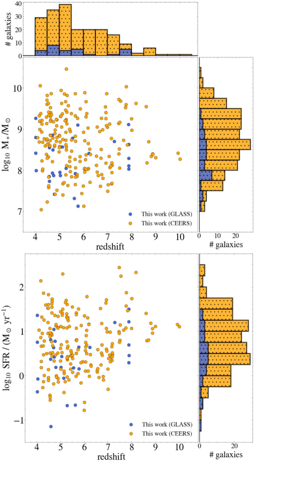
Figure 1: Figure showing the redshift distribution of stellar masses (top panel) and SFRs (bottom panel) for the galaxies selected in this paper. We highlight the redshift histogram of the entire sample on top of the first diagram, while the $M_{\star}\$and SFRs histograms are added on the right part of each panel. Galaxies coming from the CEERS and GLASS surveys are differentiated with a yellow and blue color, respectively.

We first consider spectra acquired through NIRSpec MSA observations by the GLASS-JWST ERS Program (PID 1324, PI: Treu; Treu et al. 2022) and by a JWST DDT program (PID 2756, PI: W. Chen; Roberts-Borsani et al. 2022). Both of them targeted galaxies residing over the central regions of the Frontier Field galaxy cluster Abell 2744. However, they were obtained using two different setups and different exposure times. The former were taken in high-resolution grating mode with three spectral configurations (G140H/F100LP, G235H/F170LP, and G395H/F290LP), covering a wavelength range from $1.5$ to $5.14\mu m$ at R $\sim 2000$-$3000$, and with a total integration time (per grating) of 4.9 hours. The latter instead were taken in low-resolution mode with the CLEAR filter + prism configuration, which provides a continuous wavelength coverage from $0.6$ to $5.3\mu m$ at R $\sim 30$-$300$. The prism resolution in the red part of the spectrum is enough to resolve and detect redshifted rest-frame optical emission lines, such as H$\beta$  and [O iii] $\lambda 5007\AA$. The exposure time in this case is of $1.23$ hours. The details of the spectral reduction, wavelength and flux calibration are described in detail in Mascia et al. (in prep.). Since GLASS-JWST observations target sources behind a lensing cluster, we adopt the global properties presented in Mascia et al. (2023), who correct stellar masses, line fluxes, SFRs, and galaxy sizes for magnification effects using the latest lensing model of Bergamini et al. (2023).

We also consider the spectra obtained by the CEERS survey through the NIRSpec MSA mode. The CEERS spectroscopic data were acquired over $3$ different observing epochs and in $8$ different pointings. The NIRSpec pointings named p4, p5, p7, p8, p9, and p10 were observed with the three NIRSpec medium resolution (G140M, G235M, and G395M) gratings, covering the rest-frame wavelength range $0.97$-$5.10\mu m$ with a resolving power R $\sim 1000$. In addition, p4, p5, p8, p9, p11, and p12 were also observed with the low resolution prism. In all cases, the exposure time is of $3107$s per spectrum. Three-shutter slitlets with a three-point nodding pattern were also used to enable accurate background subtraction. After the observing run, some galaxies have spectra obtained with both the prism and M-grating configuration, in which case we prioritize the latter, as the higher resolution of the M-grating improves the detection of faint emission lines with low S/N. The main steps of the reduction, the optimal extraction of the final 1D spectra, including also the wavelength and flux calibration, follow those described in other works of our collaboration, namely Fujimoto et al. (2023), Kocevski et al. (2023), and Arrabal Haro et al. (2023). A more detailed description of the NIRSpec data processing and a final spectroscopic catalog of the entire survey will also be presented in Arrabal Haro et al. (2024, in preparation).

To build a sample of high redshift galaxies for our analysis, we visually checked all the 1D spectra provided by the above surveys in order to assign a first value to the spectroscopic redshift $z_{spec}$ based on the visual identification of relatively bright, optical emission lines, including [O ii] $\lambda 3727\AA$, H$\beta$, [O iii] $\lambda 5007\AA$, and H$\alpha$ . This process was guided by the previous knowledge of the photometric redshifts of all the sources, obtained with the code eazy (Brammer et al., 2008). In the next section, we will describe a more precise measurement of $z_{spec}$. We also remark that the spectroscopic redshifts were checked and confirmed independently by other team members in both the GLASS and CEERS collaborations. Part of our spectroscopic sample is already published by other works (e.g., Arrabal Haro et al., 2023; Mascia et al., 2023, 2024), in which case we just checked the consistency of our $z_{spec}$ measurements.

Among the sample observed with NIRSpec by either the GLASS or CEERS survey, we selected galaxies with a spectroscopic redshift $z_{spec}$ $\geq 4$. The reason of this lower limit is twofold. First, we aim at studying the properties of the galaxy population as we approach the epoch of reionization, where most of the scaling relations addressed in this work are still largely unexplored compared to Cosmic Noon ($1<z<3$). Secondly, targets with $z\geq 4$ were the main priority of the GLASS and CEERS spectroscopic surveys, thus we have better statistics in this range. This condition yields a final sample of $230$ galaxies that we consider in our analysis. Among this sample, $19$ have H-grating spectroscopic data (R$\sim 2700$) in GLASS, $93$ have M-grating spectroscopy from CEERS (R$\sim 1000$), while $15$ and $114$ are observed in prism configuration (R$\sim 100$) in the Abell 2744 and EGS fields, respectively. The global population spans a redshift range between $z=4$ and $10.4$, with a median value $z_{med}=5.4$ (see Fig. 1-top). The number of sources decreases toward higher redshifts, with $11$ selected galaxies residing at redshift $\geq 8$.

Given the variety of observational programs considered, it is useful to better investigate the properties of our selected sample to assess potential biases on our analysis. The GLASS observations with NIRSpec cover approximately $50$ arcmin² in the sky. Given the relatively long exposure times, they are among the deepest available so far, as we can detect emission lines with fluxes down to a few $10^{-18}$ erg/s/cm². In addition, the lensing magnification is ideal for improving the detection of the intrisically faint, low-mass galaxy population at the epoch of reionization. The primary science targets of the NIRSpec observations were placed into open Microshutters (MSA), and were chosen based on previous spectrophotometric catalogs available from the GLASS team and from the literature. Many of them already had a confirmed spectroscopic redshift, while the remaining systems were photometrically selected at $z>4$ using previous HST observations in the region of Abell 2744 (see Treu et al. 2022 for more details). The CEERS spectroscopic observations cover instead a larger area in the sky of about $90$ arcmin², but they are shallower compared to GLASS. Some of the spectroscopic targets are HST-selected in the UV rest-frame (among which we find those galaxies falling outside of the NIRCam coverage), while additional targets benefitted from NIRCam observations undertaken in the first observing run (prior to NIRSpec observations), and therefore are optically selected, even though they might still be biased to UV-bright LBG-type objects as they are chosen based on their photometric redshift. While a more detailed description will be included in Finkelstein et al. (2024, in prep.), we note that it is difficult to precisely assess the selection function even within the same survey. It is thus a better approach to analyze a posteriori the galaxy properties as a whole.

Even though GLASS probes slightly lower masses and SFRs on average compared to CEERS, the two subsets are similarly distributed in redshift, as shown in the top histogram of Fig. 1-top, and they are located along the same $M_{\star}\$vs SFR relation. Moreover, in the redshift evolution of $\Sigma_{\rm SFR}$, and in all the other diagrams analyzed in this paper, removing the small GLASS subset does not significantly change the results and the best-fit relations, meaning that they satisfy the same physical trends. We also note from Fig. 1 that both subsets may suffer from slight incompleteness at redshift $\geq 8$, where we may lose a fraction of galaxies at the lowest masses and SFRs (respectively $\log$ $M_{\star}\$/$M_{\odot}\$$<8$ and $\log$ SFR/(M_⊙/yr) $<0$. However, as will be shown later in Section 3.3, our galaxies can be fairly considered as representative of the star-forming ‘Main Sequence’ for most part of our redshift range.

Finally, even though the standard STScI reduction pipeline adopted for our spectra already includes a slit loss correction, we further checked the absolute flux calibration of the output 1D spectra by comparing them to the available broadband photometry (see Section 2.3 for the specific filters used). Despite the calibration corrections for individual photometric bands do not show a significant wavelength dependence, as also found by other works in the collaboration (e.g., Napolitano et al., 2024), we limit the comparison to the redder spectral range at $2\mu m<\lambda<5\mu m$, as the S/N of the continuum rapidly drops at lower wavelengths, making this check and comparison more difficult. A second reason for this choice is that we are interested only in optical rest-frame lines, which mostly lie in the red part of the spectrum. For the correction, we apply to the spectrum a constant multiplicative factor, which is obtained as the median value of the corrections derived independently for all the photometric bands whose central wavelengths reside in the above spectral range.

2.2 Line measurements and derivation of star-formation rates

We measure emission line properties with a similar methodology to that adopted in Calabrò et al. (2019) and Calabrò et al. (2023). In brief, we use a python version of the $\chi^{2}$ minimization routine mpfit (Markwardt, 2009) to fit the following, rest-frame optical, emission lines: [O ii] $\lambda 3727\AA$, H$\gamma$ , [O iii] $\lambda 5007\AA$, H$\beta$ , and H$\alpha$ , by assuming a common redshift and line velocity width $\sigma$, with a tolerance of $100$ ($1000$) km/s on the line centroid and $\sigma$ for the H- or M-grating and prism spectra, respectively. The fit of the emission lines yields the exact redshift of the sources, the line widths, the line fluxes, and their corresponding uncertainties. The quality of the fit is controlled through the reduced $\chi^{2}$ and visual inspection for each galaxy. We consider the lines as detected above a S/N of $3$, while, for non-detected lines, we adopt $3\sigma$ upper limits, which then are propagated into all the physical quantities derived. As discussed in Calabrò et al. (2023), the underlying stellar absorption for Balmer lines can be neglected as it does not produce significant variations of the emission line fluxes for galaxies in our stellar mass range. Moreover, our galaxies have typically younger ages, lower metallicity and lower dust content compared to the lower redshift CEERS sample analyzed in Calabrò et al. (2023), therefore the underlying absorption is expected to be even smaller (Groves et al., 2012). For this reason, we do not correct the emission line fluxes for stellar absorption. We also notice that in low resolution spectra acquired with the prism configuration, H$\alpha$ is blended with the [NII] doublet. However, our galaxies are all very low-mass and with sub-solar metallicities, for which the expected contamination is less than $10\%$, according to lower redshift studies (Faisst et al., 2018). A negligible contribution of [N ii] to H$\alpha$ for galaxies at $z>4$ is also found by the photoionization models described in Simmonds et al. (2023), and supported by the results from our high resolution dataset. As a consequence, we do not attempt to make any correction on the H$\alpha$ flux in prism spectra. Finally, two sources at redshifts $5<z<6$ with clear broad H$\alpha$  components and narrow [O iii] $\lambda 5007\AA$, indicative of broad-line AGN emission, are removed from the sample. We refer to Calabrò et al. (2023) for a more detailed discussion of the emission line measurement.

As a first step of our analysis, we compute the gas-phase attenuation A_V from the available Balmer lines (among H$\gamma$ , H$\beta$, and H$\alpha$ ) assuming a dust-screen, Milky Way like extinction law (Cardelli et al., 1989). If only one Balmer line is detected, we adopt an A_V as inferred from the SED fitting procedure described later in Section 2.3. As shown in the Appendix of Calabrò et al. (2023), hydrogen recombination lines across a large range of wavelengths ($\sim 0.4$ to $\sim 2\mu m$) are overall in agreement with the predictions of typical dust attenuation models, even when the lines reside in different gratings, indicating that their relative calibration and the inferred values of A_V are generally reliable. From the fluxes of the [O ii] $\lambda 3727\AA$ and [O iii] $\lambda 5007\AA$ lines, we also derive the O32 index, defined as the logarithm of the reddening corrected [O iii] $\lambda 5007\AA$/[O ii] $\lambda 3727\AA$ ratio.

We then derive the star formation rates as follows. We first compute the observed, dust-corrected H$\alpha$ luminosity L_Hα. If H$\alpha$ is not detected, we consider the fluxes of H$\beta$ (or H$\gamma$ as last possibility), corrected for dust attenuation and rescaled to H$\alpha$ assuming the intrinsic ratios of $2.86$ and $6.10$ (respectively for H$\beta$ and H$\gamma$ ), valid for case B recombination, for a temperature $T=10000$K, and an electron density $n_{e}=10^{2}$ cm^-3 (Osterbrock, 1989). We then convert L_Hα to SFR assuming the calibration of Reddy et al. (2022) as SFR $=$ L_Hα $\times$ $10^{-41.67}$. This is the most suited calibration according to the typical subsolar metallicities expected for our galaxies at $z>4$, and reflects the greater efficiency of ionizing photon production in metal poor stellar populations. In our sample, we obtain the SFR from H$\alpha$ in $153$ galaxies, from H$\beta$ in $67$ systems, while for $10$ galaxies it is inferred from H$\gamma$ . The resulting SFR distribution is shown in Fig. 1-bottom: our galaxies span values between $\sim 0.1$ and $300$ $M_{\odot}\$/yr, with a median SFR of $\sim 5$ $M_{\odot}\$/yr.

We note possible caveats of our analysis, affecting the relation between the SFR and H$\alpha$ luminosity. For example, the diffuse warm ionized gas (DIG) or collisional excitation in the ISM might contribute to the observed H$\alpha$ emission, leading us to slightly overestimate the SFRs. On the other hand, part of the ionizing radiation may be absorbed by dust and helium, or might escape from the galaxy, reducing the amount of Lyman continuum (LyC) photons available for hydrogen line emission. This might lead us to slightly underestimate the total SFR of the galaxy. Modeling and testing these effects is difficult, especially at high redshift. However, despite these uncertainties, the simple analysis performed in this paper and the dust correction through the Balmer decrement should work well as a first approximation, as shown by Tacchella et al. (2022).

We also note that the dust correction is another potential source of uncertainty. This is due both to a poor theoretical understanding of dust production mechanisms and dust growth in the ISM at high redshift (see discussion in Markov et al. 2023), and to the lack of observational constraints. For this reason, different dust attenuation and extinction laws measured in the local Universe are usually adopted in the literature also at early epochs. We remark that our choice for dust correction is the same adopted by similar works on NIRSpec galaxies at the epoch of reionization (e.g., Llerena et al. 2024, in prep.). Adopting a Calzetti et al. (2000) attenuation law, as done for example in Mascia et al. (2024), does not significantly alter the results.

2.3 Photometric data and estimation of stellar masses through SED fitting

We derive stellar masses for our galaxies through an SED fitting procedure using the code cigale (Boquien et al., 2019), version 2022.1. We fit Bruzual & Charlot (2003) stellar population models with Chabrier IMF to the available observed photometry ranging from $0.5$ to $8\mu m$. There is a homogeneous photometric coverage for all the galaxies in our sample. In particular, all the galaxies observed by the GLASS survey are covered by JWST/NIRCam imaging from the UNCOVER program (JWST-GO-2561; Bezanson et al. 2022). For this subset, fluxes and uncertainties are obtained in the F115W, F150W, F200W, F277W, F356W, F410M, and F444W filters, using the catalog of Paris et al. (2023). The majority of our NIRSpec sources in the EGS field are also covered by JWST/NIRCam observations from the CEERS survey in the same filters listed above (Bagley et al., 2023). For this subset, we take the photometric fluxes and uncertainties from Finkelstein et al. (2023). However, a subset of CEERS sources ($79$) do not have JWST imaging. To ensure also in this case a complete coverage of the UV and optical rest-frame emission for the SED fitting, we consider the following broadband filters: HST/ACS F606W and F814W, HST/WFC3 F125W, F140W, and F160W, CFHT/WIRCAM J, H, and K_s, Spitzer IRAC 3.6 and 4.5 $\mu m$. In particular, we use the photometric fluxes and associated uncertainties from the multi-wavelength catalog assembled by Stefanon et al. (2017).

The SED fitting with cigale is performed as follows. We consider a main stellar population with metallicities Z${}_{\ast}=0.0004$, $0.004$, $0.008$, or $0.02$, and a delayed SFH parameterized by an e-folding time that can assume the following values: $10$, $100$, $500$, and $1000$ Myr, and with a grid of $18$ possible stellar ages ranging from $50$ Myr to $1.3$ Gyr. We also include the possibility of a recent exponential burst with SFH $\propto\exp^{-t/\tau_{burst}}$, where $\tau$ can assume the values $1$, $20$, and $50$ Myr, while the ages can range from $5$ to $50$ Myr. We also allow the mass fraction of the late burst population to vary from $0$ to $80\%$ of the total mass formed in the entire galaxy history. We include contribution from nebular emission, where the nebular component is parametrized with an electron density $n_{e}$ of $100$ cm^-3, subsolar gas-phase metallicity equal to the stellar metallicity, and ionization parameter between $-3$ and $-2$. Finally, dust attenuation of the stellar and nebular components are modeled with a Milky Way extinction curve (Cardelli et al., 1989), and parametrized with a color excess E(B-V)_stellar ranging from $0$ to $3$ in steps of $0.05$, a total to selective extinction R${}_{V}=3.1$, and a stellar continuum to nebular attenuation ratio of $0.44$ (Calzetti, 2001). Therefore, for each galaxy, an A_V is computed as R_V $\times$ E(B-V). The intergalactic medium (IGM) transmission is also taken into account following the model of Meiksin (2006).

We find stellar masses $M_{\star}\$ranging from $10^{7}$ to $10^{10.5}$ $M_{\odot}\$(see Fig. 1-top), with a nearly symmetric distribution around a median $\log_{10}$ $M_{\star}\$/$M_{\odot}\$$=8.7$ ($1\sigma=0.7$). Combining these results with the SFR measurements described in the previous section, we find that the bulk of our galaxy population has sSFRs between $1$ and $100$ Gyr^-1, with median value of $10$ Gyr^-1. For galaxies fitted with E(B-V)$=0$, we also set an upper limit on their dust attenuation as E(B-V)$=0.05$, corresponding to our grid step and to the average uncertainties obtained with this methodology. Comparing the values of A_V,nebular obtained from the SED fitting to those estimated from Balmer lines, we find that they are overall consistent with the $1:1$ relation, even though with a large scatter.

For galaxies with multiple coverage, we have also checked that removing NIRCam photometry and using only the remaining bands (HST + Spitzer + ground) in the SED fitting yields $M_{\star}\$that are in agreement with estimates based on JWST photometry in the entire range spanned by our sample. Therefore, we do not introduce systematic biases (related to the measurement method) on the derived parameters for the subset that is not covered by JWST imaging. Finally, our stellar masses are consistent with those obtained using the code zphot (Fontana et al., 2000) with a similar setup and SFH to our cigale run, indicating that this quantity is rather robust and not significantly affected by the exact fitting procedure.

2.4 Galaxy sizes and SFR surface density estimation

We measure the major-axis half-light radius $r_{e}$ of our galaxies by fitting with the python software galight (Ding et al., 2021) their rest-frame UV images, because we want to primarily trace star-formation from the emission of young massive stars. A subset of $151$ galaxies is covered by JWST imaging, in which case we adopted the background-subtracted mosaics described in Bagley et al. (2023) and Paris et al. (2023), for the CEERS and GLASS subset, respectively. For the remaining subset of $79$ galaxies (all in the CEERS field), we use instead HST imaging (Koekemoer et al., 2011). Since we are interested in the extension of recent star-formation (i.e., of young and massive stars), to homogeneously probe the same rest-frame UV window, we performed the measurements in the F115W band for galaxies at $z<5.5$, in the F150W filter for those at slightly higher redshifts ($5.5<z<7.5$), and in F200W for systems at $z>7.5$. In cases where only HST imaging is available, we adopted the F125W and F160W band for galaxies at redshifts lower and higher than $5.5$, respectively.

In detail, we first produce cutouts with size $3\arcsec\times 3\arcsec$, which are given as input to the galight code. All sources in the cutout, including the central galaxy of interest, are fitted simultaneously assuming that they are well represented by a Sersic profile. We constrain the following parameters to keep the fit within physically meaningful values: the Sersic index is free to vary from $0.2$ to $8.0$, and the axis ratio $q$ is set in the range $0.1<q<1$. After running galight, sources are flagged according to the quality of the fit, with a flag $=0$ assigned to reliable fits, and flag $=1$ for sources that are not fitted well by the above procedure (indicative of a more complex shape), as checked visually in the observed vs best-fit luminosity profile that is output by the code. As a result, $213$ galaxies with a good size quality flag are considered when analyzing the $\Sigma_{\rm SFR}\$in the following sections.

The size uncertainties are assessed in accordance with Yang et al. (2022) and rescaled based on the signal-to-noise ratio derived from the photometry. Previous studies (e.g., Kawinwanichakij et al., 2021) have shown that the outcomes from galight are robust, and consistent with estimations made through conventional softwares like Galfit (Peng et al., 2002). A subset of our galaxies are indistinguishable from point sources. In particular, we performed a subset of simulations, finding that $0.025\arcsec$ and $0.1\arcsec$ are the smallest measurable sizes in JWST and HST images, respectively. Therefore, we set these values as upper limits. In our sample, $64$ galaxies of $213$ ($\sim 30\%$) are unresolved and have upper limits on $r_{e}$. We also notice that for the galaxies lying in the GLASS field (which are all covered by JWST imaging), we directly adopt the measurements already performed by Mascia et al. (2023), following a similar methodology based on the galight software and corrected for the effect of lensing magnification.

With the estimated sizes, we compute the galaxy-integrated SFR surface densities for all the objects. A subset of $25$ extremely compact galaxies have an upper limit on the size but also an upper limit on the SFR. We exclude these galaxies from the analysis as their $\Sigma_{\rm SFR}\$would be totally unconstrained. As a result, the investigation of the redshift evolution of $\Sigma_{\rm SFR}\$and its dependence on other galaxy properties will be made on a sample of $188$ galaxies. The distribution of $\Sigma_{\rm SFR}$ for this galaxy subset has a median value of $\log_{10}\Sigma_{\rm SFR}=0.6$ (in units of $M_{\star}\$/yr/kpc², $1\sigma=0.8$), with individual systems spanning the logarithmic range between $-1.5$ and $2.5$.

3 Results

We explore in this section the redshift evolution of $\Sigma_{\rm SFR}\$for our selected sample, and then focus on fundamental scaling relations involving $M_{\star}\$, SFR, and $\Sigma_{\rm SFR}\$in the entire redshift range between $\sim 4$ and $\sim 10$. To characterize all the 2D distributions presented in this paper and quantify the level of correlation between two quantities, we adopt two different approaches throughout this work, both of which take into account (in a different way) the presence of upper and lower limits in the data. We explain them in detail in the next subsection for the redshift vs $\Sigma_{\rm SFR}\$diagram, but the same steps of the analysis are followed for the other diagrams.

3.1 Fitting methods

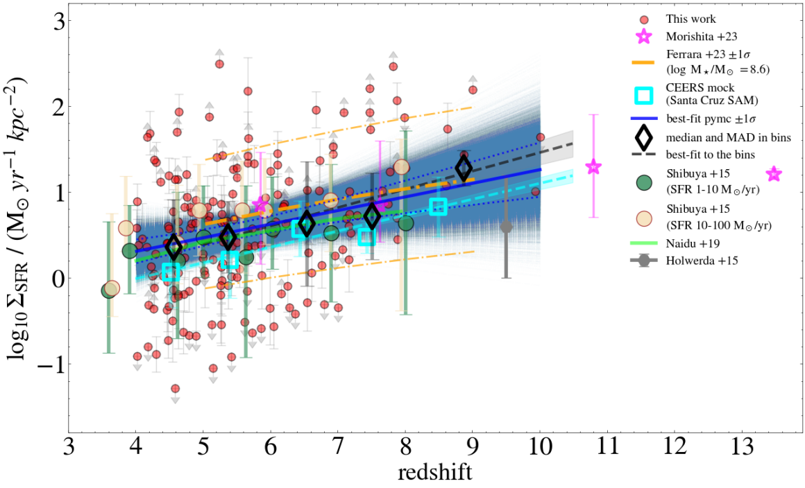
Figure 2: Redshift evolution of $\Sigma_{\rm SFR}\$from $z=4$ to $10$. The median values and MAD of $\Sigma_{\rm SFR}\$in bins of increasing redshift are shown with black empty diamonds and black vertical error bars, while the best-fit to the bins is represented with a black dashed line with a gray region indicating its $1\sigma$ uncertainty. The best-fit obtained with the Bayesian linear regression is shown with a blue continuous line, with the blue dotted lines and the blue shaded regions representing the $1\sigma$ uncertainty and the ´posterior plot’, respectively. Theoretical model predictions and comparison observations are included as specified in the legend.

x	y	redshift range	best-fit bins	best-fit pymc
$z$	$\log$ $\Sigma_{SFR}$/($M_{\odot}\$/yr/kpc2)	all	$m=0.21\pm 0.03$     $q=-0.7\pm 0.2$	$m=0.16\pm 0.06$     $q=-0.3\pm 0.4$
$\log$ M⋆/$M_{\odot}\$	$\log$ SFR/($M_{\odot}\$/yr)	low-z	$m=0.68\pm 0.07$     $q=-5.3\pm 0.6$	$m=0.7\pm 0.06$     $q=-5.5\pm 0.5$
$\log$ M⋆/$M_{\odot}\$	$\log$ SFR/($M_{\odot}\$/yr)	high-z	$m=0.55\pm 0.12$     $q=-4.0\pm 1$	$m=0.76\pm 0.07$     $q=-6\pm 0.6$
$\log$ M⋆/$M_{\odot}\$	$\log$ $\Sigma_{SFR}$/($M_{\odot}\$/yr/kpc2)	low-z	$m=0.16\pm 0.10$     $q=-1.0\pm 0.9$	$m=0.19\pm 0.09$     $q=-1.1\pm 0.7$
$\log$ M⋆/$M_{\odot}\$	$\log$ $\Sigma_{SFR}$/($M_{\odot}\$/yr/kpc2)	high-z	$m=0.4\pm 0.2$      $q=-3\pm 2$	$m=0.30\pm 0.15$     $q=-1.7\pm 0.9$

Table 1: Table with the best-fit linear relations of the diagrams analyzed in this work. The first two columns indicate the $x$ and $y$ axis quantities, while the last two columns highlight the best fit coefficients of the linear relations ($y=m\times x+q$) obtained with two different approaches, as described in the text. The third column indicates whether the relation is derived with the subset at lower redshift ($4<z<6$), at higher redshift ($6<z<10$), or in the entire $z$ range.

As a first approach to characterize the redshift evolution of $\Sigma_{\rm SFR}\$, we compute the median redshift and the median $\Sigma_{\rm SFR}\$of galaxies falling in different, well defined bins of increasing spectroscopic redshift ($4$-$5$, $5$-$6$, $6$-$7$, $7$-$8$, $>8$), which are shown as black empty diamonds in Fig. 2. In each bin, we also calculate the median absolute deviation (MAD) of $\Sigma_{\rm SFR}\$, which is indicated with black error bars. In this calculation, we assign half of the $\Sigma_{\rm SFR}\$value to galaxies with $3\sigma$ upper limits, or twice the value in case of $3\sigma$ lower limit on $\Sigma_{\rm SFR}\$. Then, we derive a global, best-fit linear relation and $1\sigma$ limits through Monte Carlo simulations. In detail, we perform $1000$ realizations of our data varying the data points according to their x and y axis $1\sigma$ uncertainties. For each realization, we repeat the same process of median $\Sigma_{\rm SFR}\$estimation in each of the previously defined redshift bins, and fit these median values with a first order polynomial. We finally derive the best-fit relation as the median slope and normalization of all the different realizations, including the uncertainties as their standard deviation.

In the second analysis method, we use the Python package PyMC https://doi.org/10.5281/zenodo.10371446 . This is an advanced tool for statistical modeling featuring next-generation Markov chain Monte Carlo (MCMC) sampling algorithms such as the No-U-Turn Sampler (NUTS; Hoffman et al. 2014), a self-tuning variant of Hamiltonian Monte Carlo (HMC; Duane et al. 1987). HMC and NUTS can manage complex posterior distributions and fitting models, taking advantage of gradient information from the likelihood to achieve much faster convergence than traditional sampling methods. A first advantage of this approach is that it can be applied to the entire dataset without dividing the sample in multiple bins as in the previous case. A second advantage is that it implements the methods of the Bayesian survival analysis in the linear regression to deal with upper and lower limits on the y axis. Most importantly, this method does not impute the limits (i.e., does not strictly substitute them with a different value), but instead integrates them out through the likelihood. In pratice, the entire dataset is fitted with a linear relation, obtaining a first guess of the line parameters. Then, pyMC is run by assuming Gaussian priors for the slope and intercept, with $\sigma=1$ and the first guesses as centers. At this step, normal measurements, upper and lower limits are considered simultaneously in the fit. Finally, the full posterior distributions of the slope and intercept are used to calculate the mean linear relation, the $1\sigma$ uncertainty, and for showing the ´posterior plot’, that is, a stack of random draws from the posterior distribution of the slope and intercept. We report in Table 1 the best-fit parameters obtained for the main relations studied in this paper and using both the linear regression methods described above.

3.2 The redshift evolution of the SFR surface density

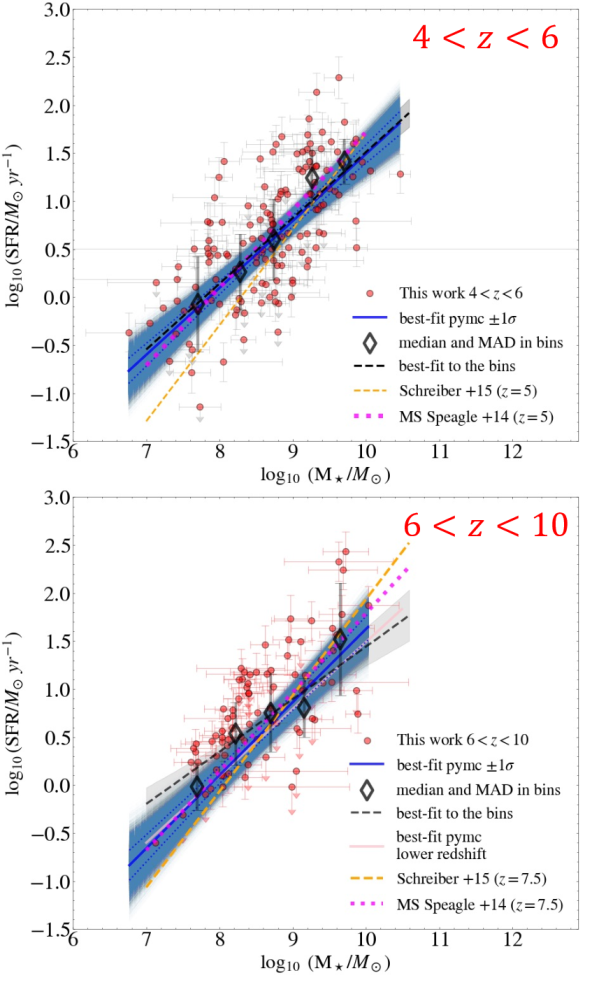
Figure 3: Top: Diagram showing the star-forming ‘Main Sequence’ of galaxies selected in this work in the redshift range $4<z<6$. For comparison, the high redshift and low-mass extrapolation of the MS relations by Schreiber et al. (2015) and Speagle et al. (2014) (obtained at lower redshifts and higher $M_{\star}\$) are shown with dashed orange and dotted fuchsia lines, respectively. Bottom: Same as above, but for the redshift range $6<z<10$. The Bayesian best-fit relation obtained in the lower redshift bin in included as a pink continuous line for comparison.

Our results for the evolution of $\Sigma_{\rm SFR}\$are shown globally in Fig. 2, where the median $\Sigma_{\rm SFR}\$and MAD in five increasing bins of redshift (defined as $4$-$5$, $5$-$6$, $6$-$7$, $7$-$8$, and $>8$) are represented with empty diamonds and vertical error bars, while the best-fit to the bins is highlighted with a black dashed line and a gray shaded area indicating its $1\sigma$ uncertainty. In addition, we also consider the Bayesian fitting method, plotting the mean linear relation as a blue continuous line, the $1\sigma$ uncertainty as blue dotted lines, and the ´posterior plot’ as a blue shaded region around the mean relation.

Regardless of the analysis approach, we find a mild evolution of $\Sigma_{\rm SFR}\$from $z\simeq 4$ to $z\sim 8$, with a slight but statistically significant increase by a factor of two ($0.3$ dex), going from $2.5$ $M_{\odot}\$/yr/kpc² to $\sim 5$ $M_{\odot}\$/yr/kpc². We note that in the short cosmic epoch that we are exploring ($\sim 1$ Billion years of cosmic history), the linear relation yields a good description of the increase in $\Sigma_{\rm SFR}\$. In all cases we obtain a positive correlation with best-fit slopes of $0.16\pm 0.06$ and $0.21\pm 0.03$, respectively from the Bayesian regression and the fit to the bins. Therefore, in all cases we can exclude a flat trend at least at $2\sigma$ level.

Fitting the median $\Sigma_{\rm SFR}\$in the five redshift bins, the slope is slightly higher compared to the other method, the reason being a sudden rise of the $\Sigma_{\rm SFR}\$in the last bin at $8<z<10$, where we reach a median $\Sigma_{\rm SFR}\$of $\sim 20$ $M_{\odot}\$/yr/kpc². However, we notice that the median $\Sigma_{\rm SFR}\$derived in the last bin is consistent with the Bayesian fit within $1\sigma$, and with the linear fit to only the four lower redshift bins within $2\sigma$. Therefore, the upturn of $\Sigma_{\rm SFR}\$at $z>8$ is not significant from our data: the trend in the last bin may simply be driven by a poor statistics and may be also affected by the sample incompleteness discussed in Section 2.1. Moreover, we also anticipate that the semi-analytic models that we analyze in this paper predict a smoothly increasing linear trend of $\Sigma_{\rm SFR}\$out to $z=10$.

Both the normalization and the slope of our $\Sigma_{\rm SFR}\$- redshift relation are consistent with most of the previous observations. In particular, our Bayesian best-fit line falls exactly between the observed median relations estimated by Shibuya et al. (2015) up to redshift $8$ in two different bins of SFR ($1<$ SFR/$M_{\odot}\$/yr $<10$ and $10<$ SFR/$M_{\odot}\$/yr $<100$). Compared to these results, our findings indicate that the increase of $\Sigma_{SFR}$ can be extended up to at least redshift $10$. The median $\Sigma_{\rm SFR}\$between redshift $4$ and $9$ are overall consistent with those calculated by Morishita et al. (2023) with a sample similar to our study in terms of stellar masses and SFRs probed (fuchsia empty stars in Fig. 2). Moreover, NIRSpec galaxies ranging $8<z<10$ have $\Sigma_{\rm SFR}\$comparable to those recently derived in photometrically selected systems observed by JADES at much higher redshifts ($10$-$13$) by Robertson et al. (2023). Finally, our results are slightly higher, but still marginally consistent, than the range of $\Sigma_{\rm SFR}\$($1$-$20$ $M_{\odot}\$/yr/kpc²) measured by Holwerda et al. (2015) for $6$ galaxies at redshifts $9<z<10$ identified with HST in the CANDELS survey, even though these are intrinsically brighter systems compared to those analyzed in this work.

3.3 The main sequence of star-formation at $z>4$

We now focus on fundamental scaling relations describing the evolution of the galaxy population. The most important is that involving the star-formation rate and the stellar mass, which show a tight correlation at all redshifts, known as the star-forming ‘Main Sequence’ (SFMS, Noeske et al. 2007, Daddi et al. 2007, Santini et al. 2017). This relation is fundamental to understand the process of gas conversion into stars and subsequent build-up of stellar mass across cosmic time. While the slope is relatively constant with redshift, ranging from $\sim 0.6$ to $\sim 1$, depending on the sample selection and specific tracer used for the SFR, all studies agree that the normalization increases monotonically from lower to higher redshift up to at least $z\sim 7$.

In Fig. 3, we show the $M_{\star}\$vs SFR diagram for our selected spectroscopic sample. In order to check and better appreciate variations with redshift, we divide the sample in two redshift bins, that is, $4<z<6$ and $6<z<10$ (top and bottom panels, respectively). In both cases, we further divide the sample in different bins of stellar masses from $10^{7}$ to $10^{10.5}$ $M_{\odot}\$in steps of $0.5$ dex when performing the first approach of the analysis explained in Section 3.1. With all the fitting methods, we find in both redshift ranges a tight and significant correlation between $M_{\star}\$and the SFR, indicating that the SFMS is in place up to the highest redshifts ($z\sim 10$) explored by this work. Adopting the Bayesian regression as the reference method, the SFMS in the two redshift bins have similar slopes ($0.7\pm 0.06$ at $z<6$ and $0.76\pm 0.08$ at $z>6$), and the normalization of the relation is not significantly different between the two redshift bins in the $M_{\star}\$range from $=10^{7}$ to $=10^{10.5}$ $M_{\odot}\$.

Both the slope and normalization of our relations are generally in agreement with the extrapolations at redshift $5$ and $7.5$ (and down to a stellar mass of $10^{7}$ $M_{\odot}\$) of the SFMS relations derived for more massive and lower redshift star-forming galaxies by Speagle et al. (2014) and Schreiber et al. (2015), with a slightly better consistency with the shallower slope found by Speagle et al. (2014). We note that the evolution of SFR at fixed stellar mass expected in this redshift range ($\sim 0.15$ dex) is smaller than the scatter of the relation and too small to be appreciated with our dataset, given the uncertainties obtained in the fit. Our relations (both the slope and normalization) are also consistent with those recently found in CEERS by Cole et al. (2024) using photometrically selected galaxies at redshifts from $4.5$ to $12$, and $10$Myr-averaged SFRs estimated through SED fitting (see their Fig.7). This indicates that the spectroscopic selection is not significantly biased compared to a pure photometrical selection. These results also suggest that, even though our sample may suffer from incompleteness at $z\geq 8$ at the lowest masses and SFRs, this effect should not be large.

3.4 The main sequence of SFR surface density

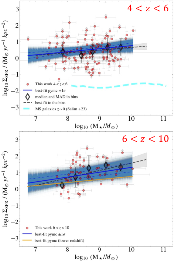
Figure 4: Figure showing the $\Sigma_{\rm SFR}\$ ‘Main Sequence’ for our selected galaxies in the lower redshift bin ($4<z<6$, top panel) and higher redshift bin ($6<z<10$, bottom panel). The lines, shaded areas, and markers are the same as in Fig. 2. The average location of massive ($M_{\star}\$$>10^{9}$ $M_{\odot}\$) star-forming galaxies at redshift $\sim 0$ presented by Salim et al. (2023) is highlighted with a cyan dashed line.

The galaxy integrated $\Sigma_{\rm SFR}\$has been proposed as an alternative and more physical measurement of the current SF activity of galaxies, the reason being a closer connection to the gas density and the efficiency of stellar feedback compared to the specific SFR. For example, the incidence of outflows has been shown to correlate better with the $\Sigma_{\rm SFR}\$ rather than with the offset from the standard SFMS (Förster Schreiber et al., 2019). Moreover, $\Sigma_{\rm SFR}\$ also incorporates, by construction, information about the galaxy structure and morphology. For this reason, an alternative ‘Main Sequence’ relation has been defined as the main locus occupied by star-forming galaxies in the $\Sigma_{\rm SFR}\$- $M_{\star}\$plane. Compared to the sSFR, the $\Sigma_{\rm SFR}\$ properties of galaxies are more uniform at varying stellar masses, such that $\Sigma_{\rm SFR}\$ is approximately constant across the Main Sequence, as found by Schiminovich et al. (2007) and Salim et al. (2023) for relatively low redshift galaxies ($z\lesssim 1$). However, there could also be deviations from this flat relation, indicating additional (or lower) star-formation activity associated with different galaxy structures. For example, moderately positive correlations between $\Sigma_{\rm SFR}\$and $M_{\star}\$are observed at $M_{\star}\$$>10^{9}$ $M_{\odot}\$by Salim et al. (2023) for star-forming galaxies from $z=0$ to $z=2$, which are interpreted as the build-up of a central bulge component in those galaxies.

We now explore the $\Sigma_{\rm SFR}\$ vs $M_{\star}\$ diagram for the NIRSpec galaxies, divided in two redshift bins ($4<z<6$ and $6<z<10$), as done for the classical SFMS. Our results are shown in Fig. 4. We find that in both redshift bins there is a very mild correlation, with $\Sigma_{\rm SFR}\$slightly increasing in more massive galaxies: the best-fit slopes obtained with the Bayesian regression method are of $0.19\pm 0.09$ and $0.30\pm 0.15$, respectively in the low and high redshift bins. This tells us that the data points are still consistent (within $3\sigma$) with a constant $\Sigma_{\rm SFR}\$as a function of $M_{\star}\$in the entire redshift of our work. Considering the large range spanned by $\Sigma_{\rm SFR}\$(by more than three orders of magnitude), it is indeed remarkable to observe a median variation of only less than $0.5$ dex across more than $\sim 3$ orders of magnitude of stellar mass, from $\log$ $M_{\star}\$$=7$ to $\sim 10$. For the higher redshift sample we also find a slightly higher normalization of the $\Sigma_{\rm SFR}\$-‘Main Sequence’ by $\sim 0.5$ dex (at $M_{\star}\$$=10^{9}$ $M_{\odot}\$) compared to the subset at $z<6$.

The very mild increase of $\Sigma_{\rm SFR}\$with $M_{\star}\$is in agreement with previous observations of star-forming galaxies at comparable masses but at lower redshifts (Förster Schreiber et al., 2019; Schiminovich et al., 2007; Salim et al., 2023). In such comparisons, we do not find clear evidence of a sudden or significant upturn of the relation in the entire mass range that we explore. However, the normalization of the $\Sigma_{\rm SFR}\$-‘Main Sequence’ is significantly higher compared to lower redshift studies. The median $\Sigma_{\rm SFR}\$of our galaxies at $z\sim 5$ is of $\sim 2.5$ $M_{\odot}\$/yr/kpc² ($\log$ $\Sigma_{\rm SFR}\$$=0.4$). At fixed stellar mass, and focusing on the overlapping stellar mass region ($8<\log$ $M_{\star}\$/$M_{\odot}\$$<10$), our $\Sigma_{\rm SFR}\$values are higher compared to the local Universe by approximately $2$ dex at $z\sim 5$ and $2.5$ dex at $z\sim 10$, indicating a strong evolution of $\Sigma_{\rm SFR}\$with cosmic time.

4 Discussion

In this section we further analyze our results to better understand how the fundamental quantity $\Sigma_{\rm SFR}\$is related to other phsyical properties of the galaxies during and immediately after the epoch of reionization.

4.1 Comparison to predictions of theoretical models

We compare our observations to some theoretical models that have been introduced to explain galaxy evolution across cosmic epochs. Focusing on the redshift evolution of $\Sigma_{\rm SFR}\$, we first consider the empirical model of Naidu et al. (2020). As already mentioned in Section 1, the main assumption of this model is that $f_{esc}\$is solely dependent on $\Sigma_{\rm SFR}\$as $f_{esc}\$$=$ a $\times$ $\Sigma^{b}_{\rm SFR}$, with $a=1.6\pm 0.3$ and $b=0.4\pm 0.1$. As shown in Fig. 2, this model yields an evolution of $\Sigma_{\rm SFR}\$up to redshift $\sim 8$ (lime curve) that is fully in agreement with our best-fit relation.

As an additional test, we compare our observations to the physical model presented by Ferrara et al. (2023) and Ferrara (2024). In detail, we take the redshift evolution of the SFR predicted by their model, and derive the $\Sigma_{\rm SFR}\$by combining it with the empirical size evolution found by Morishita et al. (2023). At the median stellar mass of the sample plotted in Fig. 2 ($\log$ $M_{\star}\$/$M_{\odot}\$$=8.6$), we obtain a slightly increasing trend of $\Sigma_{\rm SFR}\$, highlighted with a dash-dotted orange line, whose slope is remarkably consistent with our data and with the model of Naidu et al. (2020). Even though is has a slightly higher normalization of $\sim+0.2$ dex, this is well below the uncertainties of our best-fit relation. We note that the prediction is very sensitive not only to the stellar mass considered (lower $M_{\star}\$have systematically lower $\Sigma_{\rm SFR}\$), but especially to the effective radius. Indeed, considering the uncertainties on the best-fit redshift-size relation of Morishita et al. (2023), we would obtain an uncertainty on the normalization of the predicted $\Sigma_{\rm SFR}\$evolution of $\sim 0.8$ dex, higher than the median absolute deviation (MAD) of our sample.

Finally, we also take the CEERS mock galaxy catalog (Yung et al., 2022) for comparison. This catalog covers an area overlapping with the observed EGS field, and contains galaxies over $0<z\lesssim 10$. The galaxies in the mock lightcone are simulated with the Santa Cruz SAM for galaxy formation (Somerville & Davé, 2015; Somerville et al., 2021). The free parameters in the model are calibrated to reproduce a set of galaxy properties observed at $z\sim 0$ and have been shown to well-reproduce the observed evolution in high-redshift ($z\gtrsim 4$) one-point distribution functions of $M_{\rm UV}$, $M_{\ast}$, and SFR (Yung et al., 2019a, b). The effective radii of these simulated galaxies are determined as described in Brennan et al. (2015) and are shown to be in good agreement with CEERS observations at $3<z<6$ (Kartaltepe et al., 2023).

From the mock lightcone, we extract a random sample of galaxies that has a redshift and a stellar mass distribution similar to our observed sample, and then apply a magnitude cut as F277W $<29.15$ to match the depth of the CEERS survey (Finkelstein et al., 2023), where most of our galaxies come from. With this selection method, fitting the median $\Sigma_{\rm SFR}\$in five bins of redshift as done for the real data, we obtain an increasing trend of $\Sigma_{\rm SFR}\$with redshift that is very similar to the observational result. In addition, the SAM best-fit relation has a slightly lower normalization than the observed one by $\sim 0.2$ dex. As in the previous case, this is due to predictions on galaxy sizes, which are slightly larger on average compared to our values and to the size evolution obtained by Morishita et al. (2023). Despite this, the difference in $\Sigma_{\rm SFR}\$normalization is rather small and below the $1\sigma$ uncertainties. Therefore, the SCSAM yields a good representation of the observed properties of galaxies in the entire redshift range from $4$ to $\sim 10$. A similar good consistency between SCSAM model predictions and observations is obtained also for all the other diagrams studied in Section 3 and in Section 4. The models analyzed in this section also agree on the strong evolution of $\Sigma_{\rm SFR}\$from $z=0$ to the reionization epoch mentioned in Section 3.4. To conclude, our results are consistent not only with previous observations, but also with a variety of theoretical models that are commonly adopted in the literature.

4.2 SFR surface density and ionization properties

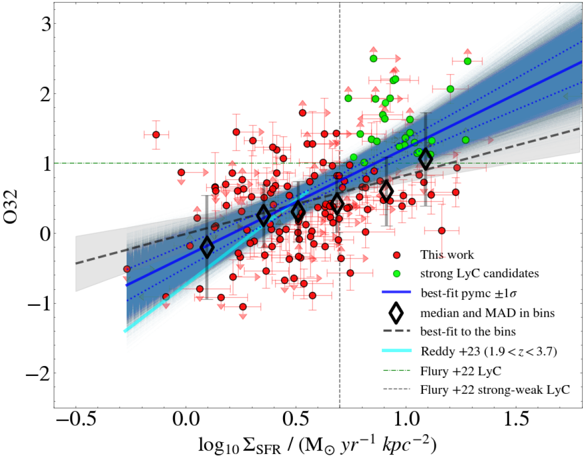
Figure 5: Figure displaying the $\Sigma_{\rm SFR}\$as a function of the O32 index for our selected sample in the entire range $4<z<10$. The lines, shaded areas, and markers are the same as in Fig. 2. The circles colored in lime green highlight our strong LyC leaking candidates, according to the criteria defined by Flury et al. (2022).

The SFR surface densities of galaxies have been shown recently to be tightly related and to have a key influence on their ionizing properties (Reddy et al., 2022). We know from simulations, galaxy models, and observations, that high redshift galaxies have higher ionization parameters (at fixed stellar mass) compared to local analogs (e.g., Brinchmann et al., 2008; Nakajima et al., 2013; Steidel et al., 2014; Kewley et al., 2015; Shapley et al., 2015; Hirschmann et al., 2017, 2023; Euclid Collaboration et al., 2024). This redshift evolution of ionization conditions is usually explained as a combined effect of lower metallicity, harder stellar ionizing spectra, and higher gas densities at $z>>0$. The latter increasing trend, also found with the electron density $n_{e}$ (Isobe et al., 2023), which is more easily measurable from optical emission lines, reflects the denser, more compact molecular clouds, and ultimately also higher values of $\Sigma_{\rm SFR}\$. Significant correlations were indeed found observationally between $n_{e}$ and $\Sigma_{\rm SFR}\$(Shimakawa et al., 2015; Jiang et al., 2019; Reddy et al., 2023), confirming the close relation between the two quantities, and the important role of $\Sigma_{\rm SFR}\$in the evolution of the ISM properties across cosmic time (see also Papovich et al. 2022).

We test here the connection between $\Sigma_{\rm SFR}\$and the ionization conditions, comparing the measured values of $\Sigma_{\rm SFR}\$to the O32 index, which is usually adopted as an observational proxy for the ionization parameter. The result is shown in Fig. 5. The O32 values, represented on the y-axis, range between $-0.3$ and $1.3$, with a median of $\sim 0.6$. We observe an increase of O32 with $\Sigma_{\rm SFR}\$, with a slope of $1.5\pm 0.2$, indicating that the correlation is statistically significant at more than $3\sigma$ level. We notice also that the galaxies in the top right part of the diagram, with $\Sigma_{\rm SFR}\$$\geq 1$ and O32 $\geq 0.7$, have similar properties to photometrically selected extreme emission line galaxies (EELGs) in the CEERS field at $z=$ $4$-$9$, recently presented by Llerena et al. (2023). We refer to that paper for a more detailed discussion. Overall, these findings corroborate previous results, supporting the close relation between $\Sigma_{\rm SFR}\$and the ionization properties of galaxies.

4.3 SFR surface density and escape of Lyman continuum photons

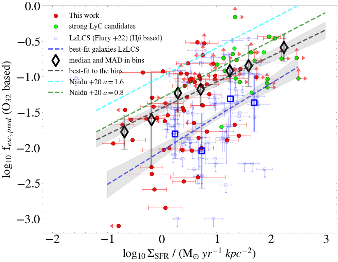
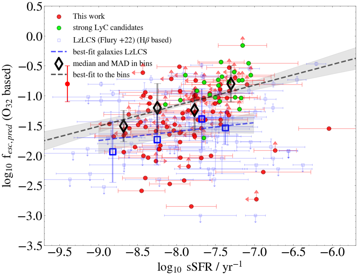
Figure 6: Top: Diagram comparing $\Sigma_{\rm SFR}\$and $f_{esc}\$for galaxies at $4<z<10$ with an estimate of $f_{esc}\$. The lines, shaded areas, and markers are the same as in Fig. 2. Bottom: sSFR vs $f_{esc}\$for this NIRSpec sample. The lime green circles represent strong LyC leaking candidates according to Flury et al. (2022), as highlighted in Fig. 5. The sample representative error of $0.3$ dex on $f_{esc}\$is added below the legend in each panel. We include with blue empty squares the LzLCS sample of $66$ galaxies at $0.2<z<0.4$, with measurements (including direct estimates of $f_{esc}\$) performed by Flury et al. (2022).

Enhanced values of the O32 index and $\Sigma_{\rm SFR}\$are usually associated with increased fractions of ionizing photons that escape from the galaxies. The connection between $\Sigma_{\rm SFR}\$(or O32) and $f_{esc}\$is found from multiple observations and with different approaches. Lyman continuum leaking sources (LyC), identified through direct or indirect methods, are found to have $\Sigma_{\rm SFR}\$ significantly higher than the average value of the star-forming population at a given redshift (e.g., Cen, 2020). In the other direction, galaxies with enhanced $\Sigma_{\rm SFR}\$ show larger fractions of LyC leakers. For example, Heckman (2001) and Heckman (2002) claim that galaxies with $\Sigma_{\rm SFR}\$above $0.1$ $M_{\odot}\$/yr/kpc² are capable to launch strong star-forming driven winds, which might be responsible for creating channels though which Lyc photons can leak. Steidel et al. (2018), based on a sample of LBGs at $z\sim 3$, suggest that $\Sigma_{\rm SFR}\$and $f_{esc}\$are highly correlated quantities. Similarly, the O32 index is considered as a valid indicator of LyC leaking, according to Izotov et al. (2020). Flury et al. (2022) also found that $40\%$ of local galaxies with $\Sigma_{\rm SFR}\$$>10$ $M_{\odot}\$/yr/kpc² and O32 higher than $0.7$ are LyC leakers, hence they adopted these two conditions at higher redshifts to define a source as a strong LyC leaker candidate.

Following these observational findings, hydrodynamical simulations and models have started to implement the effects of spatially concentrated star-formation in the form of turbulence and stellar-driven winds (Ma et al., 2016; Sharma et al., 2016), showing that an increased $\Sigma_{\rm SFR}\$is responsible for launching galaxy-wide outflows and for carving ionizing channels in the ISM where the Lyman continuum radiation of young massive stars and supernovae is free to propagate outside. According to the model of Naidu et al. (2020), $f_{esc}\$reaches unity when $\Sigma_{\rm SFR}\$is one-third of the maximum $\Sigma_{\rm SFR}\$($=1000$ $M_{\odot}\$/yr/kpc²) that can be sustained without radiation pressure instabilities (Hopkins et al., 2010).

Triggered by this extensive observational and theoretical background, we explore with our dataset the relation between $\Sigma_{\rm SFR}\$and $f_{esc}\$at redshifts $4<z<10$. We determine $f_{esc}\$in an indirect way using the empirical relation presented in Mascia et al. (2023), which provides an estimation of the escape fraction using three galaxy parameters: the UV beta slope, the physical size $r_{e}$, and the O32 index, which are amongst the properties better correlated with $f_{esc}\$. This relation is calibrated on the low-redshift Lyman Continuum survey (LzLCS), for which Flury et al. (2022) performed direct measurements of the Lyman continuum flux and $f_{esc}\$.

In Fig. 6-top, we show $\Sigma_{\rm SFR}\$as a function of $f_{esc}\$. Using our two analysis approaches, we find in all cases a significant correlation between these two parameters, according to which galaxies with higher $\Sigma_{\rm SFR}\$have systematically higher $f_{esc}\$than galaxies with lower $\Sigma_{\rm SFR}\$. In detail, $f_{esc}\$increases from $\log$ $\Sigma_{\rm SFR}\$$=-1$ to $3$, with a best-fit slope of $0.37\pm 0.05$ by fitting the median values in $7$ bins of $\Sigma_{\rm SFR}\$defined with the following grid [$-1$, $-0.5$, $0$, $0.5$, $1$, $1.5$, $2$, $3$]. This indicates that galaxies with more concentrated SFR have the conditions that should facilitate the escape of LyC photons. A subset of $\sim 20\%$ of our galaxy sample have $\Sigma_{\rm SFR}\$and O32 satisfying the conditions established by Flury et al. (2022) for being strong LyC leaker candidates, showing similar properties to the LyC leakers studied at redshift $\sim 0.3$. These systems, indicated with lime circles in Fig. 6 and in Fig. 5, tend to have higher $f_{esc}\$estimates compared to the average galaxy population at these redshifts.

We compare our observations to the direct measurements of $f_{esc}\$and physical properties estimated by Flury et al. (2022) for the LzLCS galaxy sample (blue empty squares in Fig. 6). We find a similar slope of the best-fit relation, even though we derive a higher normalization by $\sim 0.5$ dex. This might be related to a combination of factors, including the different redshift ranges probed by our works, and the different selection, as they select slightly more massive galaxies ($M_{\star}\$$>10^{8}$ $M_{\odot}\$).

We also find that the slope of our correlation is consistent with the $f_{esc}\$$\propto$ $\Sigma_{\rm SFR}\$^0.4 relation predicted by the Naidu et al. (2020) model. We find a lower normalization of our relation by $\sim 0.3$ dex compared to their fiducial model with $a=1.6$, possibly suggesting a lower value of this parameter. For completeness, we also report in Fig. 6-top the model with $a=0.8$, which is not ruled out in their work (as shown in their Fig. $6$), and whose prediction is much closer to our best-fit relation. However, their $f_{esc}\$vs $\Sigma_{\rm SFR}\$relation relies on measurements by Steidel et al. (2018), which are based on a sample of star-forming galaxies at redshift $z\sim 3$. The difference may thus originate from the different redshifts probed by our works.

A big caveat to the above analysis is that the two quantities on the x and y axis are not completely independent: $\Sigma_{\rm SFR}\$correlates with the size, while $f_{esc}\$is strongly dependent on the size by construction. While this is unavoidable, we also remark that the $f_{esc}\$estimation is based also on other galaxy properties and not just on the $r_{e}$. However, in order to provide a more independent measurement, we also compare the estimated values of $f_{esc}\$to the sSFRs, which do not directly depend on the physical extension of the galaxies (Fig. 6-bottom). We find that the sSFR is still correlated to $f_{esc}\$, although with a shallower slope and lower significance compared to the same relation with $\Sigma_{\rm SFR}\$. Also in this case the slope of our best-fit relation is similar to what is found for the LzLCS galaxy sample at $z\sim 0.3$, suggesting that the level of star-formation activity in a galaxy (regardless of the normalization method) has an impact on the escape of ionizing radiation. Overall, we are aware that all these quantities (i.e., $f_{esc}\$, $\Sigma_{\rm SFR}\$, sSFR, size, UV slope, and O32) are all interrelated somehow and not fully independent, as many of them depend on the same physical processes. This tells us that the best candidates as LyC leaking galaxies have rather peculiar and similar properties, being characterized by blue UV slopes, compact sizes, high O32, and also enhanced star-formation activity in the form of $\Sigma_{\rm SFR}\$and sSFR.

4.4 Connecting star-formation and outflows

We have seen in the previous section that $\Sigma_{\rm SFR}\$is tightly related to the ionizing properties of galaxies and their ability to spread ionizing photons in their surrounding medium. The underlying physical mechanism through which $\Sigma_{\rm SFR}\$impacts on $f_{esc}\$is that galaxies with more compact and enhanced star-formation activity facilitate the launch of galaxy scale outflows through stellar feedback, which includes radiation from young stars, stellar winds, and supernova explosions. Indeed, several studies in the literature have found higher gas outflow velocities and mass loading factors in galaxies with higher $\Sigma_{\rm SFR}\$(Llerena et al., 2022; Calabrò et al., 2022), corroborating the close relation between $\Sigma_{\rm SFR}\$and outflows. From the theoretical point of view, Sharma et al. (2016) and Sharma et al. (2017) predict that outflows are ubiquitous in galaxies with $\Sigma_{\rm SFR}\$$\geq 10$ $M_{\odot}\$/yr/kpc². In this subsection, we thus investigate spectral outflow signatures in our sample and study how they relate to the host galaxy properties. We also test the impact of outflows in an indirect way through the effect that they may have on the dust attenuation.

4.4.1 Exploring spectral outflow signatures in our sample

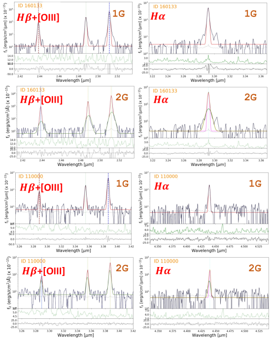
Figure 7: Diagrams showing the single Gaussian (1G) and double Gaussian (2G, narrow + broad) best fits to the [O iii] $\lambda 5007\AA$+H$\beta$ and H$\alpha$ lines, as indicated in each panel label, for the two galaxies (ID GLASS 160133 and 110000) in which we detect a significant outflow signature in both emission lines (upper and lower four panels, respectively). In each panel, the upper part shows the observed spectrum with the best fit line in red (red (green) line for the narrow (broad) component in the double Gaussian fit), the middle part represents the error spectrum, while the bottom part is the residual after subtracting the best fit result. The spectra are in the observed frame wavelength.

To study the presence of outflows of ionized gas, we use the GLASS high resolution grating spectra and perform a single Gaussian and a double-component (narrow+broad) Gaussian fit to the H$\alpha$ and [O iii] $\lambda 5007\AA$ lines (when available), which are the lines with the highest S/N in this redshift range, thus the most suited for exploring low S/N outflow features. In detail, H$\alpha$ was fitted alone, as the contribution from [N ii] $\lambda 6583\AA$ can be neglected at first order, while [O iii] $\lambda 5007\AA$ was fitted together with H$\beta$ and [O ii] $\lambda 4959\AA$ as explained in Section 2.2. In the double Gaussian fit, we add a second broad component, allowing the intrinsic velocity width $\sigma$ of the narrow component to vary between $10$ and $250$ km/s, and $\sigma$ of the broad component from $100$ to $800$ km/s, which is the limit expected for star-forming driven outflows (Calabrò et al., 2022). We constrain the velocity shift between the two Gaussian centroids to $<300$ km/s, of the same order of the spectral resolution. We do not set any constraints on the flux ratio of the two components. In case of the H$\beta$ + [O iii] triplet, a broad component is added to all the three lines. Finally, we consider the two component fit as successful if its reduced $\chi^{2}$ (i.e., $\chi^{2}_{red}$) is at least $10\%$ lower than the $\chi^{2}_{red}$ obtained with the single Gaussian fit, and if both the narrow and broad best-fit Gaussians are detected with a flux S/N $>3$.

With the above criteria, we find that a broad component is required to fit [O iii] and H$\alpha$ of two galaxies: ID 160133 and ID 110000 (Fig. 7). We primarily interpret these components as an outflow, with $\sigma_{broad}=$ $250\pm 4$ km/s and $200\pm 10$ km/s, respectively. We measure a broad to narrow line flux ratio of $0.16$ ($0.3$) and a broad to narrow $\sigma$ ratio of $3.4$ ($2.8$). These galaxies lie at redshifts $4.02$ and $5.76$, respectively, and both have a modest $\log$ $\Sigma_{\rm SFR}\$/($M_{\odot}\$yr^-1 kpc^-2) of $0.6\pm 0.2$ ($0.4\pm 0.2$), comparable to the average galaxy population at their redshifts, and $\log$ sSFR /(yr^-1) of $-7.6\pm 0.2$ ($-8.5\pm 0.3$). We also notice that both galaxies with outflow signatures show low surface brigthness clumpy structures around the main cores from high-resolution JWST images, which makes the scenario of gas accretion an interesting, alternative possibility that cannot be excluded with our spectroscopic data.

To better understand these results, we compare them to those obtained with a comparable dataset by Carniani et al. (2023), which includes $52$ galaxies with R$=2700$ spectra from the JWST-JADES program at redshifts, stellar masses, and SFRs similar to our work. They detect broad additional components in H$\alpha$ or [O iii] in a fraction of galaxies going from $15\%$ to $40\%$, which they interpret as evidence of outflows. They find that the outflow incidence increases with SFR but is rather stable (at the level of $20$-$30\%$) as a function of $M_{\star}\$and sSFR. Limiting the comparison to the redshift range between $4$ and $\sim 6$ (where most of their galaxies lie), and assuming the simple interpretation (also favored by their work) of an outflow scenario, we derive in GLASS an outflow incidence of $\sim 20\%^{32\%}_{9\%}$ ($2$ out of $11$ galaxies with detected [O iii]), with uncertainties derived following Gehrels (1986). This result is comparable to Carniani et al. (2023). We also notice that our flux and $\sigma$ ratios between the narrow and broad Gaussian components fall within their observed range. All this suggests that we are probably probing the same physical phenomenon. Interestingly, we do not observe instead any outflow signatures in the $6$ GLASS sources at $z>6$ (upper limit of $26\%$). In this case, we cannot make comparisons as this redshift range is poorly sample by the other work. Within our sample, the number of high redshift sources with high resolution spectra is so low that the outflow incidence at $z>6$ is still compatible with that derived at lower redshift. However, we can exclude from this analysis that outflows become more important at higher redshifts.

Furthermore, we do not find significant evidence of outflows in individual galaxies among the CEERS sample observed at medium resolution (R$\simeq 1000$). To understand whether this is expected, and to test the effect of resolution on the outflow detectability, we perform a set of Monte Carlo simulations. In detail, we simulate spectra at different redshifts injecting an emission line at a specific wavelength ($0.53\mu m$ rest frame) assuming different line fluxes to produce a variety of S/N of the emission feature (from $3$ to $\sim 60$). We also set a broad to narrow intrinsic flux ratio in the range between $0.1$ and $0.7$, and different $\sigma$ ratios ranging $2$ to $12$, with $\sigma_{narrow,intrinsic}$ fixed to $50$ km/s. We vary the intrinsic broad line centroid within a resolution element. We then perform a single Gaussian and double Gaussian (narrow + broad) fit as done for the observed data, imposing the same requirements for taking the double component as the final best fit. Running these simulations ($100$ for each configuration) we find that the recovery rate is of the order of $2\%$ or less for the typical range of outflow parameters expected from our works and from previous findings. This rate is not strongly dependent on the specific assumptions, except for the most extreme cases such as width and flux ratios $>=5$ and $>=0.5$, respectively. Therefore, the lack of significant outflow signatures in the CEERS sample is likely due to their lower spectral resolution.

Increasing the S/N of the emission lines, for example through spectral stacking, can slightly increase the outflow recovery rate at median resolution and the possibility of detecting faint broad components in case of high outflow velocities. We thus stack the entire dataset selected in this work with H- or M-grating observations. We first downgrade by convolution the GLASS high resolution spectra to R $=1000$, convert the spectra to rest-frame using the spectroscopic redshifts determined in Section 2.2, resample them to a common wavelength grid, and normalize them to the median flux estimated around the specific lines analyzed. Then, we apply for each pixel a median stacking with $5\sigma$ clipping, and finally perform the line measurements as done for individual galaxies. As shown by our simulations, this stacking approach tends to broaden a line systematically (regardless of the S/N or intrinsic line width) by $\sim 50$ km/s, as due to the impact of the spectral resolution on the redshift estimation uncertainty when converting to rest-frame.

Stacking the spectra around the [O iii] $\lambda 5007\AA$ line, which is the highest S/N line available for the largest number of galaxies in our sample, and fitting the H$\beta$ +[O iii] triplet with a single and double Gaussian as described before, we find a $\chi^{2}_{red,1G,2G}$ ratio ($=\chi^{2}_{red,1G}$ / $\chi^{2}_{red,2G}$) slightly below $1.1$, with a broad component $S/N$ of $2.9$, thus there is no significant evidence of outflow. Despite this, the resulting best double-component fit has a $\sigma_{broad}$ of $256$ km/s, consistent with the average outflow velocity width found for the JADES sample studied by Carniani et al. (2023). Given the lower S/N, we are not able to appreciate significant differences in the fit or to detect any outflow signatures if we divide the sample in two or more bins of redshift, sSFR, or $\Sigma_{\rm SFR}\$.

Overall, we find outflow incidence rates in individual galaxies observed by GLASS that are consistent to those obtained by similar works in the same redshift range. A larger sample of galaxies with high resolution NIRSpec data are certainly required to further constrain the incidence and outflow properties of galaxies during the reionization epoch, and most important their dependence on $\Sigma_{\rm SFR}\$and sSFR.

4.4.2 Investigating the attenuation and the outflow incidence of extremely star-forming galaxies

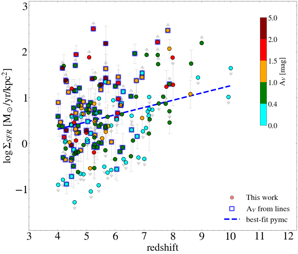
Figure 8: Redshift evolution of $\Sigma_{\rm SFR}\$(analog to Fig. 2), color coded by the attenuation A_V, estimated as described in the text. Galaxies with A_V derived from the emission lines are encapsulated within bigger blue squares.

Approaching the epoch of cosmic dawn, galaxies tend to have denser ISM and more concentrated star-formation activity, as shown in the previous sections. For electron densities exceeding $\sim 200$ cm^-3, the radiation pressure from young stars starts to dominate over the thermal pressure sustained by supernovae explosions (Ferrara, 2024). Assuming the $(1+z)^{p}$ redshift evolution of $n_{e}$, we expect this transition to occur for the average galaxy population in a redshift range between $3$ and $7$, depending on the value of the exponent $p$ between $1$ and $2$ (see Isobe et al. 2023). In these conditions of gas density and pressure, supernova explosions rapidly lose energy due to radiative losses, and the energy is converted into sound waves through shocks on a short timescale (see, e.g., Martizzi et al. 2015, Gatto et al. 2015, Kim & Ostriker 2015, Walch & Naab 2015, Fielding et al. 2017), making supernova-driven outflows highly inefficient in early galaxies. Some theoretical models predict that in compact galaxies with extreme star-formation activity, a super-Eddington regime could be established, according to which radiation driven outflows can dramatically decrease the dust optical depth by pushing it to larger radii in a few Myr (Ferrara, 2024). This drastic event is expected when the sSFR exceeds $\sim 10^{-7.6}$ yr^-1. The consequence of this process is the formation of a system that has negligible dust attenuation, hence a very blue SED. This model was introduced to explain the excess of UV-bright and blue galaxies (compared to theoretical expectations) discovered during the first JWST observing campaigns (e.g., Naidu et al., 2022; Castellano et al., 2022), however it is still unclear whether it is the right physical explanation to the observational findings, and when exactly this proposed mechanism might start to dominate.

To test this scenario we analyze the outflow incidence rate in galaxies with extremely high sSFR. First, we find that the fraction of galaxies in super Eddington regime (i.e., sSFR $>10^{-7.6}$ yr^-1) in all the redshift range explored in this work ($4<z<10$) is consistent with the model predictions by Ferrara (2024), increasing from $\sim 15\%$ at redshift $4$ to $\sim 40\%$ at redshift $10$. Among these galaxies, if we consider only those $5$ observed by GLASS at high resolution, we find an outflow incidence rate of $1$/$5$ ($\sim 20\%$), or $1$/$3$ if we limit the analysis to systems with a compact morphology, that is, with an effective radius of $150$ pc or less. In both cases, these fractions are compatible with the incidence rate obtained from the full sample.

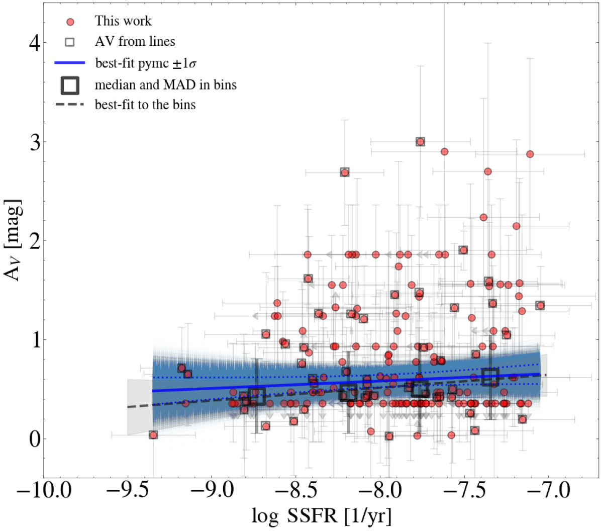
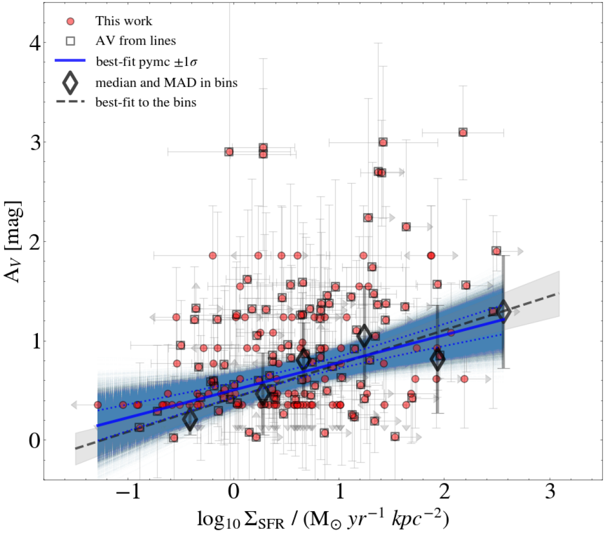
Figure 9: Diagrams comparing A_V to sSFR and $\Sigma_{\rm SFR}\$(top and bottom panels, respectively) for our selected galaxies in the redshift range $4<z<10$. The lines, shaded areas, and markers are the same as in Fig. 2.

An alternative method to test the effect of star-formation on the dust content of galaxies, including the dust clearing scenario, is to analyze how the galaxy attenuation A_V is related to the star-forming properties. To this aim, in Fig. 8, we color code the points in the $z$-$\Sigma_{\rm SFR}\$diagram as a function of A_V. We can see that galaxies at $z>7$ have a large variety of A_V: while some galaxies have upper limits on A_V consistent with $0$, some others have higher values that can reach A${}_{V}=2$ magnitudes. Therefore, we do not see evidence for a sudden drop of A_V with redshift down to the very low values (A_V $\simeq 10^{-2}$-$10^{-3}$) expected by the dust-clearing scenario, nor that the global galaxy population at $z>7$ is dominated by systems with A${}_{V}\simeq 0$, even if the majority of this high-$z$ subset also has sSFRs largely exceeding the super-Eddington conditions defined above.

We can better understand this result by plotting A_V as a function of sSFR for the entire redshift range (top panel of Fig. 9). We can see that galaxies with higher sSFR show a large variety of A_V. Globally, the median A_V slightly increases with sSFR but it is consistent also with a flat relation ($m=0.07\pm 0.09$). In the bottom panel of Fig. 9 we analyze instead the relation between A_V and $\Sigma_{\rm SFR}\$. Here we find a positive correlation between the two quantities, with a best-fit slope of $0.28\pm 0.07$ with the Bayesian method, indicating that galaxies with more concentrated star-formation (i.e., higher $\Sigma_{\rm SFR}\$) have higher dust attenuations on average. This positive correlation is similar to what is found in lower redshift studies (e.g., Reddy et al., 2015; Tomičić et al., 2017), and it reflects the fact that galaxies accumulate more dust in their ISM as a consequence of their increased (and more compact) star-formation activity. Dividing our sample in two redshift bins (lower and higher than $6$), we find no significant differences in the global trends seen in both panels of Fig. 9.

In conclusion, we can hypothesize several different explanations to our results. First, if the dust clearing radiatively driven outflows (in super Eddington conditions) play an important role in galaxy evolution, they might start to dominate at redshifts higher than $10$. We should note that the two NIRSpec galaxies at $z\simeq 10$ in our sample are both dust poor, consistent with this scenario, while we do not have statistics at $z>10$. We are focusing instead on a cosmic epoch where the feedback from supernovae is likely contributing to the acceleration of winds, as incorporated in several models and simulations (e.g., Sharma et al., 2017). Therefore, supernovae feedback remains the most plausible explanation for the outflows observed in NIRSpec galaxies at $z<6$. However, we should also be aware of the possible lesser role played by supernovae as we approach the reionization epoch, following the argument explained above. Galaxies at cosmic dawn are also expected to be younger than analogs at lower redshifts, with consequently shorter times available to supernovae to impact the surrounding ISM in a stable way. Moreover, the relatively low outflow incidence might also reflect geometry effects.

Secondly, the fraction of halo gas entrained by the outflowing shell might be conspicuous at the level of $10\%$ or more. Consequently, the gas outflow velocities can be relatively low (see equation 15 in Ferrara 2024), to the level of $50$-$100$ km/s that are not easily detectable even in high resolution spectral mode. Another alternative explanation is that we are observing the galaxies in an intermediate phase of dust accumulation, possibly coincident with a period of gas accretion and dust creation by the first star formation episodes, that has not yet reached the conditions of dust opacity for developing a sudden blow-out event. In this particular phase, whose duration is not well known, the galaxies might still retain most of their gas and dust content, showing attenuations significantly higher than $0$ while keeping a low-level outflowing activity.

5 Summary

We summarize the main findings of this paper as follows. We analyze a spectroscopic sample of galaxies in the redshift range from $4$ to $10$ observed with JWST-NIRSpec by the CEERS and GLASS surveys. Using the Balmer lines and UV-based effective radii, we study the evolution of the SFR and $\Sigma_{\rm SFR}\$over this cosmic epoch.

1. We find that $\Sigma_{\rm SFR}\$increases mildly in this redshift range (best-fit slope $=0.16\pm 0.06$), rising by a factor of $2$ from $z=4$ to $10$. This trend is consistent with the predictions from several semi-analytic models of galaxy evolution, such as the Santa Cruz models (Somerville & Davé, 2015), and those by Ferrara (2024) and Naidu et al. (2020).

2. A star-forming ‘Main Sequence’ relation holds out to redshift $\sim 10$, with a best-fit slope of $\sim 0.7$, consistent with the relations obtained for star-forming galaxies at lower redshifts.

3. We derive for the first time at $z>4$ the $\Sigma_{\rm SFR}\$‘Main Sequence’, finding a very mild increase (consistent with a flat relation) of $\Sigma_{\rm SFR}\$with stellar mass. The slope of the best-fit relation is in agreement with observations at $0<z<2$, while the normalization is about $\sim 2.5$ dex higher (at $z\sim 10$) compared to the local Universe, resulting from the strong evolution of the average $\Sigma_{\rm SFR}\$in star-forming galaxies during the last $13$ Billion years.

4. We show that $\Sigma_{\rm SFR}\$is tightly related to the ionizing source properties, probed by the O32 index. This corroborates recent studies proposing $\Sigma_{\rm SFR}\$as a key quantity responsible for the higher ionization parameter observed in high redshift galaxies (Reddy et al., 2023).

5. We find correlations of $\Sigma_{\rm SFR}\$and sSFR with the escape fraction, estimated in an indirect way using the prescription of Mascia et al. (2023) calibrated on direct measurements of $f_{esc}\$from the low-redshift Lyman continuum survey (Flury et al., 2022). The slopes of both correlations are in agreement with observations of low-redshift LyC leakers and with those predicted by the models of Naidu et al. (2020).

6. We detect outflow signatures in H$\alpha$ and [O iii] $\lambda 5007\AA$lines for $\sim 20\%$ of the galaxies at $z<6$ observed in H-grating NIRSpec mode, in agreement with the outflow incidence found in galaxies at similar redshifts by Carniani et al. (2023).

7. We find a positive correlation between A_V and $\Sigma_{\rm SFR}\$, and a flat trend as a function of sSFR, indicating that there is no evidence of a drop of A_V in extremely star-forming galaxies between $z=4$ and $10$. This might be at odds with a dust-clearing outflow scenario, which might instead take place at redshifts $z\geq 10$, as suggested by some theoretical models.

Observing a larger number of galaxies at high resolution and testing the correlation between $\Sigma_{\rm SFR}\$and outflow velocity predicted by supernovae feedback models can help us in the future to further constrain the properties and physical origin of the outflows detected both in our and in similar works at $z\sim 4$ to $10$, and further clarify the relation between star-formation and outflows in the epoch of reionization. Enlarging the sample of spectroscopically confirmed galaxies at $z>10$ is also essential to test possible transformations of the ISM properties occurring at this cosmic epoch.