DUVET: sub-kiloparsec resolved star formation driven outflows in a sample of local starbursting disk galaxies

Abstract

We measure resolved (kiloparsec-scale) outflow properties in a sample of 10 starburst galaxies from the DUVET sample, using Keck/KCWI observations of H$\beta$ and [OIII] $\lambda$5007. We measure $\sim 450$ lines-of-sight that contain outflows, and use these to study scaling relationships of outflow velocity ($v_{\rm out}$), mass-loading factor ($\eta$; mass outflow rate per SFR) and mass flux ($\dot{\Sigma}_{\rm out}$; mass outflow rate per area) with co-located SFR surface density ($\Sigma_{\rm SFR}$) and stellar mass surface density ($\Sigma_{\ast}$). We find strong, positive correlations of $\dot{\Sigma}_{\rm out}\propto\Sigma_{\rm SFR}^{1.2}$ and $\dot{\Sigma}_{\rm out}\propto\Sigma_{\ast}^{1.7}$. We also find shallow correlations between $v_{\rm out}$ and both $\Sigma_{\rm SFR}$ and $\Sigma_{\ast}$. Our resolved observations do not suggest a threshold in outflows with $\Sigma_{\rm SFR}$, but rather we find that the local specific SFR ($\Sigma_{\rm SFR}/\Sigma_{\ast}$) is a better predictor of where outflows are detected. We find that outflows are very common above $\Sigma_{\rm SFR}/\Sigma_{\ast}\gtrsim 0.1$ Gyr^-1 and rare below this value. We argue that our results are consistent with a picture in which outflows are driven by supernovae, and require more significant injected energy in higher mass surface density environments to overcome local gravity. The correlations we present here provide a statistically robust, direct comparison for simulations and higher redshift results from JWST.

1 Introduction

The evolution of galaxies is shaped by the baryon cycle. Cold gas is accreted onto galaxies, used as fuel in star formation which in turn enriches the gas, and is then ejected from the galaxy to enrich the surrounding environment (Somerville & Davé, 2015). Star formation-driven outflows are a necessary component of this cycle, contributing to the enrichment of the circumgalactic medium (CGM) (Tumlinson et al., 2017; Cameron et al., 2021), and suppressing star formation through the removal of gas (Veilleux et al., 2005; Bolatto et al., 2013; Reichardt Chu et al., 2022b). Galaxy-wide outflows are required for simulations to reproduce basic galaxy properties including the galaxy mass function, typical galaxy sizes, and the Kennicutt-Schmidt Law (e.g Springel & Hernquist, 2003; Oppenheimer & Davé, 2006; Hopkins et al., 2012, 2014). To constrain the implementation of galaxy-wide outflows in simulations, the simulations need to be compared to empirical measurements of outflow quantities. It is, therefore, necessary that we understand the observational properties of outflows and their driving mechanisms.

Star formation-driven outflows have been observed across cosmic time (e.g. Heckman et al., 2000; Chen et al., 2010; Rubin et al., 2010; Davies et al., 2019). Outflows are an observational tracer of the feedback process that regulates star formation, preventing runaway star formation in multiple ways. First, it is expected that the gravitational weight of the disk creates pressure in the interstellar medium (ISM) which is balanced by the energy and momentum injected into the ISM by young massive stars and supernovae. This injected energy and momentum creates turbulence, suppressing the star formation occurring within the galaxy disk (e.g. Ostriker et al., 2010; Faucher-Giguère et al., 2013; Hayward & Hopkins, 2017; Krumholz et al., 2018; Ostriker & Kim, 2022). Recent observations that compare velocity dispersion to the star formation properties find correlations that are consistent with feedback-based regulation of star formation in disks (Fisher et al., 2019; Girard et al., 2021). Pre-supernova feedback from young massive stars affects the density of the ISM gas that the supernovae then explode into, regulating the impact of the supernova feedback (McLeod et al., 2021; Chevance et al., 2022). In more extreme starburst environments, clustered supernovae create expanding “superbubbles” which drive galactic winds when they break out of the disk (Fielding et al., 2018; Kim & Ostriker, 2018; Vijayan et al., 2020; Orr et al., 2022). Once these expanding gas bubbles break out of the disk, the gas they drive out of the galaxy is no longer available for star formation. Scaling relations are useful for identifying where this occurs, and in which local regions the outflow dominates over turbulence as the main method of star formation regulation. Moreover, establishing observational scaling relations provides direct tests for simulations (e.g. Kim et al., 2020; Rathjen et al., 2023).

Simulations make direct predictions of outflow properties such as the outflow velocity $v_{\rm out}$, the outflow mass flux $\dot{\Sigma}_{\rm out}$, and the mass loading factor $\eta$ as a function of the star formation rate surface density $\Sigma_{\rm SFR}$ (e.g. Nelson et al., 2019; Kim et al., 2020; Pandya et al., 2021). Characterising these scaling relationships provides constraints on our understanding of the physical drivers of outflows. For example, the relationship between the star formation rate surface density and the outflow velocity provides constraints on the primary driving mechanism of the outflows. Outflows primarily driven by mechanical energy from supernovae are expected to have a shallow relationship as $v_{\rm out}\propto\Sigma_{\rm SFR}^{0.1}$ (Chen et al., 2010; Li et al., 2017; Kim et al., 2020). However, if the outflows are primarily driven by momentum given to the gas by radiation from young massive stars, then the expected relationship has a steeper dependence as $v_{\rm out}\propto\Sigma_{\rm SFR}^{2}$ (Murray et al., 2005; Kornei et al., 2012; Hopkins et al., 2012). Outflows are almost certainly driven by a combination of both of these mechanisms. Spatial and temporal differences in the preprocessing of the ISM material that SNe explode into and entrain will contribute to the observed $v_{\rm out}-\Sigma_{\rm SFR}$ relationship. In addition, supernovae generate cosmic rays which are also expected to play a role in driving outflows (e.g. Girichidis et al., 2016, 2024). The extent to which this is important is unclear due to uncertainties in the parameters of cosmic ray transport (e.g. Naab & Ostriker, 2017; Crocker et al., 2021; Kim et al., 2023). To drive realistic galaxy-wide outflows, simulations need to include empirically motivated prescriptions that include the effects from all of the relevant feedback processes. As an initial constraint, these very different power-laws make observational tests of the primary contributor of the two models possible.

Observations of outflows have historically been limited by their low surface brightness to studies of either integrated galaxy samples, or stacked galaxy samples. Trends between the outflow velocity and global galaxy measurements of stellar mass, SFR and $\Sigma_{\rm SFR}$ of galaxies have been reported by many studies (e.g. Martin, 2005; Rupke et al., 2005; Steidel et al., 2010; Chen et al., 2010; Newman et al., 2012; Kornei et al., 2012; Arribas et al., 2014; Bordoloi et al., 2014; Rubin et al., 2014; Chisholm et al., 2015, 2017; Förster Schreiber et al., 2019). However, galaxy-wide observations have an underlying dependence on the stellar mass of the galaxy (Newman et al., 2012; Chisholm et al., 2015; Nelson et al., 2019), making it difficult to test the predicted local correlations. Moreover, it has not been established how the resolved measurements may alter empirical correlations between outflow and the galaxy from which they launched. For example, if outflows are launched from small-scale regions in a galaxy, then global averages may wash out any existing local relationships. Alternatively, it may be that aggregate effects of the wind dominate the outflow energetics, and thus global averages are more important.

Resolved observations of face-on galaxies allow the comparison of outflow properties to co-located galaxy properties. Using resolved observations, we can trace the outflowing kinematics back to the local energy and momentum injected by star formation to test on which scales the star formation drives galaxy-scale outflows. Recently developed sensitive IFUs, such as KCWI, MUSE and JWST/NIRSpec, have made this possible. In Reichardt Chu et al. (2022a) (hereafter RC22a) we studied resolved ionised outflows in the pilot target for the DUVET sample, IRAS 08339+6517. We found a shallow correlation between the local co-located $\Sigma_{\rm SFR}$ and $v_{\rm out}$, consistent with trends expected from supernovae being the primary outflow driving mechanism. In our follow-up paper, Reichardt Chu et al. (2022b) (hereafter RC22b), we found a relationship between the star formation rate surface density and outflow mass flux of $\dot{\Sigma}_{\rm out}\propto\Sigma_{\rm SFR}^{1.06\pm 0.1}$. In this paper, we extend this analysis to a sample of ten face-on galaxies from the DUVET survey.

The paper is organised as follows. We describe our galaxy sample in Section 2.1, and our observations and data reduction of the sample in Sections 2.2 and 3.1. We describe our method to fit for outflows in Section 3.2. The resulting relationships of the maximum outflow velocity, mass outflow flux, and mass loading factor with SFR surface density and stellar mass surface density are explored in Section 4. Conclusions are presented in Section 5. Throughout the paper, we assume a flat $\Lambda$CDM cosmology with $H_{0}=69.3$ km Mpc^-1 s^-1 and $\Omega_{0}=0.3$ (Hinshaw et al., 2013).

2 Observations and Data Reduction

2.1 DUVET sample

DUVET (Deep near-UV observations of Entrained gas in Turbulent galaxies) is a sample of starbursting disk galaxies at $z\sim 0.02-0.04$. The sample contains both face-on and edge-on galaxies so that we can build a three-dimensional understanding of the impact of stellar feedback and star formation-driven outflows on galaxies with high star formation rate surface densities, $\Sigma_{\rm SFR}$, and their environments (e.g. face-on: ; ; edge-on: Cameron et al. 2021; McPherson et al. 2023, McPherson et al. in prep). The galaxies are chosen to have total SFRs at minimum $5\times$ the main sequence value for their total stellar mass. The galaxies are also required to have the morphology and kinematics of a disk so that we can remove the underlying velocity field. The total sample has 27 galaxies and a stellar mass range of $10^{9}-10^{11}$ M_⊙.

This work uses 10 targets from the DUVET sample that have low inclinations. Inclination is estimated photometrically using the ratio of the major-to-minor axis in near-IR broadband images from 2MASS and Spitzer/IRAC ch1. Nine of these targets have inclinations of $i<15^{\circ}$, and one target is moderately inclined (CGCG 453-062: $i=54^{\circ}$). The inclined target was observed due to a range in LST at the time of observation that did not have sufficient targets available that meet the DUVET sample selection criterion. We will highlight CGCG 453-062 in our discussion of results and in the main results plots.

The ten galaxies chosen for this work span four orders-of-magnitude in $\Sigma_{\rm SFR}$ ($\sim 0.001-10$ M_⊙ yr^-1 kpc^-2) in $\sim 500$ pc scale regions, while keeping the total galaxy stellar mass $10-200\times 10^{10}$ M_⊙. Properties for all 10 galaxies examined here are given in Table 1, in order of increasing total stellar mass. We have calculated the infrared SFR (Column 5) using the standard Band 4 photometry from the WISE Telescope (Wright et al., 2010) given in the AllWISE Source Catalog (Cutri et al., 2021), following the relationship from Cluver et al. (2017, their Eq. 7). The profile-fit magnitudes from the AllWISE Catalog systematically underestimate the brightness of extended sources with respect to the WISE point spread function, and so the SFRs we calculate here are lower bounds.

Name	$z$	M∗	SFR${}_{\rm IFU,H\beta}^{*}$	SFRtotal,IR	$A_{v}$	$r_{50}$	$r_{90}$	$\log$ [OIII]/H$\beta$	References
		($10^{10}~{}M_{\odot}$)	($M_{\odot}$ yr-1)	($M_{\odot}$ yr-1)	(mag)	($\arcsec$)	($\arcsec$)
(1)	(2)	(3)	(4)	(5)	(6)	(7)	(8)	(9)	(10)
IRAS 08339+6517	0.019	1.10	11.1	20.5	$0.5^{+2.4}_{-0.5}$	2.6	5.9	$0.14\pm 0.05$	1
IRAS 15229+0511	0.036	3.02	4.7	20.6	$0.9^{+1.0}_{-0.9}$	3.7	9.1	$-0.34\pm 0.03$	2
KISSR 1084	0.032	3.05	3.5∗	5.4	$1.1\pm 0.5$	4.8	8.2	$-0.39\pm 0.03$	3
NGC 7316	0.019	4.17	3.8∗	2.9	$0.5^{+0.6}_{-0.5}$	6.8	12.3	$-0.24\pm 0.02$	4
UGC 01385	0.019	4.74	7.1	16.8	$1.2\pm 0.9$	2.8	7.6	$-0.32\pm 0.06$	5
UGC 10099	0.035	5.73	5.1	12.8	$0.3\pm 0.3$	2.5	6.2	$-0.06\pm 0.02$	6
CGCG 453-062	0.025	8.99	22.4∗	13.9	$1.9\pm 0.6$	7.2	13.2	$-0.48\pm 0.02$	5
UGC 12150	0.021	11.0	20.2∗	18.5	$4.0\pm 1.1$	5.3	11.1	$-0.40\pm 0.04$	5
IRAS 20351+2521	0.034	11.2	26.1∗	38.1	$1.3\pm 0.8$	7.3	12.1	$-0.19\pm 0.02$	7
NGC 0695	0.032	20.1	42.1∗	41.4	$1.8\pm 0.6$	5.9	11.2	$-0.23\pm 0.03$	5

Table 1: Columns are: (1) Galaxy name. (2) Redshift. (3) Stellar mass from literature, references given in Column 10. (4) Star formation rate from ionised gas using the H$\beta$ line. (5) Star formation rate from WISE Band 4 data, following Cluver et al. (2017, their Eq.7). (6) Average extinction in the disk gas based on the H$\gamma$/H$\beta$ flux ratio. (7) and (8) effective radius and 90% radius in arcseconds from g-band PanSTARRS data respectively. (9) Median $\log_{10}($[OIII] $\lambda 5007/$H$\beta)$ flux ratio. (10) References: 1–Fisher et al. (2022), 2–Bik et al. (2022), 3–Cook et al. (2019) 4–Fernández Lorenzo et al. (2013), 5–Howell et al. (2010), 6–Kouroumpatzakis et al. (2021), 7–Shangguan et al. (2019).
^∗ We use the total flux measured in H$\beta$ to calculate SFR_IFU,Hβ, however, some galaxies in our sample extend beyond the FOV of our observations and so this is a lower limit of the total SFR for the galaxy. The affected SFR values are indicated using an asterisk.

2.2 Observations

The galaxies were observed with KCWI/Keck II (Morrissey et al., 2018) over a range of nights given in Table 2, with sub-arcsecond seeing conditions. We used the BM grating in the large IFU slicer mode, giving a field of view of $20\aas@@fstack{\prime\prime}4\times 33\aas@@fstack{\prime\prime}$ with spatial sampling of $0\aas@@fstack{\prime\prime}29\times 1\aas@@fstack{\prime\prime}35$, which is seeing limited in the short spaxel side direction. The galaxies were observed using a half-slice dither pattern in the direction of the long side of the spaxel to allow for better spatial sampling. The exposure time and number of exposures for each galaxy are given in Column 3 of Table 2. All galaxies are observed with multiple grating settings a “blue" and “red" setting. In this paper we only use the red setting. The central wavelength set for the BM grating of the red setting is given in Column 4 of Table 2 for each galaxy and was chosen to include all wavelengths from H$\gamma$ to [OIII] $\lambda 5007$. The galaxies were also observed with a “blue” configuration, to extend the wavelength coverage from H$\gamma$ to below the [OII] doublet. The observations using the “blue" configuration are described in McPherson et al. in prep. A separate sky field was observed beyond the virial radius for each galaxy either directly before or after the science exposures. The observations and data reduction for the pilot target, IRAS 08339+6517 were discussed in detail in RC22a and Fisher et al. (2022). The observations and data reduction for the remaining nine galaxies follow a similar method.

The data were reduced using the standard IDL KCWI Data Extraction and Reduction Pipeline (Version 1.1.0). Before combining the images, small-scale imperfections in the WCS were accounted for by a re-alignment based on the H$\gamma$ emission line, which is detected in all images and allows for alignment with bluer wavelength settings taken on each galaxy not used in this work. The H$\gamma$ flux was compared in each pixel using an iterative minimisation method, and the WCS of the images was adjusted to result in the minimum average residual across each galaxy. The python package Montage was then used to reproject the images to produce square spaxels of $0\aas@@fstack{\prime\prime}29\times 0\aas@@fstack{\prime\prime}29$, based on the shorter side length of the original rectangular spaxels. The resulting reprojected images of each galaxy were co-added in Montage using the adjusted WCS coordinates. The variance cubes were similarly reprojected and coadded. The number of images and their exposure times are given in Column 3 of Table 2 for each galaxy. The reduction process for DUVET galaxies is described in more detail in McPherson et al. (2023).

To account for the (on average) $0\aas@@fstack{\prime\prime}7$ seeing conditions, the resulting realigned, reprojected and coadded cubes were binned $3\times 3$ to obtain cubes with a final spaxel size of $0\aas@@fstack{\prime\prime}87\times 0\aas@@fstack{\prime\prime}87$, which is comparable to the typical seeing FWHM. The dither pattern of the observations in the direction of the long side of the original spaxels ($0\aas@@fstack{\prime\prime}29\times 1\aas@@fstack{\prime\prime}35$) allows for the reconstructed images to better sample the seeing. RC22a found stronger correlations between outflow and co-located galaxy parameters above a re-binned spaxel size of ${\sim 0.5}$ kpc, and discussed possible geometric and temporal causes (see RC22a for a discussion). The reprojected spaxel size for the galaxies in this work is equivalent to $0.34$ kpc $\times~{}0.34$ kpc at $z=0.019$ for our closest galaxies and $0.63$ kpc $\times~{}0.63$ kpc at $z=0.036$ for our furthest galaxy. Our pilot target IRAS 08339+6517 is the exception to this, retaining its original data reduction from RC22a resulting in rectangular spaxels of $0\aas@@fstack{\prime\prime}3\times 1\aas@@fstack{\prime\prime}35$ ($0.1$ kpc$\times 0.5$ kpc at $z=0.019$).

Name	RA	Dec	Obs date	Exp times	Central wavelength
	(J2000)	(J2000)		(s)	(Å)
(1)	(2)	(3)	(4)	(5)	(6)
IRAS 08339+6517	08:38:23.18s	+65:07:15.2s	15 Feb 2018	1200, 600, 300, 100	4800
CGCG 453-062	23:04:56.53s	+19:33:08.0s	20 Oct 2019	$6\times 300$	4800
UGC 01385	01:54:53.79s	+36:55:04.6s	20 Oct 2019	$6\times 300$	4800
UGC 12150	22:41:12.26s	+34:14:57.0s	21 Oct 2019	$6\times 300$	4800
NGC 0695	01:51:14.24s	+22:34:56.5s	21 Oct 2019	$4\times 300$	4800
NGC 7316	22:35:56.34s	+20:19:20.1s	20 & 21 Oct 2019	$1\times 200,6\times 300,3\times 500$	4800
IRAS 15229+0511	15:25:27.49s	+05:00:29.9s	22 March 2020	$6\times 300$	4850
UGC 10099	15:56:36.40s	+41:52:50.5s	22 March 2020	$6\times 300$	4850
IRAS 20351+2521	20:37:17.72s	+25:31:37.7s	16 May 2020	$6\times 300$	4820
KISSR 1084	16:49:05.27s	+29:45:31.6s	16 May 2020	$6\times 300$	4820

Table 2: Columns are: (1) Galaxy name. (2) and (3) RA and Dec from NED*. (4) The date the galaxy was observed with KCWI/Keck II. (5) Number and length of exposure times in seconds. (6) is the set central wavelength of the BM grating.
*The NASA/IPAC Extragalactic Database (NED) is funded by the National Aeronautics and Space Administration and operated by the California Institute of Technology.

3 Methods

3.1 Continuum Subtraction

Before each cube was continuum subtracted, foreground extinction due to the Milky Way was corrected using the Cardelli et al. (1989) law and a galactic extinction value of 0.251 mag (Schlafly & Finkbeiner, 2011).

The full spectrum fitting code pPXF (Cappellari, 2017) was used to fit the stellar continuum. For this fitting to occur, the continuum was required to have a signal-to-noise greater than 3 in a continuum band (4600 Å $<\lambda<4800$ Å) for each galaxy data cube. For nine of the ten galaxies in this work, the continuum fitting used semi-empirical templates from Walcher et al. (2009). Emission line ratios of the galaxies suggest that IRAS 08339+6517 López-Sánchez et al. (2006) has a lower metallicity than the remainder of the sample. Due to this difference, and to keep consistency with the results from RC22a and RC22b, the continuum subtraction for IRAS 08339+6517 used the BPASS templates (Version 2.2.1, Stanway & Eldridge, 2018), including binary systems with a broken power-law initial mass function with a slope of -1.3 between $0.1~{}M_{\odot}$ and $1.0~{}M_{\odot}$, a slope of -2.35 above $1.0~{}M_{\odot}$, and an upper limit of $300~{}M_{\odot}$. The BPASS templates were built to cover younger ages and lower metallicities than the Walcher et al. (2009) templates.

Post continuum subtraction, we identified some spaxels where a wide residual absorption feature near H$\beta$ is not fully removed through the continuum subtraction process. This does not occur in all spaxels, and appears to be more common in more heavily extincted systems. The continuum subtraction of starburst galaxies is unreliable, due to well-known issues in creating stellar population libraries to model the continuum in these environments (Conroy, 2013). We therefore address any regions that were poorly fit by fitting any remaining residuals. Using short wavelength bands on either side of the emission lines, we fit a linear function across [OIII] $\lambda 5007$ and a quadratic across H$\beta$ such that the corrected spectrum has a flat baseline. The quadratic across H$\beta$ is fit at least 10 Å away from the emission line, and the correction is interpolated across the baseline. We use a quadratic function across H$\beta$ as it is more likely to be affected by residual hydrogen absorption in stellar photospheres. The resulting baselines are visually inspected for a subset of spaxels in each galaxy. We tested our results with and without this additional baseline correction and found the change fell within the error bars for the difference in both median outflow velocity and median outflow mass flux. Including the baseline correction decreased the median mass loading factor by $\sim 7\%$.

Finally, an internal extinction correction was calculated on a spaxel-by-spaxel basis for all galaxies using the emission line ratio H$\beta$/H$\gamma$ and the Calzetti (2001) extinction curve. This extinction correction was applied when calculating the star formation rate and the mass outflow rate. The impacts of including an extinction correction within the outflow mass calculation are discussed further in Section 4.2.

3.2 Emission-line Fitting Method

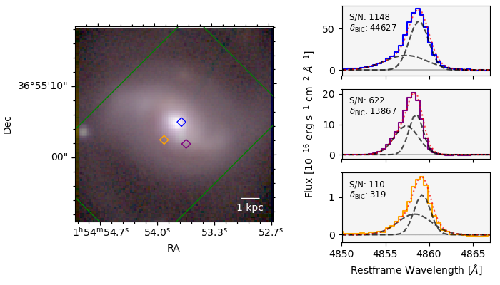
Figure 1: Example fits from DUVET target UGC 01385. Left panel: an RGB image of UGC 01385 (R: Pan-STARRS z-band, G: Pan-STARRS r-band, B: Pan-STARRS g-band). Large green rectangle shows the footprint of our KCWI observations. Blue, purple and orange small squares show highlighted KCWI spaxels, for which the H$\beta$ emission line fits are shown in the right-hand panels. Right-hand panels: for each panel, data is in blue, purple or orange corresponding to the squares in the left panel. The variance is shown as a grey band. Dashed black lines show the two-component Gaussian fits. Dotted red line shows the complete fitted model. The signal-to-noise and $\delta_{\rm BIC}$ are given for each spaxel (see Sec. 3.2 and Appendix A for more discussion of the $\delta_{\rm BIC}$).

To identify outflows we follow the method developed in previous DUVET papers (Reichardt Chu et al., 2022a; McPherson et al., 2023). We implement multi-component Gaussian fitting using the Python package threadcount, which uses the Python fitting package lmfit (Newville et al., 2019) with a Nelder-Mead simplex minimisation algorithm. We fit both a single and a double Gaussian to the H$\beta$ and [OIII] $\lambda$5007 emission lines independently in spaxels where we measure a signal-to-noise greater than 10 in the emission line. To determine whether the extra Gaussian component is necessary, we use the Bayesian information criterion (BIC). The form of the BIC we use here is the Aikake information creiterion, the special case where each model is fit to the same number of data points, defined as

$$BIC=\chi^{2}+2N_{\rm variables},$$ (1)

where $\chi^{2}=\sum(f_{\rm data}-f_{\rm model})^{2}/\sigma^{2}$, and $\sigma$ is the data uncertainty. $N_{\rm variables}$ is the number of variables included in the fit, which is 4 for single Gaussian fits and 7 for double Gaussian fits. Some example fits are shown for one of our targets, UGC 01385, in Fig. 1.

The double Gaussian model is only chosen where it gives a lower BIC value than the single Gaussian model minus a threshold value such that $BIC_{\rm doubleGaussian}<BIC_{\rm singleGaussian}-\delta_{\rm BIC}$. The threshold value, $\delta_{\rm BIC}=-200$, is discussed further in Appendix A. We restrict the double Gaussian fits such that the bluer component must have a smaller amplitude and larger velocity dispersion than the redder component. When a double Gaussian model is the statistically preferred fit, we assume the broad, blue-shifted component measures flux from outflowing gas and the narrower, higher amplitude component measures flux from gas within the galaxy disk (see ; and McPherson et al. 2023 for more detail). A visual inspection of the data did not find any redshifted secondary peaks. The software prompts the user to confirm fits with marginal BIC values or those in which the central velocity shift of the second component is small. Likewise, we visually inspect a large fraction of resulting fits, and generally find good fits.

We restrict the spaxels in our results to those within $r_{90}$ of each galaxy (given in Table 1) to exclude any spaxels on the edge of the galaxy that may have more complicated kinematics due to inflowing gas. We restrict the velocity dispersion of both components to be greater than the instrument dispersion of KCWI, $\sigma_{\rm inst}=41.9$ km s^-1, such that all outflows have resolved dispersions, and the outflow velocity dispersion is greater than the galaxy dispersion. We additionally exclude 130 spaxels in a spiral arm of IRAS 20351+2521, and 12 spaxels in the centre of CGCG 453-062 which have evidence of recent accretion, making decomposing the outflow component unreliable.

4 Results: Star formation driven outflow scaling relations

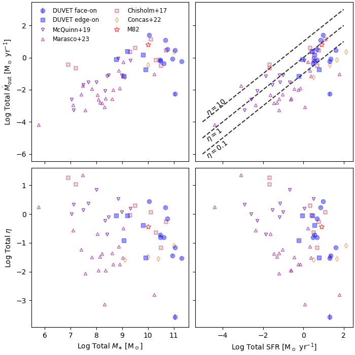
Figure 2: Summed total galaxy quantities for our 10 face-on DUVET galaxies (blue circles) and 5 DUVET edge-on galaxies (blue squares, McPherson et. al. in prep) compared with entire galaxy measurements from nearby dwarf galaxies measured in emission (down triangles, up triangles: McQuinn et al., 2019; Marasco et al., 2023, respectively), nearby star-forming galaxies measured in absorption (crosses, Chisholm et al., 2017), main-sequence star-forming galaxies at cosmic noon measured in emission (diamonds, Concas et al., 2022), and nearby starburst M 82 (red star; Greco et al., 2012; Xu et al., 2023). The panels show total galaxy measurements for mass outflow rate $\dot{M}_{\rm out}$ against total stellar mass $M_{\ast}$ (top left), and total star formation rate (top right); and the mass loading factor $\eta$ against total stellar mass $M_{\ast}$ (bottom left), and total star formation rate (bottom right). Dashed lines in the top right panel show lines of constant mass loading factor. Our DUVET targets fall within the expected scatter for total galaxy measurements. The outlier is UGC 12150, which we found had a very weak outflowing ionised gas signal.

In this section, we compare results from fitting for outflows in each spaxel to the co-located galaxy properties. We derive scaling relationships for the maximum outflow velocity, the outflow mass flux and the mass loading factor with star formation rate surface density and stellar mass surface density. A summary of these correlations is given in Table 3. We also discuss the relationship of the fraction of spaxels containing outflows with total galaxy stellar mass and global star formation rate surface density.

In Fig. 2 we compare our summed total galaxy results to literature values for total galaxy measurements of mass outflow rate, mass loading factor, total stellar mass and star formation rate. We compare our local starbursting disk galaxies to two samples of nearby dwarf galaxies (McQuinn et al., 2019; Marasco et al., 2023), a sample of nearby star-forming galaxies extending from dwarfs to Milky-Way mass galaxies (Chisholm et al., 2017), a sample of star-forming galaxies at cosmic noon (Concas et al., 2022), and the well-studied local starbursting system M 82 (e.g. Greco et al., 2012; Xu et al., 2023). We have also included results from 5 DUVET edge-on outflow systems (McPherson et al. in prep.). We note that a variety of different methods were used within the literature to obtain these values, causing scatter. For example, McQuinn et al. (2019), Marasco et al. (2023) and Concas et al. (2022) all used emission lines to trace the ionised gas outflows, where Chisholm et al. (2017) used absorption line measurements. Nevertheless, our DUVET targets fall within the range covered by the literature values. The outlier is UGC 12150, which we find has a very weak signal for outflowing ionised gas, as can be seen in the individual outflow scaling relations in Appendix B. Total galaxy outflow measurements for our 10 face-on DUVET galaxies can be found in Table 4.

$x$	$y$	$\alpha$	$\beta$	$R_{P}$	$p$-value	$R_{S}$	$p$-value
$\Sigma_{\rm SFR}$	$v_{\rm out,H\beta}$	2.44$\pm$0.01	0.19$\pm$0.01	0.44	$2\times 10^{-22}$	0.44	$1\times 10^{-22}$
$\Sigma_{\rm SFR}$	$v_{\rm out,[OIII]}$	2.48$\pm$0.01	0.10$\pm$0.02	0.16	$8\times 10^{-3}$	0.29	$6\times 10^{-7}$
$\Sigma_{\rm SFR}$	$\dot{\Sigma}_{\rm out,extcorr}$	0.57$\pm$0.03	1.25$\pm$0.03	0.86	$3\times 10^{-134}$	0.83	$3\times 10^{-116}$
$\Sigma_{\rm SFR}$	$\dot{\Sigma}_{\rm out,nocorr}$	0.27$\pm$0.04	1.20$\pm$0.04	0.76	$1\times 10^{-83}$	0.69	$3\times 10^{-63}$
$\Sigma_{\rm SFR}$	$\eta$	0.17$\pm$0.04	0.04$\pm$0.04	0.04	$0.42$	0.05	$0.26$
$\Sigma_{\ast}$	$v_{\rm out,H\beta}$	1.74$\pm$0.06	0.18$\pm$0.02	0.36	$2\times 10^{-15}$	0.35	$2\times 10^{-14}$
$\Sigma_{\ast}$	$v_{\rm out,[OIII]}$	2.04$\pm$0.10	0.11$\pm$0.03	0.18	$2\times 10^{-3}$	0.34	$5\times 10^{-9}$
$\Sigma_{\ast}$	$\dot{\Sigma}_{\rm out,nocorr}$	$-5.63\pm$0.15	1.68$\pm$0.05	0.84	$8\times 10^{-123}$	0.83	$2\times 10^{-113}$
$\Sigma_{\ast}$	$\eta$	$-2.03\pm$0.16	0.71$\pm$0.05	0.55	$3\times 10^{-}36$	0.56	$5\times 10^{-38}$

Table 3: Power law fits to the given parameters for spatially resolved data from all 10 galaxies in our sample, of the form $\log_{10}(y)=\alpha+\beta\log_{10}(x)$, using the method of orthogonal distance regression. $R_{P}$ is the Pearson correlation coefficient, with its $p$-value in the next column to the right. $R_{S}$ is the Spearman’s Rank correlation coefficient for the given correlation, with its $p$-value in the next column to the right. The subscripts ‘extcorr’ and ‘nocorr’ indicate where the outflow has been extinction corrected the same as the disk gas, or not extinction corrected, respectively.

4.1 SFR surface density and maximum outflow velocity

The kinematics of the outflow and their relationship to the SFR surface density can be used to distinguish between subgrid physical models describing the primary launching mechanism of the outflow. RC22a found a shallow relationship between the SFR surface density and the maximum outflow velocity, $v_{\rm out}\propto\Sigma_{\rm SFR}^{0.1-0.2}$, consistent with outflows driven by the energy from supernovae for IRAS 08339+6517. In this paper, we extend this analysis to nine more face-on galaxies from the DUVET sample.

We measure the star formation rate, SFR, in each spaxel using the narrow line flux from fits to the extinction corrected H$\beta$ emission line and scale them using the $L_{\rm H\alpha}/L_{\rm H\beta}$ luminosity ratio such that

$${\rm SFR}=C_{\rm H\alpha}\left(\frac{L_{\rm H\alpha}}{L_{\rm H\beta}}\right)10^{0.4A_{\rm H\beta}}L_{\rm H\beta},$$ (2)

where $C_{\rm H\alpha}=5.5335\times 10^{-42}~{}M_{\odot}~{}$yr${}^{-1}~{}($erg s${}^{-1})^{-1}$ is the scale parameter assuming a Kroupa & Weidner (2003) initial mass function (IMF; Hao et al., 2011). $L_{\rm H\alpha}/L_{\rm H\beta}=2.87$ is the luminosity ratio ($T_{e}=10^{4}$ K and Case B recombination, Osterbrock & Ferland, 2006). $A_{\rm H\beta}$ is the extinction derived from the observed H$\beta$/H$\gamma$ ratio and a Calzetti (2001) attenuation curve (see Section 3.1). $L_{\rm H\beta}$ is the observed H$\beta$ luminosity, using flux from the narrow component of the fits. This assumes that emission from the broad component is due to outflowing gas, and is not caused by star formation. RC22a found that including flux associated with outflowing gas causes an average increase in the measured $\Sigma_{\rm SFR}$ of $\sim 25\%$.

We report the total SFR for each galaxy from the H$\beta$ emission line in Column 4 of Table 1. We note that for six of the galaxies in our sample (CGCG 453-062, UGC 12150, NGC 0695, NGC 7316, IRAS 20351+2521 and KISSR 1084) the galaxy extends beyond the FOV of our KCWI pointing. The SFR that we measure is therefore a lower limit for the total SFR of these galaxies.

Star formation rate surface density, $\Sigma_{\rm SFR}$, is calculated using the spaxel size for each measurement. We find that the average spaxel within $r_{90}$ across all galaxies in the sample has a median $\log(\Sigma_{\rm SFR}[$M_⊙ yr^-1 kpc${}^{-2}])$ of -1.2 with a root-mean-square range of $\pm 0.08$ dex. Spaxels across all galaxies where we find evidence for outflows in both [OIII] $\lambda 5007$ and H$\beta$ have a median $\log(\Sigma_{\rm SFR}[$M_⊙ yr^-1 kpc${}^{-2}])$ of -0.6 with a root-mean-square range of $\pm 0.14$ dex. The typical sub-kpc region hosting outflows has, therefore, roughly half an order-of-magnitude higher $\Sigma_{\rm SFR}$ than the median across all 10 galaxies.

Following RC22a, we define the maximum outflow velocity as

$$v_{\rm out}=|v_{\rm narrow}-v_{\rm broad}|+2\sigma_{\rm broad},$$ (3)

where $v_{\rm narrow}$ and $v_{\rm broad}$ are the fitted Gaussian centres in velocity space for narrow and broad Gaussians respectively. $\sigma_{\rm broad}$ is the standard deviation of the broad Gaussian. The instrumental velocity dispersion of 0.7Å (41.9 km s^-1) is removed in quadrature. The average spaxel has a $v_{\rm out}$ measurement error of order $10-30$ km s^-1. We note that by construction of how we fit the data, this velocity should implicitly be assumed to have a negative sign, as it is the blue-shifted outflow component of the emission lines.

All of the galaxies in our sample except for IRAS 08339+6517 are brighter in H$\beta$ than in [OIII] $\lambda 5007$, with the median $\log_{10}($[OIII] $\lambda 5007/$H$\beta)$ ratio for the galaxy emission (excluding outflows) given in Table 1.

We note that CGCG 453-062 has a high inclination angle ($i\approx 54^{\circ}$), and therefore the measured outflow velocities require correction. We deproject the velocities by dividing by $\cos{i}$. For more detail on the velocity deprojection, see Appendix B. We use the deprojected velocity in the remainder of this work for CGCG 453-062. The difference in velocities after correction for galaxies with inclinations $<15^{\circ}$ is of order $\sim 5$ km s^-1, which is negligible. We, therefore, do not deproject the velocities of the rest of the galaxies as their inclination angles are below $15^{\circ}$.

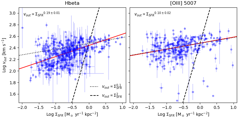
Figure 3: The maximum outflow velocity, $v_{\rm out}$, plotted against the star formation rate surface density, $\Sigma_{\rm SFR}$, for spaxels of sub-kpc resolution in 10 local starbursting disk galaxies which required a double Gaussian fit for H$\beta$ (left panel) and [OIII] $\lambda 5007$ (right panel) emission lines. For relations for individual galaxies, see Appendix B. The fit to the data is given in the top left corner and shown as a solid red line in each panel. The dashed line represents a model where outflows are primarily driven by momentum injected from young massive stars ($v_{\rm out}\propto\Sigma_{\rm SFR}^{2}$; Murray et al., 2011). The dotted line represents a model where outflows are primarily driven by energy injected from supernovae ($v_{\rm out}\propto\Sigma_{\rm SFR}^{0.1}$; Chen et al., 2010). For observations of both H$\beta$ and [OIII] $\lambda 5007$, the fitted correlation is not consistent with the momentum-driven model.

In Fig. 3 we show the results from our full sample for both the H$\beta$ and [OIII] $\lambda 5007$ emission lines, which were fit independently. For figures for individual galaxies, see Appendix B (Figures 9 and 10). In both H$\beta$ and [OIII] $\lambda 5007$ we measure the outflow velocity $v_{\rm out}$ across almost three orders of magnitude in $\Sigma_{\rm SFR}$. We find median outflow velocities of $213$ km s^-1 with a root-mean-square scatter of 234 km s^-1, and $262$ km s^-1 with a root-mean-square scatter of 279 km s^-1 for the H$\beta$ and [OIII] $\lambda 5007$ velocities respectively. We find a Pearson correlation coefficient of $R_{P}=0.44$ ($p-$value$\ll 10^{-3}$) for the relationship between $\log(\Sigma_{\rm SFR})$ and $\log(v_{\rm out})$ for H$\beta$, and $R_{P}=0.16$ ($p-$value$=0.008$) for [OIII] $\lambda 5007$.

Using the method of orthogonal distance regression we fit a relationship between $\Sigma_{\rm SFR}$ and $v_{\rm out}$ for the results from H$\beta$ and [OIII] $\lambda 5007$ separately, and find

$$v_{\rm out,H\beta}=10^{2.44\pm 0.01}\Sigma_{\rm SFR}^{0.19\pm 0.01}$$ (4)

for velocities found from fitting the H$\beta$ emission lines, and

$$v_{\rm out,OIII}=10^{2.48\pm 0.01}\Sigma_{\rm SFR}^{0.10\pm 0.02}$$ (5)

for velocities found from fitting the [OIII] $\lambda 5007$ emission lines. These fits are shown in Fig. 3 as solid red lines. We compare these to two models commonly used for the relationship between $v_{\rm out}$ and $\Sigma_{\rm SFR}$ in simulations. The dashed line shows the expected correlation if the outflows are primarily driven by the radiation pressure giving momentum to the gas surrounding young massive stars ($v_{\rm out}\propto\Sigma_{\rm SFR}^{2}$; Murray et al., 2011). The dotted line shows the expected correlation if the outflows are primarily driven by the energy injected from supernovae ($v_{\rm out}\propto\Sigma_{\rm SFR}^{0.1}$; Chen et al., 2010). We recover shallow relationships for both [OIII] $\lambda 5007$ and H$\beta$ maximum outflow velocities, which are not consistent with the model for a purely “momentum-driven” outflow.

Avery et al. (2021) fitted for ionised gas outflows using kinematically tied fits to H$\beta$, H$\alpha$, and the [OIII] $\lambda\lambda 4959,5007$, [NII] $\lambda\lambda 6548,6583$, and [SII] $\lambda\lambda 6716,6731$ doublets in radially binned star-forming galaxies with disk morphologies from the MaNGA Survey. Excluding galaxies with AGN-driven outflows, they found a shallow negative relationship of $v_{\rm out}\propto\Sigma_{\rm SFR}^{-0.07\pm 0.02}$. On the other hand, using fits to the H$\alpha$ and [NII] $\lambda\lambda 6548,6583$ emission lines, Davies et al. (2019) found a steeper relationship of $v_{\rm out}\propto\Sigma_{\rm SFR}^{0.34\pm 0.10}$ for $z\sim 2.3$ galaxies from the SINs/zC-SINF AO Survey stacked by $\Sigma_{\rm SFR}$. Our results lie between these two studies. We, however, have allowed H$\beta$ and [OIII] $\lambda 5007$ to be fit with kinematically independent fits. We note that the MaNGA galaxies cover a wide range of $\Sigma_{\rm SFR}$, but are not chosen to be starbursting as our sample of galaxies. The sample of SINs galaxies in Davies et al. (2019) has a median offset of 2$\times$ the main sequence SFR at $z=2-2.5$, and covers a similar range of $\Sigma_{\rm SFR}$ as the sample of galaxies studied here.

The galaxies in our sample do not have the same signal-to-noise in H$\beta$ as in [OIII] $\lambda 5007$ and are on average brighter in H$\beta$. The higher S/N enables us to fit the outflow component more reliably in H$\beta$. The outflow component is unresolved in [OIII] $\lambda 5007$ for the galaxies NGC 7316, CGCG 453-062 and IRAS 15229+0511. Note that excluding spaxels where we observe an outflow in only one emission line restricts the results to spaxels with ${\Sigma_{\rm SFR}>10^{-1.5}~{}M_{\odot}}$ yr^-1 kpc^-2. The fits for $v_{\rm out}-\Sigma_{\rm SFR}$ are consistent regardless of whether we restrict our data. We do find that the Pearson correlation coefficient for the outflow velocities measured in H$\beta$ increases from $R_{P}=0.44$ to $R_{P}=0.51$ ($p-$value$\ll 10^{-3}$), however, it stays the same for the [OIII] $\lambda 5007$ results at $R_{P}=0.17$ ($p-$value$=0.006$).

For those spaxels with both H$\beta$ and [OIII] broad components, the outflow velocities measured for [OIII] $\lambda 5007$ are on average $\sim 40$ km s^-1 higher than those measured for H$\beta$. The velocity is measured to be 220 km s^-1 with a root-mean-square scatter of 238 km s^-1 in H$\beta$ and 262 km s^-1 with a root-mean-square scatter of 279 km s^-1 in [OIII] $\lambda 5007$. This velocity difference is more apparent at lower $\Sigma_{\rm SFR}$. This difference could be due to systematics introduced by the absorption line around H$\beta$. Alternatively, it is plausible that [OIII] $\lambda 5007$ is associated with a higher ionisation state than H$\beta$, and this gas is intrinsically moving faster.

4.2 SFR surface density and outflow mass flux

It is expected that regions of galaxies with a higher SFR surface density will drive a higher mass outflow rate, $\dot{M}_{\rm out}$, which has been observed in resolved observations of one target (RC22b). The mass outflow rate is defined as

$$\dot{M}_{\rm out}=\frac{1.36m_{\rm H}}{\gamma_{\rm H\beta}n_{e}}\left(\frac{v_{\rm out}}{R_{\rm out}}\right)L_{\rm H\beta,broad}10^{0.4A_{\rm H\beta}},$$ (6)

where $m_{\rm H}$ is the atomic mass of hydrogen. $\gamma_{\rm H\beta}$ is the H$\beta$ emissivity for case B recombination with assumed electron temperature ${T_{e}=10^{4}}$ K ($\gamma_{\rm H\beta}=1.24\times 10^{-25}$ erg cm³ s^-1; Osterbrock & Ferland, 2006). $n_{e}$ is the local electron density in the outflow, where we assume $n_{e}=100$ cm^-3 (RC22b). $v_{\rm out}$ is the maximum outflow velocity found from fitting the emission lines, here we use the $v_{\rm out}$ from H$\beta$. $R_{\rm out}$ is the radial extent of the outflow, where we assume $R_{\rm out}=0.5$ kpc. $L_{\rm H\beta}$ is the H$\beta$ luminosity from the fitted broad Gaussian component. Finally, $A_{\rm H\beta}$ is the extinction derived from the observed H$\beta$/H$\gamma$ ratio for the narrow line component and a Calzetti (2001) attenuation curve (see Section 3.1), which is discussed further below. For discussion of the motivation and likely systematic uncertainty on $R_{\rm out}$ see RC22a, and on $\gamma_{\rm H\beta}$ and $n_{e}$ see RC22b.

The outflow mass flux is the mass outflow rate divided by the surface area of the measurement $\dot{\Sigma}_{\rm out}=\dot{M}_{\rm out}/{\rm Area}$. The outflow mass flux is a more useful measurement in resolved outflow studies than the outflow mass rate, and can be compared to results from simulations, especially high-resolution box simulations (e.g. Kim & Ostriker, 2017; Rathjen et al., 2023).

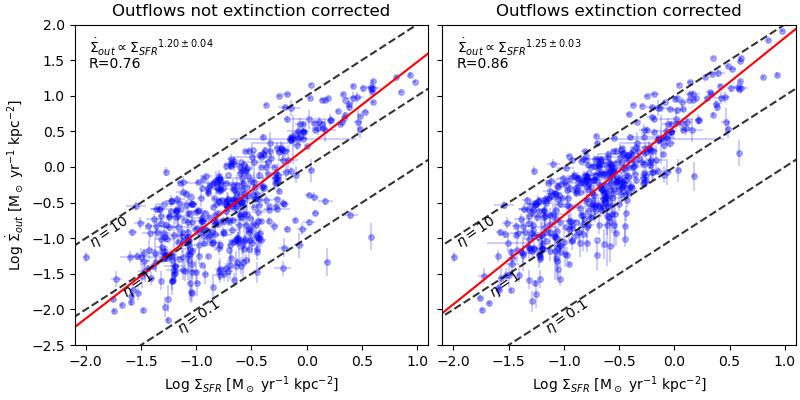
Figure 4: The ionised gas outflow mass flux, $\dot{\Sigma}_{\rm out}$, compared to the SFR surface density, $\Sigma_{\rm SFR}$, for sub-kpc resolution spaxels in local starbursting disk galaxies with evidence for outflow components. We fit a relationship between the two quantities using the method of orthogonal distance regression, which returns a nonlinear correlation, given with the Pearson correlation coefficient in the top left corner and plotted as a red solid line. Dashed black lines show constant mass loading factors. The left panel shows no extinction correction on the outflow. The right panel shows $\dot{\Sigma}_{\rm out}$ with the same extinction correction applied as for gas in the disk.

We do not have sufficient S/N on H$\gamma$ to resolve the outflow component, and then determine an extinction correction for the outflow. We therefore compare our results assuming the same extinction correction that we applied for the disk to the outflow, to our results when assuming no extinction in the outflow. The assumptions of no extinction or the same extinction as in the disk represent the extremes, where the actual value likely lies in between, and may vary from galaxy to galaxy. We note that it is often an implicit assumption that $\dot{M}_{\rm out}$ includes the same extinction as the ISM, for example in calculating $\eta\propto F_{\rm broad}/F_{\rm narrow}$. While dust certainly exists in outflows (e.g. Engelbracht et al., 2006; Roussel et al., 2010), the extinction is likely not as high as in the midplane of the galaxy. Xu et al. (2022) approximated the total dust extinction using absorption-line outflows of CLASSY galaxies and found that most of the dust responsible for extinction resides within the static ISM.

In the right-hand panel of Fig. 4 we plot the extinction-corrected outflow mass flux against the SFR surface density for all galaxies in our sample. We measure ${\dot{\Sigma}_{\rm out}\sim 0.01~{}M_{\odot}}$ yr^-1 kpc^-2 to $\sim 100~{}M_{\odot}$ yr^-1 kpc^-2 over three orders of magnitude in $\Sigma_{\rm SFR}$. The median $\log(\dot{\Sigma}_{\rm out}[M_{\odot}$ yr^-1 kpc${}^{-2}])$ for our sample was -0.25 with a root-mean-square of $\pm 0.83$ dex. We find a Pearson correlation coefficient of $R_{P}=0.86$ ($p-$value$\ll 10^{-3}$) for $\log\dot{\Sigma}_{\rm out}-\log\Sigma_{\rm SFR}$. Due to the large range of error bars in outflow mass flux, fitting the data would be biased towards the high S/N points at high SFR surface density. We, therefore, constrain the error bars to have a minimum uncertainty of 0.15 dex in $\dot{\Sigma}_{\rm out}$ for the fit. Fitting the data using the method of orthogonal distance regression, we find a superlinear relationship of

$$\dot{\Sigma}_{\rm out}=10^{0.57\pm 0.03}~{}\Sigma_{\rm SFR}^{1.25\pm 0.03}.$$ (7)

We show this fit as a red line in the right-hand panel of Fig. 4. This is slightly steeper than the relationship found in RC22b ($\dot{\Sigma}_{\rm out}\propto\Sigma_{\rm SFR}^{1.06\pm 0.10}$). When the errorbars are used without modification, we find a steeper correlation $\dot{\Sigma}_{\rm out}\propto\Sigma_{\rm SFR}^{1.33\pm 0.03}$, which is consistent with the relationship found with unconstrained errorbars in RC22b. We observe values of $\dot{\Sigma}_{\rm out}$ an order of magnitude lower than found in RC22b, and these low S/N results may weight the fit towards low $\dot{\Sigma}_{\rm out}$ values when the error bars are unconstrained.

In the left panel of Fig. 4, we show the same relationship if we assume no extinction in the outflow. With no extinction correction, we find a median $\log(\dot{\Sigma}_{\rm out}[M_{\odot}$ yr^-1 kpc${}^{-2}])$ of -0.57 with a root-mean-square of $\pm 0.50$ dex. We also find a slightly shallower relationship between the mass outflow flux and the SFR surface density, such that $\dot{\Sigma}_{\rm out}\propto\Sigma_{\rm SFR}^{1.20\pm 0.04}$. This is consistent with the relationship found in RC22b within uncertainties. If we do not apply an extinction correction to the outflows in the same manner as we do to the SFR, we find mass loading factors a factor of 3 lower, with a median mass loading factor of 1.55 with a root-mean-square scatter of 3.24. We use the non-extinction corrected values of $\dot{\Sigma}_{\rm out}$ for the remainder of the paper.

In Appendix B we show the same relationship as Fig. 4, but plotting each galaxy in our sample individually. We find that each galaxy has a trend of increasing outflow mass flux with increasing SFR surface density. We interpret this to suggest that the important change from galaxy to galaxy is the overall degree of star formation, yet roughly the same local relationship between $\dot{\Sigma}_{\rm out}$ and $\Sigma_{\rm SFR}$ remains.

There is a wide range of results in the literature for the galaxy-integrated relationship between the total outflow mass rate and SFR. Fluetsch et al. (2019) found $\dot{M}_{\rm out}\propto$ SFR^1.19±0.06 for molecular gas outflows in local star-forming galaxies. Avery et al. (2021) found a shallower relationship, $\dot{M}_{\rm out}\propto{\rm SFR}^{0.84\pm 0.08}$, for ionised gas outflows using star-forming galaxies from MaNGA, excluding AGN from their sample. In a follow-up paper of the same galaxies, Avery et al. (2022) found a relationship of $\dot{M}_{\rm out}\propto{\rm SFR}^{0.74\pm 0.2}$ for the neutral gas outflows. For a sample of dwarf starbursting galaxies from the DWALIN survey, Marasco et al. (2023) found an even shallower result, $\dot{M}_{\rm out}\propto$ SFR^0.4. However, we caution that these galaxy-averaged measurements almost certainly include regions that do not drive an outflow but do contribute to the total SFR.

Using magnetohydrodynamic box simulations of the ISM and star formation-driven outflows with the SILCC framework, Rathjen et al. (2023) found $\dot{\Sigma}_{\rm out}\propto\Sigma_{\rm SFR}^{0.81\pm 0.12}$ for the total gas outflow mass flux. They suggested that more massive galaxies with higher $\Sigma_{\rm SFR}$ have more difficulty driving outflows from their larger potential wells, leading to a sublinear correlation. Considering only the warm ionised gas, Rathjen et al. (2023) found a steeper relationship of $\dot{\Sigma}_{\rm out}\propto\Sigma_{\rm SFR}^{1.40\pm 0.24}$. This is steeper than the slope which we fit in Fig. 4 (see also Eq. 7). However, our galaxies cover a range of SFR surface densities that extends at least an order of magnitude beyond the maximum SFR surface density ($\Sigma_{\rm SFR}\sim 0.2~{}M_{\odot}$ yr^-1 kpc^-2) modelled by Rathjen et al. (2023), and so a complete comparison is difficult. It is possible that the less dense ionised gas can be accelerated more efficiently than the cold phases of gas, leading to a steeper correlation. This difference could explain the shallower slope which Avery et al. (2022) observed for their molecular gas outflows than we find for ionised gas outflows, although Avery et al. (2022) found agreement at the $1\sigma$ level between their observations of ionised and neutral gas outflows.

4.3 Mass loading factor

The mass loading factor describes the efficiency of a galaxy in driving outflows. The resolved mass loading factor is the ratio between the mass outflow flux and the star formation rate surface density

$$\eta=\frac{\dot{\Sigma}_{\rm out}}{\Sigma_{\rm SFR}}.$$ (8)

The mass loading factor relates the rate of gas leaving a region of the galaxy to the underlying star formation driving the outflow. Regions of a galaxy with a mass loading factor greater than 1 are driving more gas out of the galaxy than they are turning into stars.

In Fig. 4 we show lines of constant mass loading factor as diagonal dashed black lines. When we consider all galaxies in our sample, we find that for the majority of spaxels we measure an ionised gas mass loading factor between 0.1 and 10. We find a median mass loading factor of 1.55 with a root-mean-square scatter of 3.24. We did not find a statistically significant correlation between the mass loading factor and the SFR surface density, with a Pearson correlation value of $R_{P}=0.04$ ($p$-value$=0.42$) between $\log(\eta)$ and $\log(\Sigma_{\rm SFR})$. This is expected, due to the almost linear correlation we find between the mass outflow flux and the SFR surface density. Our results suggest that in the majority of the regions where we observe an outflow, the star formation is efficiently coupled to the gas to drive the outflow.

Outflows are by nature multiphase. When calculating the mass loading factor we, therefore, need to take into account the total mass budget of the outflow. Fluetsch et al. (2019) found roughly comparable mass outflow rates from ionised and molecular gas observations of outflows in four galaxies with a similar specific star formation rates, sSFR$=$SFR/$M_{*}$, to the galaxies in our sample. This would imply a total mass loading factor for our galaxies of order $\eta\sim 2-20$. In contrast to this, Fluetsch et al. (2021) found that for local ULIRGs, the mass of ionised gas in the galaxy wind is a very small fraction ($<5\%$) of the total mass outflow, with neutral gas making up $\sim 10\%$ and molecular gas up to $\sim 95\%$ of the outflowing mass. Similarly, Roberts-Borsani et al. (2020) found that ions contribute $<1\%$ of the mass to the total outflowing gas mass. Following these studies, the total mass loading factor for the galaxies we observe here could be anywhere from $\eta\sim 10-100$ or even greater.

Avery et al. (2022) compared the analysis of ionised gas outflows in the MaNGA galaxies from Avery et al. (2021) to observations of neutral gas outflows studied using the Na I D absorption feature. Avery et al. (2022) accounted for the dust extinction in the outflow separately from that within the ISM of the galaxy and found that this increased the fraction of the total gas mass measured in ionised gas. Even with this correction, the ionised gas phase mass they measured remained $\sim 1.2$ dex lower than the neutral gas phase mass. They found an average neutral gas mass loading factor of order unity for non-AGN MaNGA galaxies within a similar mass range to our galaxies. If our galaxies follow a similar trend, then we could expect to observe neutral gas mass loading factors of $\sim 10-100$, which is far higher than the neutral gas mass loading factors that Avery et al. (2022) found. Alternatively, if we expect the galaxies in our sample to have similar neutral gas mass loading factors to those found by Avery et al. (2022), then it is possible that neutral gas observations of the galaxies in our sample would find roughly comparable ionised and neutral gas mass loading factors. This would then be similar to the results from Fluetsch et al. (2019).

However, we urge caution when comparing observational results between resolved studies such as this one and studies utilising stacked spectra or total galaxy measurements such as Avery et al. (2022) and Fluetsch et al. (2019). Normalising the mass outflow rate by the star formation rate may include star formation from regions of the galaxy that do not drive an outflow in non-resolved studies. This can result in an artificially low mass loading factor for some observations.

Moreover, observations of the mass loading factor inherently include a large number of assumptions about the geometry and electron density of the outflow. These assumptions can vary dramatically between studies and can have a large impact on the results. For example RC22b found that increasing the assumed electron density from $n_{e}=100$ cm^-1 to $n_{e}=300$ cm^-1 decreased the mass loading factor by $\sim 0.5$ dex. The electron density within the disk has been observed to depend on the local SFR surface density (e.g. Kaasinen et al., 2017; Davies et al., 2021). If the electron density of the outflow also depends on the SFR surface density such that the electron density decreases for brighter outflows, this would steepen the correlation between the mass loading factor and SFR surface density, bringing our result closer to predictions from simulations (e.g. Kim et al., 2020; Pandya et al., 2021). Alternatively RC22b also found that increasing the assumed outflow radius from $R_{\rm out}=0.5$ kpc to $R_{\rm out}=20$ kpc decreased the mass loading factor by $\sim 1.5$ dex. If the $R_{\rm out}$ increases for outflows driven by stronger star formation, this might offset a change in the electron density. It is therefore difficult to definitively say how our assumptions impact our results. High-resolution studies of outflows from edge-on galaxies such as the MUSE/VLT GECKOS Large Program are likely to make progress on understanding these systematics (Elliot in prep).

In addition, while we expect that there should be an order of magnitude more molecular gas than ionised gas in the total outflow mass budget, regions of the galaxy with higher SFR surface densities may well be ionising more gas, increasing the fraction of ionised gas in the outflow. Simply assuming the same ratio of ionised-to-molecular gas in the outflow for all SFR surface densities may therefore lead us to overestimate the total mass loading factor. For example, in the MHD stratified galaxy patch simulation SILCC, Rathjen et al. (2023) found a steeper relationship between the warm and ionised outflow mass rate and the SFR surface density than between the total outflow mass rate and the SFR surface density. This suggests that for regions with higher SFR surface densities, ionised gas may make up a larger fraction of the total outflowing mass.

Simulations use the relationship between the mass loading factor and the SFR surface density to test the driving mechanisms of outflows. A number of simulations predict a negative relationship of $\eta_{\rm ion}$ with SFR surface density (Fielding et al., 2017; Li et al., 2017; Kim et al., 2020; Pandya et al., 2021). With our sample of galaxies, however, we find a very shallow positive relationship between the mass loading factor and the SFR surface density. We now compare the mass loading factor values from the simulations to those measured in our observations. Using the FIRE suite of cosmological zoom-in simulations, Anglés-Alcázar et al. (2017) found total gas mass loading factors of $\eta\sim 2$ for galaxies in a similar galaxy mass range to our sample. From the updated FIRE-2 simulations, Pandya et al. (2021) found that the warm ($10^{3}~{}{\rm K}<T<10^{5}$ K) gas represents less than 10% of the total mass loading for galaxies with a similar stellar mass to our sample. For $\Sigma_{\rm SFR}\sim 0.1-10~{}M_{\odot}$ yr^-1 kpc^-2 they find warm gas mass loading factors ranging from $\eta\sim 0.04-10$. These values are within the range of the mass loading factors we find for the ionised gas phase observations in our galaxies. Using the SMAUG-TIGRESS simulations, Kim et al. (2020) similarly found mass loading factors for the cool ($T\sim 10^{4}$ K) gas of $\eta\sim 0.2-10$ for $\Sigma_{\rm SFR}\sim 0.1-1~{}M_{\odot}$ yr^-1 kpc^-2. These values are consistent with the values we observe in our galaxies at a similar SFR surface density.

We note that we are not comparing apples with apples. Kim et al. (2020) simulate solar neighbourhood-like conditions and do not reach the high $\Sigma_{\rm SFR}$ environments of some regions of our targets. In addition, Pandya et al. (2021) calculate total values of $\eta$ and SFR surface density for entire galaxy haloes, while we calculate these values for resolved regions. While our extended sample covers a larger range of SFR surface densities than RC22b, our results are however still within the scatter of results returned for the warm ionised gas by Pandya et al. (2021).

4.4 Stellar mass surface density

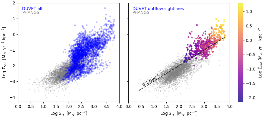
Figure 5: The so-called “resolved main-sequence” for DUVET galaxies. The left panel shows all spaxels within $r_{90}$. The right panel shows the same region, but only for those spaxels with outflows. Grey points are kiloparsec-scale measurements from the PHANGS sample. The line is an ad hoc seperation showing that outflows become more common for $\Sigma_{\rm SFR}/\Sigma_{\ast}>0.1$ Gyr^-1. Outflow points are coloured by outflow mass flux.

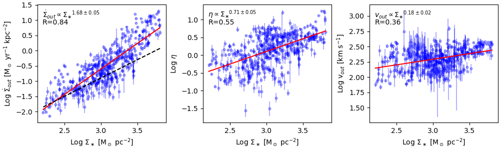
Figure 6: The relationship between the resolved stellar mass surface density and the outflow mass flux (left), the mass loading factor (middle), and the outflow velocity (right). We fit a relationship between the two quantities for each panel using the method of orthogonal distance regression. The resulting nonlinear correlations are given with the Pearson correlation coefficient in the top left corner of each panel, and are plotted as solid red lines. In the left panel, the dashed black line shows $\dot{\Sigma}_{\rm out}\propto\Sigma_{\ast}^{1.2}$, which would be the case if the $\dot{\Sigma}_{\rm out}-\Sigma_{\ast}$ relation followed the $\dot{\Sigma}_{\rm out}-\Sigma_{\rm SFR}$ relation.

In Fig. 5 we show the so-called “resolved main-sequence” relationship between $\Sigma_{\rm SFR}$ and $\Sigma_{\ast}$ for DUVET targets in this work. We derive stellar masses using 2MASS H-band observations, which are available for all of our sources. The 2MASS data is convolved and resampled to match the DUVET KCWI images. Our galaxies are selected to be starbursts, so to convert to stellar mass we assume an LMC mass-to-light ($M/L$) ratio (Eskew et al., 2012) of $M/L_{H}=0.11$ by scaling the 3.6 $\mu$m M/L to H-band, and the Salpeter (1955) IMF to a Kroupa & Weidner (2003) IMF. We note that we tested the Meidt et al. (2012) method using Spitzer 3.6 $\mu$m and 4.5 $\mu$m images, and determined that Spitzer 3.6 $\mu$m images in our sample are likely to be very strongly affected by 3.3 $\mu$m PAH feature, which varied significantly across our targets. We, therefore, opted not to use methods like Meidt et al. (2012) as the PAH feature introduced extra systematics to the conversion to stellar mass. In Fig. 5 we compare our $\Sigma_{\rm SFR}$ and $\Sigma_{\ast}$ to those of the PHANGS sample (Sun et al., 2023), measured with comparable resolution, and find that for regions of DUVET galaxies with $\Sigma_{\rm SFR}$ that is similar to values of PHANGS targets the $\Sigma_{\ast}$ is likewise comparable.

The DUVET sample is selected to have global SFR and M_∗ that is nominally at least 5$\times$ higher than the star-forming main sequence, and this is reflected in Fig. 5. In the left panel of the figure, we show all lines of sight, the majority of which have higher $\Sigma_{\rm SFR}/\Sigma_{\ast}$ than PHANGS galaxies, which are more representative of the resolved star-forming main sequence. Overall, the DUVET targets have a spread in $\Sigma_{\rm SFR}/\Sigma_{\ast}$ that begins at the resolved main sequence and skews upwards.

In the right panel of Fig. 5 we show only those lines of sight in which our automatic detection method identifies outflows. Nearly 100% of the lines of sight containing outflows are above the main sequence. We also plot a line corresponding to $\Sigma_{\rm SFR}/\Sigma_{\ast}=0.1$ Gyr^-1. Outflows are very rare below this specific star formation rate, at any value of $\Sigma_{\ast}$. We find that below $\Sigma_{\rm SFR}/\Sigma_{\ast}=0.1$ Gyr^-1 only 9% of all spaxels are determined to have outflows, and above this value 20% do have outflows. Out of all the spaxels with outflows, 78% have $\Sigma_{\rm SFR}/\Sigma_{\ast}>0.1$ Gyr^-1.

A large number of studies conclude that outflows are more common at higher specific SFR (Förster Schreiber et al., 2019; Avery et al., 2021; Roberts-Borsani et al., 2020; Veilleux et al., 2020; Chen et al., 2010; Rubin et al., 2014, e.g.). Our result in Fig. 5 shows that this extends down to sub-kpc scales. More specifically, Förster Schreiber et al. (2019) showed that $z\approx 2$ KMOS3D galaxies that are above the main sequence are much more likely to host outflows, similar to our result. There are both theoretical and observational arguments (Murray et al., 2011; Heckman et al., 2002) that a minimum $\Sigma_{\rm SFR}\gtrsim 0.1$ M_⊙ yr^-1 kpc^-2 is needed to drive observable outflows. While we do find outflows become less common below this threshold, it is clear from Figures 4 and 5 that they are still present and seem to extend the correlations of higher $\Sigma_{\rm SFR}$ winds. We find that 28% of the spaxels we observe to contain outflows fall below this threshold. It is possible that any threshold value in $\Sigma_{\rm SFR}$ is likely to increase at higher $\Sigma_{\ast}$. This can be understood by a simple argument in which the higher $\Sigma_{\ast}$ exerts a greater gravitational force on the outflow gas. The gas may require more energy, from higher $\Sigma_{\rm SFR}$, to escape the local potential. This would be consistent with where we find outflows in the DUVET targets.

In Fig. 6 we compare $\Sigma_{\ast}$ for individual spaxels to the outflow properties ($\dot{\Sigma}_{\rm out}$, $\eta$ and $v_{\rm out}$). All three show positive correlations. The correlation of $\dot{\Sigma}_{\rm out}-\Sigma_{\ast}$ is similarly strong as that of $\dot{\Sigma}_{\rm out}-\Sigma_{\rm SFR}$, with a Pearson correlation coefficient $R_{P}=0.84$ ($p-$value$\ll 10^{-3}$). We find, however, that the powerlaw of this relationship is steeper, such that $\dot{\Sigma}_{\rm out}\propto\Sigma_{\ast}^{1.68\pm 0.05}$, where the powerlaw index scaling with $\Sigma_{\rm SFR}$ is closer to $\sim 1.2$. Similarly, the correlation of $\eta-\Sigma_{\ast}$ is steeper than $\eta-\Sigma_{\rm SFR}$, such that $\eta\propto\Sigma_{\ast}^{0.71\pm 0.05}$, with a Pearson correlation coefficient of $R_{P}=0.55$ ($p-$value$\ll 10^{-3}$). The powerlaw index scaling for $\eta-\Sigma_{\rm SFR}$ is closer to zero. The correlation of $v_{\rm out}$ with $\Sigma_{\ast}$ is shallow and similar to that with $\Sigma_{\rm SFR}$.

We do not know why the correlation of $\dot{\Sigma}_{\rm out}$ with $\Sigma_{\ast}$ should be so steep. For spaxels with outflows the correlation of $\Sigma_{\rm SFR}$ with $\Sigma_{\ast}$ is roughly consistent with linear. Therefore, if we assume that $\dot{\Sigma}_{\rm out}-\Sigma_{\ast}$ is a secondary correlation between $\dot{\Sigma}_{\rm out}$ and $\Sigma_{\rm SFR}$ then we would expect the same powerlaw.

We note that the steep powerlaw of $\dot{\Sigma}_{\rm out}\propto\Sigma_{*}^{1.68}$ may be a relic of systematic uncertainties. We assumed a constant $M/L$ across our sample. However, if this changes due to the local stellar populations or position in the galaxy, then this could impact the powerlaw. In this case, however, the most likely scenario would be that higher $\Sigma_{\rm SFR}$ would have younger stellar populations and thus lower $M/L$. This would steepen the relationship.

There are also physical arguments for a steeper relationship with $\Sigma_{\ast}$. For example, higher $\Sigma_{\ast}$ implies a stronger local gravitational potential. In principle, this requires outflows to be stronger for them to overcome the local gravity, and be observed in our sample. Secondly, as the highest $\Sigma_{\ast}$ spaxels are preferentially in the galaxy center, it may be that gas is preferentially built up in these regions and thus able to drive stronger winds.

4.5 Outflow covering fraction

The covering fraction of outflows is defined by the total fraction of starlight that is covered by outflowing gas. This quantity is necessary when calculating the mass-outflow rate for entire galaxy outflow measurements (e.g. at higher redshift; Rubin et al., 2014; Davies et al., 2019) or for edge-on galaxy outflow measurements. In absorption line measurements it is typically inferred from the depth of the absorption line. Our resolved outflow measurements allow us to measure this directly via geometry. See McPherson et al. (2023) for a similar calculation in an edge-on outflow galaxy.

Here we calculate the covering fraction as $f_{\rm cov}\equiv N_{\rm outflow}/N_{\rm total}$, where $N_{\rm outflow}$ and $N_{\rm total}$ are, respectively, the number of spaxels with an outflow and the total number of spaxels. We calculate this for each galaxy within the 90% starlight radius ($r_{90}$) and half-light radius ($r_{50}$). In Fig. 7 we compare $f_{\rm cov}$ within $r_{50}$ and $r_{90}$ to the total galaxy stellar mass, and the median SFR surface density within $r_{50}$ and $r_{90}$ for outflows detected in H$\beta$.

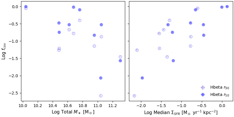
Figure 7: The fraction of spaxels with outflows detected in in H$\beta$ within $r_{50}$ (coloured points) and $r_{90}$ (open points) for each galaxy is plotted against the total stellar mass (left panel), and the median SFR surface density (right panel) of the galaxies. We find the strongest correlation is a dependence of the covering fraction on the median SFR surface density.

Across our galaxy sample, we find a trend of decreasing covering fraction with increasing stellar mass, shown in the left panel of Fig. 7. The correlation between the covering fraction and the total galaxy stellar mass has a Pearson correlation coefficient of $R_{P}=-0.60$ ($p-$value$=0.005$) for the relationship $\log(f_{\rm cov})-\log(M_{*})$. For galaxies with $\log M_{*}[M_{\odot}]=10.7-11.5$ we find a median covering fraction of 15% within $r_{50}$. For the lower mass galaxies in the sample ($\log M_{*}[M_{\odot}]=10-10.7$), we find the covering fraction increases to 34%. The decrease in the fraction of outflow spaxels with increasing stellar mass seems connected to our result in Fig. 5, where individual spaxels with higher $\Sigma_{\ast}$ require higher $\Sigma_{\rm SFR}$ to be observed with an outflow. Similarly, this can be understood given that galaxies with a higher stellar mass have a larger gravitational potential well, making it harder to accelerate outflows to the velocities necessary to leave the disk.

The right panel of Fig. 7 shows the relationship between the covering fraction and the median value of the SFR surface density. This is calculated within $r_{50}$ to compare to the covering fraction within $r_{50}$, and similarly within $r_{90}$ to compare to the covering fraction within $r_{90}$. We find an overall trend of increasing covering fraction with increasing median SFR surface density. This trend has a higher statistical significance, with a Pearson correlation coefficient of $R_{P}=0.76$ ($p-$value$=0.0001$) for $\log(f_{\rm cov})-\log(\Sigma_{\rm SFR,median})$. Given the local correlations between outflow properties and $\Sigma_{\rm SFR}$, this trend seems straightforward to understand. If the typical $\Sigma_{\rm SFR}$ in a galaxy is larger then this galaxy will have a larger area in which outflows are present.

We also test the correlation of the covering fraction with stellar mass and median SFR surface density for our results using [OIII] $\lambda 5007$. We find the same correlation with stellar mass (Pearson correlation coefficent $R_{P}=-0.60$, $p-$value$=0.02$), and a slightly less strong correlation with median SFR surface density (Pearson correlation coefficent $R_{P}=0.51$, $p-$value$=0.05$). However, overall fewer spaxels contain outflows.

Additionally, we also test the covering fraction out to $r_{90}$. We find that the fraction of spaxels with outflows decreases between $r_{50}$ and $r_{90}$ by a median of 0.33 dex for H$\beta$ and 0.29 dex for [OIII] $\lambda 5007$, suggesting that the majority of outflows are centrally located, although not all outflows are launched from the centre of the galaxies. This is similar to results from Avery et al. (2022) for the MaNGA galaxies, who found that most neutral gas outflows are concentrated centrally within $\sim 0.25~{}R_{e}$.

Using absorption line measurements for 105 galaxies at $0.3<z<1.4$, Rubin et al. (2014) found a median covering fraction of $\sim 0.65$ for both the Mg II and Fe II absorption lines. This is far higher than what we find using emission lines to trace the ionised gas. However, absorption line measurements are sensitive to gas clouds at any distance along the line-of-sight to the host galaxy. It is likely that they are able to probe outflowing gas that has reached further from the galaxy than our emission line measurements, which probe the base of the outflow. Their higher covering fractions could, therefore, be caused by outflowing gas which has either been driven by underlying star formation which is no longer observable, or has expanded further across the face of the galaxy due to the outflow opening angle.

In addition, Rubin et al. (2014) found covering fractions $\gtrsim 0.5$ in 75% of the absorption lines where they also measured equivalent widths for the outflow component EW${}^{16\%}_{\rm flow}>0.2$ Å. They found a dependence of the outflow equivalent width on the covering fraction. They also found that the outflow equivalent width was correlated with the SFR, such that galaxies with a higher SFR launch more material with a larger range of velocities. Prusinski et al. (2021) also found a relationship between the equivalent width and the covering fraction such that galaxies with more intense star formation drive outflows with a higher covering fraction and a wider range of velocities. These studies are in agreement with our result that galaxies with a higher SFR surface density have a higher covering fraction.

5 Conclusions

In this paper we present sub-kpc spatially-resolved scaling relations for star formation-driven outflows and properties of their host galaxies on 10 galaxies from the DUVET sample. We fit multi-component Gaussians to the H$\beta$ and [OIII] $\lambda 5007$ emission lines in 10 near-to-face-on galaxies. We find the following main results.

1. We find shallow relationships of the maximum outflow velocity with the SFR surface density for both H$\beta$ ($v_{\rm out,H\beta}\propto\Sigma_{\rm SFR}^{0.19\pm 0.01}$) and [OIII] $\lambda 5007$ ($v_{\rm out,OIII}\propto\Sigma_{\rm SFR}^{0.10\pm 0.02}$). These fitted relationships are not consistent with models of outflows that are dominated by momentum-driven winds ($v_{\rm out}\propto\Sigma_{\rm SFR}^{2}$; Murray et al., 2011), and suggests supernovae as the dominant energy source driving the wind (e.g. Kim et al., 2020).

2. We fit a nonlinear relationship between the mass outflow flux and the SFR surface density such that $\dot{\Sigma}_{\rm out}\propto\Sigma_{\rm SFR}^{1.20\pm 0.04}$.

3. We find ionised gas mass loading factors between $\sim 0.1$ and $\sim 10$, and approximate a total median mass loading factor of $\sim 2-100$. We fit an almost flat relationship between the mass loading factor and the SFR surface density which has no significant correlation.

4. We make a direct comparison of outflow properties to the stellar mass surface density and specific star formation rate. Outflows are much more common for $\Sigma_{\rm SFR}/\Sigma_{\ast}\gtrsim 0.1$ Gyr^-1. We note that outflows are observed to lower $\Sigma_{\rm SFR}$ than previous threshold values. We also find strong, positive correlations between outflow properties and co-located $\Sigma_{\ast}$. In particular we find that outflow mass flux correlates with the stellar mass surface density such that $\dot{\Sigma}_{\rm out}\propto\Sigma_{\ast}^{1.68\pm 0.05}$.

5. We compare the fraction of spaxels where we find evidence for outflows within $r_{50}$ and $r_{90}$ to the total galaxy stellar mass, and the median galaxy SFR surface density within $r_{50}$ and within $r_{90}$. We find a negative correlation with stellar mass and a positive relationship with median SFR surface density. This is consistent with the picture where galaxies of higher mass have a larger gravitational potential well, and require more concentrated star formation to drive gas out of the disk.

The observed scaling relations of outflow properties with the SFR surface density suggest that outflows are primarily driven by energy from supernovae. If supernovae are primarily driving the outflows, then the winds linearly correlate to the SFR surface density. We should therefore expect that if you change the spatial distribution of the starburst then the outflow distribution will follow. Our covering fraction results are consistent with this picture.

This has multiple implications. Firstly, galaxies at higher redshift may have a different outflow structure than local starburst galaxies (e.g. M 82 and NGC 253). While local starbursts are typically concentrated in the central kiloparsec of the galaxy, galaxies at higher redshift have clumpier morphologies, which may affect the structure of the outflowing gas. Secondly, simulations suggest that outflows that have greater covering fractions may have different energetics. Schneider et al. (2018) found that altering the geometry of the simulated galaxy wind enables more gas cooling within the outflow.

Our observation that outflows are more common in higher specific SFR regions of galaxies seems straightforward to understand. Higher $\Sigma_{\rm SFR}$ provides more energy to the wind, and higher $\Sigma_{\ast}$ creates more gravity reducing the outflow’s ability to break out of the disk. Therefore as we increase the $\Sigma_{\ast}$ the $\Sigma_{SFR}$ required to drive an outflow must also increase. We note that this boundary, $\Sigma_{\rm SFR}/\Sigma_{\ast}\sim 0.1$ Gyr^-1 is only a factor of $\sim$2$\times$ above the resolved main-sequence for similar regions (Sánchez et al., 2021). It may be that a combination of thresholds in both SFR surface density and specific SFR is needed to predict the location of outflows.

We do not have a direct theoretical prediction for the steep scaling relationship of $\dot{\Sigma}_{\rm out}\propto\Sigma_{\ast}^{1.68\pm 0.05}$. We know that $\Sigma_{\rm SFR}$ correlates with both outflow properties and stellar mass surface density. This may generate a secondary correlation between the outflow and the stellar mass surface density, and the steep scaling could simply be a result of uncertainties. Alternatively, it may be that the higher stellar mass demands stronger outflows for gas to break out of the plane of the disk and be observed as an outflow. More work relating the resolved stellar mass properties, both stellar populations and kinematics, with the feedback and gas properties is clearly warranted to understand this correlation.

There are a number of limitations to our analysis. We must make many assumptions about the outflow geometry and the electron density to calculate some of these properties, particularly the mass outflow flux and the mass loading factor. Future work obtaining resolved observations of outflows capable of testing these assumptions is underway (Elliot et al. in prep) with the GECKOS MUSE LP (van de Sande et al., 2023). It is also unclear whether the constant mass loading we observe in our sample here persists in lower SFR surface density environments. The mass that the star formation is able to lift out of the galaxy may begin to decline more rapidly as the star formation activity decreases.

More work adding observational constraints to the total mass loading considering the multi-phase nature of outflows and its dependence on SFR surface density and geometry is needed. In the future, with new facilities such as the ELT, we will be able to test the contribution of underlying stellar population parameters on star formation-driven feedback in starbursting galaxies on the scale of stellar clusters.

Data Availability

Data underlying this article from the DUVET survey will be shared on reasonable request to the PI, Deanne Fisher, at dfisher@swin.edu.au. All other data used within this article is archival and available publicly.

Appendix A Choosing the $\delta_{\rm BIC}$ threshold

The typical literature value used for the BIC threshold is $\delta_{\rm BIC}=-10$ (Kass & Raftery, 1995; Swinbank et al., 2019; Avery et al., 2021). However, this threshold is based on the assumption that the model errors are independent and distributed according to a normal distribution. Emission lines in typical spiral galaxies have been shown to be better fit by multiple Gaussian components (Ho et al., 2014). Observations of singular H II regions also find emission lines require multiple Gaussian components (Rozas et al., 2007) or a Voigt profile (Keto et al., 2008; Galván-Madrid et al., 2012). Our data has extremely high signal-to-noise. We select only spaxels that have a median signal-to-noise per wavelength channel of $\gtrsim 10$, implying a peak signal-to-noise of 100-200 across many of the emission lines. This is sufficiently high to identify any fluctuations away from a Gaussian shape in the galaxy emission, even with the limited spectral resolution. In addition, the models available for continuum subtraction are imperfect representations of young, starburst populations, and residuals from this process may be mistaken for a low-flux broad component if a lenient $\delta_{\rm BIC}$ is used. In RC22a we found that using the typically adopted threshold value of $\delta_{\rm BIC}$ results in all spaxels requiring multiple Gaussian component models, even those spaxels in which a by-eye examination favours only a single Gaussian component. We, therefore, choose a stricter value for $\delta_{\rm BIC}$ using the following method.

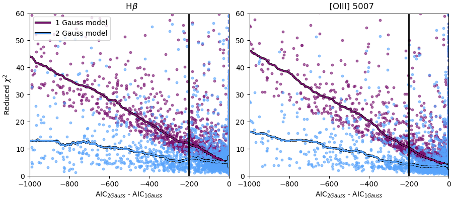
Figure 8: The reduced $\chi^{2}$ value plotted against the difference in BIC for fits to H$\beta$ (left) and [OIII] 5007 (right) emission lines. Purple points represent fits using a simple 1 Gaussian model. Blue points represent fits to the same data using a 2 Gaussian model. Solid lines of the same colour show the rolling median of the points. The vertical black line is the threshold value used for the whole sample, $\delta_{\rm BIC}=-200$. At this threshold, the two populations of fits are statistically different.

To find the optimum threshold value to use with our data, we first ran threadcount with a lenient threshold of $\delta_{\rm BIC}=-10$ for all galaxies in our sample. We then compared the reduced $\chi^{2}$ ($\chi^{2}_{red}=\chi^{2}/\nu$, where $\nu$ is the degrees of freedom) value from fits to the emission lines using both a simple 1 Gaussian model and a 2 Gaussian model to the $\delta_{\rm BIC}$ returned comparing the two models. There is some degree of circularity in this reasoning for any individual emission line fit, as the $\chi^{2}$ value is calculated as part of the BIC. However, we are using the comparative difference in $\chi^{2}_{red}$ value in order to understand the BIC values. 8 shows the $\chi^{2}_{red}$ value plotted against the $\delta_{\rm BIC}$ for all galaxies, with fits to H$\beta$ represented in the left, and [OIII] $\lambda 5007$ in the right panels respectively.

For each galaxy, we determined the threshold to be the maximum $\delta_{\rm BIC}$ where the running median of the $\chi^{2}_{red}$ for the 1 Gaussian models becomes one standard deviation away from the running median of the $\chi^{2}_{red}$ for the 2 Gaussian models. We then took the average across all galaxies, finding an average H$\beta$ threshold of -161, and an average [OIII] $\lambda 5007$ threshold of -132. We make a conservative choice to round to $\delta_{\rm BIC}=-200$ for our threshold value across the sample, and this is plotted as a black vertical line in Fig. 8. This conservative choice may bias results by removing fits to low signal-to-noise spectra, as well as fits suggesting low-velocity winds.

Appendix B Individual Galaxy Correlations

Galaxy Name	$v_{\rm out,[OIII]}$		$v_{\rm out,H\beta}$		$\dot{M}_{\rm out}$			$\dot{\Sigma}_{\rm out}$		$\eta$
	(km s-1)		(km s-1)		($M_{\odot}$ yr-1)			($M_{\odot}$ yr-1 kpc-2)
	Median	RMS	Median	RMS	Total	Median	RMS	Median	RMS	Total	Median	RMS
IRAS 08339+6517	264	268	223	236	26.3	0.04	0.25	0.75	4.27	2.82	3.23	4.31
IRAS 15229+0511	–	–	218	219	0.74	0.05	0.07	0.12	0.19	0.16	0.42	0.60
KISSR 1084	353	355	299	286	0.64	0.01	0.06	0.04	0.18	0.19	0.47	1.21
NGC 7316	136	136	118	169	0.45	0.01	0.02	0.06	0.14	0.15	1.03	1.67
UGC 01385	377	361	307	320	12.23	0.18	0.55	1.68	5.04	1.72	2.81	4.58
UGC 10099	233	283	190	210	3.37	0.03	0.08	0.08	0.22	0.70	1.05	1.46
CGCG 453-062	299	299	231	265	0.81	0.03	0.04	0.14	0.20	0.04	0.48	1.28
UGC 12150	–	–	138	138	0.01	0.01	0.01	0.04	0.04	0.0003	0.06	0.06
IRAS 20351+2521	146	269	211	248	0.57	0.03	0.06	0.08	0.16	0.03	0.22	0.40
NGC 0695	215	219	190	199	2.89	0.04	0.07	0.12	0.20	0.07	0.61	1.16

Table 4: The median and root-mean-square for the maximum outflow velocity $v_{\rm out}$ measured from the [OIII] $\lambda 5007$ and H$\beta$ emission lines; the total, median and root-mean-square mass outflow rate $\dot{M}_{\rm out}$; the median and root-mean-square mass outflow flux $\dot{\Sigma}_{\rm out}$; and the total, median and root-mean-square mass loading factor $\eta$ within $r_{90}$ for 10 face-on galaxies in the DUVET sample.

In this appendix, we show the correlations between the SFR surface density and the maximum outflow velocity from fits to the H$\beta$ and [OIII] $\lambda 5007$ emission lines, and the mass outflow flux for each individual galaxy in our sample. In each figure, the panels are organised from left to right and then top to bottom, such that the lowest total galaxy mass is in the top left panel and the highest total galaxy mass in the bottom right panel. Total galaxy masses for the galaxies are taken from literature values, and are given in Table 1. The median and root-mean-square scatter values for the outflow velocities and mass outflow flux, and the total, median and root-mean-square scatter values for the mass outflow rate and mass loading factor within $r_{90}$ for each galaxy are given in Table 4.

In Fig. 9 and Fig. 10 we compare the maximum outflow velocity to the SFR surface density for H$\beta$ and [OIII] $\lambda 5007$ respectively for each galaxy in our sample. All of the galaxies in our sample except for IRAS 08339+6517 are brighter in H$\beta$ than in [OIII] $\lambda 5007$. Three of our galaxies (UGC 12150, NGC 7316 and IRAS 15229+0511) do not have the signal-to-noise necessary to fit an outflow component in [OIII] $\lambda 5007$. In fact, we find only one spaxel in UGC 12150 where H$\beta$ is fit with an outflow component.

CGCG 453-062’s high inclination angle ($i\approx 54^{\circ}$) required that the velocities be deprojected by dividing by $\cos{i}$. The originally observed velocities are shown in the CGCG 453-062 panels of Fig. 9 and Fig. 10 as transparent orange circles. The deprojected velocities are shown as blue points. The median H$\beta$ outflow velocity before correction is 125 km s^-1, and the inclination correction increases this to 213 km s^-1.

In Fig. 4 we compare the ionised gas mass outflow flux to the SFR surface density for each galaxy in our sample. We show here the results for the outflow flux with no extinction correction applied (see Section 4.2 for more information on the extinction correction). We find that the majority of galaxies in our sample follow a trend of increasing outflow mass flux with increasing SFR surface density. This suggests that the important global change between galaxies is the degree of star formation driving the outflows, but on smaller scales the same local relationship remains.

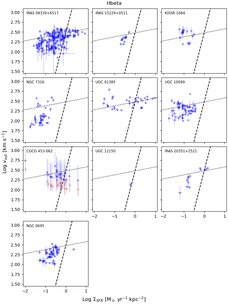
Figure 9: The maximum outflow velocity, $v_{\rm out}$, calculated using the H$\beta$ line plotted against the star formation rate surface density, $\Sigma_{\rm SFR}$ for individual galaxies in our sample, given in order of increasing total stellar mass from left to right, top to bottom. Orange points show the velocities we observe before reprojection. The dashed lines represent a model where outflows are primarily driven by momentum injected into the gas from young massive stars ($v_{\rm out}\propto\Sigma_{\rm SFR}^{2}$; Murray et al., 2011). The dotted lines represent a model where outflows are primarily driven by energy injected from supernovae ($v_{\rm out}\propto\Sigma_{\rm SFR}^{0.1}$; Chen et al., 2010).

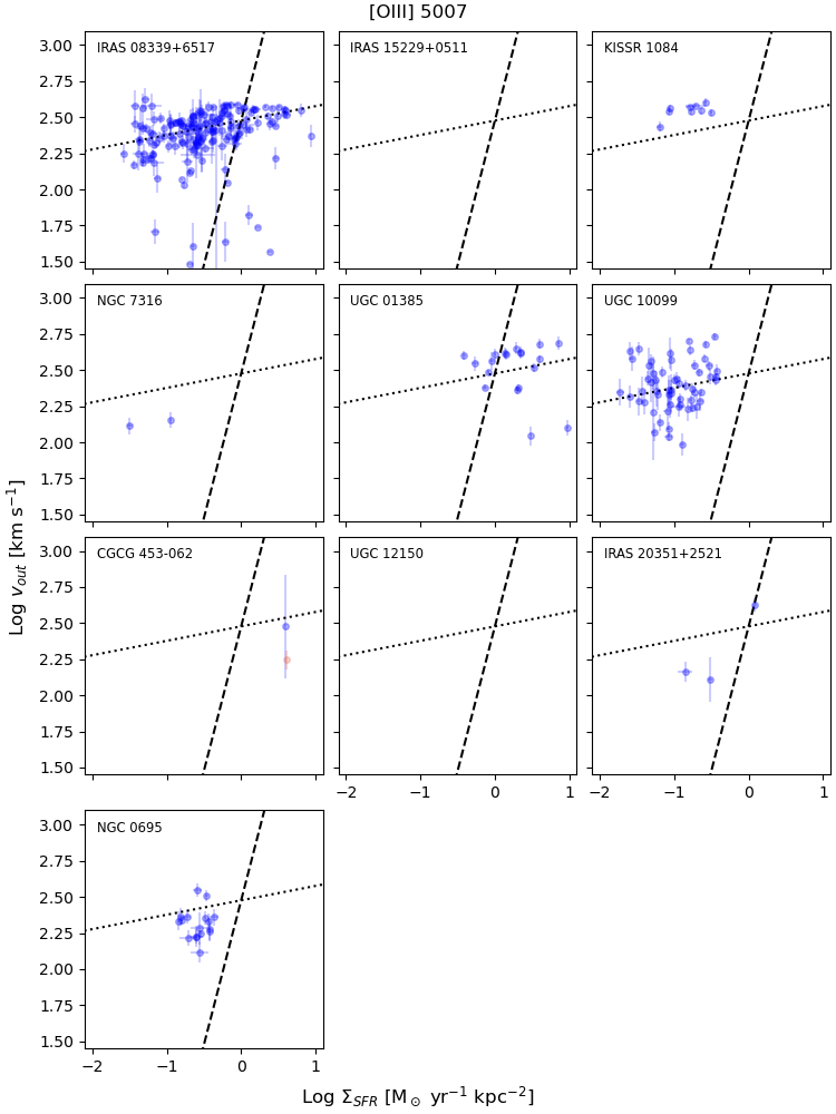
Figure 10: As for Fig. 9, but using results from fits to the [OIII] $\lambda 5007$ emission line.

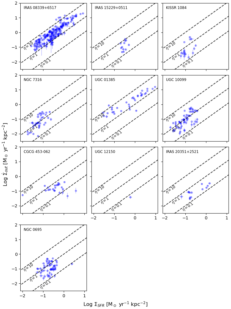
Figure 11: The ionised gas outflow mass flux, $\dot{\Sigma}_{\rm out}$, compared to the SFR surface density, $\Sigma_{\rm SFR}$, for spaxels of sub-kpc resolution pixels in local starbursting disk galaxies with evidence for outflow components. Each panel gives results for a different galaxy in our sample, given in order of increasing total stellar mass from left to right, top to bottom. Dashed black lines show constant mass loading factors.

References

- Anglés-Alcázar et al. (2017) Anglés-Alcázar D., Faucher-Giguère C.-A., Kereš D., Hopkins P. F., Quataert E., Murray N., 2017, MNRAS, 470, 4698
- Arribas et al. (2014) Arribas S., Colina L., Bellocchi E., Maiolino R., Villar-Martín M., 2014, A&A, 568, A14
- Avery et al. (2021) Avery C. R., et al., 2021, MNRAS,
- Avery et al. (2022) Avery C. R., et al., 2022, MNRAS, 511, 4223
- Bik et al. (2022) Bik A., Östlin G., Hayes M., Melinder J., Menacho V., 2022, A&A, 666, A161
- Bolatto et al. (2013) Bolatto A. D., et al., 2013, Nature, 499, 450
- Bordoloi et al. (2014) Bordoloi R., et al., 2014, ApJ, 794, 130
- Calzetti (2001) Calzetti D., 2001, PASP, 113, 1449
- Cameron et al. (2021) Cameron A. J., et al., 2021, ApJ, 918, L16
- Cappellari (2017) Cappellari M., 2017, MNRAS, 466, 798
- Cardelli et al. (1989) Cardelli J. A., Clayton G. C., Mathis J. S., 1989, ApJ, 345, 245
- Chen et al. (2010) Chen Y.-M., Tremonti C. A., Heckman T. M., Kauffmann G., Weiner B. J., Brinchmann J., Wang J., 2010, AJ, 140, 445
- Chevance et al. (2022) Chevance M., et al., 2022, MNRAS, 509, 272
- Chisholm et al. (2015) Chisholm J., Tremonti C. A., Leitherer C., Chen Y., Wofford A., Lundgren B., 2015, ApJ, 811, 149
- Chisholm et al. (2017) Chisholm J., Tremonti C. A., Leitherer C., Chen Y., 2017, Monthly Notices of the Royal Astronomical Society, 469, 4831
- Cluver et al. (2017) Cluver M. E., Jarrett T. H., Dale D. A., Smith J. D. T., August T., Brown M. J. I., 2017, ApJ, 850, 68
- Concas et al. (2022) Concas A., et al., 2022, MNRAS, 513, 2535
- Conroy (2013) Conroy C., 2013, ARA&A, 51, 393
- Cook et al. (2019) Cook D. O., et al., 2019, ApJ, 880, 7
- Crocker et al. (2021) Crocker R. M., Krumholz M. R., Thompson T. A., 2021, MNRAS, 503, 2651
- Cutri et al. (2021) Cutri R. M., et al., 2021, VizieR Online Data Catalog, p. II/328
- Davies et al. (2019) Davies R. L., et al., 2019, ApJ, 873, 122
- Davies et al. (2021) Davies R. L., et al., 2021, ApJ, 909, 78
- Engelbracht et al. (2006) Engelbracht C. W., et al., 2006, ApJ, 642, L127
- Eskew et al. (2012) Eskew M., Zaritsky D., Meidt S., 2012, AJ, 143, 139
- Faucher-Giguère et al. (2013) Faucher-Giguère C.-A., Quataert E., Hopkins P. F., 2013, MNRAS, 433, 1970
- Fernández Lorenzo et al. (2013) Fernández Lorenzo M., Sulentic J., Verdes-Montenegro L., Argudo-Fernández M., 2013, MNRAS, 434, 325
- Fielding et al. (2017) Fielding D., Quataert E., Martizzi D., Faucher-Giguère C.-A., 2017, MNRAS, 470, L39
- Fielding et al. (2018) Fielding D., Quataert E., Martizzi D., 2018, MNRAS, 481, 3325
- Fisher et al. (2019) Fisher D. B., Bolatto A. D., White H., Glazebrook K., Abraham R. G., Obreschkow D., 2019, ApJ, 870, 46
- Fisher et al. (2022) Fisher D. B., Bolatto A. D., Glazebrook K., Obreschkow D., Abraham R. G., Kacprzak G. G., Nielsen N. M., 2022, ApJ, 928, 169
- Fluetsch et al. (2019) Fluetsch A., et al., 2019, MNRAS, 483, 4586
- Fluetsch et al. (2021) Fluetsch A., et al., 2021, MNRAS, 505, 5753
- Förster Schreiber et al. (2019) Förster Schreiber N. M., et al., 2019, ApJ, 875, 21
- Galván-Madrid et al. (2012) Galván-Madrid R., Goddi C., Rodríguez L. F., 2012, A&A, 547, L3
- Girard et al. (2021) Girard M., et al., 2021, ApJ, 909, 12
- Girichidis et al. (2016) Girichidis P., et al., 2016, ApJ, 816, L19
- Girichidis et al. (2024) Girichidis P., Werhahn M., Pfrommer C., Pakmor R., Springel V., 2024, MNRAS, 527, 10897
- Greco et al. (2012) Greco J. P., Martini P., Thompson T. A., 2012, ApJ, 757, 24
- Hao et al. (2011) Hao C.-N., Kennicutt R. C., Johnson B. D., Calzetti D., Dale D. A., Moustakas J., 2011, ApJ, 741, 124
- Hayward & Hopkins (2017) Hayward C. C., Hopkins P. F., 2017, MNRAS, 465, 1682
- Heckman et al. (2000) Heckman T. M., Lehnert M. D., Strickland D. K., Armus L., 2000, ApJS, 129, 493
- Heckman et al. (2002) Heckman T., Mulchaey J., Stocke J., 2002, in ASP Conference Proceedings. p. 292
- Hinshaw et al. (2013) Hinshaw G., et al., 2013, ApJS, 208, 19
- Ho et al. (2014) Ho I. T., et al., 2014, MNRAS, 444, 3894
- Hopkins et al. (2012) Hopkins P. F., Quataert E., Murray N., 2012, MNRAS, 421, 3522
- Hopkins et al. (2014) Hopkins P. F., Kereš D., Oñorbe J., Faucher-Giguère C.-A., Quataert E., Murray N., Bullock J. S., 2014, MNRAS, 445, 581
- Howell et al. (2010) Howell J. H., et al., 2010, ApJ, 715, 572
- Kaasinen et al. (2017) Kaasinen M., Bian F., Groves B., Kewley L. J., Gupta A., 2017, MNRAS, 465, 3220
- Kass & Raftery (1995) Kass R. E., Raftery A. E., 1995, Journal of the American Statistical Association, 90, 773
- Keto et al. (2008) Keto E., Zhang Q., Kurtz S., 2008, ApJ, 672, 423
- Kim & Ostriker (2017) Kim C.-G., Ostriker E. C., 2017, ApJ, 846, 133
- Kim & Ostriker (2018) Kim C.-G., Ostriker E. C., 2018, ApJ, 853, 173
- Kim et al. (2020) Kim C.-G., et al., 2020, ApJ, 900, 61
- Kim et al. (2023) Kim C.-G., Kim J.-G., Gong M., Ostriker E. C., 2023, ApJ, 946, 3
- Kornei et al. (2012) Kornei K. A., Shapley A. E., Martin C. L., Coil A. L., Lotz J. M., Schiminovich D., Bundy K., Noeske K. G., 2012, ApJ, 758, 135
- Kouroumpatzakis et al. (2021) Kouroumpatzakis K., Zezas A., Maragkoudakis A., Willner S. P., Bonfini P., Ashby M. L. N., Sell P. H., Jarrett T. H., 2021, MNRAS, 506, 3079
- Kroupa & Weidner (2003) Kroupa P., Weidner C., 2003, ApJ, 598, 1076
- Krumholz et al. (2018) Krumholz M. R., Burkhart B., Forbes J. C., Crocker R. M., 2018, MNRAS, 477, 2716
- Li et al. (2017) Li M., Bryan G. L., Ostriker J. P., 2017, ApJ, 841, 101
- López-Sánchez et al. (2006) López-Sánchez Á. R., Esteban C., García-Rojas J., 2006, A&A, 449, 997
- Marasco et al. (2023) Marasco A., et al., 2023, A&A, 670, A92
- Martin (2005) Martin C. L., 2005, ApJ, 621, 227
- McLeod et al. (2021) McLeod A. F., et al., 2021, MNRAS, 508, 5425
- McPherson et al. (2023) McPherson D. K., et al., 2023, MNRAS, 525, 6170
- McQuinn et al. (2019) McQuinn K. B. W., van Zee L., Skillman E. D., 2019, ApJ, 886, 74
- Meidt et al. (2012) Meidt S. E., et al., 2012, ApJ, 744, 17
- Morrissey et al. (2018) Morrissey P., et al., 2018, ApJ, 864, 93
- Murray et al. (2005) Murray N., Quataert E., Thompson T. A., 2005, ApJ, 618, 569
- Murray et al. (2011) Murray N., Ménard B., Thompson T. A., 2011, ApJ, 735, 66
- Naab & Ostriker (2017) Naab T., Ostriker J. P., 2017, ARA&A, 55, 59
- Nelson et al. (2019) Nelson D., et al., 2019, MNRAS, 490, 3234
- Newman et al. (2012) Newman S. F., et al., 2012, ApJ, 761, 43
- Newville et al. (2019) Newville M., et al., 2019, lmfit/lmfit-py 0.9.14, doi:10.5281/zenodo.3381550
- Oppenheimer & Davé (2006) Oppenheimer B. D., Davé R., 2006, MNRAS, 373, 1265
- Orr et al. (2022) Orr M. E., Fielding D. B., Hayward C. C., Burkhart B., 2022, ApJ, 924, L28
- Osterbrock & Ferland (2006) Osterbrock D. E., Ferland G. J., 2006, Astrophysics of gaseous nebulae and active galactic nuclei. University Science Books
- Ostriker & Kim (2022) Ostriker E. C., Kim C.-G., 2022, ApJ, 936, 137
- Ostriker et al. (2010) Ostriker E. C., McKee C. F., Leroy A. K., 2010, ApJ, 721, 975
- Pandya et al. (2021) Pandya V., et al., 2021, MNRAS, 508, 2979
- Prusinski et al. (2021) Prusinski N. Z., Erb D. K., Martin C. L., 2021, AJ, 161, 212
- Rathjen et al. (2023) Rathjen T.-E., Naab T., Walch S., Seifried D., Girichidis P., Wünsch R., 2023, MNRAS, 522, 1843
- Reichardt Chu et al. (2022a) Reichardt Chu B., et al., 2022a, MNRAS, 511, 5782
- Reichardt Chu et al. (2022b) Reichardt Chu B., et al., 2022b, ApJ, 941, 163
- Roberts-Borsani et al. (2020) Roberts-Borsani G. W., Saintonge A., Masters K. L., Stark D. V., 2020, MNRAS, 493, 3081
- Roussel et al. (2010) Roussel H., et al., 2010, A&A, 518, L66
- Rozas et al. (2007) Rozas M., Richer M. G., Steffen W., García-Segura G., López J. A., 2007, A&A, 467, 603
- Rubin et al. (2010) Rubin K. H. R., Weiner B. J., Koo D. C., Martin C. L., Prochaska J. X., Coil A. L., Newman J. A., 2010, ApJ, 719, 1503
- Rubin et al. (2014) Rubin K. H. R., Prochaska J. X., Koo D. C., Phillips A. C., Martin C. L., Winstrom L. O., 2014, ApJ, 794, 156
- Rupke et al. (2005) Rupke D. S., Veilleux S., Sanders D. B., 2005, ApJS, 160, 115
- Salpeter (1955) Salpeter E. E., 1955, ApJ, 121, 161
- Sánchez et al. (2021) Sánchez S. F., et al., 2021, MNRAS, 503, 1615
- Schlafly & Finkbeiner (2011) Schlafly E. F., Finkbeiner D. P., 2011, ApJ, 737, 103
- Schneider et al. (2018) Schneider E. E., Robertson B. E., Thompson T. A., 2018, ApJ, 862, 56
- Shangguan et al. (2019) Shangguan J., Ho L. C., Li R., Zhuang M.-Y., Xie Y., Li Z., 2019, ApJ, 870, 104
- Somerville & Davé (2015) Somerville R. S., Davé R., 2015, ARA&A, 53, 51
- Springel & Hernquist (2003) Springel V., Hernquist L., 2003, MNRAS, 339, 289
- Stanway & Eldridge (2018) Stanway E. R., Eldridge J. J., 2018, MNRAS, 479, 75
- Steidel et al. (2010) Steidel C. C., Erb D. K., Shapley A. E., Pettini M., Reddy N., Bogosavljević M., Rudie G. C., Rakic O., 2010, ApJ, 717, 289
- Sun et al. (2023) Sun J., et al., 2023, ApJ, 945, L19
- Swinbank et al. (2019) Swinbank A. M., et al., 2019, MNRAS, 487, 381
- Tumlinson et al. (2017) Tumlinson J., Peeples M. S., Werk J. K., 2017, ARA&A, 55, 389
- Veilleux et al. (2005) Veilleux S., Cecil G., Bland-Hawthorn J., 2005, ARA&A, 43, 769
- Veilleux et al. (2020) Veilleux S., Maiolino R., Bolatto A. D., Aalto S., 2020, A&ARv, 28, 2
- Vijayan et al. (2020) Vijayan A., Kim C.-G., Armillotta L., Ostriker E. C., Li M., 2020, ApJ, 894, 12
- Walcher et al. (2009) Walcher C. J., Coelho P., Gallazzi A., Charlot S., 2009, MNRAS, 398, L44
- Wright et al. (2010) Wright E. L., et al., 2010, AJ, 140, 1868
- Xu et al. (2022) Xu X., et al., 2022, ApJ, 933, 222
- Xu et al. (2023) Xu X., Heckman T., Yoshida M., Henry A., Ohyama Y., 2023, ApJ, 956, 142
- van de Sande et al. (2023) van de Sande J., Fraser-McKelvie A., Fisher D. B., Martig M., Hayden M. R., the GECKOS Survey collaboration 2023, arXiv e-prints, p. arXiv:2306.00059