Testing the isotropy of cosmic acceleration with Pantheon+SH0ES: A cosmographic analysis
Abstract
We use a recent Pantheon+SH0ES compilation of Type Ia Supernova distance measurements at low-redshift, i.e., , in order to investigate the directional dependency of the deceleration parameter () in different patches ( size) across the sky, as a probe of the statistical isotropy of the Universe. We adopt a cosmographic approach to compute the cosmological distances, fixing and to reference values provided by the collaboration. By looking at 500 different patches randomly taken across the sky, we find a maximum CL anisotropy level for , whose direction points orthogonally to the CMB dipole axis, i.e., vs . We assessed the statistical significance of those results, finding that such a signal is expected due to the limitations of the observational sample. These results support that there is no significant evidence for a departure from the cosmic isotropy assumption, one of the pillars of the standard cosmological model.
pacs:
98.65.Dx, 98.80.EsI Introduction
One of the foundations of the current standard cosmological model, also known as - Cold Dark Matter (CDM) scenario, is the assumption of the validity of the Cosmological Principle (CP) at large scales Goodman:1995dt ; Clarkson:2010uz ; Maartens:2011yx ; Clarkson:2012bg ; Aluri:2022hzs . In other words, it states that the Universe should appear statistically homogeneous and isotropic at those scales, so that we can measure cosmological distances and ages using the Friedmann-Lemaître-Robertson-Walker (FLRW) metric. Recent analysis of redshift surveys of galaxies and quasars indicate that there is indeed a transition scale from a locally inhomogeneous Universe to a smoother, statistically homogeneous one, as described by the CP, at about 70-120 Mpc Laurent:2016eqo ; Ntelis:2017nrj ; Goncalves:2017dzs ; Goncalves:2020erb ; Kim:2021osl ; Andrade:2022imy .
Hence, we must test the assumption of the cosmological isotropy as well in order to confirm (or rule out) the CP as a valid physical assumption. If ruled out, the standard model would require a profound reformulation of its basic hypotheses, including the physical origin of the mechanism behind cosmic acceleration. One possible way to test such a hypothesis involves analyzing the cosmological parameters’ directional dependency, as estimated from the luminosity distance measurements of Type Ia Supernova (SNe). This method has been explored since the release of the earliest SN compilations, using a variety of approaches, yielding inconclusive results due to the limited sampling of objects – in terms of small number of SNe available, distance measurement uncertainties, and especially uneven sky coverage Kolatt:2000yg ; Schwarz:2007wf ; Antoniou:2010gw ; Cai:2011xs ; Bahr-Kalus:2012yjc ; Zhao:2013yaa ; BeltranJimenez:2014otq ; Chang:2014wpa ; Bengaly:2015dza ; Javanmardi:2015sfa ; Deng:2018jrp ; Andrade:2018eta ; Colin:2019opb ; Zhao:2019azy ; Kazantzidis:2020tko ; Hu:2020mzd ; Salehi:2020hek ; Zhao:2021fcp ; Krishnan:2021jmh ; Horstmann:2021jjg ; Rahman:2021mti ; Dhawan:2022lze . The latest SN compilation, namely the Pantheon+SH0ES data-set Brout:2022vxf (see also Scolnic:2021amr ; Riess:2021jrx ), provides 1701 light curve measurements of 1550 SN objects. This corresponds to a significant improvement from previous figures of earlier SN compilations – for instance, the previous Pantheon and JLA compilations comprised 1048 and 740 SN distance measurements, respectively. However, recent analyses still yield inconclusive results regarding the validity of cosmic isotropy, depending on the sample selection and the methodology adopted Sorrenti:2022zat ; Cowell:2022ehf ; Pasten:2023rpc ; McConville:2023xav ; Perivolaropoulos:2023tdt ; Tang:2023kzs ; Hu:2023eyf .
Given this scenario, we look further at the isotropy of the Pantheon+SH0ES data. In this case, we carry out a directional analysis of the deceleration parameter () across the celestial sphere. Similar approaches were adopted in McConville:2023xav ; Hu:2023eyf , although the authors focused on the and parameters, as given by the standard model, i.e., within the flat CDM framework. Instead, we rely on a cosmographic description of the Universe so that no further assumptions on its dynamic content, e.g., the nature of dark matter and dark energy, are needed – as long as we restrict our analysis to the lower redshift threshold of the sample. We also estimate the statistical significance of our results in light of the assumptions made on data analysis, or the non-uniformity of the SN sky distribution.
The paper is structured as follows: Section II is dedicated to explaining our method and the data selection and preparation. Section III presents the results obtained from this method, along with the statistical significance tests. Section IV provides the discussion and our concluding remarks.
II Method
II.1 Data Preparation
We use the Pantheon+SH0ES compilation, as retrieved from the Github repository111https://github.com/PantheonPlusSH0ES/DataRelease. This data set consists on 1701 light curve measurements of 1550 distinct SNe within the redshift range, which also comprises 77 data points from Cepheid host galaxies at very low redshifts, i.e., . Those measurements are designated in the data release as a boolean variable, so that we use the Cepheid host distances provided in those cases, instead of the distance modulus measured by the corresponding SN. Note we use the redshift given in the zHD variable, since it includes the correction from the heliocentric to the Cosmic Microwave Background rest-frame, as well as further corrections due to the nearby SN peculiar velocities Peterson:2021hel ; Carr:2021lcj . Still, we caution that the effect of those peculiar velocities can lead to spurious anisotropy in the Hubble Flow, if not properly accounted for Hellwing:2016pdl ; Bengaly:2018uqp ; Kalbouneh:2022tfw ; Maartens:2023tib ; Kalbouneh:2024szq . Although some doubts have been cast on the modelling of the SN peculiar velocities in this sample (see Sorrenti:2022zat ), we will not attempt to reevaluate their effects on the isotropy test we perform in this work.
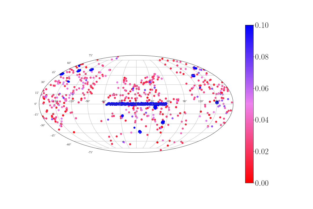
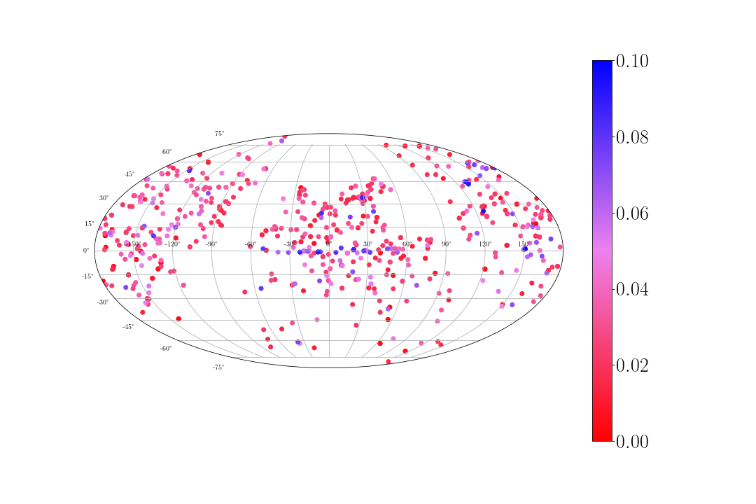
It is important to avoid possible biases from the original sample as much as possible, because it consists of an SN compilation from observations performed by various surveys that have (or had) different designs and sky coverage. Thus, the original SN compilation is expected to be affected mainly by uneven sky coverage. Due to this, we impose two different redshift cutoffs before we proceed to the isotropy test. The first one consists of an upper redshift cutoff at the range, since the SN sky distribution becomes much more sparse at higher redshifts (see upper panel of Fig. 1 for a visual explanation). This is something expected, since those objects were observed by spectroscopic surveys designed to cover only those specific regions of the sky, in order to obtain the highest-resolution spectroscopy possible. Also, we can safely use cosmographic expansion on equation 1 since it is a good approximation in that redshift range. Secondly, we impose a lower redshift cutoff at , except for the distance measurements within Cepheid host galaxies. Hence, we end up with a working sample of 697 SN data points, as displayed in the lower panel of Fig. 1.
II.2 Estimator
We assume a cosmographic expression of the luminosity distance Weinberg:1972kfs ; Visser:2003vq ; Cattoen:2007id
| (1) |
where and stand for the Hubble Constant and the deceleration parameter, respectively, and is given in Mpc. As the distance modulus definition reads
| (2) |
we obtain the best-fit for the through a minimization, as given by
| (3) |
so that denotes the full SN covariance matrix, and
| (4) |
We adopt the following estimator to test the isotropy of the local cosmic acceleration by a similar fashion of McConville:2023xav ; Hu:2023eyf , as follows
| (5) |
where is given in units of confidence level (CL). We compute the best-fitted value for the deceleration parameters at opposite patches across the entire celestial sphere ( size) along a specific axis randomly selected across the sky. A total of 500 axes were taken in our analysis. In Eq. 5, these quantities are denoted by , and , correspondingly, while and provides their respective uncertainties at CL. We stress that we perform our analysis within size spherical caps, instead of size ones – which encompasses an entire hemisphere – for the sake of computational time. Nonetheless, we expect that this choice should not impact our conclusions, as the results obtained from caps show good agreement with those assuming caps – see Fig. 18 in Hu:2023eyf
III Results
III.1 Real data analysis
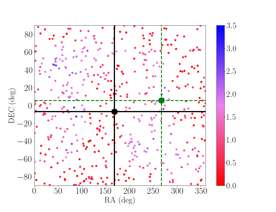
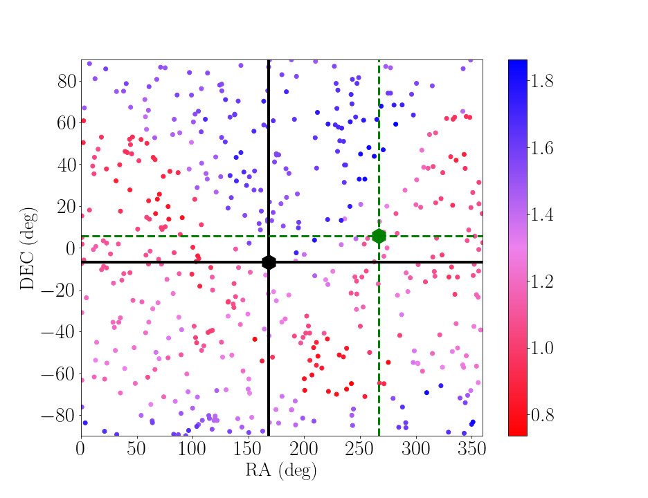
We show the result of the analysis in the left panel of Fig. 2. We represent it as a map in Cartesian coordinates of the values obtained across the 500 randomly selected directions in the sky for the Pantheon+SH0ES SN sample. Here, is given in units of standard deviations. The green diamond mark displays the maximum anisotropy direction found, along the axis, as represented by the green dashed lines, while the black solid lines and black dotted mark represents the CMB dipole direction, i.e., . We report a maximum value of in this case.
For the sake of consistency, we also display the reduced value in the right panel of the same figure, as defined by , where denotes the number of degrees of freedom in each celestial cap, and is given by Eq. 3. We can see that the bluest dots, which denote the poorest fits to the data, does not coincide with the bluest regions in the map. This result indicates that the larger values do not occur due to a poor fit of the data.
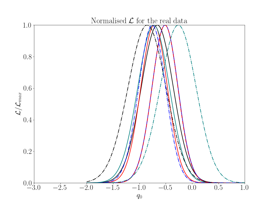
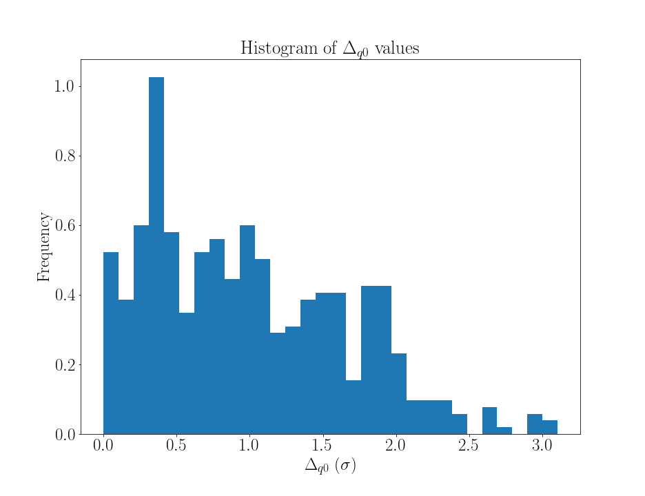
Accordingly, in the left panel of Fig. 3, we present examples of the normalised likelihood functions obtained from four different directions in the sky to visualize better the fits. In this case, different colours denote different sky directions, whereas the solid and dashed-dotted curves stand for the “northern” and “southern” counterpart of each direction respectively. In addition, the right panel of the same figure shows a histogram of the values, as given in confidence levels. We find that this distribution peaks at , which corresponds to the most frequent value for the anisotropy level, and that its maximum value is – as also shown in the left panel of Fig. 2.
III.2 Statistical significance of the results
As for the statistical significance of our results, we test three main cases: (i) How the values can be affected under the assumption of different values to be fixed in our analysis; (ii) How the values can be affected when assuming a fiducial value; (iii) How the values can be affected if the SN celestial distribution is considered uniform. In all three cases, we stress that we are assuming the same SN covariance matrix as the original one, apart from the redshift selection imposed.
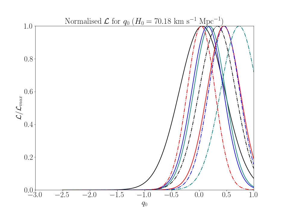
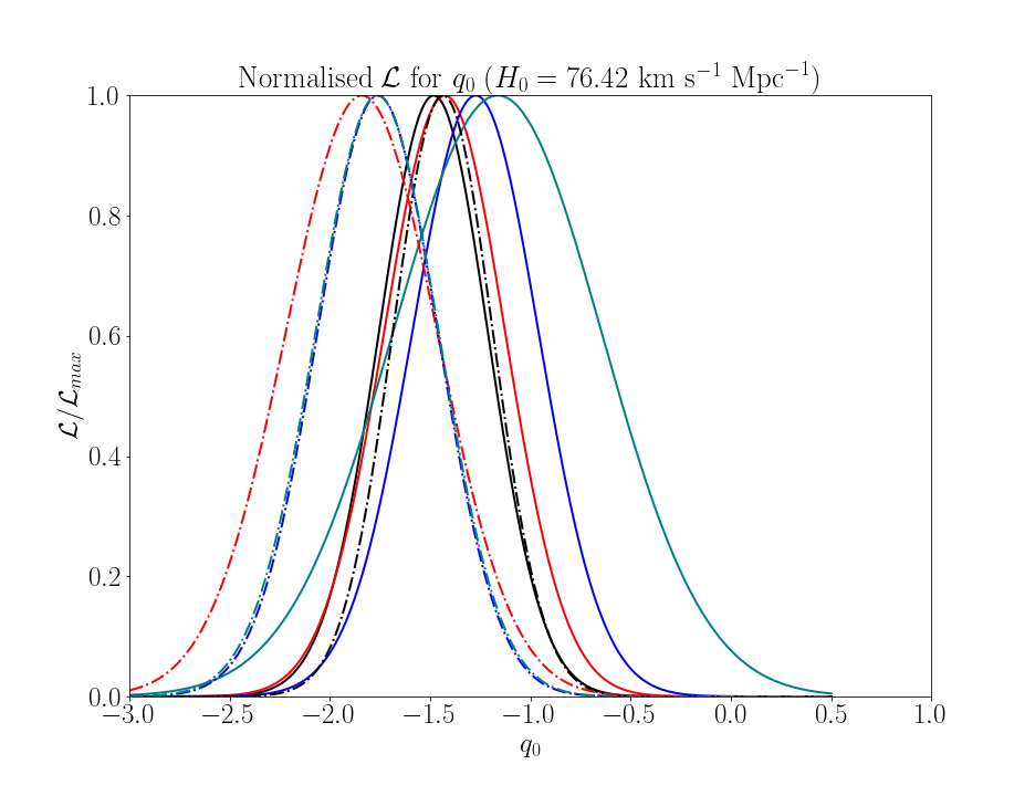
As for case (i): In Fig. 4, we display the normalised likelihoods for when assuming different Hubble Constant values, i.e., (left panel), and (right panel). We find that a higher value leads to highly negative values for the deceleration parameter. In contrast, the opposite trend occurs for lower values – see how those likelihoods are skewed to the right and left, respectively, compared to those shown in the left panel of Fig. 3, where we assumed the SH0ES measurement. Hence, we find that the fit is very sensitive to the assumption, which is an expected result, since this parameter is degenerated with the absolute magnitude value – and so we would need to adjust accordingly to the change in the . We will leave a more thorough examination of the possible degeneracy in the plane in a future work.
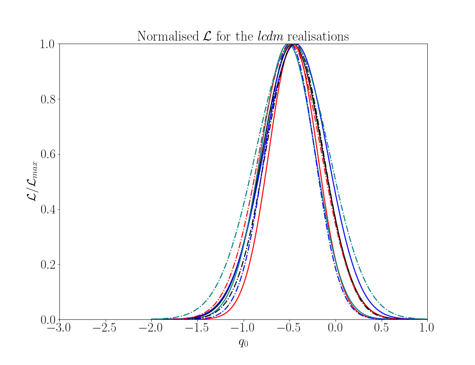
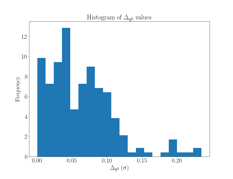
As for case (ii): In Fig. 5, we show the results obtained by means of a set of 200 realisations named lcdm. In this case, we fixed the observed modulus distance to the value given by the flat CDM best-fit for from the original Pantheon+SH0ES, i.e., , as and thus . The goal is to assess the residuals of our best-fit estimator due to the limited sampling of SNe across the sky given our patch size. As we can see in its left panel, we are able to robustly recover the fiducial best-fit in all cases, albeit with larger uncertainty in some of them – which naturally occur due to the SN sky sampling in those specific patches. On the other hand, the histogram displayed in the right panel shows a maximum value of in those realisations. We interpret this result as the maximum variance we can expect from our analysis due only to the effect of the SN sample incompleteness across the celestial sphere.
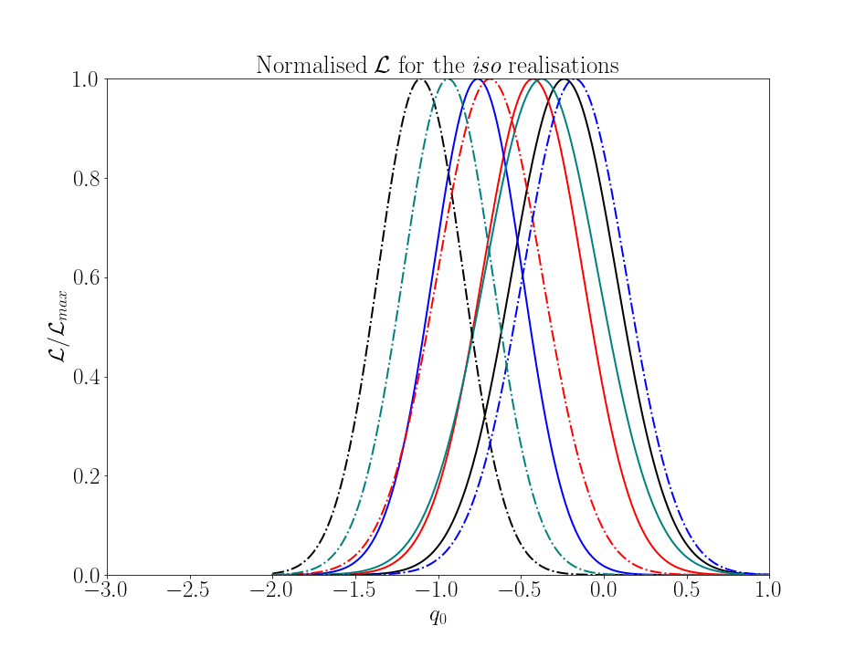
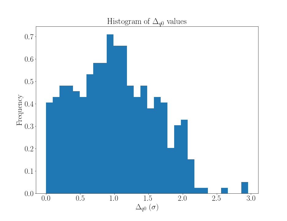
As for case (iii): In Fig. 6, we present normalised for 5 realisations (left panel), and the histogram (right panel) for a set of 400 iso realisations. Conversely, from the previous cases, we assume a uniform SN sky distribution by replacing the original SN coordinates with a random direction across the celestial sphere. We obtain a maximum value of in this case. Such a result is in good agreement with the result obtained for the real data case – especially considering the residual obtained for the lcdm realisations, as previously described. Therefore, we conclude that there is no statistically significant indication for a breakdown of the cosmic isotropy hypothesis in this case.
IV Discussion and conclusions
The validity of the Cosmological Principle, i.e., the large-scale isotropy and homogeneity of the Universe, constitutes one of the core assumptions of modern Cosmology. Even though the available observational data favours the CDM scenario based on this hypothesis, it has seldom been tested directly. Hence, developing and performing such tests is crucial since any hint of a statistically significant breakdown of such an assumption would require an extensive reformulation of the standard cosmological model from the basics.
We used the latest Type Ia Supernova compilation of distance measurements, namely the Pantheon+SH0ES data set to test the isotropy of the Universe. We did so by assessing the directional dependence of the deceleration parameter, where we split the data into sub-sets across randomly selected directions in the sky, in which we obtained their best-fitted values. After restricting our data to the range, except for the SN in Cepheid host galaxies, we found a maximum variation of at roughly from the CMB dipole direction – a signal ascribed to our relative motion concerning its rest frame. Moreover, we found that this result does not manifest from the assumptions made during the parameter estimation – e.g., by fixing the Hubble Constant and SN absolute magnitude to its default values or by the incoherent fitting of the deceleration parameter – and most importantly, we found that such a variation is in good agreement with simulations assuming a uniform sky distribution of the SN data points. Therefore, we can conclude that this result is not statistically significant and that it should occur due to intrinsic fluctuations in the data – primarily due to the uncertainties in its covariance matrix.
Our results present an improvement from analyses made on the previous SN compilation, i.e., the Pantheon data set, where it was found from similar tests that the directional dependence of the cosmological parameters could be ascribed to the inhomogeneous SN celestial distribution - see, for instance, Andrade:2018eta . In addition, we extend and complement former analyses in the literature Pasten:2023rpc ; McConville:2023xav ; Perivolaropoulos:2023tdt ; Tang:2023kzs ; Hu:2023eyf , as we avoided the assumption of dark energy using the cosmographic expansion, and performed more stringent cuts in the sample to avoid possible biases. Hence, in contrast with some of those results, we found no significant evidence for a possible deviation from the Cosmological Principle assumption in the Pantheon+SH0ES data. This is in good agreement with previous tests using other types cosmological observations, e.g. galaxy clusters Bengaly:2015xkw , infrared galaxies Bengaly:2017zlo , Gamma Ray Bursts Andrade:2019kvl , and quasars Mittal:2023xub .
Given the advent of ongoing and forthcoming redshift surveys, such as eROSITA Merloni:2024zgn , Vera C. Rubin Observatory LSSTScience:2009jmu , Euclid Amendola:2016saw , Square Kilometer Array Observatory SKA:2018ckk , besides distance measurements by standard sirens from LIGO and Einstein Telescope, we expect that this variance should be reduced even further, and thus, we will be able to pinpoint if the Cosmological Principle provides a realistic representation of the Universe at large scales.
Acknowledgments: CB acknowledges financial support from Fundação à Pesquisa do Estado do Rio de Janeiro (FAPERJ) - Postdoc Recente Nota 10 (PDR10) fellowship. JSA is supported by CNPq grant No. 307683/2022-2 and Fundação de Amparo à Pesquisa do Estado do Rio de Janeiro (FAPERJ) grant No. 259610 (2021). This work was developed thanks to the National Observatory Data Center (CPDON).
References
- (1) J. Goodman, “Geocentrism reexamined,” Phys. Rev. D 52 (1995), 1821-1827 doi:10.1103/PhysRevD.52.1821 [arXiv:astro-ph/9506068 [astro-ph]].
- (2) C. Clarkson and R. Maartens, “Inhomogeneity and the foundations of concordance cosmology,” Class. Quant. Grav. 27 (2010), 124008 doi:10.1088/0264-9381/27/12/124008 [arXiv:1005.2165 [astro-ph.CO]].
- (3) R. Maartens, “Is the Universe homogeneous?,” Phil. Trans. Roy. Soc. Lond. A 369 (2011), 5115-5137 doi:10.1098/rsta.2011.0289 [arXiv:1104.1300 [astro-ph.CO]].
- (4) C. Clarkson, “Establishing homogeneity of the universe in the shadow of dark energy,” Comptes Rendus Physique 13 (2012), 682-718 doi:10.1016/j.crhy.2012.04.005 [arXiv:1204.5505 [astro-ph.CO]].
- (5) P. K. Aluri, P. Cea, P. Chingangbam, M. C. Chu, R. G. Clowes, D. Hutsemékers, J. P. Kochappan, A. M. Lopez, L. Liu and N. C. M. Martens, et al. “Is the observable Universe consistent with the cosmological principle?,” Class. Quant. Grav. 40 (2023) no.9, 094001 doi:10.1088/1361-6382/acbefc [arXiv:2207.05765 [astro-ph.CO]].
- (6) P. Laurent, J. M. Le Goff, E. Burtin, J. C. Hamilton, D. W. Hogg, A. Myers, P. Ntelis, I. Pâris, J. Rich and E. Aubourg, et al. “A 14 Gpc3 study of cosmic homogeneity using BOSS DR12 quasar sample,” JCAP 11 (2016), 060 doi:10.1088/1475-7516/2016/11/060 [arXiv:1602.09010 [astro-ph.CO]].
- (7) P. Ntelis, J. C. Hamilton, J. M. Le Goff, E. Burtin, P. Laurent, J. Rich, N. G. Busca, J. Tinker, E. Aubourg and H. Bourboux, et al. “Exploring cosmic homogeneity with the BOSS DR12 galaxy sample,” JCAP 06 (2017), 019 doi:10.1088/1475-7516/2017/06/019 [arXiv:1702.02159 [astro-ph.CO]].
- (8) R. S. Gonçalves, G. C. Carvalho, C. A. P. Bengaly, J. C. Carvalho, A. Bernui, J. S. Alcaniz and R. Maartens, “Cosmic homogeneity: a spectroscopic and model-independent measurement,” Mon. Not. Roy. Astron. Soc. 475 (2018) no.1, L20-L24 doi:10.1093/mnrasl/slx202 [arXiv:1710.02496 [astro-ph.CO]].
- (9) R. S. Gonçalves, G. C. Carvalho, U. Andrade, C. A. P. Bengaly, J. C. Carvalho and J. Alcaniz, “Measuring the cosmic homogeneity scale with SDSS-IV DR16 Quasars,” JCAP 03 (2021), 029 doi:10.1088/1475-7516/2021/03/029 [arXiv:2010.06635 [astro-ph.CO]].
- (10) Y. Kim, C. G. Park, H. Noh and J. c. Hwang, “CMASS galaxy sample and the ontological status of the cosmological principle,” Astron. Astrophys. 660 (2022), A139 doi:10.1051/0004-6361/202141909 [arXiv:2112.04134 [astro-ph.CO]].
- (11) U. Andrade, R. S. Gonçalves, G. C. Carvalho, C. A. P. Bengaly, J. C. Carvalho and J. Alcaniz, “The angular scale of homogeneity with SDSS-IV DR16 luminous red galaxies,” JCAP 10 (2022), 088 doi:10.1088/1475-7516/2022/10/088 [arXiv:2205.07819 [astro-ph.CO]].
- (12) T. S. Kolatt and O. Lahav, “Constraints on cosmological anisotropy out to z=1 from supernovae ia,” Mon. Not. Roy. Astron. Soc. 323 (2001), 859 doi:10.1046/j.1365-8711.2001.04262.x [arXiv:astro-ph/0008041 [astro-ph]].
- (13) D. J. Schwarz and B. Weinhorst, “(An)isotropy of the Hubble diagram: Comparing hemispheres,” Astron. Astrophys. 474 (2007), 717-729 doi:10.1051/0004-6361:20077998 [arXiv:0706.0165 [astro-ph]].
- (14) I. Antoniou and L. Perivolaropoulos, “Searching for a Cosmological Preferred Axis: Union2 Data Analysis and Comparison with Other Probes,” JCAP 12 (2010), 012 doi:10.1088/1475-7516/2010/12/012 [arXiv:1007.4347 [astro-ph.CO]].
- (15) R. G. Cai and Z. L. Tuo, “Direction Dependence of the Deceleration Parameter,” JCAP 02 (2012), 004 doi:10.1088/1475-7516/2012/02/004 [arXiv:1109.0941 [astro-ph.CO]].
- (16) B. Bahr-Kalus, D. J. Schwarz, M. Seikel and A. Wiegand, “Constraints on anisotropic cosmic expansion from supernovae,” Astron. Astrophys. 553 (2013), A56 doi:10.1051/0004-6361/201220928 [arXiv:1212.3691 [astro-ph.CO]].
- (17) W. Zhao, P. X. Wu and Y. Zhang, “Anisotropy of Cosmic Acceleration,” Int. J. Mod. Phys. D 22 (2013), 1350060 doi:10.1142/S0218271813500600 [arXiv:1305.2701 [astro-ph.CO]].
- (18) J. Beltran Jimenez, V. Salzano and R. Lazkoz, “Anisotropic expansion and SNIa: an open issue,” Phys. Lett. B 741 (2015), 168-177 doi:10.1016/j.physletb.2014.12.031 [arXiv:1402.1760 [astro-ph.CO]].
- (19) Z. Chang, X. Li, H. N. Lin and S. Wang, “Constraining anisotropy of the universe from different groups of type-Ia supernovae,” Eur. Phys. J. C 74 (2014), 2821 doi:10.1140/epjc/s10052-014-2821-7 [arXiv:1403.5661 [astro-ph.CO]].
- (20) C. A. P. Bengaly, A. Bernui and J. S. Alcaniz, “Probing Cosmological Isotropy With Type IA Supernovae,” Astrophys. J. 808 (2015), 39 doi:10.1088/0004-637X/808/1/39 [arXiv:1503.01413 [astro-ph.CO]].
- (21) B. Javanmardi, C. Porciani, P. Kroupa and J. Pflamm-Altenburg, “Probing the isotropy of cosmic acceleration traced by Type Ia supernovae,” Astrophys. J. 810 (2015) no.1, 47 doi:10.1088/0004-637X/810/1/47 [arXiv:1507.07560 [astro-ph.CO]].
- (22) H. K. Deng and H. Wei, “Null signal for the cosmic anisotropy in the Pantheon supernovae data,” Eur. Phys. J. C 78 (2018) no.9, 755 doi:10.1140/epjc/s10052-018-6159-4 [arXiv:1806.02773 [astro-ph.CO]].
- (23) U. Andrade, C. A. P. Bengaly, B. Santos and J. S. Alcaniz, “A Model-independent Test of Cosmic Isotropy with Low-z Pantheon Supernovae,” Astrophys. J. 865 (2018) no.2, 119 doi:10.3847/1538-4357/aadb90 [arXiv:1806.06990 [astro-ph.CO]].
- (24) J. Colin, R. Mohayaee, M. Rameez and S. Sarkar, “Evidence for anisotropy of cosmic acceleration,” Astron. Astrophys. 631 (2019), L13 doi:10.1051/0004-6361/201936373 [arXiv:1808.04597 [astro-ph.CO]].
- (25) D. Zhao, Y. Zhou and Z. Chang, “Anisotropy of the Universe via the Pantheon supernovae sample revisited,” Mon. Not. Roy. Astron. Soc. 486 (2019) no.4, 5679-5689 doi:10.1093/mnras/stz1259 [arXiv:1903.12401 [astro-ph.CO]].
- (26) L. Kazantzidis and L. Perivolaropoulos, “Hints of a Local Matter Underdensity or Modified Gravity in the Low Pantheon data,” Phys. Rev. D 102 (2020) no.2, 023520 doi:10.1103/PhysRevD.102.023520 [arXiv:2004.02155 [astro-ph.CO]].
- (27) J. P. Hu, Y. Y. Wang and F. Y. Wang, “Testing cosmic anisotropy with Pantheon sample and quasars at high redshifts,” Astron. Astrophys. 643 (2020), A93 doi:10.1051/0004-6361/202038541 [arXiv:2008.12439 [astro-ph.CO]].
- (28) A. Salehi, H. Farajollahi, M. Motahari, P. Pashamokhtari, M. Yarahmadi and S. Fathi, “Are Type Ia supernova powerful tool to detect anisotropic expansion of the Universe?,” Eur. Phys. J. C 80 (2020) no.8, 753 doi:10.1140/epjc/s10052-020-8269-z
- (29) D. Zhao and J. Q. Xia, “A tomographic test of cosmic anisotropy with the recently-released quasar sample,” Eur. Phys. J. C 81 (2021) no.10, 948 doi:10.1140/epjc/s10052-021-09701-9
- (30) C. Krishnan, R. Mohayaee, E. Ó. Colgáin, M. M. Sheikh-Jabbari and L. Yin, “Hints of FLRW breakdown from supernovae,” Phys. Rev. D 105 (2022) no.6, 063514 doi:10.1103/PhysRevD.105.063514 [arXiv:2106.02532 [astro-ph.CO]].
- (31) W. Rahman, R. Trotta, S. S. Boruah, M. J. Hudson and D. A. van Dyk, “New constraints on anisotropic expansion from supernovae Type Ia,” Mon. Not. Roy. Astron. Soc. 514 (2022) no.1, 139-163 doi:10.1093/mnras/stac1223 [arXiv:2108.12497 [astro-ph.CO]].
- (32) N. Horstmann, Y. Pietschke and D. J. Schwarz, “Inference of the cosmic rest-frame from supernovae Ia,” Astron. Astrophys. 668 (2022), A34 doi:10.1051/0004-6361/202142640 [arXiv:2111.03055 [astro-ph.CO]].
- (33) S. Dhawan, A. Borderies, H. J. Macpherson and A. Heinesen, “The quadrupole in the local Hubble parameter: first constraints using Type Ia supernova data and forecasts for future surveys,” Mon. Not. Roy. Astron. Soc. 519 (2023) no.4, 4841-4855 doi:10.1093/mnras/stac3812 [arXiv:2205.12692 [astro-ph.CO]].
- (34) D. Brout, D. Scolnic, B. Popovic, A. G. Riess, J. Zuntz, R. Kessler, A. Carr, T. M. Davis, S. Hinton and D. Jones, et al. “The Pantheon+ Analysis: Cosmological Constraints,” Astrophys. J. 938 (2022) no.2, 110 doi:10.3847/1538-4357/ac8e04 [arXiv:2202.04077 [astro-ph.CO]].
- (35) D. Scolnic, D. Brout, A. Carr, A. G. Riess, T. M. Davis, A. Dwomoh, D. O. Jones, N. Ali, P. Charvu and R. Chen, et al. “The Pantheon+ Analysis: The Full Data Set and Light-curve Release,” Astrophys. J. 938 (2022) no.2, 113 doi:10.3847/1538-4357/ac8b7a [arXiv:2112.03863 [astro-ph.CO]].
- (36) A. G. Riess, W. Yuan, L. M. Macri, D. Scolnic, D. Brout, S. Casertano, D. O. Jones, Y. Murakami, L. Breuval and T. G. Brink, et al. “A Comprehensive Measurement of the Local Value of the Hubble Constant with km s-1 Mpc-1 Uncertainty from the Hubble Space Telescope and the SH0ES Team,” Astrophys. J. Lett. 934 (2022) no.1, L7 doi:10.3847/2041-8213/ac5c5b [arXiv:2112.04510 [astro-ph.CO]].
- (37) F. Sorrenti, R. Durrer and M. Kunz, “The dipole of the Pantheon+SH0ES data,” JCAP 11 (2023), 054 doi:10.1088/1475-7516/2023/11/054 [arXiv:2212.10328 [astro-ph.CO]].
- (38) J. A. Cowell, S. Dhawan and H. J. Macpherson, “Potential signature of a quadrupolar hubble expansion in Pantheon+supernovae,” Mon. Not. Roy. Astron. Soc. 526 (2023) no.1, 1482-1494 doi:10.1093/mnras/stad2788 [arXiv:2212.13569 [astro-ph.CO]].
- (39) E. Pastén and V. H. Cárdenas, “Testing CDM cosmology in a binned universe: Anomalies in the deceleration parameter,” Phys. Dark Univ. 40 (2023), 101224 doi:10.1016/j.dark.2023.101224 [arXiv:2301.10740 [astro-ph.CO]].
- (40) R. Mc Conville and E. Ó. Colgáin, “Anisotropic distance ladder in Pantheon+supernovae,” Phys. Rev. D 108 (2023) no.12, 123533 doi:10.1103/PhysRevD.108.123533 [arXiv:2304.02718 [astro-ph.CO]].
- (41) L. Perivolaropoulos, “Isotropy properties of the absolute luminosity magnitudes of SnIa in the Pantheon+ and SH0ES samples,” Phys. Rev. D 108 (2023) no.6, 063509 doi:10.1103/PhysRevD.108.063509 [arXiv:2305.12819 [astro-ph.CO]].
- (42) L. Tang, H. N. Lin, L. Liu and X. Li, “Consistency of Pantheon+ supernovae with a large-scale isotropic universe*,” Chin. Phys. C 47 (2023) no.12, 125101 doi:10.1088/1674-1137/acfaf0 [arXiv:2309.11320 [astro-ph.CO]].
- (43) J. P. Hu, Y. Y. Wang, J. Hu and F. Y. Wang, “Testing the cosmological principle with the Pantheon+ sample and the region-fitting method,” [arXiv:2310.11727 [astro-ph.CO]].
- (44) E. R. Peterson, W. D’Arcy Kenworthy, D. Scolnic, A. G. Riess, D. Brout, A. Carr, H. Courtois, T. Davis, A. Dwomoh and D. O. Jones, et al. “The Pantheon+ Analysis: Evaluating Peculiar Velocity Corrections in Cosmological Analyses with Nearby Type Ia Supernovae,” Astrophys. J. 938 (2022) no.2, 112 doi:10.3847/1538-4357/ac4698 [arXiv:2110.03487 [astro-ph.CO]].
- (45) A. Carr, T. M. Davis, D. Scolnic, D. Scolnic, K. Said, D. Brout, E. R. Peterson and R. Kessler, “The Pantheon+ analysis: Improving the redshifts and peculiar velocities of Type Ia supernovae used in cosmological analyses,” Publ. Astron. Soc. Austral. 39 (2022), e046 doi:10.1017/pasa.2022.41 [arXiv:2112.01471 [astro-ph.CO]].
- (46) W. A. Hellwing, A. Nusser, M. Feix and M. Bilicki, “Not a Copernican observer: biased peculiar velocity statistics in the local Universe,” Mon. Not. Roy. Astron. Soc. 467 (2017) no.3, 2787-2796 doi:10.1093/mnras/stx213 [arXiv:1609.07120 [astro-ph.CO]].
- (47) C. A. P. Bengaly, J. Larena and R. Maartens, “Is the local Hubble flow consistent with concordance cosmology?,” JCAP 03 (2019), 001 doi:10.1088/1475-7516/2019/03/001 [arXiv:1805.12456 [astro-ph.CO]].
- (48) B. Kalbouneh, C. Marinoni and J. Bel, “Multipole expansion of the local expansion rate,” Phys. Rev. D 107 (2023) no.2, 023507 doi:10.1103/PhysRevD.107.023507 [arXiv:2210.11333 [astro-ph.CO]].
- (49) R. Maartens, J. Santiago, C. Clarkson, B. Kalbouneh and C. Marinoni, “Covariant cosmography: the observer-dependence of the Hubble parameter,” [arXiv:2312.09875 [astro-ph.CO]].
- (50) B. Kalbouneh, C. Marinoni and R. Maartens, “Cosmography of the Local Universe by Multipole Analysis of the Expansion Rate Fluctuation Field,” [arXiv:2401.12291 [astro-ph.CO]].
- (51) S. Weinberg, “Gravitation and Cosmology: Principles and Applications of the General Theory of Relativity,” John Wiley and Sons, 1972, ISBN 978-0-471-92567-5, 978-0-471-92567-5
- (52) M. Visser, “Jerk and the cosmological equation of state,” Class. Quant. Grav. 21 (2004), 2603-2616 doi:10.1088/0264-9381/21/11/006 [arXiv:gr-qc/0309109 [gr-qc]].
- (53) C. Cattoen and M. Visser, “Cosmography: Extracting the Hubble series from the supernova data,” [arXiv:gr-qc/0703122 [gr-qc]].
- (54) C. A. P. Bengaly, A. Bernui, J. S. Alcaniz and I. S. Ferreira, “Probing cosmological isotropy with Planck Sunyaev–Zeldovich galaxy clusters,” Mon. Not. Roy. Astron. Soc. 466 (2017) no.3, 2799-2804 doi:10.1093/mnras/stw3233 [arXiv:1511.09414 [astro-ph.CO]].
- (55) C. A. P. Bengaly, C. P. Novaes, H. S. Xavier, M. Bilicki, A. Bernui and J. S. Alcaniz, “The dipole anisotropy of WISE × SuperCOSMOS number counts,” Mon. Not. Roy. Astron. Soc. 475 (2018) no.1, L106-L110 doi:10.1093/mnrasl/sly002 [arXiv:1707.08091 [astro-ph.CO]].
- (56) U. Andrade, C. A. P. Bengaly, J. S. Alcaniz and S. Capozziello, “Revisiting the statistical isotropy of GRB sky distribution,” Mon. Not. Roy. Astron. Soc. 490 (2019) no.4, 4481-4488 doi:10.1093/mnras/stz2754 [arXiv:1905.08864 [astro-ph.CO]].
- (57) V. Mittal, O. T. Oayda and G. F. Lewis, “The Cosmic Dipole in the Quaia Sample of Quasars: A Bayesian Analysis,” [arXiv:2311.14938 [astro-ph.CO]].
- (58) A. Merloni, G. Lamer, T. Liu, M. E. Ramos-Ceja, H. Brunner, E. Bulbul, K. Dennerl, V. Doroshenko, M. J. Freyberg and S. Friedrich, et al. “The SRG/eROSITA all-sky survey: First X-ray catalogues and data release of the western Galactic hemisphere,” Astron. Astrophys. 682 (2024), A34 doi:10.1051/0004-6361/202347165 [arXiv:2401.17274 [astro-ph.HE]].
- (59) P. A. Abell et al. [LSST Science and LSST Project], “LSST Science Book, Version 2.0,” [arXiv:0912.0201 [astro-ph.IM]].
- (60) L. Amendola, S. Appleby, A. Avgoustidis, D. Bacon, T. Baker, M. Baldi, N. Bartolo, A. Blanchard, C. Bonvin and S. Borgani, et al. “Cosmology and fundamental physics with the Euclid satellite,” Living Rev. Rel. 21 (2018) no.1, 2 doi:10.1007/s41114-017-0010-3 [arXiv:1606.00180 [astro-ph.CO]].
- (61) D. J. Bacon et al. [SKA], “Cosmology with Phase 1 of the Square Kilometre Array: Red Book 2018: Technical specifications and performance forecasts,” Publ. Astron. Soc. Austral. 37 (2020), e007 doi:10.1017/pasa.2019.51 [arXiv:1811.02743 [astro-ph.CO]].