Approaching Periodic Systems in Ensemble Density Functional Theory via Finite One-Dimensional Models

Abstract

Ensemble Density Functional Theory (EDFT) is a generalization of ground-state Density Functional Theory (GS DFT), which is based on an exact formal theory of finite collections of a system’s ground and excited states. EDFT in various forms has been shown to improve the accuracy of calculated energy level differences in isolated model systems, atoms, and molecules, but it is not yet clear how EDFT could be used to calculate band gaps for periodic systems. We extend the application of EDFT toward periodic systems by estimating the thermodynamic limit with increasingly large finite one-dimensional “particle in a box” systems, which approach the uniform electron gas. Using ensemble-generalized Hartree and Local Spin Density Approximation (LSDA) exchange-correlation functionals, we find that corrections go to zero in the infinite limit, as expected for a metallic system. However, there is a correction to the effective mass, as estimated from bi- and tri-ensembles, indicating promise for non-trivial results for EDFT on periodic systems. Singlet excitation energies are found to be positive, but triplet excitation energies are sometimes negative (a triplet instability), pointing to deficiencies of the approximations.

I Introduction

A well known difficulty with ground-state (GS) Density Functional Theory (DFT) is the band gap problem, where the difference between the highest occupied and lowest unoccupied Kohn-Sham (KS) energy states is smaller than the true band gap.Senjean and Fromager (2018); Perdew and Levy (1983) There are several methods used to extend GS DFT to excited states, including time-dependent DFT (TDDFT)Runge and Gross (1984); Ullrich (2011); Marques et al. (2012) and the $\Delta$SCF method.Davidson and Stenkamp (1976); McWeeny (1974); De Mello, Hehenberger, and Zernert (1982) TDDFT has become the standard method for calculating the excitation energies of molecules, achieving accuracies comparable to GS quantities in GS DFT.Jacquemin et al. (2010); Casida (1996); Huix-Rotllant et al. (2011); Elliott et al. (2011) However, in its typical application within the adiabatic approximation, TDDFT inadequately describes double and multiple excitations,Maitra (2022) and struggles with periodic systems due to its lack of consideration of long-range effects.Onida, Reining, and Rubio (2002); Marques et al. (2012); Ullrich (2011); Ullrich and Yang (2014); Maitra et al. (2004); Dreuw, Weisman, and Head-Gordon (2003); Botti et al. (2007) Typical approximations to the exchange-correlation (XC) kernel $f_{\rm xc}$ lack the correct long-range behavior, which indeed goes goes to zero in the local-density approximation (LDA).Onida, Reining, and Rubio (2002) Similarly, the correction to excitation energies provided by the $\Delta$SCF method for standard XC approximations goes to zero in periodic systems,Sham and Schlüter (1983); Godby and White (1998) which some methods have been proposed to solve.Chan and Ceder (2010) The theory of ensemble DFT (EDFT) is another DFT approach to excited states which could be promising for periodic systems, but it remains to be seen how the theory can be properly formulated for such systems.

Like GS DFT, EDFT is based on a variational theorem. The difference in the two theories is that while in GS DFT, the GS energy is a functional of the GS density, in EDFT, the ensemble energy is a functional of both the ensemble density and a set of ensemble weights, providing access to excited-state quantities.Gross, Oliveira, and Kohn (1988a, b); Sagredo and Burke (2018) Excitation energies can, in theory, be extracted from the total ensemble energy, and EDFT can account for the discontinuous nature of the XC potential through explicit dependence on weights.Deur, Mazouin, and Fromager (2017); Senjean and Fromager (2018); Kraisler and Kronik (2013); Perdew et al. (1982) Thus EDFT offers a non-perturbative alternative to TDDFT which can more easily treat multiple- and charge-transfer excitations. Additionally, EDFT can treat both the fundamental (charged)Kraisler and Kronik (2013) and optical (neutral)Gross, Oliveira, and Kohn (1988b) gaps of systems. Relatively accurate EDFT calculations have been performed for small atoms,Yang et al. (2014, 2017) the hydrogen molecule, Borgoo, Teale, and Helgaker (2015) for two electrons in boxes or in a 3D harmonic well (Hooke’s atom),Pribram-Jones et al. (2014) the asymmetric Hubbard dimer,Deur et al. (2018); Deur and Fromager (2019); Deur, Mazouin, and Fromager (2017) and for some molecules.Filatov (2015); Gould et al. (2022) However, developing the necessary weight-dependent functionals in order to use EDFT is a complicated task that remains at an early stage of development and limits EDFT’s application to a wider span of systems.Gross, Oliveira, and Kohn (1988c); Kohn (1986); Nagy (1998); Gidopoulos, Papaconstantinou, and Gross (2002); Nagy (1995); Marut et al. (2020); Yang (2021); Gould, Stefanucci, and Pittalis (2020); Gould and Pittalis (2019) The key difficulty of EDFT for periodic systems is that the excited states of solids are a continuum of states and as such cannot be modelled with existing EDFT approaches which construct the ensemble from a finite number of individual states.Gross, Oliveira, and Kohn (1988b)

In this paper, rather than studying a periodic system in EDFT directly, we study EDFT by means of finite one-dimensional (1D) systems approaching the thermodynamic limit, performing DFT calculations in the open-source real-space code Octopus.Andrade et al. (2015); Tancogne-Dejean et al. (2020) In section II.1 we introduce a 1D system whose KS potential is a “particle in a box” (PIB). We build ensembles for the system with the weighting scheme described in section II.2. We motivate our choice of weight-dependent functionals in section II.3 and describe the multiplet structure and construction of many-electron densities for our system in section II.4. In sections II.5 and II.6 we outline the necessity of studying systems in the approach to the thermodynamic limit rather than direct study of periodic systems within EDFT. In section III, we describe our computational methodology for calculations of first (triplet) and second (singlet) excitation energies. Finally, in section IV, we discuss a triplet instability found from the bi-ensemble, ensemble corrections to excitation energies, and effective masses obtained in the approach to the thermodynamic limit.

II Theory

II.1 The 1D PIB Potential is the KS Potential

The PIB potential is defined as a free particle within the confines of a box of length $2L$, subject to an infinite potential outside these boundaries:

$$V(x)=\begin{cases}0,\hskip 5.0pt-L<x<L,\\ \infty,\hskip 5.0ptx\leq-L\hskip 5.0pt\text{or}\hskip 5.0ptx\geq L.\end{cases}$$ (1)

The PIB is more readily adaptable to study in the thermodynamic limit than atom-based models, and in the limit it becomes the uniform electron gas (UEG) which is a prototypical model in electronic structure theory and is used as a simplified model for the behavior of electrons in metals.Kaxiras and Joannopoulos (2019) In this work, we set the KS potential, $v_{\text{KS}}$, equal to the PIB potential such that $v_{\text{KS}}(r)=0$ within the boundaries of the box. Setting $v_{\text{KS}}$ rather than $v_{\text{ext}}$ to the PIB potential allows us to determine the KS wavefunctions and eigenvalues exactly, and bypasses the need to solve for them self-consistently. A similar approach has been used in studies of a model atom whose KS potential is $1/r$.Wesolowski and Savin (2013) In the thermodynamic limit, we obtain the UEG, whether we set $v_{\text{ext}}$ or $v_{\text{KS}}$ equal to the PIB potential. In this limit, the density is constant, leading to a constant $v_{\text{Hxc}}\left[\rho\right]$, which provides only an overall offset to the eigenvalues and no difference in the excitation energies.

Here we first discuss such a set-up in the context of GS DFT, and then describe the construction of the ensemble in section II.2. In GS-DFT, the KS potential is defined as

$$v_{\text{KS}}(r)=v_{\text{ext}}(r)+e^{2}\int\frac{\rho(r^{\prime})}{|r-r^{\prime}|}dx^{\prime}+\frac{\delta E_{\text{xc}}[\rho(r)]}{\delta\rho(r)},$$ (2)

where $r=\{x,\omega\}$ indicates both space and spin coordinates. For simplicity, we limit our study to 1D, though a similar procedure could be followed for 2D or 3D. Here the first term on the right is the external potential, the second term is the Hartree potential (where $e$ is the electron charge), and the third term is the XC potential. The KS equations are:

$$\bigg{\{}-\frac{\hbar^{2}}{2m}\nabla^{2}+v_{\text{KS}}(r)\bigg{\}}\varphi_{j}(r)=\varepsilon_{j}\varphi_{j}(r),$$ (3)

where the set of spin-polarized wavefunctions $\{\varphi_{j}\}_{1\leq j\leq\infty}$ are the lowest-energy solutions. The KS many-body wavefunction $\Psi$, generally assumed to be a single Slater determinant, is built from $\{\varphi_{j}\}$. Both $\{\varphi_{j}\}$ and their corresponding energies $\{\varepsilon_{j}\}_{1\leq j\leq\infty}$ are typically obtained iteratively from SCF calculations, but in this case, because we have set $v_{\text{KS}}(r)=0$, we know $\varepsilon_{j}$ exactly from the analytical solutions to the non-interacting PIB problem:

$$\varepsilon_{n}=\frac{n^{2}\pi^{2}\hbar^{2}}{8m_{e}L^{2}},$$ (4)

where $m_{e}$ is the mass of an electron. For the same reason, we know the wavefunctions solving equation (3) exactly, which are defined by their quantum number $n$:

$$\phi_{n}(x)=\sqrt{\frac{1}{L}}\text{sin}\bigg{(}\frac{n\pi}{2L}x\bigg{)},\hskip 20.00003pt(n=1,2,...).$$ (5)

From each spatial wavefunction, $\phi(x)$, one can form two different orthonormal spin and space-dependent wavefunctions by multiplying the spatial function by the up $\alpha(\omega)$ or down $\beta(\omega)$ spin function: Szabo and Ostlund (2013)

$$\varphi(r)=\begin{cases}\phi(x)\alpha(\omega)\\ \hskip 15.00002pt\text{or}\\ \phi(x)\beta(\omega),\end{cases}$$ (6)

The density for a system of non-interacting particles is:

$$\rho(r)=\sum^{\infty}_{j=1}f_{j}|\varphi_{j}(r)|^{2},$$ (7)

with occupations $f_{j}\in\{0,1\}$ to specify occupied and unoccupied states. Up to two $\varphi_{j}$ may correspond to the same $\phi_{n}$, which is the case for a doubly occupied spatial state. Knowing the non-interacting density, the sum of the wavefunction energies, the Hartree energy and an approximation to the XC energy functional, the total interacting energy is obtained asKaxiras and Joannopoulos (2019)

$$E^{\text{tot}}[\rho(r)]=\sum^{\infty}_{j}f_{j}\varepsilon_{j}-E_{H}[\rho(r)]-\int(v_{\text{xc}}(\rho;r))\rho(r)dx\\ +E_{\text{xc}}[\rho(r)],$$ (8)

where $\frac{\delta E_{\text{xc}}[\rho(r)]}{\delta\rho(r)}=v_{\text{xc}}$. Equation (8) is exact if the XC functional is known exactly.

II.2 Ensemble Density Functional Theory

EDFT as discussed here stems from Theophilou and Gidopoulos’s work in 1987 which built ensembles from KS states.Theophilou and Gidopoulos (1995) This variational principle for equi-ensembles was generalized to ensembles of monotonically decreasing, non-equal weights by Gross-Oliveira-Kohn (GOK) in 1988. Gross, Oliveira, and Kohn (1988b) To avoid confusion, we note that theory of thermal “Mermin” DFT,Mermin (1965) commonly used for periodic systems such as metals, has been referred to as “ensemble DFT” also,Marzari, Vanderbilt, and Payne (1997) but has little relation to GOK EDFT.

The ensemble-generalized form of equation (3) is the non-interacting ensemble KS equation:

$$\left\{-\frac{1}{2}\nabla^{2}+v^{w}_{\text{KS}}[\rho^{w}](r)\right\}\varphi^{w}_{j}(r)=\epsilon^{w}_{j}\varphi^{w}_{j}(r),$$ (9)

where $\varphi^{w}_{j}$ are the non-interacting single-particle wavefunctions that reproduce the ensemble density, $\rho^{w}(r)$. The KS many-body wavefunctions $\{\Psi_{m}^{w}[\rho]\}_{0\leq m\leq M_{I}-1}$, assumed to be Slater determinants or linear combinations of Slater determinants, are built from $\{\varphi_{j}(r)\}_{1\leq j\leq\infty}$ having individual energies $\epsilon_{j}$ which are obtained from the ensemble KS equation, equation (9). Symmetry-adapted linear combinations of Slater determinants may be used, as the conventional restriction to single Slater determinants has been found to be overly restrictive in EDFT.Gould and Pittalis (2017) The ensemble-generalized form of equation (2) is:

$$v^{w}_{\text{KS}}[\rho^{w}](r)=v_{\text{ext}}(r)+\frac{\delta E^{w}_{\rm Hxc}[\rho^{w}]}{\delta\rho^{w}(r)},$$ (10)

and the ensemble functional for Hartree, exchange, and correlation (HXC), $E^{w}_{\rm Hxc}$, may be separated into its constituent parts:

$$\frac{\delta E^{w}_{\rm Hxc}[\rho^{w}]}{\delta\rho^{w}(r)}=\int\frac{\rho^{w}(r^{\prime})}{|r-r^{\prime}|}dr^{\prime}+\frac{\delta E_{\rm x}^{w}[\rho^{w}]}{\delta\rho^{w}(r)}+\frac{\delta E_{\rm c}^{w}[\rho^{w}]}{\delta\rho^{w}(r)}.$$ (11)

While the single-particle wavefunctions $\{\varphi^{w}_{j}\}$ and their corresponding energies $\{\varepsilon_{j}\}$ are calculated in the same way as in the GS case presented in section II.1, the ensemble density is constructed in a different way than the GS equation (7):

$$\rho^{w}(r)=\sum^{M_{I}-1}_{m=0}\mathtt{w}_{m}\bigg{(}\sum^{\infty}_{j=1}f^{m}_{j}|\varphi_{j}(r)|^{2}\bigg{)},$$ (12)

where $f^{m}_{j}$ denotes the occupation of $\varphi_{j}(r)$ in the $m$th KS wave function $\Psi^{w}_{m}[\rho^{w}]$.Marut et al. (2020) $I$ denotes the set of degenerate states (or “multiplet”) with the highest energy in the ensemble. This set can be equivalently referred to as the $(M_{I}-1)$th state, as we consider an ensemble of $M_{I}$ (possibly degenerate) electronic states each consisting of $N_{e}$ electrons, numbered from $m=0$ to $M_{I}-1$. Then, $g_{I}$ is the multiplicity of the $I$th multiplet, and $M_{I}$ is the total number of states up to and including the $I$th multiplet, $M_{I}=\sum_{j=0}^{I}g_{j}$.Gross, Oliveira, and Kohn (1988b); Marut et al. (2020) $I=1$ denotes a bi-ensemble, and $I=2$ denotes a tri-ensemble, as depicted in figure 1.

GOK ensembles must include all of each degenerate subspace to be well-defined. Each many-electron state’s energy is denoted by $E_{m=0}\leq...\leq E_{m=M_{I}-1}$, and the energy of the $m$th KS state is

$$E_{m}=\sum^{\infty}_{j=1}f^{m}_{j}\epsilon_{j},$$ (13)

which can be obtained exactly in this case from equation (4). Each state is assigned a weight $\mathtt{w}_{m}$ from the set $\{w\}\equiv(\mathtt{w}_{m=0},...,\mathtt{w}_{m=M_{I}-1})$ of monotonically non-increasing $(\mathtt{w}_{m=0}\geq...\geq\mathtt{w}_{m=M_{I}-1})$ weights obeying

$$\sum_{m=0}^{M_{I}-1}\mathtt{w}_{m}=1.$$ (14)

For the GOK-I ensembles considered here, the weights are defined asGross, Oliveira, and Kohn (1988b)

$$\mathtt{w}_{m}=\begin{cases}\frac{1-\mathtt{w}g_{I}}{M_{I}-g_{I}}&m<M_{I}-g_{I},\\ \mathtt{w}&m\geq M_{I}-g_{I},\end{cases}$$ (15)

where $\mathtt{w}\in[0,1/M_{I}]$, such that all states but those in the highest ($I$th) multiplet have the same weight. For simplicity, we only consider equi-ensembles, such that every weight in $\{w\}$ is equal. The total ensemble energy isGross, Oliveira, and Kohn (1988b)

$$\mathscr{E}^{w}[\rho^{w}(x)]=\sum_{m=0}^{M_{I}-1}E_{m}-E_{\text{H}}[\rho^{w}(r)]\\ -\int\bigl{(}v_{\text{XC},\alpha}(\rho^{w}_{\alpha};r)\bigr{)}\rho^{w}_{{\alpha}}({r})d^{3}r-\int\bigl{(}v_{\text{XC},\beta}(\rho^{w}_{\beta};r)\bigr{)}\rho^{w}_{\beta}({r})d^{3}r\\ +E_{\text{x}}^{\text{LDA}}[\rho^{w}(r)]+E_{\text{c}}^{\text{LDA}}[\rho^{w}(r)].$$ (16)

The exact ensemble energy is obtained if the ensemble HXC functional is known exactly.

By differentiating equation (16) with respect to the weight $\mathtt{w}_{I}$ of the highest multiplet $I$, one obtains the excitation energy $\Omega_{I}$ of multiplet $I$ from the GS:Marut et al. (2020)

$$\Omega_{I}=E_{I}-E_{0}+\left.\frac{\partial E_{\text{Hxc}}^{w}[\rho]}{\partial w_{I}}\right|_{\rho^{w}=\rho^{w}_{I}}.$$ (17)

By definition, $\mathtt{w}_{I}=\mathtt{w}_{M_{I}-1}$. The third term on the right of equation (17) is the “ensemble correction” to the non-interacting difference of energies between the $I$th KS state and the GS from equation (13), $E_{I}\scalebox{0.75}[1.0]{$-$}E_{0}$.

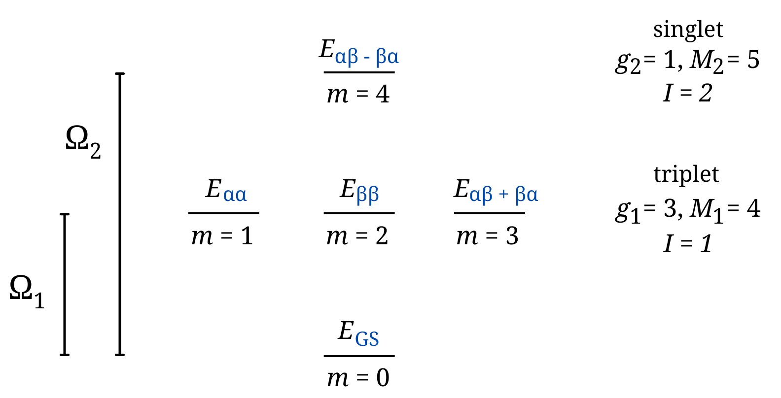
Figure 1: Diagram of the multiplet structure for the ensemble of interacting particles for a PIB, obeying spin symmetry. $I=1$ corresponds to the bi-ensemble, which includes up to $m=3$ (1st multiplet). $I=2$ corresponds to the tri-ensemble, which includes up to $m=4$ (2nd multiplet). The degeneracy of the highest multiplet included in the ensemble is given by the corresponding value of $g_{I}$, and $M_{I}$ is the total number of states included in the $I$th ensemble. The assignment of $m$’s within a multiplet are arbitrary.

II.3 Approximations to Hartree, Exchange, and Correlation

The development of accurate weight-dependent density-functional approximations (DFAs) for EDFT is an ongoing challenge. Existing ensemble approximations to $E_{xc}^{w}$ include the quasi-local-density approximation (qLDA) functional,Gross, Oliveira, and Kohn (1988c); Kohn (1986) the “ghost”-corrected exact exchange (EXX) functional,Nagy (1998); Gidopoulos, Papaconstantinou, and Gross (2002) the exact ensemble exchange functional (EEXX),Nagy (1995) a local system-dependent and excitation-specific ensemble exchange functional for double-excitations (CC-S),Marut et al. (2020) a universal weight-dependent local correlation functional (eVWN5) based on finite UEGs, Marut et al. (2020) and the orbital-dependent second-order perturbative approximation (PT2) for the ensemble correlation energy functional.Yang (2021) As noted in all the aforementioned works, ensemble HXC has special complications beyond those of GS DFT, such as the consideration that ensemble Hartree and exchange are not naturally separated in EDFT.Gould, Stefanucci, and Pittalis (2020) Though each of these approaches above to approximating ensemble XC energies provides insight into the necessary characteristics of ensemble DFAs, it is unclear whether any of them are appropriate for periodic systems since they were developed for localized systems. In this work, for a first exploration of EDFT on periodic systems, we choose a simple approximation based on a Local Spin Density Approximation (LSDA).

The “traditional” DFAs of GS DFT can be used for ensembles by evaluating them on ensemble densities:

$$E_{\text{Hxc}}^{\text{trad}}[\rho^{w}]=E_{\text{Hxc}}\bigg{[}\sum_{m=0}^{M_{I}-1}\mathtt{w}_{m}\rho_{\textit{m}}(r)\bigg{]}.$$ (18)

This use of the ensemble density with GS DFAs, typically only applied to Hartree and exchange, has been called “Ansatz 1.”Gould, Stefanucci, and Pittalis (2020) The use of ensemble densities in “traditional” GS DFAs results in fictitious interactions of ground- and excited-state densities, or “ghost interaction errors” (GIEs), in both Hartree and exchange which do not cancel each other. Gould, Stefanucci, and Pittalis (2020); Gidopoulos, Papaconstantinou, and Gross (2002); Pastorczak and Pernal (2014); Gross, Oliveira, and Kohn (1988c); Pribram-Jones et al. (2014) Additionally, with this form of ensemble DFA, the functional derivatives in equation (17) become zero, since the weight dependence is within the ensemble density only. As such, nothing is learned from application of EDFT in such an approximation. We instead opt to use ensemble-generalized LSDA, in which we build an ensemble average by evaluating the GS Hartree and LSDA functionals on the density of each state in the ensemble individually:

$$E_{\text{Hxc},\textit{w}}^{\text{LSDA}}[\rho]=\sum_{m=0}^{M_{I}-1}\mathtt{w}_{m}E_{\text{Hxc}}^{\text{LSDA}}[\rho_{\textit{m}}(r)],$$ (19)

which has been called “Ansatz 2.”Gould, Stefanucci, and Pittalis (2020) In this way, we ensure the ensemble functionals to be weight-dependent, giving us nonzero corrections in equation (17).

Derivatives of this equation with respect to $\mathtt{w}$ depend on the weights defined in equation (15), which in turn are determined by the multiplet structure and $I$, e.g., whether a bi-ensemble or tri-ensemble is used (figure 1), and have the general form:

$$\left.\frac{\partial E^{\text{LSDA,w}}_{\text{Hxc}}[\rho]}{\partial w_{I}}\right|_{\rho^{w}=\rho^{w}_{I}}=-\frac{g_{I}}{M_{I}-g_{I}}\sum_{m=0}^{M_{I}-g_{I}-1}E_{\text{Hxc}}[\rho_{\textit{m}}(r)]\\ +\sum_{m=M_{I}-g_{I}}^{M_{I}-1}E_{\text{Hxc}}[\rho_{\textit{m}}(r)]$$ (20)

Note a useful property: the sum of the coefficients of the $M_{I}$ states is

$$-\frac{g_{I}}{M_{I}-g_{I}}\left(M_{I}-g_{I}\right)+\left(1\right)g_{I}=1-1=0.$$ (21)

This property is essential allow the excitation energy be intensive (size-consistent) as we approach the thermodynamic limit, since individual total energy terms are extensive and grow without bound.

This definition of ensemble-generalized Hartree is GIE-free.Pribram-Jones et al. (2014) Though this choice avoids a significant source of GIE, our current form of ensemble-generalized LSDA does introduce some GIE from XC.Gould, Stefanucci, and Pittalis (2020) We report results for ensemble corrections which have been built using the weight-dependent Hartree of equation (19), denoted by HXC, and also for the case where there is no Hartree contribution to the correction, denoted by XC, due to the “traditional” Hartree definition in equation (18).

II.4 Densities of Ground and Excited States

Here we show explicitly the spin-polarized densities involved in the ground and excited states which we use in our EDFT calculations. All densities involved here include a contribution from the closed shell,

$$\rho_{\rm closed}(r)=\sum^{N_{e}/2-1}_{n=1}|\phi_{n}(r)|^{2}\left(|\alpha(\omega)|^{2}+|\beta(\omega)|^{2}\right),$$ (22)

and the ground-state density is

$$\rho_{\rm GS}(r)=\left|\phi_{1}(x)\right|\left(\left|\alpha(\omega)\right|^{2}+\left|\beta(\omega)\right|^{2}\right)+\rho_{\rm closed}(r),$$ (23)

where $\phi_{1}$ is the highest occupied state.

In the spin-polarized PIB system of even $N_{e}$, based on spin symmetry, the system has a nondegenerate GS, a triplet first excited state, and a singlet second excited state, as depicted in figure 1. An odd number of $N_{e}$ would result in a different multiplet structure, but we do not investigate that case here, since odd/even distinctions should disappear in the thermodynamic limit anyway. The density of the $\alpha\alpha$ state ($m_{s}=1$) in the triplet, obtained from its Slater determinant and then written in terms of its constituent wavefunctions, is:

$$\rho_{\alpha\alpha}(r)=\left|\phi_{1}(x)\alpha(\omega)\right|^{2}+\left|\phi_{2}(x)\alpha(\omega)\right|^{2}+\rho_{\rm closed}(r),$$ (24)

where $\phi_{2}$ is the lowest unoccupied state, with reference to the ground state. Then, for the $\beta\beta$ ($m_{s}=-1$) state in the triplet, we obtain a similar equation where the $\alpha$ spins are flipped to $\beta$ spins:

$$\rho_{\beta\beta}(r)=\left|\phi_{1}(x)\beta(\omega)\right|^{2}+\left|\phi_{2}(x)\beta(\omega)\right|^{2}+\rho_{\rm closed}(r).$$ (25)

While $\rho_{\alpha\alpha}(r)\neq\rho_{\beta\beta}(r)$, our approximations to the energy-density functional, evaluated on these two densities, yields the same numerical result for their energies as required by symmetry, and is the result obtained from any LSDA. For the $m_{s}=0$ excited states, we must use linear combinations of two Slater determinants to obtain the density:

$$\rho_{\alpha\beta\pm\beta\alpha}({r})=\frac{1}{2}\bigg{(}|\phi_{1}(x)\alpha(\omega)|^{2}+|\phi_{1}(x)\beta(\omega)|^{2}+\\ |\phi_{2}(x)\alpha(\omega)|^{2}+|\phi_{2}(x)\beta(\omega)|^{2}\bigg{)}+\rho_{\rm closed}(r).$$ (26)

We obtain the same density for the symmetric triplet ($+$) and antisymmetric singlet ($-$) sum of the two Slater determinants. No pure density functional can tell the two states, having identical densities, apart, despite the fact that the triplet should be degenerate with the other two triplet states.

We will consider later, in sections III.2 and III.3, two approaches to treating the triplet energy. The first method, outlined in III.3, is the symmetry-broken tri-ensemble, in which the correct densities for each state in the triplet, obtained from equations (24), (25), and (26), are used. Although $E_{\rm xc}[\rho_{\alpha\alpha}]$ and $E_{\rm xc}[\rho_{\beta\beta}]$ are equal, the energy $E_{\rm xc}[\rho_{\alpha\beta+\beta\alpha}]$ of the third member of the triplet has a higher energy, with their difference decreasing asymptotically towards 0 as $N_{e}\rightarrow\infty$. To address this issue, we have also considered the symmetry-enforced tri-ensemble in section III.2, in which we do not use the computed value of $E[\rho_{\alpha\beta+\beta\alpha}]$ at all, and instead use the value of $E[\rho_{\alpha\alpha}]=E[\rho_{\beta\beta}]$ to represent all three states, maintaining the degeneracy of the KS states forming the spin triplet. Since both the singlet and triplet ($m_{s}=0$) states have the same density, we write $\rho_{\alpha\beta\pm\beta\alpha}$ in sections II.5, III.2, and III.3 to refer to their shared density.

GOK ensemble theory requires that states are ordered based on the energies of the interacting system, and that all states from the GS up to and including the $I$th multiplet are included in the ensemble. It is not always practically feasible to be certain that there are no additional states lying between those we have included in the system,Marut et al. (2020) but we work under the assumption that we have included all states between the ground state and $I$th excited state, such that we have not violated the rules of the GOK ensemble.

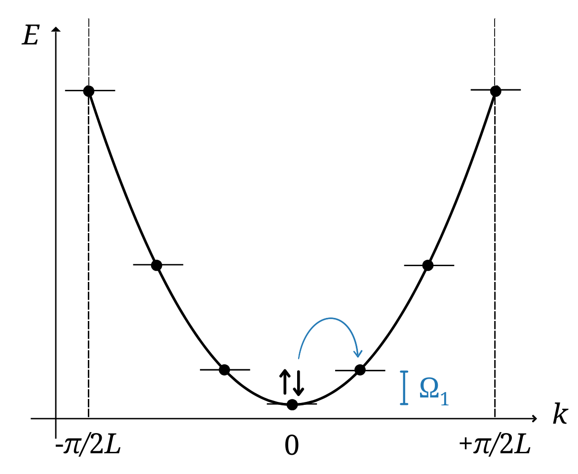
Figure 2: Band structure of the free electron gas, shown with a discrete set of 6 $k$-points in a Brillouin zone based on a periodic length $2L$. Arrow depicts an excitation with $\Delta k>0$.

II.5 1D Uniform Electron Gas

We first consider a possible way that a periodic system, could be discretized to allow application of EDFT. Leaving aside the question of whether such an approach is theoretically sound, we find that in the case of the UEG (the limit of our model) corrections to the KS excitation energies are identically zero, demonstrating that alternate strategies are needed in order to obtain non-trivial results.

We consider an infinite limit of our system in which the KS potential is zero everywhere, and periodic boundary conditions $\phi(x+2L)=\phi(x)$ are imposed for an arbitrary repeating cell of length $2L$. The KS wavefunctions have the form

$$\phi_{k}(x)=\sqrt{\frac{1}{2L}}e^{ikx},$$ (27)

and the KS energies for such a 1D system are

$$E=\frac{\hbar^{2}k^{2}}{2m_{e}},$$ (28)

as discussed further in section IV.3.

This system has a continuous spectrum of states and, as noted earlier, EDFT has been defined only for a discrete spectrum. We artificially discretize by choosing a set of $k$-points such as $k=(n/3)(\pi/2L)$ where $n=\left\{0,\pm 1,\pm 2,3\right\}$. We consider an excitation with $\Delta k>0$, to keep things simple and involve only one excited KS energy level, though this does bend the rules of the GOK EDFT. With the two KS energy levels, we obtain a singlet-triplet structure which is the same as in our finite well with even $N_{e}$ (Section II.1 and figure 1). We can then use the same form for the functional derivative terms to calculate the first excitation energy as before, equation (30). Filling the system with 2 electrons per cell of $2L$ results in two electrons in the lowest $k$-point, as in figure 2. With two electrons per unit cell, moving an electron from one $k$-point to the next represents exciting $1/2$ of all electrons in the periodic system. All of the ground- and excited-state densities are constant; e.g. from equation (24) we obtain:

$$\rho_{\alpha\alpha}(r)=\bigg{|}\sqrt{\frac{1}{2L}}e^{ik_{1}x}\alpha(\omega)\bigg{|}^{2}+\bigg{|}\sqrt{\frac{1}{2L}}e^{ik_{2}x}\alpha(\omega)\bigg{|}^{2}=\frac{1}{L},$$ (29)

where $k_{2}=k_{1}+\Delta k$. We find the same result for the three states which make up the triplet of the first excited state, equations (26), (24), and (25), and for the GS. The energy correction, as will be derived in detail in Section III.1, is

$$\left.\frac{\partial E_{\text{Hxc}}^{w}[\rho]}{\partial w_{I}}\right|_{\rho^{w}=\rho^{w}_{I}}=-3E_{\text{Hxc}}[\rho_{\text{GS}}]+E_{\text{Hxc}}[\rho_{\alpha\alpha}]\\ +E_{\text{Hxc}}[\rho_{\beta\beta}]+E_{\text{Hxc}}[\rho_{\alpha\beta\pm\beta\alpha}]=0,$$ (30)

where each density is identical, and the total correction goes to zero because the coefficients in front of each energy term always sum to zero (equation 21). Since the GOK ensemble correction depends on the ensemble density defined in equation (12), and each state has the same density, it is not possible to obtain a non-zero correction from EDFT to the UEG in this manner. Changing the number of electrons, number of $k$-points, length of the box, or which excitation we calculate (e.g. including $\Delta k<0$) would change the complexity for this model, but not the basic conclusion. We instead study a finite system which increases in size towards the thermodynamic limit to gain information about the behavior of EDFT’s correction as it approaches a periodic system.

II.6 Thermodynamic Limit of the Finite-Length Well

We increase the number of electrons in our system along with the length of the box, holding the average density constant:

$$\frac{N_{e}}{2L}=0.5\ \text{\AA}^{-1}\hskip 30.00005ptN_{e},L\rightarrow\infty.$$ (31)

As $N_{e}\rightarrow\infty$, a region of increasingly constant density begins to form at the center of the box, with decreasing oscillations and decreasing edge regions. According to the Wentzel–Kramers–Brillouin (WKB) Approximation, there will always be a peak at the classical turning points,Sakurai and Napolitano (2020) i.e. the edges of the box. As both $N_{e}$ and $L$ approach infinity, the density of the system becomes more uniform, with the nonuniform edge regions decreasing in width. To quantify this property (figure3), we first find the height $\rho^{\text{max}}$ of the highest peak within $-L\leq x\leq 0$. We average the values of the peaks and troughs of the density at the center ($x=0$) to find the average uniform density $\rho^{\text{uniform}}$. We then define $\Delta\rho^{\text{max}}=\rho^{\text{max}}-\rho^{\text{uniform}}$. Next, we consider an envelope function that excludes the oscillations of the density by linearly connecting the peaks of the density. We determine the width $\Delta x$ of the region between the edge of the box and the position at which the envelope has decreased to $\Delta\rho^{\text{max}}/e$ measured from $\rho^{\text{uniform}}$. We note that $\Delta x$ decreases not only as a fraction of $L$ but also in absolute terms, demonstrating that our model becomes increasingly uniform with increasing $L$ and that edge effects become negligible (figure 4). In this way, our model systems in the approach to the thermodynamic limit can be used to study how EDFT performs in a uniform periodic system.

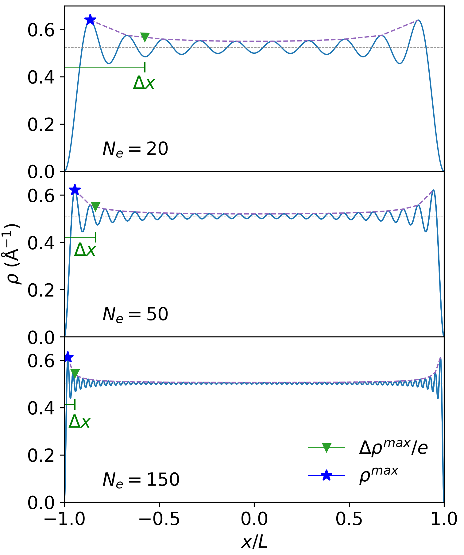
Figure 3: The non-interacting ensemble densities for $N_{e}=20$, $N_{e}=50$, and $N_{e}=150$, with interpolation line (dashed) between peaks. The maximum of the density within $-L\leq x\leq 0$ is $\rho^{\text{max}}$. The average density at the center of the box is shown as a dotted horizontal line. The width of the edge region, $\Delta x$, is defined as the width from the edge of the box to the point at which the interpolation line is $\Delta\rho^{\max}/e$ from the center peak-to-peak amplitude average, as described in section II.6. The width of $\Delta x$ spans a smaller portion of the box as $N_{e}$ increases.

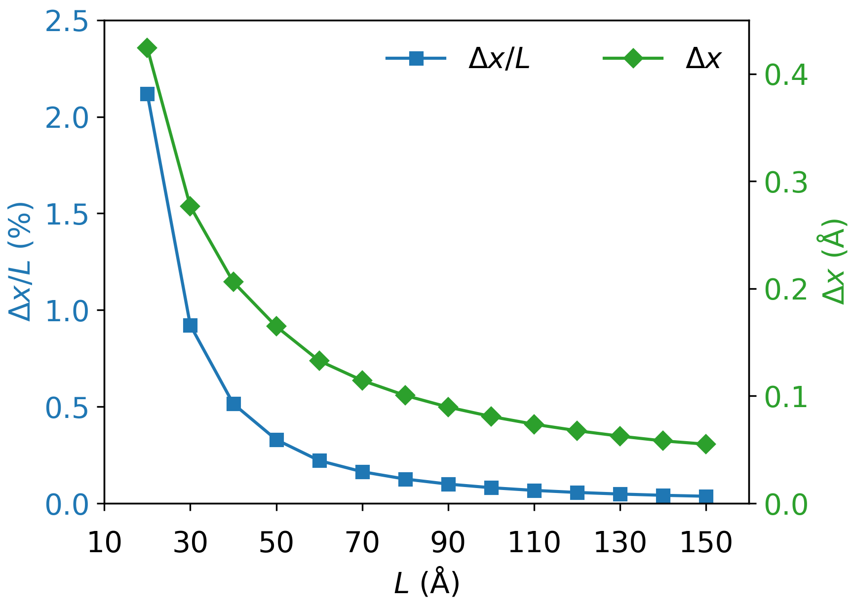
Figure 4: Decreasing width of the edge regions of the density, with increasing $L$. The average density is held constant to 0.5 $\text{\AA}^{-1}$ as in equation (31). The right axis is the width of the region $\Delta x$, and the left axis is the percentage of the half-length of the box spanned by $\Delta x$.

III Computational Methodology

Octopus is uniquely suited for this work due to its ability to define arbitrary potentials and therefore easily treat model systems and 1D systems.Andrade et al. (2015); Tancogne-Dejean et al. (2020) In this work we use Octopus version 11.4. In order to realize our condition of setting the KS potential equal to the 1D finite well potential in Octopus, the potential is set to zero within a finite domain determined by $L$. The wavefunction is constrained to zero at the boundaries of the box. We limit our system to an even number of electrons $N_{e}$ whose ratio to $L$ is held fixed as in equation (31), and consider its spin-polarized solutions obtained from the PIB as in equations (5) and (7). The average density of 0.5 $\text{\AA}^{\scalebox{0.75}[1.0]{$-$}1}$ was used to achieve convergence since systems with the larger average density of 1 $\text{\AA}^{\scalebox{0.75}[1.0]{$-$}1}$ were unable to be converged for all values of $N_{e}$. The starting initial guess in the Kohn-Sham equations are random wavefunctions. We set an eigensolver tolerance of $10^{-6}$ eV, which can require up to 1000 eigensolver iterations, and do not use a preconditioner. Eigensolver convergence was difficult to achieve and we settled on this fixed density ratio, grid, and eigensolver type which gave adequate convergence behavior. A grid spacing of 0.01 Å is used for all calculations in order to converge energies to within 0.05 eV of the analytic solutions of the PIB. Though the KS eigenvalues and eigenfunctions can be obtained analytically, we use the values obtained from Octopus for consistency in comparing to the ensemble-generalized LSDA HXC values which we obtain from Octopus.

For each choice of $N_{e}$, we first run a spin-polarized GS calculation for independent particles in 1D, calculating $N_{e}/2+1$ states to include all the filled states plus one unoccupied state. We then run a “one-shot” DFT calculation with the same value of $N_{e}$, but occupations of the KS states for each state in the ensemble are built based on $f^{m}_{j}$ of equation (12), which are obtained from Slater determinants as outlined in section II.4. These calculations use fixed wavefunctions from the previous independent-particles calculation, and provide $E_{\rm H}$, $E_{\rm x}$, and $E_{\rm c}$ for a density built from the given occupations.

Given the problematic nature of the Coulomb interaction in 1D, we describe the electron-electron interactions with the 1D soft Coulomb potential, where we set the softening parameter, $a$, to 1 Bohr radius ($a_{0}$):

$$v_{\text{sc}}(x)=\frac{1}{\sqrt{x^{2}+a^{2}}}.$$ (32)

We use the 1D LSDA exchangeHelbig et al. (2011) and correlation functionalsCasula, Sorella, and Senatore (2006) as implemented in libxc Lehtola et al. (2018), which were parametrized for this interaction and value of $a$.

III.1 Bi-ensemble

Starting from equation (19), the GOK weighting scheme from equation (15), and the multiplet structure of figure 1A with a choice of the bi-ensemble ($I=1$, $g_{1}=3$ and $M_{1}=4$), our weights are:

$$\mathtt{w}_{m}=\begin{cases}1-3\mathtt{w}&m<1,\\ \mathtt{w}&m\geq 1.\end{cases}$$ (33)

With our earlier choice of ensemble-generalized LSDA in equation (19), and relying on the GOK weight definition in equation (15), the energy functional is:

$$E_{\text{Hxc}}^{w}[\rho]=\left(1-3\mathtt{w}\right)(E_{\text{Hxc}}[\rho_{\text{GS}}])+\mathtt{w}(E_{\text{Hxc}}[\rho_{\alpha\alpha}]\\ +E_{\text{Hxc}}[\rho_{\beta\beta}]+E_{\text{Hxc}}[\rho_{\alpha\beta+\beta\alpha}]).$$ (34)

The corresponding energy correction, as in equation (30), is

$$\left.\frac{\partial E_{\text{Hxc}}^{w}[\rho]}{\partial w_{I}}\right|_{\rho^{w}=\rho^{w}_{I}}=-3E_{\text{Hxc}}[\rho_{\text{GS}}]+E_{\text{Hxc}}[\rho_{\alpha\alpha}]\\ +E_{\text{Hxc}}[\rho_{\beta\beta}]+E_{\text{Hxc}}[\rho_{\alpha\beta\pm\beta\alpha}],$$ (35)

If we rewrite this equation using our knowledge of the system, that is, that the GS is singly degenerate and the first excited state is triply degenerate so that $E_{\text{Hxc}}[\rho_{\alpha\alpha}]=E_{\text{Hxc}}[\rho_{\beta\beta}]=E_{\text{Hxc}}[\rho_{\alpha\beta+\beta\alpha}]$, then we can write the equation as:

$$\frac{\partial E_{\text{Hxc}}^{w}[\rho]}{\partial\mathtt{w}}\bigg{\rvert}_{\rho=\rho^{w}}=-3E_{\text{Hxc}}[\rho_{\text{GS}}]+3E_{\text{Hxc}}[\rho_{\alpha\alpha}].$$ (36)

Revisiting equation (17), it becomes apparent that the difference of KS energies $E_{I}-E_{0}$ can be reduced to a difference of eigenvalues via equation (13):

$$E_{I}-E_{0}=\sum^{\infty}_{j=1}f^{I}_{j}\epsilon_{j}-\sum^{\infty}_{j=1}f^{0}_{j}\epsilon_{j}.$$ (37)

This expression reduces to the same result for both the bi-ensemble ($I=1$) and the tri-ensemble ($I=2$) – anticipating the next section – that is, $E_{2}-E_{0}=E_{1}-E_{0}=\epsilon_{n=2}-\epsilon_{n=1}$. To calculate the excitation energy $\Omega_{I}$ of equation (17), we still must calculate the third term, the derivative of the HXC functional with respect to the weight. Combined with equation (37), equation (17) reduces to:

$$\Omega_{1}=\epsilon_{n=2}-\epsilon_{n=1}-3E_{\text{Hxc}}[\rho_{\text{GS}}]+3E_{\text{Hxc}}[\rho_{\alpha\alpha}].$$ (38)

Figure 5: Ensemble-corrected first excitation energies compared to KS energy differences for: (a) the triplet $\Omega_{1}$ of the bi-ensemble described in section III.1 and by equation (38), where $\Omega_{1}$ (XC) has been scaled up by 5, and (b) the singlet $\Omega_{1}^{\text{flip}}$ of the flipped bi-ensemble, described in section IV.1 and by equation (45). In (b) the KS difference of energies, $E_{0}\scalebox{0.75}[1.0]{$-$}E_{1}$, has been scaled up by $10^{3}$. Insets show the relative ordering of the first excited state and ground state for each ensemble. HXC denotes results with a weight-dependent Hartree, while XC denotes the use of a “traditional” Hartree, as explained in section II.3.

III.2 Tri-ensemble: Symmetry-Enforced

We now consider a tri-ensemble, $I=2$, based on figure 1. In order to calculate the singlet energy, $\Omega_{2}$, we begin with equation (17). Knowing the difference of non-interacting energies from the PIB, all that is left is to calculate the derivative of $E_{\text{Hxc}}$. Given the multiplet structure of figure 1A with $g_{2}=1$ and $M_{2}=5$, we have weights

$$\mathtt{w}_{m}=\begin{cases}\frac{1-\mathtt{w}}{4}&m<4,\\ \mathtt{w}&m\geq 4.\end{cases}$$ (39)

We obtain the general form for the functional derivative with respect to the weight:

$$\left.\frac{\partial E_{\text{Hxc}}^{w}[\rho]}{\partial\mathtt{w}}\right|_{\rho=\rho^{w}}=-\frac{1}{4}(E_{\text{Hxc}}[\rho_{\text{GS}}]+E_{\text{Hxc}}[\rho_{\alpha\alpha}]\\ +E_{\text{Hxc}}[\rho_{\beta\beta}]+E_{\text{Hxc}}[\rho_{\alpha\beta+\beta\alpha}])+E_{\text{Hxc}}[\rho_{\alpha\beta-\beta\alpha}].$$ (40)

To use this expression directly would break the spin-symmetry of the triplet, as noted in Section II.4. We note that other EDFT methods have avoided this symmetry-breaking issue via approximations based on multi-determinant spin eigenstates rather than just the density.Pribram-Jones et al. (2014) To enforce spin symmetry, we use the energy $E_{\text{Hxc}}[\rho_{\alpha\alpha}]$ for all states in the triplet. The last term, representing the singlet, we write as $E_{\text{Hxc}}[\rho_{\alpha\beta\pm\beta\alpha}]$. The second excitation energy (i.e. the singlet), denoted $\Omega_{2}^{\text{e}}$ with $e$ for symmetry-enforced approach, then is calculated as:

$$\Omega_{2}^{\text{e}}=\epsilon_{n=2}-\epsilon_{n=1}-\frac{1}{4}E_{\text{Hxc}}[\rho_{\text{GS}}]-\frac{3}{4}E_{\text{Hxc}}[\rho_{\alpha\alpha}]+\\ E_{\text{Hxc}}[\rho_{\alpha\beta\pm\beta\alpha}].$$ (41)

Figure 6: Energy of singlet states obtained as second excitation energies $\Omega_{2}$ from the tri-ensemble compared to KS energy differences $E_{0}\scalebox{0.75}[1.0]{$-$}E_{1}$ using (a) the symmetry-enforced tri-ensembles described in section III.2 and by equation (41), and (b) the symmetry-broken tri-ensemble described in section III.3 and by equation (42). Insets show detail of regions for small $N_{e}$. HXC denotes results with a weight-dependent Hartree, while XC denotes the use of a “traditional” Hartree, as explained in section II.3.

Table 1: Ensemble-corrected excitation energies tabulated versus number of electrons $N_{e}$, compared with KS energy difference $E_{1}-E_{0}$, all reported in eV. $\Omega_{1}$ and $\Omega_{1}^{\text{flip}}$ are the first excitation energies of the bi-ensemble (energy of triplet) and flipped bi-ensemble (energy of closed-shell singlet), respectively. $\Omega_{2}^{e}$ and $\Omega_{2}^{b}$ are the second excitation energies, corresponding to the open-shell singlet, obtained from the symmetry-enforced and symmetry-broken tri-ensembles, respectively. HXC denotes results with a weight-dependent Hartree, while XC denotes the use of a “traditional” Hartree, as explained in section II.3.

		$\Omega_{1}$		$\Omega^{\text{flip}}_{1}$		$\Omega^{\text{e}}_{2}$		$\Omega^{b}_{2}$
$N_{e}$	$E_{1}-E_{0}$	XC	HXC	XC	HXC	XC	HXC	XC	HXC
2	6.988	$0.2471$	$-10.29$	$\scalebox{0.75}[1.0]{$-$}59.68$	$19.06$	9.369	8.491	8.633	7.755
4	2.925	$0.3339$	$-$ 4.119	$\scalebox{0.75}[1.0]{$-$}93.76$	$122.2$	3.949	3.578	3.639	3.268
6	1.822	$0.2493$	$-$ 2.454	$\scalebox{0.75}[1.0]{$-$}133.8$	230.6	2.469	2.244	2.275	2.049
8	1.319	$0.1687$	$-$ 1.741	$\scalebox{0.75}[1.0]{$-$}174.9$	347.9	1.797	1.638	1.653	1.494
10	1.032	0.1161	$\scalebox{0.75}[1.0]{$-$}1.350$	$-$ 216.4	$472.9$	1.413	1.291	1.299	1.177
20	0.4931	0.0253	$\scalebox{0.75}[1.0]{$-$}0.6384$	$-$ 425.9	$1182$	0.6846	0.6293	0.6270	0.5717
30	0.3236	0.0065	$\scalebox{0.75}[1.0]{$-$}0.4189$	$-$ 635.9	$1985$	0.4520	0.4165	0.4133	0.3778
40	0.2408	0.0005	$\scalebox{0.75}[1.0]{$-$}0.3119$	$-$ 846.1	$2851$	0.3374	0.3114	0.3083	0.2822
50	0.1917	$-$ 0.0018	$\scalebox{0.75}[1.0]{$-$}0.2485$	$-$ 1056	$3764$	0.3374	0.2486	0.2458	0.2252
150	0.0631	$-$ 0.0027	$\scalebox{0.75}[1.0]{$-$}0.0817$	$-$ 3159	$14320$	0.0891	0.0825	0.0812	0.0746

III.3 Tri-ensemble: Symmetry-Broken

In a second alternative method, we do not enforce any symmetry, and only simplify equation 40 based on equalities that are satisfied in practice by LSDA. We use $E_{\text{Hxc}}[\rho_{\alpha\alpha}]$ for only two states in the triplet. $E_{\text{Hxc}}[\rho_{\alpha\beta\pm\beta\alpha}]$ is then used for the third state of the triplet and for the singlet state, resulting in an ensemble with broken spin-symmetry. The second excitation energy, denoted $\Omega_{2}^{\text{b}}$ with $b$ for symmetry-broken approach, then is calculated as:

$$\Omega_{2}^{\text{b}}=\epsilon_{n=2}-\epsilon_{n=1}-\frac{1}{4}E_{\text{Hxc}}[\rho_{\text{GS}}]-\frac{1}{2}E_{\text{Hxc}}[\rho_{\alpha\alpha}]\\ +\frac{3}{4}E_{\text{Hxc}}[\rho_{\alpha\beta\pm\beta\alpha}].$$ (42)

The difference between corrected energies obtained from the symmetry-enforced and symmetry-broken ensembles is

$$\Omega_{2}^{\text{e}}-\Omega_{2}^{\text{b}}=-\frac{1}{4}E_{\text{xc}}[\rho_{\alpha\alpha}]+\frac{1}{4}E_{\text{xc}}[\rho_{\alpha\beta\pm\beta\alpha}].$$ (43)

Because the Hartree term is spin-independent, its value is the same when evaluated on $\rho_{\alpha\alpha}$ and $\rho_{\alpha\beta\pm\beta\alpha}$. For this reason, the difference in corrected excitation energies obtained in equation (43) only has a contribution from XC, and is the same whether an ensemble-generalized Hartree is used or not.

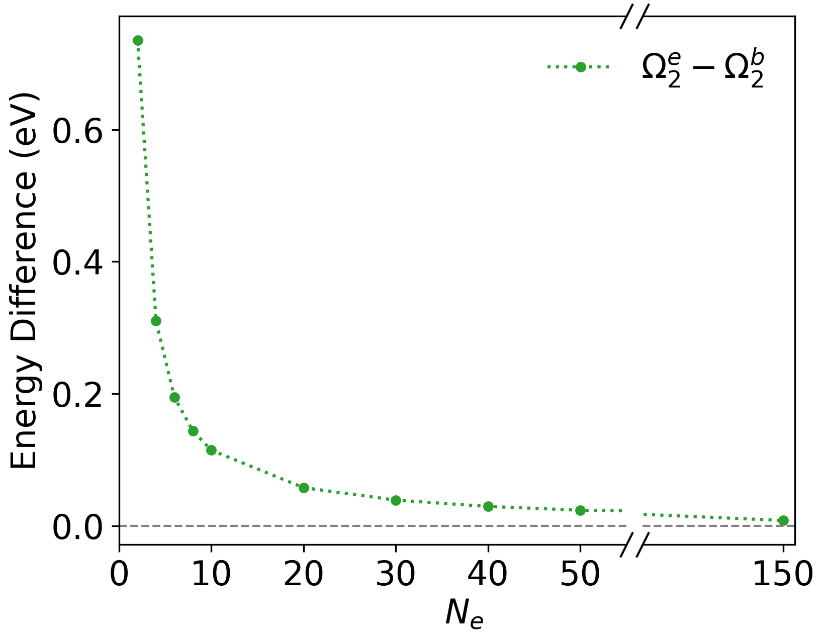
Figure 7: Difference between energy of singlet excited states from the symmetry-enforced ($\Omega^{e}_{2}$) and symmetry-broken ($\Omega^{b}_{2}$) tri-ensembles, as given in equation (43).

IV Results and Discussion

IV.1 Bi-ensemble and Triplet Instability

The corrected first excitation energies $\Omega_{1}$ from the bi-ensemble are shown in figure 5a. With the ensemble-generalized LSDA HXC functional, $\Omega_{1}$ is negative, which indicates that the energy of the triplet is beneath the ground state, and the triplet is unstable in this theory. When a “traditional” Hartree DFA is used (the XC case), the ensemble-corrected triplet energies are positive for $N_{e}\leq 40$, above which which the triplet is unstable. These XC excitation energies are one order of magnitude smaller than the KS difference in energies. We note that finding a multiplet ordering different from the one assumed in construction of our ensemble means that the construction was invalid according to the rules of GOK EDFT, although this re-ordering is not a problem according to a more general EDFT definition in which weights must be monotonically non-increasing with energy only within a given symmetry.Gould and Pittalis (2020)

To investigate the triplet instability further, and attempt to correct our ensemble construction, we consider the possibility that the true system should have a triplet GS and a singlet first excited state, as suggested by the negative triplet excitation energy. The weighting scheme of this flipped system is:

$$\mathtt{w}_{m}=\begin{cases}\frac{1-\mathtt{w}}{3}&m<3,\\ \mathtt{w}&m\geq 3.\end{cases}$$ (44)

This weighting provides an ensemble-corrected excitation energy from this triplet GS to the singlet:

$$\Omega_{1}^{\text{flip}}=E_{0}-E_{1}+E_{\text{Hxc}}[\rho_{\alpha\alpha}]-E_{\text{Hxc}}[\rho_{\text{GS}}].$$ (45)

We use $E_{\text{Hxc}}[\rho_{\alpha\alpha}]$ for the energy of all states in the triplet, as for the symmetry-enforced tri-ensemble (section III.1). We then treat $E_{\text{Hxc}}[\rho_{\text{GS}}]$ as the excited-state singlet. Triplet instabilities are known to exist in other theories, such as Hartree-Fock,Overhauser (1960); Sawada and Fukuda (1961); Lefebvre and Smeyers (1967) time-dependent Hartree-Fock (TDHF),Dreuw and Head-Gordon (2005); Čížek and Paldus (2004) and TDDFT.Peach and Tozer (2012) Triplet instabilities have also been reported in the electron gas at metallic densities.Lam (1971) Whether or not this instability is a failure of the theory or a true characteristic of this model is not clear. Regardless, EDFT in our approximations contradicts itself on the placement of the triplet in most cases. The triplet is unstable in the bi-ensemble when a weight-dependent Hartree is used, and stable until $N_{e}>40$ when a “traditional” Hartree is used, as shown in figure 5a. When the ensemble is flipped to attempt to address the instability, the triplet is pushed back above the closed-shell singlet when a “traditional” Hartree is used, and the singlet energy appear to be diverging toward $-\infty$. While the flipped ensemble with weight-dependent Hartree gives a positive excitation energy consist with the reordering of the ensemble into a triplet ground state, the excitation energy appears to diverge toward $+\infty$. These results are shown in figure 5b. Overall, we find serious pathologies in the bi-ensemble, and the divergences indicate an inapplicability to the thermodynamic limit.

IV.2 Singlet Excitations from Tri-ensembles

All singlet excitation energies from the tri-ensemble are positive (figure 6). For the symmetry-enforced tri-ensemble, the corrected second excitation energy $\Omega_{2}^{\text{e}}$ is greater in value than the KS second excitation energy $E_{1}\scalebox{0.75}[1.0]{$-$}E_{0}$, regardless of whether a weight-dependent Hartree is used or not. The weight-dependent Hartree contribution is negative, and it is on the order of 0.01 eV lower than the XC correction at $N_{e}=150$.

The symmetry-broken tri-ensemble provides a corrected second excitation energy $\Omega_{2}^{\text{b}}$ which is again greater in value than the KS energy difference, whether the Hartree term used is weight-dependent or not. The corrections are somewhat smaller than in the symmetry-enforced case. The weight-dependent Hartree contribution is identical to the symmetry-enforced case, as discussed above. We find that the excitation energy difference between symmetry-enforced and symmetry-broken approaches is always positive and monotonically decreasing, and is about an order of magnitude smaller than the excitation energies themselves (figure 7), indicating that this distinction does not have a major impact on the results.

IV.3 Effective Mass

Figure 8: Effective masses, calculated from equation (46), for (a) the bi-ensemble described in section III.1, (b) flipped bi-ensemble, described in section IV.1, (c) the symmetry-enforced tri-ensemble of section III.2, and (d) the symmetry-broken tri-ensemble of section III.3. In (b) a horizontal line is drawn at 0 and a vertical line marks the divergence around $N_{e}=41$. HXC denotes results with a weight-dependent Hartree, while XC denotes the use of a “traditional” Hartree, as explained in section II.3.

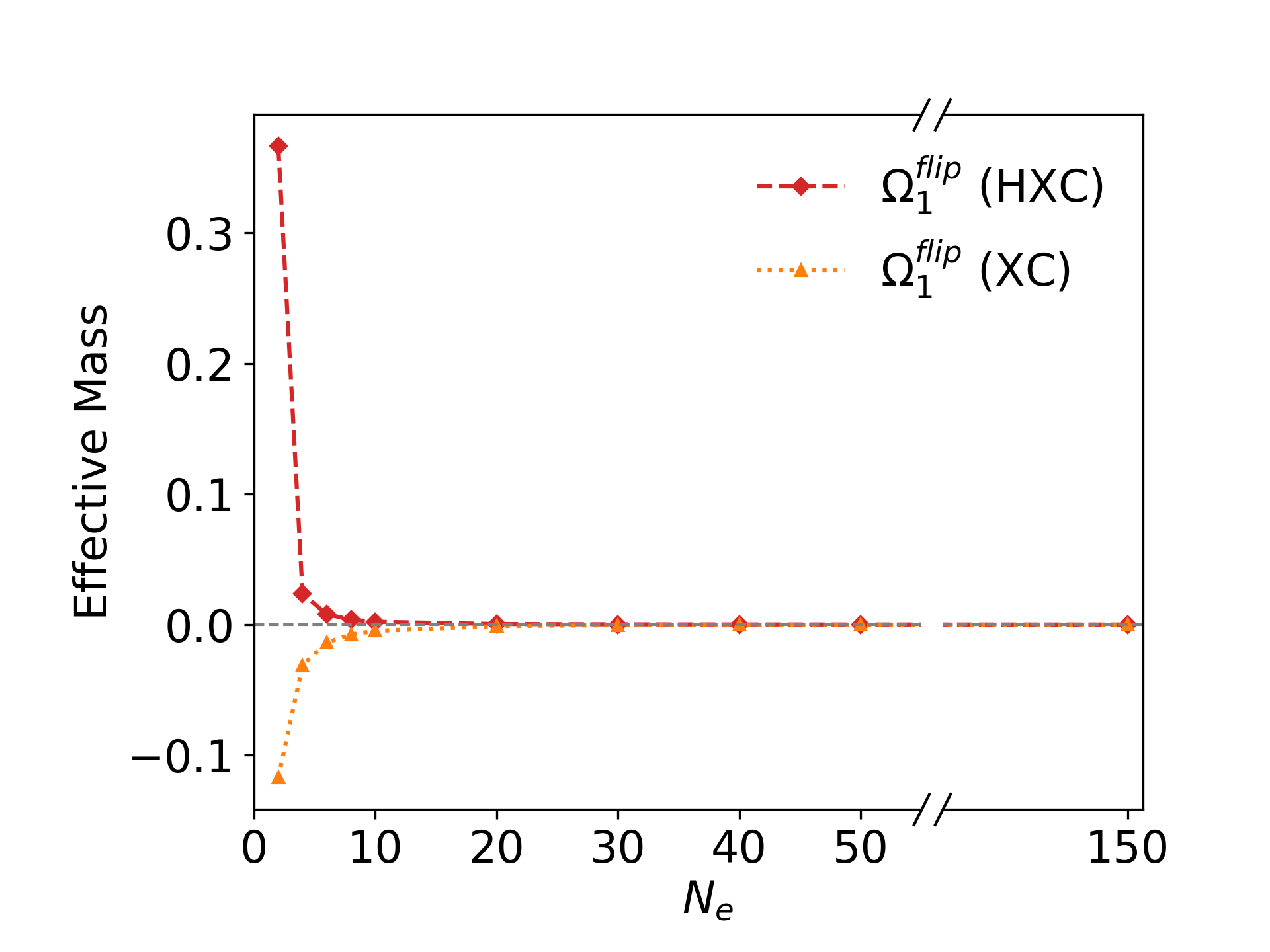
Figure 9: Effective mass, calculated from equation (46), for the flipped bi-ensemble described in section IV.1. HXC denotes results with a weight-dependent Hartree, while XC denotes the use of a “traditional” Hartree, as explained in section II.3.

The effective mass is a useful parameter by which to validate a model’s treatment of interactions, and it can be directly studied in real systems. For instance, many studies have tried to reproduce the experimentally measured occupied bandwidth of sodium, with varying success.Maezono et al. (2003); Puente, Serra, and Casas (1994); Fiolhais, Nogueira, and Marques (2003) To compute an effective mass in our case, we consider the excitation as an energy difference between $k$-points $k_{2}$ and $k_{1}$ on parabolic bands in a UEG, as in equation (28). We assume that the $k$-points for the excitation are the same for the non-interacting system and the interacting, ensemble-corrected system, which is appropriate if the Fermi level is not shifted with respect to the states by the interaction. This condition will be fulfilled if the EDFT scheme constitutes a conserving approximation.Baym and Kadanoff (1961) With these considerations, we obtain the effective mass as:

$$\frac{\Delta E^{\text{ip}}}{\Delta E^{\text{int}}}=\frac{E_{I}-E_{0}}{\Omega_{I}}=\frac{\frac{\hbar^{2}{k_{2}}^{2}}{2m_{e}}\scalebox{0.75}[1.0]{$-$}\frac{\hbar^{2}{k_{1}}^{2}}{2m_{e}}}{\frac{\hbar^{2}{k_{2}}^{2}}{2m^{\text{*}}}\scalebox{0.75}[1.0]{$-$}\frac{\hbar^{2}{k_{1}}^{2}}{2m^{\text{*}}}}=\frac{m^{\text{*}}}{m_{e}}.$$ (46)

While formally the effective mass is only defined for periodic systems, we study the limit of this ratio as our model approaches a periodic system. The effective masses at the thermodynamic limit (estimated as the results at our largest $N_{e}$, 150) are reported in Table 2. In each case, the electron mass ratio approaches a limit which differs from the bare mass, in which case $m^{*}/m=1$. By contrast, it can be shown analytically that GS DFT with LDA gives the effective mass in a UEG always equal to the free electron mass.Louie (2006) That a nontrivial change in the effective mass is found through EDFT shows the potential of EDFT for periodic systems, and for additional insight to be obtained through the use of more sophisticated ensemble DFAs.

Our results find monotonically decreasing effective masses with increasing system size for the tri-ensemble, while the effective masses for the bi-ensemble exhibit different behavior depending on whether or not a weight-dependent Hartree is used. For the bi-ensemble with weight-dependent Hartree, the effective mass decreases monotonically until $N_{e}=30$, at which point the effective mass increases as it approaches its limit of $-$ 0.7715, shown in figure 8a. With a “traditional” Hartree, the effective mass diverges near $N_{e}=41$ before approaching its value of $-$ 23.24 in the limit, as shown in figure 8b. In the flipped bi-ensemble, the effective mass approaches zero due to the divergence of $\Omega_{1}^{\text{flip}}$ towards $\pm\infty$ in the weight-dependent XC and HXC cases, respectively, illustrated in figure 9. The use of weight-dependent Hartree in the tri-ensemble results increases the ratio in the limit from 0.7080 to 0.7646 in the symmetry-enforced tri-ensemble, and from 0.7767 to 0.8452 in the symmetry-broken tri-ensemble, illustrated in figures 8c and 8d, respectively. In the case of the bi-ensemble, negative effective masses are found which are not remedied by re-construction of the ensemble with the ordering of the closed-shell singlet and triplet flipped.

While comparison to 1D values would be preferred, we are not aware of any reported values for the effective mass of electrons in the 1D UEG. The effective masses between 2D and 3D UEGs are known to differ, and it is possible that the 1D values may not be similar. However, it is reasonable to consider the 2D and 3D cases as points of comparison. We compare our results to the effective mass for the UEG obtained via Monte Carlo for 2D and 3D systems with density parameter $r_{s}\leq 4$, representing the metallic regime, where $r_{s}\leq 1$ $a_{0}$ represents the high-density regime.Haule and Chen (2022); Parr and Yang (1989) In the 3D case, effective masses in the UEG obtained by variational diagrammatic Monte Carlo (MC) have been found to be 0.955(1) for $r_{s}=1$ $a_{0}$, and 0.996(3) at $r_{s}=4$ $a_{0}$.Haule and Chen (2022) Other calculations on the 3D UEG done via diffusion MC extrapolated to the thermodynamic limit have reported an effective mass of 0.85 at $r_{s}\approx 4$ $a_{0}$.Azadi, Drummond, and Foulkes (2021) For ferromagnetic 2D UEGs at $r_{s}=1$ $a_{0}$, a value of 0.851(5) has been reported using diffusion MC.Drummond and Needs (2013) In the high-density limit for a 3D electron gas, the effective mass is expected to be less than one.Krakovsky and Percus (1996) Our 1D results fall outside the range of reported values for the 2D and 3D cases, though values for the tri-ensemble are all less than one, falling in line with this property of 3D results. The symmetry-broken tri-ensemble value namely 0.8452 is the value closest to those reported for 3D cases.

Table 2: Effective masses in the thermodynamic limit, estimated from $N_{e}=150$, obtained from equation (46) using the ensemble-corrected excitation energies. HXC denotes results with a weight-dependent Hartree, while XC denotes the use of a “traditional” Hartree, as explained in section II.3.

Excitation	HXC	XC
$\Omega_{1}$	$-$ 0.7715	$-$ 23.24
$\Omega_{1}^{\text{flip}}$	0.0005	$-$ 0.0022
$\Omega_{2}^{\text{e}}$	0.7646	0.7080
$\Omega_{2}^{\text{b}}$	0.8452	0.7767

V Conclusion

Since EDFT was designed for the treatment of discrete energy levels, it does not readily adapt to the band structure of solids. We have therefore instead approached the application of EDFT to a periodic system through a set of systems having the same fixed average density, and studied its approach to the thermodynamic limit. We have considered ensemble-corrected excitation energies for systems where the KS potential is set to the PIB potential, becoming the HEG in the thermodynamic limit, and avoiding the need for SCF calculations.

Corrections to the singlet energy obtained from a tri-ensemble are positive, increasing the KS energy differences. We find a triplet instability for the bi-ensemble case, which is not always reproduced if the ensemble is re-constructed with a triply degenerate GS. While EDFT provides nonzero corrections to excitation energies in the finite regime, in the approach to the thermodynamic limit, these approach zero. This approach towards zero is exhibited by the KS energy difference as well, and is expected for our metallic system.Kaxiras and Joannopoulos (2019) effective masses in the thermodynamic limit for each of the methods were calculated, and found to approach a positive limit in the tri-ensemble and a negative limit in the bi-ensemble, with the flipped case resulting in a ratio which diverges before approaching a negative value. A nontrivial change in the effective mass is found in the approach to the limit, even with a weight-dependent Hartree term derived from the GS Hartree and LSDA XC in the metallic system, indicating the potential for improvement in this theory through development of DFAs.

Prior work by Kraisler and KronikKraisler and Kronik (2013) examined the derivative discontinuity of XC functionals (which corrects the KS gap) in the thermodynamic limit, based on ensemble considerations (but not on EDFT per se). They note that the Hartree-based contribution to the missing derivative discontinuity vanishes in the thermodynamic limit, with the exact XC component being the source of a useful correction. They note that, as we see in our results, LDA-based corrections to the gap vanish due to known insufficiencies in this approximation. By contrast, our work by investigating effective masses as well, found that there can be a nontrivial correction from LDA in the thermodynamic limit.

We have investigated the impact of using two different forms of ensemble-generalized Hartree, one in which there is explicit weight dependence in the functional, which is then applied to densities of individual states, and one in which the weight-dependence is only accounted for in the ensemble density (the “traditional” Hartree). However, it is known that neither method treating the ensemble Hartree is sufficient to treat systems with “difficult” spin multiplets in finite systems.Gould, Stefanucci, and Pittalis (2020) In all cases we have used the former explicitly weight-dependent ensemble-generalized LDA XC. Given that neither LDA nor GGA in periodic systems exhibit the necessary divergence of $f_{xc}$,Onida, Reining, and Rubio (2002) it reasonable to expect that implementation of more sophisticated ensemble DFAs, particularly non-local and GIE-free XC, would be needed for fuller analysis of EDFT’s applicability and limitations in treating periodic systems.

While the treatment of increasingly large finite systems at a fixed average density may not be practical for extracting information about real systems, our results point to this approach being serviceable for periodic systems in EDFT, and could be developed further. Further study of these same systems in the thermodynamic limit can be extended to 2D and 3D, as well as to variable average density. The results of this method when applied to models with nonuniform potential, such as the Kronig-Penney model, and to systems with odd number of electrons may offer further insight.