Multistable Kuramoto splay states in a crystal of mode-locked laser pulses: Supplementary Material

I Motivation for the order parameter

In order to measure the degree of order in a train of pulses, it is instructive to introduce an order parameter. We consider for a configuration of $N$ pulses the first order correlation function

$$g^{\left(1\right)}\left(r\right) =\frac{\left\langle E^{*}\left(t\right)E\left(t+r\right)\right\rangle}{\left\langle\left|E\left(t\right)\right|^{2}\right\rangle}.$$ (1)

This function needs to be evaluated at the position of the neighboring pulse, i.e. when $N$ pulses are present in the cavity of size $\tau$, we consider $g^{\left(1\right)}\left(\frac{\tau}{N}\right)$. Further, the average is defined as

$$\left\langle E\left(t\right)\right\rangle=\frac{1}{\tau}\intop_{0}^{\tau}E\left(t\right)dt.$$ (2)

Experimentally, this makes sense as the first order correlation function can be obtained by interfering the electric field with itself after a retarded time $\frac{\tau}{N}$. Next, we consider the electric field to consist of $N$ identical in shape and equidistant pulses. This implies that there is no shape deformation mode. The equidistance of the pulses implies that the translation mode is damped. This is the case for pulses in a relatively short cavity, where pulses are locked in position due to gain repulsion as it is the case in the experiment presented in the main part of the paper. The remaining degree of freedom is the phase $\varphi_{j}$ of the $j$-th pulse such that the full field $E(t)$ reads

$$E\left(t\right)=\sum_{k=1}^{N}E_{0}\left(t-\left(k-1\right)\frac{\tau}{N}\right)e^{-i\varphi_{k}}\,,$$ (3)

where $E_{0}\left(t\right)$ is the optical field for a single pulse. Further, we define $\bar{I}\equiv\left\langle\left|E_{0}\left(t\right)\right|^{2}\right\rangle$ as the average intensity of a single pulse. The first order correlation function then reads

$$g^{\left(1\right)}\left(\frac{\tau}{N}\right) =\frac{\left\langle\left[\sum_{k=1}^{N}E_{0}^{*}\left(t-\left(k-1\right)\frac{\tau}{N}\right)e^{i\varphi_{k}}\right]\left[\sum_{k=1}^{N}E_{0}\left(t-k\frac{\tau}{N}\right)e^{-i\varphi_{k}}\right]\right\rangle}{\left\langle\left|\sum_{k=1}^{N}E_{0}\left(t-k\frac{\tau}{N}\right)e^{i\varphi_{k}}\right|^{2}\right\rangle}$$

$$=\frac{\left\langle\sum_{k=1}^{N}\left|E_{0}\left(t-k\frac{\tau}{N}\right)\right|^{2}e^{i\left(\varphi_{k+1}-\varphi_{k}\right)}\right\rangle}{N\bar{I}}$$ (4)

$$=\frac{\left\langle\left|E_{0}\left(t\right)\right|^{2}\right\rangle}{N\bar{I}}\sum_{k=1}^{N}e^{i\left(\varphi_{k+1}-\varphi_{k}\right)}$$

$$=\frac{1}{N}\sum_{k=1}^{N}e^{i\left(\varphi_{k+1}-\varphi_{k}\right)},$$

where we used the periodic boundaries, i.e. $E_{0}\left(t\right)=E_{0}\left(t-\tau\right)$ and considered the overlap of the pulses to be small such that we neglect all cross terms, i.e. $\left\langle\left|\sum_{k=1}^{N}E_{0}\left(t-k\frac{\tau}{N}\right)e^{i\varphi_{k}}\right|^{2}\right\rangle=N\bar{I}$. Hence, the definition of the order parameter $b$ in the main text corresponds to $g^{\left(1\right)}\left(\frac{\tau}{N}\right)$:

$$b \equiv g^{\left(1\right)}\left(\frac{\tau}{N}\right)= \frac{1}{N}\sum_{j=1}^{N}e^{i\left(\varphi_{j+1}-\varphi_{j}\right)}.$$ (5)

It makes sense to consider the limit cases of $b$. The modulus of $b$ is 1, if all pulses have the same phase difference with respect to their neighbor, i.e. if $\varphi_{j+1}-\varphi_{j}=\beta=const.\ \forall j$, then

$$b=\frac{1}{N}\sum_{j=1}^{N}e^{i\left(\varphi_{j+1}-\varphi_{j}\right)}=e^{i\beta}.$$ (6)

In contrast, the modulus of $b$ is 0 when the phase differences are equally spread, i.e. $\varphi_{j+1}-\varphi_{j}=\frac{2\pi p}{N}j$ where $p\in\mathbb{Z}$. Then

$$b =\frac{1}{N}\sum_{j=1}^{N}e^{i\frac{2\pi p}{N}j}=0.$$ (7)

II The order parameter as a function of the noise amplitude and the number of pulses

In the presence of noise the order parameter $b$ is a statistical quantity. However, we can still make predictions using the probability distribution of the phases. In the variational reciprocal case, (i.e. $\psi_{\pm}=0$ and $A_{+}=A_{-}$, cf. Eq. (4) of the main text) which reads

$$\dot{\varphi}_{j} =\sin\left(\varphi_{j-1}-\varphi_{j}\right)+\sin\left(\varphi_{j+1}-\varphi_{j}\right)+\sigma\xi_{j}\left(t\right)$$

$$=F_{j}\left(\varphi_{1},\dots,\varphi_{N}\right)+\sigma\xi_{j}\left(t\right)$$ (8)

we can define a potential that satisfies $F_{j}=-\frac{\partial U}{\partial\varphi_{j}}$

$$U =-\int F_{j}\left(\varphi_{1},\dots,\varphi_{N}\right)d\varphi_{j}$$

$$=-\int\left[\sin\left(\varphi_{j-1}-\varphi_{j}\right)+\sin\left(\varphi_{j+1}-\varphi_{j}\right)\right]d\varphi_{j}$$ (9)

$$=-\sum_{k=1}^{N}\cos\left(\varphi_{k-1}-\varphi_{k}\right).$$

The Fokker–Planck equation for the probability density function (PDF) of the phase distribution $P\left(\varphi_{1},\dots,\varphi_{N},t\right)$ reads

$$\frac{\partial P}{\partial t}+\sum_{j}\frac{\partial}{\partial\varphi_{j}}\left[F_{j}P\right] = \frac{\sigma^{2}}{2}\sum_{j}\frac{\partial^{2}P}{\partial\varphi_{j}^{2}}.$$ (10)

We solve for the steady state of the PDF, i.e. $\partial_{t}P=0$. Introducing $\beta=\frac{2}{\sigma^{2}}$ and integrating a first time leads to

$$\sum_{j}F_{j}P = \frac{1}{\beta}\sum_{j}\frac{\partial P}{\partial\varphi_{j}}$$ (11)

$$\Leftrightarrow-\sum_{j}\frac{\partial U}{\partial\varphi_{j}}P = \frac{1}{\beta}\sum_{j}\frac{\partial P}{\partial\varphi_{j}}.$$ (12)

This equation has the solution

$$P =\mathcal{N}\exp\left(-\beta U\right)\,,$$ (13)

where $\mathcal{N}$ is a normalization constant. Its value is fixed via the integral condition

$$1 =\int P\left(\varphi_{1},\dots,\varphi_{N}\right)d\varphi_{1}\dots d\varphi_{N}$$ (14)

and therefore

$$\frac{1}{\mathcal{N}}=\int\exp\left(\beta\sum_{k}\cos\left(\varphi_{k-1}-\varphi_{k}\right)\right)d\varphi_{1}\dots d\varphi_{N}.$$ (15)

To evaluate the integral we define $\theta_{k}=\varphi_{k-1}-\varphi_{k}$. However, in this notation, one variable is dependent of the other ones, i.e. we can write

$$\theta_{j} =-\left(\varphi_{1}-\varphi_{N}\right)-\left(\varphi_{2}-\varphi_{1}\right)-\left(\varphi_{3}-\varphi_{2}\right)-\dots-\left(\varphi_{j-1}-\varphi_{j-2}\right)-\left(\varphi_{j+1}-\varphi_{j}\right)-\dots-\left(\varphi_{N}-\varphi_{N-1}\right)$$

$$=-\sum_{k\neq j}\theta_{k}.$$ (16)

As a choice, we express $\theta_{N}$ in terms of the other phase differences. Then we have

$$\frac{1}{\mathcal{N}} =2\pi\int\exp\left(\beta\sum_{k=1}^{N-1}\cos\theta_{k}+\beta\cos\left(\sum_{k=1}^{N-1}\theta_{k}\right)\right)d\theta_{1}\dots d\theta_{N-1}$$

$$=2\pi\int\prod_{k=1}^{N-1}\exp\left(\beta\cos\theta_{k}\right)\exp\left(\beta\cos\left(\sum_{k=1}^{N-1}\theta_{k}\right)\right)d\theta_{1}\dots d\theta_{N-1}$$ (17)

Next, we use the modified Bessel function of first kind which are defined as

$$I_{n}\left(x\right)=\frac{1}{\pi}\int_{0}^{\pi}\cos\left(n\theta\right)e^{x\cos\theta}d\theta.$$ (18)

Further, we use the following expansion in terms of the Bessel functions

$$\exp\left(\beta\cos\theta\right)=\sum_{k=-\infty}^{\infty}I_{k}\left(\beta\right)e^{ik\theta}.$$ (19)

With that we obtain

$$\begin{split}\frac{1}{\mathcal{N}}=&2\pi\int\left(\sum_{n=-\infty}^{\infty}I_{n}\left(\beta\right)\exp\left(in\theta_{1}\right)\right)\dots\left(\sum_{n=-\infty}^{\infty}I_{n}\left(\beta\right)\exp\left(in\theta_{N-1}\right)\right)\\ &\left(\sum_{n=-\infty}^{\infty}I_{n}\left(\beta\right)\exp\left(in\sum_{k=1}^{N-1}\theta_{k}\right)\right)d\theta_{1}\dots d\theta_{N-1}\end{split}$$

$$\begin{split}=&2\pi\int\sum_{k_{1},k_{2},\dots,k_{N}=-\infty}^{\infty}I_{k_{1}}\left(\beta\right)I_{k_{2}}\left(\beta\right)\dots I_{k_{N}}\left(\beta\right)\exp\left(ik_{1}\theta_{1}\right)\exp\left(ik_{2}\theta_{2}\right)\dots\\ &\exp\left(ik_{N-1}\theta_{N-1}\right)\exp\left(ik_{N}\sum_{l=1}^{N-1}\theta_{l}\right)d\theta_{1}\dots d\theta_{N-1}\end{split}$$ (20)

$$\begin{split}=&2\pi\int\sum_{k_{1},k_{2},\dots,k_{N}=-\infty}^{\infty}I_{k_{1}}\left(\beta\right)I_{k_{2}}\left(\beta\right)\dots I_{k_{N}}\left(\beta\right)\\ &\exp\left[i\left(\left(k_{1}+k_{N}\right)\theta_{1}+\dots+\left(k_{N-1}+k_{N}\right)\theta_{N-1}\right)\right]d\theta_{1}\dots d\theta_{N-1}.\end{split}$$

This can also be expressed as the sum of $N-1$ integrals. Each of these integrals has the form

$$\int_{0}^{2\pi}e^{i\left(k+l\right)\theta}d\theta=2\pi\delta_{k,-l}.$$ (21)

Finally, we obtain

$$\frac{1}{\mathcal{N}} =\left(2\pi\right)^{N}\sum_{k_{1},k_{2},\dots,k_{N}=-\infty}^{\infty}I_{k_{1}}\left(\beta\right)I_{k_{2}}\left(\beta\right)\dots I_{k_{N}}\left(\beta\right)\delta_{k_{1},-k_{N}}\delta_{k_{2},-k_{N}}\dots\delta_{k_{N-1},-k_{N}}$$

$$=\left(2\pi\right)^{N}\sum_{k_{N}=-\infty}^{\infty}\left(I_{-k_{N}}\left(\beta\right)\right)^{N-1}I_{k_{N}}\left(\beta\right)$$ (22)

$$=\left(2\pi\right)^{N}\sum_{k=-\infty}^{\infty}\left(I_{k}\left(\beta\right)\right)^{N}$$

and with that the PDF reads:

$$P\left(\varphi_{1},\dots,\varphi_{N}\right)=\frac{1}{\left(2\pi\right)^{N}}\frac{\exp\left(\beta\sum_{k=1}^{N}\cos\left(\varphi_{k-1}-\varphi_{k}\right)\right)}{\sum_{k=-\infty}^{\infty}\left(I_{k}\left(\beta\right)\right)^{N}}.$$ (23)

Next, we want to compute the expectation value of the order parameter. For that we can recycle the result for the normalization constant. However, we need to define the derivative of the Bessel function first:

$$\partial_{\beta}I_{k}\left(\beta\right) =I_{k-1}\left(\beta\right)-\frac{k}{\beta}I_{k}\left(\beta\right)$$

$$=\frac{k}{\beta}I_{k}\left(\beta\right)+I_{k+1}\left(\beta\right).$$ (24)

With this we obtain

$$\left\langle b\right\rangle =\int_{0}^{2\pi}\left(\frac{1}{N}\sum_{k}e^{i\left(\varphi_{k-1}-\varphi_{k}\right)}\right)P\left(\varphi_{1},\dots,\varphi_{N}\right)d\varphi_{1}\dots d\varphi_{N}$$

$$=\frac{\mathcal{N}}{N}\int_{-\pi}^{\pi}\left(\sum_{k}\cos\left(\varphi_{k-1}-\varphi_{k}\right)\right)\exp\left(\beta\sum_{k}\cos\left(\varphi_{k-1}-\varphi_{k}\right)\right)d\varphi_{1}\dots d\varphi_{N}$$

$$=\frac{\mathcal{N}}{N}\int_{-\pi}^{\pi}\partial_{\beta}\exp\left(\beta\sum_{k}\cos\left(\varphi_{k-1}-\varphi_{k}\right)\right)d\varphi_{1}\dots d\varphi_{N}$$

$$=\frac{\mathcal{N}}{N}\partial_{\beta}\int_{-\pi}^{\pi}\exp\left(\beta\sum_{k}\cos\left(\varphi_{k-1}-\varphi_{k}\right)\right)d\varphi_{1}\dots d\varphi_{N}$$

$$=\frac{\mathcal{N}}{N}\partial_{\beta}\frac{1}{\mathcal{N}}$$

$$=\left(2\pi\right)^{N}\frac{\mathcal{N}}{N}\partial_{\beta}\sum_{k=-\infty}^{\infty}\left(I_{k}\left(\beta\right)\right)^{N}$$

$$=\left(2\pi\right)^{N}\mathcal{N}\sum_{k=-\infty}^{\infty}\left(I_{k}\left(\beta\right)\right)^{N-1}\partial_{\beta}I_{k}\left(\beta\right)$$

$$=\left(2\pi\right)^{N}\mathcal{N}\sum_{k=-\infty}^{\infty}\left(I_{k}\left(\beta\right)\right)^{N-1}\left(I_{k-1}\left(\beta\right)-\frac{k}{\beta}I_{k}\left(\beta\right)\right)$$

$$=\frac{\sum_{k=-\infty}^{\infty}\left(I_{k}\left(\beta\right)\right)^{N-1}\left(I_{k-1}\left(\beta\right)-\frac{k}{\beta}I_{k}\left(\beta\right)\right)}{\sum_{k=-\infty}^{\infty}\left(I_{k}\left(\beta\right)\right)^{N}}.$$ (25)

The last part of the sum vanishes because the sum is symmetric (from $k=-\infty$ to $k=\infty$). So we remain with

$$\left\langle b\right\rangle=\frac{\sum_{k=-\infty}^{\infty}\left(I_{k}\left(\beta\right)\right)^{N-1}I_{k-1}\left(\beta\right)}{\sum_{k=-\infty}^{\infty}\left(I_{k}\left(\beta\right)\right)^{N}}.$$ (26)

In the limit of $N\rightarrow\infty$, we find that the expression converges to

$$\lim_{N\rightarrow\infty}\left\langle b\right\rangle=\frac{I_{1}\left(\beta\right)}{I_{0}\left(\beta\right)}.$$ (27)

Further, we can look at the special case $N=2$ where Eq. (26) converges to

$$\lim_{N\rightarrow 2}\left\langle b\right\rangle=\frac{I_{1}\left(2\beta\right)}{I_{0}\left(2\beta\right)}\,.$$ (28)

II.1 Approximation for low noise

An important limit case is the limit of a low noise level. For low noise we have $\sigma\rightarrow 0$ such that $\beta\rightarrow\infty$. For large arguments the modified Bessel functions of first kind can be expanded as

$$I_{k}\left(\beta\right)=\frac{e^{\beta}}{\sqrt{2\pi\beta}}\left[1-\frac{4k^{2}-1^{2}}{1\left(8\beta\right)}\left(1-\frac{4k^{2}-3^{2}}{2\left(8\beta\right)}\left(1-\frac{4k^{2}-5^{2}}{3\left(8\beta\right)}\left(1-\dots\right)\right)\right)\right].$$ (29)

We consider terms up to $\sigma^{2}$, i.e. up to $\beta^{-1}$. Then we remain with

$$I_{k-1}\left(\beta\right) =\frac{e^{\beta}}{\sqrt{2\pi\beta}}\left[1-\frac{4\left(k-1\right)^{2}-1}{8\beta}+\mathcal{O}\left(\beta^{-2}\right)\right]$$

$$=\frac{e^{\beta}}{\sqrt{2\pi\beta}}\left[1-\frac{4k^{2}-1}{8\beta}-\frac{1-2k}{2\beta}+\mathcal{O}\left(\beta^{-2}\right)\right]$$

$$=I_{k}\left(\beta\right)-\frac{e^{\beta}}{\sqrt{2\pi\beta}}\left(\frac{1-2k}{2\beta}+\mathcal{O}\left(\beta^{-2}\right)\right).$$ (30)

As we truncate all terms $\mathcal{O}\left(\beta^{-2}\right)$ we can rewrite the second term in terms of a Bessel function

$$\frac{1-2k}{2\beta}\frac{e^{\beta}}{\sqrt{2\pi\beta}} +\mathcal{O}\left(\beta^{-\frac{5}{2}}\right)=\frac{1-2k}{2\beta}I_{k}\left(\beta\right)+\mathcal{O}\left(\beta^{-\frac{5}{2}}\right)$$ (31)

such that

$$I_{k-1}\left(\beta\right)=\left(1-\frac{1-2k}{2\beta}\right)I_{k}\left(\beta\right)+\mathcal{O}\left(\beta^{-\frac{5}{2}}\right).$$ (32)

Then we have

$$\left\langle b\right\rangle =\frac{\sum_{k=-\infty}^{\infty}\left(I_{k}\left(\beta\right)\right)^{N-1}\left(1-\frac{1-2k}{2\beta}\right)I_{k}\left(\beta\right)}{\sum_{k=-\infty}^{\infty}\left(I_{k}\left(\beta\right)\right)^{N}}$$

$$=1-\frac{\sum_{k=-\infty}^{\infty}\left(I_{k}\left(\beta\right)\right)^{N}\frac{1-2k}{2\beta}}{\sum_{k=-\infty}^{\infty}\left(I_{k}\left(\beta\right)\right)^{N}}$$ (33)

Here, the term linear in $k$ vanishes as the sum is symmetric and we remain with

$$\left\langle b\right\rangle =1-\frac{1}{2\beta}$$

$$=1-\frac{\sigma^{2}}{4}\,.$$ (34)

III Distribution of phases in the presence of high noise values

Figure 3 of the main text shows the time evolution of the phase differences of five pulses in the Haus master equation with added noise of amplitude $\sigma=4\times 10-4$. The histogram in panel b) shows that the system mainly visits two phase configurations. In Fig. 1 we show the same plot for $\sigma=10^{-3}$. Here, the distribution broadens and also other states are visited. At the same time, the inset (panel b)) shows that the average residence time for the splay states becomes shorter compared to the corresponding figure in the main text. Even though Fig. 1 exhibits a very noisy behavior for the phases, the pulse train is still perfectly regular which is demonstrated in Fig. 2. Here, an abstract over 1000 round-trips of of the simulation of Fig. 1 is shown in the intensity which exhibits fluctuations of $\approx 5\%$.

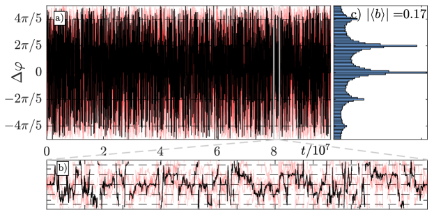
Figure 1: Time evolution of the Haus master equation with larger noise of the amplitude $\sigma=10^{-3}$ compared to figure 3 of the main text where $\sigma=4\times 10-4$.

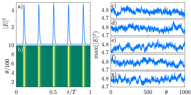
Figure 2: Short extract of the time trace from Fig. 1. a) Profile at the last step of the simulation. b) Evolution of $\left|E\right|^{2}$ over $10^{3}$ roundtrips. c)-g) Evolution of the maxima of the five pulses in a),b).

IV Positions of the beat notes in the RF spectrum

For an HML_N state in one of the splay phase configurations the spacing between neighboring teeth in the spectrum is $N$ times the fundamental frequency $\nu_{FSR}=\frac{2\pi}{\tau}$: $\Delta\nu=N\nu_{FSR}$. Therefore, the spectrum consists of peaks located at $\nu_{k}=\nu_{0}+k\Delta\nu$, where $k\in\mathbb{Z}$ and $\nu_{0}$ is some offset around which the comb is centered. Further, in the RF spectrum the main peaks are also separated by $\Delta\nu$ and the CW beam has a frequency $\nu_{CW}$. Hence, the beat notes in the RF spectrum for a given comb are found at $\Delta\nu_{k}=\left|\nu_{CW}-\nu_{k}\right|$. In particular, the two beat notes with the lowest frequency (cf. the sketch in the main text) are found for the value of $m$ such that $\nu_{m}<\nu_{CW}<\nu_{m+1}$ and hence, $\Delta\nu_{m}=\nu_{CW}-\nu_{0}-m\Delta\nu$ and $\Delta\nu_{m+1}=\nu_{0}-\nu_{CW}+\left(m+1\right)\Delta\nu$. For simplicity, we define $\Delta\nu_{0}=\Delta\nu_{m}+m\Delta\nu=\nu_{CW}-\nu_{0}$. Combining these results, we obtain

$$\Delta\nu_{k}=\begin{cases}+\Delta\nu_{0}-k\Delta\nu&k\leq m\\ -\Delta\nu_{0}+k\Delta\nu&k>m\end{cases}.$$ (35)

This explains why in each interval of length $\Delta\nu$ in the RF spectrum two beat notes are found corresponding to the interaction with the teeth of the comb located to the left (index $m$) and to the right (index $m+1$) of the CW frequency. For a visualization of the notation introduced above see Fig. 3.

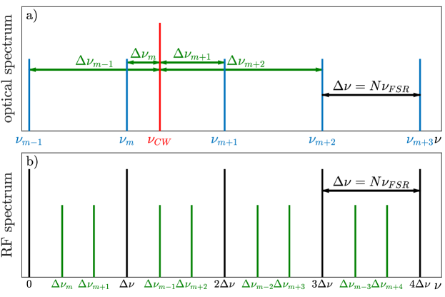
Figure 3: a) The optical spectrum of HML_N state in a splay phase configuration where the peaks of the comb are separated by $N\nu_{FSR}$. We use a CW beam (red) to create beat notes (green). b) The RF spectrum with the beat notes shown in a).

IV.1 Going from one frequency comb to the next one

In the main text, we explained that each HML_N solution has $N$ steady states corresponding to the phase differences $\Delta\varphi_{p}=\frac{2\pi p}{N}$ where $p=1,\dots,N$ which correspond to a shift of the frequency comb by $p\nu_{FSR}=p\frac{2\pi}{\tau}$. Hence, $\nu_{0}$ is shifted by $p\nu_{FSR}$. Therefore, we introduce the index $p$ in the previous notation such that $\Delta\nu_{k}^{\left(p\right)}=\left|\nu_{CW}-\nu_{k}^{(p)}\right|$ where $\nu_{k}^{(p)}=\nu_{0}-p\nu_{FSR}+k\Delta\nu$. Hence, in general, there are $2N$ possible positions for the beat notes in each interval of size $\Delta\nu$ in the RF spectrum (cf. Fig. 4).

Next, we want to make conclusions on the phase relation of the pulses in two different RF spectra $p$ and $q$ based on the respective locations of the beat notes. We consider the beat notes $\Delta\nu_{m,+}^{\left(p\right)}$ and $\Delta\nu_{m,+}^{\left(q\right)}$. As expected, the distance between these quantities gives a multiple of $\Delta\nu$

$$\Delta\nu_{m}^{\left(p\right)}-\Delta\nu_{m}^{\left(q\right)} =\Delta\nu_{0}^{\left(p\right)}-m\Delta\nu-\Delta\nu_{0}^{\left(q\right)}+m\Delta\nu$$

$$=\left(p-q\right)\nu_{FSR}$$ (36)

In the same way, we can also relate the left and the right beat notes of two different spectra $p$ and $q$

$$\Delta\nu_{m}^{\left(p\right)}+\Delta\nu_{m+1}^{\left(q\right)} =\Delta\nu_{0}^{\left(p\right)}-m\Delta\nu-\Delta\nu_{0}^{\left(q\right)}+(m+1)\Delta\nu$$

$$=\left(p-q\right)\nu_{FSR}+\Delta\nu.$$ (37)

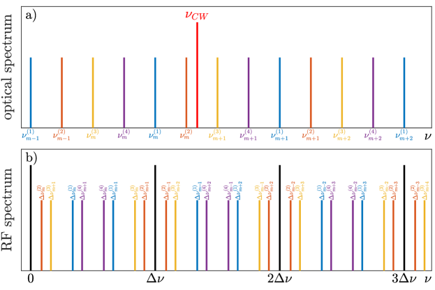
Figure 4: a) The optical spectrum of HML₄ state in a non-splay phase configuration. Here, the comb is a superposition of the four sub-combs shown in green, orange, yellow and purple. The separation of two e.g. blue peaks is $\Delta\nu=4\nu_{FSR}$ while neighboring peaks (e.g. blue and orange) are separated by $\nu_{FSR}$. We use a CW beam (red) to create beat notes. b) The RF spectrum with the beat notes. In each interval of size $\Delta\nu$, we find 8 beat notes.

V Experimental setup

The experimental setup is shown in Fig. 5. It consists in a Vertical External-Cavity Surface-Emitting Laser (VECSEL) delimited by an optically pumped InGaAs gain mirror emitting at 1060 nm and by a Semiconductor saturable Absorber Mirror (SESAM). The layout of the VECSEL cavity is similar to the one described in [1] and it is operated in the regime of temporal localized structures where multiple mode-locked pulses circulate in the resonator and each pulse can be individually addressed by shining short pump pulses inside the cavity [1]. For the heterodyne measurement, we use a tunable Littman-Metcalf diode laser system from Sacher with a linewidth smaller than 100 kHz. The resolution of the spectral detection is set by the RF power analyzer and amounts to 300 kHz.

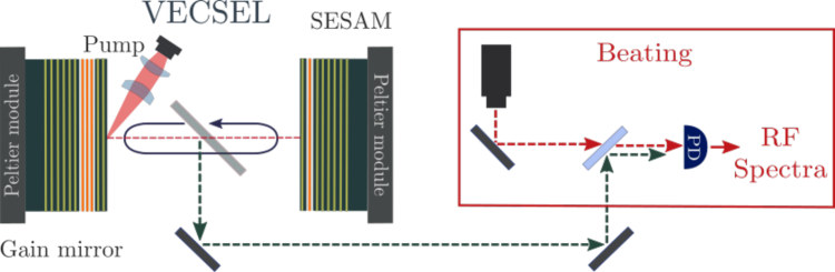
Figure 5: Experimental setup of the mode-locked VECSEL and detection. PEM: Piezo-Electric Mirror. PD: Photodiode. The heterodyne beating is realized between a tunable laser source (red arrow) and the VECSEL output (green arrow).

VI Experimental results with a splay state of 6 pulses

Lastly, Fig. 6 shows that coherent splayed state and incoherent pulse trains can be obtained for a larger number of pulses in the external cavity. Similarly to the 4 pulses case, Fig. 6 shows a splayed state of 6 pulses (panel a) and an incoherent phase state (panel b).

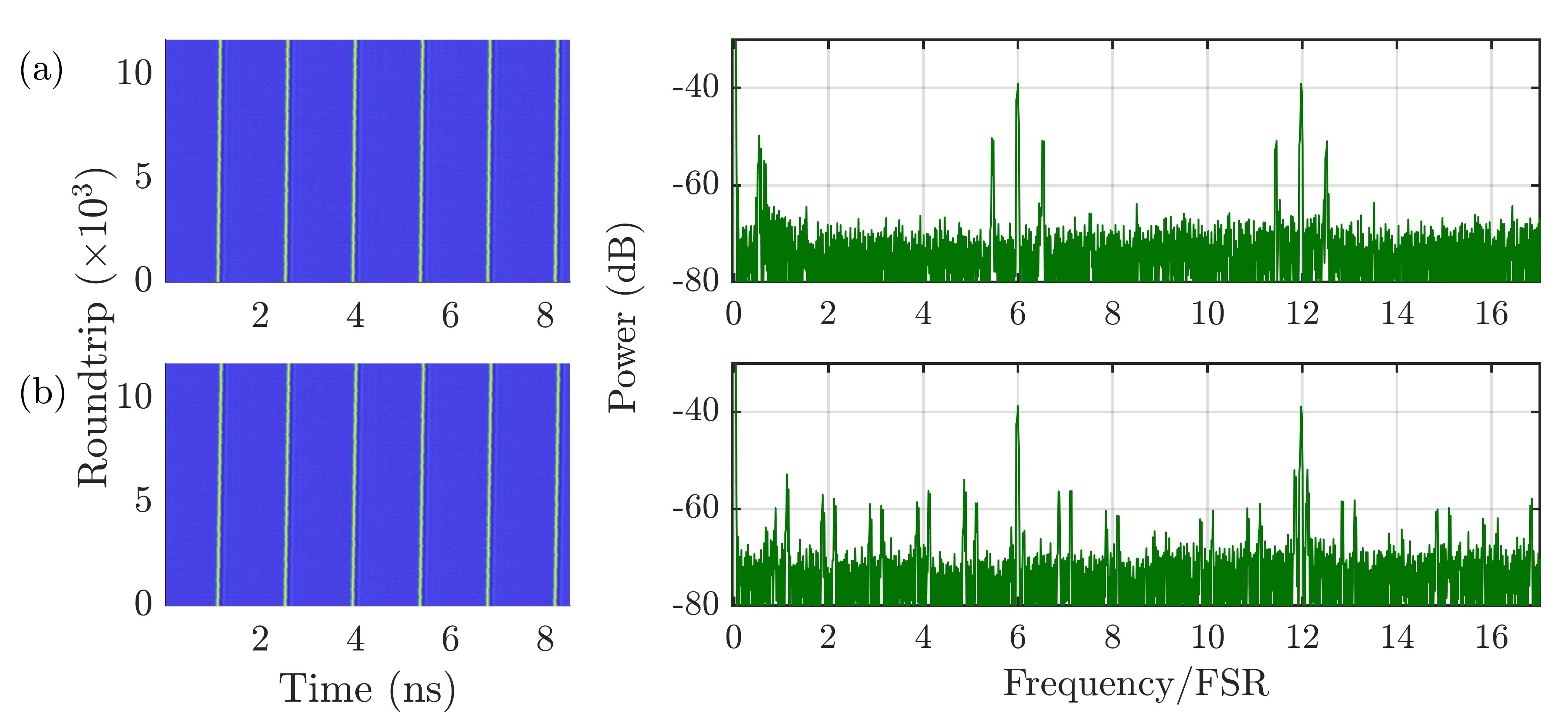
Figure 6: Analysis of the splayed states of 6 pulses emitted by the mode-locked VECSEL. Left column: spatio-temporal maps of the laser intensity. Right column: RF spectrum of the heterodyne beating signal. a) Coherent splayed states. b) Incoherent state characterized by the average spectral emission composed by spectral lines separated by 1 FSR.

VII References

[1] A. Bartolo, N. Vigne, M. Marconi, G. Beaudoin, K. Pantzas, I. Sagnes, G. Huyet, F. Maucher, SV Gurevich, J. Javaloyes, A. Garnache and M. Giudici, Temporal localized Turing patterns in mode-locked semiconductor lasers, Optica 9, 1386-1393 (2022).