Exergetic Port-Hamiltonian Systems
Modeling Language

Abstract

Mathematical modeling of real-world physical systems requires the consistent combination of a multitude of physical laws and phenomenological models. This challenging task can be greatly simplified by hierarchically decomposing systems. Moreover, the use of diagrams for expressing such decompositions helps make the process more intuitive and facilitates communication, even with non-experts. As an important requirement, models have to respect fundamental physical laws such as the first and the second law of thermodynamics. While some existing modeling frameworks can make such guarantees based on structural properties of their models, they lack a formal graphical syntax. We present a compositional and thermodynamically consistent modeling language with a graphical syntax. As its semantics, port-Hamiltonian systems are endowed with further structural properties and a fixed physical interpretation such that thermodynamic consistency is ensured in a way that is closely related to the GENERIC framework. While port-Hamiltonian systems are inspired by graphical modeling with bond graphs, neither the link between the two, nor bond graphs themselves, can be easily formalized. In contrast, our syntax is based on a refinement of the well-studied operad of undirected wiring diagrams. The language effectively decouples the construction of complex models via the graphical syntax from physical concerns, which are dealt with only at the level of primitive subsystems that represent elementary physical behaviors. As a consequence, reuse of models and substitution of their parts becomes possible. Finally, by construction, systems interact by exchanging exergy, i.e. energy that is available for doing work, so the language is particularly well suited for thermodynamic analysis and optimization.

1 Introduction

In this introduction we want to answer the following questions:

1. What are Exergetic Port-Hamiltonian Systems (EPHS)?

2. How do they enable compositional modeling?

3. Why is this practically relevant?

In addition, we briefly summarize key ideas of nonequilibrium thermodynamics and we discuss related work that inspired our developments. The introduction finishes with an outline of the main part of the paper.

1.1 What?

EPHS provide a compositional and thermodynamically consistent language for expressing mathematical models of multiphysical systems at macroscopic scales. Such systems may combine

1. classical mechanics
   (e.g. spring-mass systems, multibody dynamics, fluid mechanics),

2. classical electromagnetism
   (e.g. LC circuits, electromagnetic wave propagation)

3. and irreversible processes with local thermodynamic equilibrium
   (e.g. friction/viscosity, electrical resistance/conduction, thermal conduction).

The EPHS language is termed compositional since it enables a completely modular and hierarchical specification of models based on its simple graphical syntax, which is discussed in more detail in the next subsection.

If one flattens any hierarchical nesting of systems, one finds that every system is determined by a power-preserving interconnection of primitive subsystems. There are three main classes of primitive systems:

1. Systems that represent energy storage are characterized by a function which yields the stored energy for each possible state of the primitive system.

2. Systems that represent reversible energy exchange are characterized by a so-called Dirac structure, as known e.g. from (constrained) mechanical systems [1].

3. Systems that represent irreversible energy exchange are characterized by another type of structure that we call Onsager structure.

Since both classical mechanics and electromagnetism can be expressed using Dirac structures, item 2. corresponds to (a) and (b) above, while item 3. corresponds to (c). Structural properties of the primitive systems guarantee that all models respect the first and the second law of thermodynamics, Onsager’s reciprocal relations, as well as further conservation laws (e.g. for mass). Section 1.4 aims for a very brief introduction to nonequilibrium thermodynamics.

1.2 How?

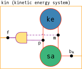
Figure 1: Graphical representation of an interconnection pattern with different syntactic elements shown in a different color. The outer box shown in orange represents the interface of the resulting composite system. The two protruding lines correspond to its ports called $\mathtt{f}$ and $\mathtt{b_{k}}$. The two inner boxes shown in red represent (the interface of) the subsystems called $\mathtt{ke}$ (storage of kinetic energy) and $\mathtt{sa}$ (self-advection of kinetic energy). Both have ports called $\mathtt{p}$ (momentum) and $\mathtt{m}$ (mass), while $\mathtt{sa}$ has another port called $\mathtt{b_{k}}$ (advection of kinetic energy across the boundary of the spatial domain). The port combinator shown in purple combines the ports $\mathtt{p}$ (fluid momentum) and $\mathtt{m}$ (fluid mass) into the multiport $\mathtt{f}$ (fluid). The black dots represent junctions where power is exchanged among the connected ports. The dashed line indicates that port $\mathtt{m}$ of the port combinator does not partake in power exchange, but merely shares information about the state (fluid mass).

Expressions in the graphical syntax are called interconnection patterns because a pattern specifies how a composite system can be formed through a power-preserving interconnection of subsystems. Figure 1 shows an example from fluid dynamics.

The syntax deals with systems only in terms of their interfaces, i.e. their exposed ports. Each port has two attributes: The first attribute gives the physical quantity that can be exchanged via the port together with the corresponding state space. To rule out ill-defined connections, only ports with the same quantity can be connected. The second attribute is of Boolean type and indicates whether power can be exchanged over the port or merely information about system state, as indicated graphically by a solid or a dashed line, respectively.

An interconnection pattern should be thought of as a function which, for every round inner box, takes as input a system with matching interface and returns a system whose interface matches the outer box. For instance, the pattern shown in Figure 1 represents a function which takes two subsystems whose interfaces are determined by the ports of the boxes $\mathtt{ke}$ and $\mathtt{sa}$, and it returns a composite system whose interface is determined by the ports of the outer box. In the graphical representation, we often draw inner boxes filled with a color that indicates the nature of the subsystems that we consider as inputs. In Figure 1, $\mathtt{ke}$ has a blue filling as it represents energy storage, i.e. the fluid’s kinetic energy, while $\mathtt{sa}$ has a green filling as it represents reversible energy exchange, i.e. the advection of momentum and mass by the fluid flow. Written on top of the outer box, kin is an identifier akin to a function name and the text in parenthesis is just a short description. The port combinator and the corresponding multiport $\mathtt{f}$ are syntactic sugar that allows the composite system to be connected to other systems without drawing parallel connections.

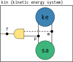
(a) Kinetic energy system

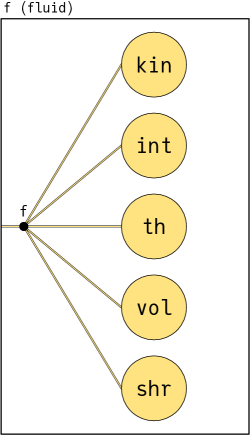
(b) Fluid system

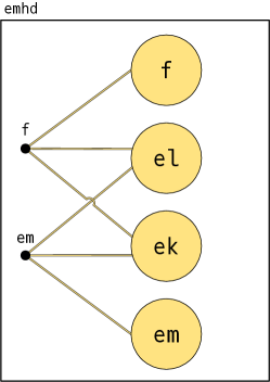
(c) EMHD System

Figure 2: Hierarchical specification of an electro-magneto-hydrodynamics model: The fluid model f shown in (b) comprises the kinetic energy system kin shown in (a) and four further models which are not shown, namely an internal energy system int, a thermal conduction model th, and volume / shear viscosity models vol / shr. The electro-magneto-hydrodynamics model emhd shown in (c) comprises the fluid model f and three further models which are not shown, namely an electro-magnetic system em, an electric conduction model el, and a model for the electro-kinetic coupling ek.

Figure 2 demonstrates the hierarchical specification of a model for electro-magneto-hydrodynamics. For simplicity, a spatial domain with empty or isolated boundary is assumed such that only the in-domain interconnection of the different models needs to be dealt with. The yellow filling of the inner boxes in Figures 2(b) and 2(c) indicates that another composite system, which in turn is specified with its own interconnection pattern, is supplied as input. Recursively substituting into all yellow inner boxes the respective interconnection patterns would yield an equivalent model specification without hierarchical decomposition. The composition of interconnection patterns through substitution is uniquely defined as long as interfaces match. Similarly, one can add a level of nesting by refactoring a number of subsystems into a reusable composite subsystem. In the fluid model, one could for instance factor out the kinetic energy system filling the box $\mathtt{kin}$ and the internal energy subsystem filling the box $\mathtt{int}$ into a reusable ideal compressible fluid model.

1.3 Why?

EPHS provide a formal and intuitive modeling language suited for humans and software tools alike. As shown above, increasingly complex models can be assembled from simpler and ultimately primitive parts. This fosters the reusability of models and encourages the conceptual separation of different levels of detail. Beyond the modeling process, this provides value in interdisciplinary communication and education. Some modeling errors can be completely avoided due to typed interfaces (given by ports with fixed physical quantities) and the built-in thermodynamic consistency. Since interconnection patterns can be used as exergy flow diagrams, EPHS models are particularly useful for thermodynamic analysis and optimization. The compositional nature of EPHS could enable a scalable approach to model transformations, such as discretizations, and also to the integration of scientific machine learning techniques in first-principles-based physical modeling.

1.4 Nonequilibrium thermodynamics in a tiny nutshell

Most physical systems are characterized by a huge number of degrees of freedom but keeping track of them is usually neither possible nor useful. Nonequilibrium thermodynamics aims to provide a framework for coarse-grained modeling, meaning that fast dynamics at small scales are not resolved and a quantity called entropy is introduced to account for the missing information, see e.g. [2]. Coarse-graining is possible because, despite of fluctuations at the microscopic scale, one can eventually observe non-fluctuating properties at a more macroscopic scale; at least this is the case for isolated systems. For instance, temperature is a property that does not appear at the microscopic scale. Thermodynamic properties are classified as extensive when they are proportional to the size of the system (e.g. entropy, volume, mass) or as intensive when they do not depend on the size of the system (e.g. temperature, pressure, chemical potential), see e.g. [3]

A system is said to be in local thermodynamic equilibrium if for every material point there exists a neighborhood large enough to observe thermodynamic properties, yet small enough for the properties to be non-varying inside the neighborhood, see e.g. [4]. The size of these neighborhoods presents a macroscopic scale at which the dynamics of the thermodynamic properties can be observed and also modeled.

The first law of thermodynamics just restates a well-known fact from mechanics, namely that energy is a conserved quantity. However, instead of considering directly the mechanical and electromagnetic energy associated to microscopic degrees of freedom, a thermodynamic model with local equilibrium resorts to a phenomenological description called internal energy, which is considered to depend on a number of extensive properties, including entropy, and possibly further mechanical or electromagnetic state variables which are observable on the considered macroscopic scale. These quantities then serve as the state variables of a coarse-grained description. Moreover, temperature is the derivative of the internal energy with respect to entropy. Similarly, pressure is given by the derivative with respect to volume and the chemical potential is the derivative with respect to mass, see e.g. [3].

Classical mechanics and electromagnetism exhibit reversible dynamics, meaning that one could in principle arrive again at the initial condition by reversing the direction of time (although for many systems this would be impossible due to chaos). Incomplete knowledge about the microscopic state immediately leads to irreversible dynamics and an irreversible dynamics in turn leads to a growth of entropy, as information (e.g. about the initial state of the system) is lost in the process. This is reflected by the second law of thermodynamics which states that the entropy of an isolated system never decreases and that the system evolves towards a state of maximum entropy, see e.g. [4]. In other words, the uncertainty about the microscopic state can only grow, not decrease.

For models with local equilibrium, the irreversible dynamics can be expressed in terms of so-called thermodynamic fluxes that determine instantaneous changes of coarse-grained state variables. The fluxes are expressed as a function of thermodynamic forces, which are given by differences in intensive quantities, see e.g. [4, 5]. For instance, temperature differences cause heat flux, according to Fourier’s law, and differences in chemical potential cause a diffusive mass flux, according to Fick’s law. Further, one may observe cross effects such as a diffusive mass flux caused by temperature differences (Soret effect) and likewise a heat flux caused by differences in chemical potential (Dufour effect). Onsager’s reciprocal relations state that the relation between fluxes and forces must possess a certain symmetry [6]. For instance, the ratio of the mass flux caused by the Soret effect and the respective temperature difference is equal to the ratio of the heat flux caused by the Dufour effect and the respective difference in chemical potential.

1.5 Related work

Figure 3 gives a high-level view of this subsection.

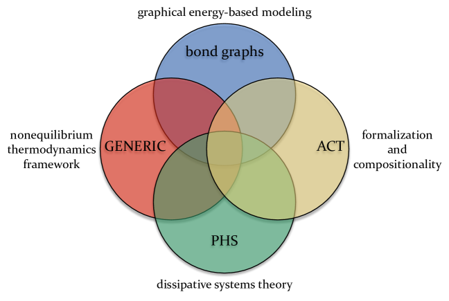
Figure 3: Informal Venn diagram illustrating that EPHS integrates ideas from graphical and energy-based modeling of physical systems with bond graphs, the GENERIC framework for nonequilibrium thermodynamics, the port-Hamiltonian theory of open dissipative systems (PHS), and applied category theory (ACT) research on the formalization of graphical languages and compositional dynamical systems.

1.5.1 Port-Hamiltonian systems

Apparent from their name, EPHS have a lot in common with Port-Hamiltonian Systems (PHS). PHS were originally inspired by relating the dynamical systems defined by generalized bond graphs [7] (i.e. bond graphs using a single kind of energy storage elements together with gyrator elements) to Hamiltonian mechanics [8]. While many authors make use of explicit input-output port-Hamiltonian systems, PHS constitute an acausal systems theory, inspired also by the behavioral approach of Willems [9, 10]. The dynamics of networks comprising energy storing elements and reversible coupling elements between them (such as generalized transformers and gyrators) can be formalized, from a geometric viewpoint, as a Hamiltonian system whose Poisson structure reflects the network topology [11]. The generalization to networks with algebraic constraints and externally controlled ports is achieved by using Dirac structures, which unify Poisson structures and presymplectic structures [12]. By specifying a resistive relation on external port variables, the implicit Hamiltonian dynamics can be combined with a dissipative gradient dynamics, allowing for network elements that represent e.g. dampers and resistors. The key properties of PHS are firstly a power-balance equation which states that the sum of the stored power and the dissipated power is equal to the supplied power (passivity) and secondly the possibility to combine port-Hamiltonian systems by composition of their Dirac structures with an interconnecting Dirac structure, see for instance [13].

While the dynamical systems defined by EPHS models are essentially PHS, they have further structural properties and a fixed physical interpretation. PHS in general have no uniform thermodynamic interpretation and they lack a formal graphical syntax to express their interconnection. In contrast to EPHS, PHS also lack a built-in mechanism for referring to subsystems and ports.

1.5.2 GENERIC framework

The general equation for reversible-irreversible coupling (GENERIC) provides a framework for combining reversible and irreversible dynamics in a way that respects fundamental thermodynamic principles, namely the first law, the second law and the reciprocal relations discovered by Onsager [14]. The reversible part is defined by an entropy-conserving Hamiltonian dynamics, while the irreversible part is given by an energy-conserving gradient flow, see e.g. [4]. We note that the same holds for closely-related earlier developments in this direction, including metriplectic systems, see [15, 16, 17, 18]. While a large class of well-known dynamical systems from physics can be identified as instances of the GENERIC, see e.g. [2], the framework is especially helpful for the development of new thermodynamic models.

The combination of Hamiltonian and gradient dynamics in both PHS and GENERIC systems led to the initial observation of a relationship between the two frameworks in [19]. GENERIC systems with local thermodynamic equilibrium can be seen as port-Hamiltonian systems, where the storage function corresponds to the system’s exergy. This function yields the maximum amount of work that can be extracted by an ideal (i.e. purely reversible) process which may arbitrarily interact with the system’s storage components and a given reference environment [20].

The dynamical systems defined by (isolated) EPHS models are basically GENERIC systems, since their built-in thermodynamic consistency and associated physical interpretation follow from the same ideas. Beyond the aspect of compositionality, there are two main differences: 1. GENERIC systems are more general in the sense of including systems beyond local thermodynamics equilibrium (where the concept of temperature does not apply). 2. The reversible part of EPHS is defined using Dirac structures, rather than less general Poisson structures (which cannot express kinematic constraints). This is crucial e.g. for modeling multibody systems and electrical circuits.

1.5.3 Bond graph modeling

Bond graph modeling is based on a graphical notation for representing dynamical systems and in particular multi-domain models involving mechanical and electrical elements [21, 22]. The main idea is that elements interact via bonds that represent links for energy exchange. Associated to each bond, there are two dynamic variables called flow and effort, whose product (or duality pairing) gives the exchanged power. Bonds can be connected via two types of junctions, namely $0$-junctions, where the flow variables of all connected ports balance, with all effort variables being equal, and dually defined $1$-junctions, where the effort variables balance, with all flow variables being equal. In both cases, the net power at a junction is zero.

While PHS can be seen as a geometric formalization of the dynamical systems defined by generalized bond graphs, the algebraic formalization of the bond graph notation itself is not straightforward, when compared to e.g. standard multigraphs, see [23, 24]. The inherent complexity of the notation is evident also in practice, since the direction in which exchange of power is counted positive and sometimes also the question which variable is flow and which is effort have to be decided arbitrarily, bond by bond. While bond graphs are frequently used in the literature to illustrate PHS, their use as a formal syntax for model specification is not established. Previous work has focused on algorithms for converting certain classes of bond graphs to port-Hamiltonian systems, see e.g. [25].

In contrast to bond graph notation, the EPHS syntax only has $0$-junctions and every interconnection pattern has an outer box. As demonstrated by various applications, a single type of junctions is sufficient and moreover the simplification entails crucial advantages: Interconnection patterns are easier to interpret, in particular due to the direct correspondence between junctions and energy domains. This correspondence arises from the inherent distinction between the roles of flows and efforts, a feature that is lacking in bond graphs. Further, the direction in which exchange of power is counted positive is predetermined in accordance with the convention used in thermodynamics, i.e. energy supplied to a system has a positive sign. Last but not least, interconnection patterns can be hierarchically composed and decomposed in a natural way.

1.5.4 Applied category theory

The compositional nature of EPHS can be made precise using category theory. Category theory was first applied in algebraic geometry and topology and now is used to organize many branches of mathematics [26]. In recent decades, category theory has also grown beyond pure math to organize scientific and engineering disciplines as well, giving birth to ‘applied category theory’ [27]. A specific approach to categorical systems theory [28] that has inspired this work is based on the following principles, which can essentially also be found in the work of Willems [10].

1. A shift of focus from individual systems to how systems relate to each other.

2. An isolated system is a system with empty interface.

3. The description of systems involves syntax and semantics. Syntax typically consists of combinatorial data that can be manipulated computationally, while semantics are given by geometric objects that exist only platonically. Additionally, the syntax can be displayed and manipulated diagrammatically as well as in text. An explicit understanding of the translation from syntax to semantics serves as a guide for computer implementation.

For instance, there is a line of research which formalizes graphical languages for systems and process such as block diagrams [29], Petri nets [30], junctions of bond graphs [24], and passive linear circuits [31]. These works consider a graphical syntax as some sort of string diagrams, established via a generators and relations approach.

More closely related to our work, another line of research uses the theory of operads to define a graphical syntax which supports hierarchical (de-)composition, see [32, 33]. Operads organize formal operations with finitely many inputs (subsystems) and one output (composite system), see [34, 35]. As proposed in [36], the EPHS syntax, is based on the operad of undirected wiring diagrams, which initially appeared in [37], together with its relational semantics used to express database queries, see also [38, 39, 40]. In a similar lane, directed wiring diagrams are used to formalize nested systems of Moore machines and ODEs with outputs, see [41, 42]. A combination of dynamical systems based on directed and undirected wiring diagrams is presented in [43, 44]. The composition of lossless port-Hamiltonian systems was recently studied from a categorical perspective in [45].

1.6 Outline

Section 2 defines system interfaces. Based on this, Section 3 defines interconnection patterns. Section 4 shows how every interconnection pattern implies a relation between the port variables of its interfaces. Section 5 discusses how exergy quantifies the energy stored in a system that is available for doing work. Based on this, Section 6 introduces the primitive systems. Section 7 defines composite systems and how they are formed using the graphical syntax. Section 8 shows that EPHS models are thermodynamically consistent. Section 9 presents an example of a motor model, together with a comparison to a classical bond graph. Section 10 concludes with a discussion.

2 Interfaces

While the narrative of discovery, usually proceeds from systems to interfaces, logically speaking, the syntax needs to be introduced before the semantics and hence we start with interfaces. Graphically, the interface of a system is a box with a set of ports drawn around it. While we could treat such sets abstractly, as is often done in applied category theory, for practical reasons we instead treat them as sets of names called namespaces.

2.1 Namespaces

Definition 2.1.

A string is a non-empty list of characters and a name is a list of strings. ∎

We write names using a monospace font and with strings separated by dots. For instance, the name consisting of the list of strings “oscillator”, “spring”, “q” is written as $\mathtt{oscillator.spring.q}$. Further, we use $[]$ to denote the empty name, i.e. the empty list of strings. Given two names $n$ and $n^{\prime}$, we denote their concatenation by $n\ast n^{\prime}$. For example, $\mathtt{a.b}\ast\mathtt{c}=\mathtt{a.b.c}$.

Definition 2.2.

Given two names $p$ and $n$, we say that $p$ is a prefix of $n$, and write $p\leq n$ if there exists any name $s$ such that $n=p\ast s$. In case $s\neq[]$, we say that $p$ is a strict prefix of $n$ and write $p<n$. ∎

Example 2.3.

It holds that $\mathtt{a.b}<\mathtt{a.b.c}$ and $\mathtt{a.b}\leq\mathtt{a.b}$. Also $[]<\mathtt{a}$. It does not hold that $\mathtt{a.a}\leq\mathtt{a}$. ∎

Definition 2.4.

A set of names $N$ is prefix-free if for all $n,n^{\prime}\in N$, $n$ is not a strict prefix of $n^{\prime}$. A namespace is a finite, prefix-free set of names. Let $\mathbf{Namespace}$ refer to the set of all namespaces. ∎

Example 2.5.

The set of names $\{\mathtt{a},\,\mathtt{b}\}$ is a namespace and so is $\{\mathtt{a.a},\,\mathtt{a.b}\}$. Since $\mathtt{a}<\mathtt{a.b}$, the set of names $\{\mathtt{a},\,\mathtt{a.b}\}$ is not prefix-free and hence not a namespace. ∎

Sets of names are equivalent to prefix trees, called tries in computer science [46].

Example 2.6.

The namespace $\{\mathtt{a.b.b},\,\mathtt{a.b.c},\,\mathtt{b.a},\,\mathtt{b.y},\,\mathtt{c}\}$ corresponds to the following trie:

$$\includegraphics{figures/namespaces/namespace-tree}\qed$$

Note that for a namespace $N$, the leaf nodes of its trie correspond to the names in $N$, while for a set of names, which is not prefix-free, at least one name corresponds to an internal node. In the following, we think of namespaces both as sets of names and as tries.

Given several namespaces, we could take their union as sets. However, this runs the risk of name conflicts, as it is possible for a given name in the union to have come from either of the original sets. It is for this reason that we introduce the concept of a named sum, which can be thought of as a practical implementation of disjoint union.

Definition 2.7.

Given a namespace $N$, and a function $f\colon N\to\mathbf{Namespace}$, the named sum of $f$ is

$$\sum f\>=\>\Bigl{\{}n\ast a\,\mid\,n\in N,\>a\in f(n)\Bigr{\}}\,.\qed$$

We also sometimes write expressions like $\sum\left[\mathtt{a}\mapsto I_{1},\,\mathtt{b}\mapsto I_{2}\right]$, which refers to the named sum of the anonymous function defined by

$$x\>\mapsto\>\begin{cases}I_{1}&\text{if }x=\mathtt{a}\\ I_{2}&\text{if }x=\mathtt{b}\,.\end{cases}$$

Example 2.8.

Given $N=\{\mathtt{q},\,\mathtt{p.1},\,\mathtt{p.2}\}$, we have

$$\sum\left[\mathtt{l}\mapsto N,\,\mathtt{s.t}\mapsto N\right]\>=\>\bigl{\{}\mathtt{l.q},\,\mathtt{l.p.1},\,\mathtt{l.p.2},\,\mathtt{s.t.q},\,\mathtt{s.t.p.1},\,\mathtt{s.t.p.2}\bigr{\}}\,.\qed$$

Proposition 2.9.

Given a namespace $N$ and a function $f\colon N\to\mathbf{Namespace}$, the named sum $\sum f$ is again a namespace, that is to say it is prefix-free. ∎

Proof.

The trie $\sum f$ is simply the trie $N$ with, for each leaf node $n\in N$, the trie $f(n)$ grafted on top. ∎

Namespaces and named sums provide a simple and effective formalism for working with large hierarchically-structured systems.

2.2 Packages

An interface has a namespace, where we interpret each name as referring to a port. However, this is not the only ingredient to an interface, as each port has two associated attributes. This motivates the definition of packages:

Definition 2.10.

Given a set $A$, we define

$$\mathbf{Pkg}(A)\>=\>\Bigl{\{}(N,\,\tau)\,\mid\,N\in\mathbf{Namespace},\,\tau\colon N\to A\Bigr{\}}\,.$$

An element $(N,\,\tau)\in\mathbf{Pkg}(A)$ is called a package of elements of $A$. We also just write $\tau\in\mathbf{Pkg}(A)$ with $N=\operatorname{dom}(\tau)$. ∎

The name ‘package’ is drawn from software engineering; one might consider a software package to be a ‘package of types and procedures’.

A package $(N,\,\tau)\in\mathbf{Pkg}(A)$ can be seen as a trie $N$ with an element $\tau(n)\in A$ associated to each leaf node $n\in N$. Hence, the concept of named sum carries over from $\mathbf{Namespace}$ to $\mathbf{Pkg}(A)$, for a fixed set $A$. Named sum can then be seen as a flattening operation, analogous to flattening a list of lists. Specifically, for the set of all lists of elements of $A$

$$\operatorname{\mathbf{List}}(A)\>=\>\bigl{\{}(n,\,f)\,\mid\,n\in\mathbb{N},\,f\colon\{1,\,\ldots,\,n\}\to A\bigr{\}}\,,$$

flattening is a map $\operatorname{\mathbf{List}}(\operatorname{\mathbf{List}}(A))\to\operatorname{\mathbf{List}}(A)$, which for instance sends $[[1,\,2],\,[3,\,4]]$ to $[1,\,2,\,3,\,4]$. Similarly, named sum is a map $\mathbf{Pkg}(\mathbf{Pkg}(A))$ to $\mathbf{Pkg}(A)$. An input to this is a trie $N$, which has associated to each leaf node $n\in N$ another trie $N_{n}$, whose leaves carry elements of $A$. The named sum operation then simply grafts onto each node $n\in N$ its associated trie $N_{n}$, carrying along the elements of $A$ at the leaves. In terms of category theory, the flattening operation makes $\operatorname{\mathbf{List}}$ and $\mathbf{Pkg}$ examples of monads.

2.3 Bundle of quantities

The first attribute associated to any port represents the physical quantity that can be exchanged via the port, e.g. entropy or momentum, along with a state space in which values of the quantity live. For instance a momentum variable can take values in $\mathbb{R}$ if motion along a single axis is considered or it can take values in the vector space $\mathfrak{se}^{*}(3)$ if rigid body motions in $3$-dimensional Euclidian space are considered, etc.

Definition 2.11.

Let $\mathbf{S}$ be a finite set of state spaces (i.e. smooth manifolds) and for each space $\mathcal{X}\in\mathbf{S}$, let $\mathbf{Q}_{\mathcal{X}}$ be a finite set of physical quantities taking values in $\mathcal{X}$. Further, let $\mathbf{Q}$ be the disjoint union of all quantities, i.e.

$$\mathbf{Q}\>=\>\bigsqcup_{\mathcal{X}\in\mathbf{S}}\mathbf{Q}_{\mathcal{X}}\,.$$

This forms a bundle of quantities (in the category of finite sets), whose projection

$$\mathrm{space}:\mathbf{Q}\twoheadrightarrow\mathbf{S}$$

returns the underlying space of a quantity. ∎

Example 2.12.

The bundle of quantities given by

$$\begin{split}\mathbf{S}\>&=\>\{\mathbb{R},\,\mathrm{SE}(3),\,\mathfrak{se}^{*}(3)\}\\ \mathbf{Q}_{\mathbb{R}}\>&=\>\{\mathtt{displacement},\,\mathtt{momentum},\,\mathtt{entropy},\,\mathtt{volume}\}\\ \mathbf{Q}_{\mathrm{SE}(3)}\>&=\>\{\mathtt{pose}\}\\ \mathbf{Q}_{\mathfrak{se}^{*}(3)}\>&=\>\{\mathtt{momentum}\},\end{split}$$

would be sufficient for some spatially-lumped models from mechanics and thermodynamics. A port with associated quantity $q=(\mathbb{R},\,\mathtt{entropy})\in\mathbf{Q}$ can exchange entropy and its associated state space is $\mathrm{space}(q)=\mathbb{R}\in\mathbf{S}$. ∎

To distinguish reversible and irreversible dynamics later on in Sections 6.3 and 6.4, we make use of the concept of parity, see [47, 20] for details.

Definition 2.13.

Let the parity of each quantity with respect to time-reversal transformation be given by a function $\mathrm{P}:\mathbf{Q}\rightarrow\{-1,\,+1\}$. ∎

Example 2.14.

For the bundle of quantities from 2.12, we have

$$\mathrm{P}(\mathbb{R},\,\mathtt{displacement})=+1$$

$$\mathrm{P}(\mathbb{R},\,\mathtt{momentum})=-1$$

$$\mathrm{P}(\mathbb{R},\,\mathtt{entropy})=+1$$

$$\mathrm{P}(\mathbb{R},\,\mathtt{volume})=+1$$

because displacement, entropy, and volume do not change instantaneously when a recording is suddenly played backwards (positive parity), whereas momentum changes its sign (negative parity). ∎

A comprehensive collection of physical quantities with their associated parities would be a built-in feature of a software implementation.

2.4 Interfaces as packages

Each port has two attributes, namely the already discussed quantity and further a Boolean attribute that indicates whether the port is a power port or a state port. Only power ports allow for exchange of energy associated with the attributed quantity. A state port is required whenever the behavior of a system depends on the state of another system, although no energy is exchanged between the two.

Definition 2.15.

An interface is a package of elements of $\mathbf{Q}\times\{\mathsf{p},\mathsf{s}\}$, i.e. let

$$\mathbf{Interface}\>=\>\mathbf{Pkg}\bigl{(}\mathbf{Q}\times\{\mathsf{p},\mathsf{s}\}\bigr{)}\,.\qed$$

Example 2.16.

Let $I=(N,\,\tau)$ be an interface with namespace $N=\{\mathtt{p_{1}},\,\mathtt{p_{2}},\,\mathtt{q}\}$ and attributes given by $\tau(\mathtt{p_{1}})=\tau(\mathtt{p_{2}})=\left((\mathbb{R},\,\mathtt{momentum}),\,\mathsf{p}\right)$ and $\tau(\mathtt{q})=\left((\mathbb{R},\,\mathtt{displacement}),\,\mathsf{s}\right)$. Ports $\mathtt{p_{1}}$ and $\mathtt{p_{2}}$ are power ports that can exchange kinetic energy, along with information about the current momentum. Port $\mathtt{q}$ is a state port that can only exchange information about the current displacement. ∎

We note that the named sum of interfaces is a function $\mathbf{Pkg}(\mathbf{Interface})\to\mathbf{Interface}$.

2.5 Bundles of port variables

A state port has one port variable called state. A power port has two further port variables called flow and effort. Given an interface, the port variables of all its ports combined together take values in a vector bundle, called the bundle of port variables associated to the interface.

Definition 2.17.

Let $I=(N,\,\tau)$ be an interface and let $p\in I$ be a port, i.e. $p\in N$.
The state space associated to port $p$ is

$$\mathcal{X}_{p}\>=\>(\mathrm{space}\circ\mathrm{pr}_{1}\circ\tau)(p)\,,$$

where $\mathrm{pr}_{1}$ projects onto the first attribute, i.e. the quantity.
The state space associated to interface $I$ is the Cartesian product

$$\mathcal{X}_{I}\>=\>\prod_{p\,\in\,I}\mathcal{X}_{p}\,.\qed$$

Example 2.18.

Let $I_{\text{gas}}=(N_{\text{gas}},\,\tau_{\text{gas}})$ be an interface with namespace $N_{\text{gas}}=\{\mathtt{s},\,\mathtt{v}\}$ and attributes given by $\tau_{\text{gas}}(\mathtt{s})=\left((\mathbb{R},\,\mathtt{entropy}),\,\mathsf{p}\right)$, $\tau_{\text{gas}}(\mathtt{v})=\left((\mathbb{R},\,\mathtt{volume}),\,\mathsf{p}\right)$. Then, its associated state space is $\mathcal{X}_{I_{\text{gas}}}=\mathcal{X}_{\mathtt{s}}\times\mathcal{X}_{\mathtt{v}}=\mathbb{R}\times\mathbb{R}$. Let $I_{\text{mass}}=(N_{\text{mass}},\,\tau_{\text{mass}})$ be another interface with $N_{\text{mass}}=\{\mathtt{p}\}$ and $\tau_{\text{mass}}(\mathtt{p})=\left((\mathbb{R},\,\mathtt{momentum}),\,\mathsf{p}\right)$. Then, the named sum

$$I\>=\>(N,\,\tau)\>=\>\sum[\mathtt{gas}\mapsto I_{\text{gas}},\,\mathtt{mass}\mapsto I_{\text{mass}}]$$

has the namespace $N=\{\mathtt{gas.s},\,\mathtt{gas.v},\,\mathtt{mass.p}\}$ with attributes given by $\tau(\mathtt{gas.s})=\left((\mathbb{R},\,\mathtt{entropy}),\,\mathsf{p}\right)$, $\tau(\mathtt{gas.v})=\left((\mathbb{R},\,\mathtt{volume}),\,\mathsf{p}\right)$, $\tau(\mathtt{mass.p}))=\left((\mathbb{R},\,\mathtt{momentum}),\,\mathsf{p}\right)$. We note that

$$\mathcal{X}_{I}\>=\>\mathcal{X}_{I_{\text{gas}}}\times\mathcal{X}_{I_{\text{mass}}}\,.\qed$$

Given any interface $I$, each port $p\in I$ has an associated state variable $p\mathtt{.x}\in\mathcal{X}_{p}$. If $p$ is a power port, it additionally has a flow variable $p\mathtt{.f}$ and an effort variable $p\mathtt{.e}$. All port variables implicitly depend on time. As detailed in Section 6.1, the flow variable is the instantaneous rate of change of the state variable and the effort variable is the differential of a function of the state variable. Hence, we have $\left(p\mathtt{.x},\,p\mathtt{.f},\,p\mathtt{.e}\right)\in\mathbb{T}\mathcal{X}_{p}$, where $\mathbb{T}\mathcal{X}_{p}=\mathrm{T}\mathcal{X}_{p}\oplus\mathrm{T}^{*}\mathcal{X}_{p}$ denotes the direct sum (or Whitney sum) of the respective tangent and cotangent bundles (see e.g. [48]). The flow and effort variables are called power variables because their duality pairing $\langle p\mathtt{.e}\mid p\mathtt{.f}\rangle\in\mathbb{R}$ yields the instantaneous power that is exchanged through port $p$.

Now we can define the bundle of port variables associated to an interface:

Definition 2.19.

Let $I$ be an interface. Based on the Boolean attribute of its ports, we can write its associated state space as the Cartesian product $\mathcal{X}_{I}\cong\mathcal{X}_{I,p}\times\mathcal{X}_{I,s}$, where $\mathcal{X}_{I,p}$ is the state space of all power ports and $\mathcal{X}_{I,s}$ is the state space of all state ports. Accordingly, we let $x=(x_{p},\,x_{s})\in\mathcal{X}_{I,p}\times\mathcal{X}_{I,s}$ denote all state variables and we let $(f,\,e)\in\mathbb{T}_{x_{p}}\mathcal{X}_{I,p}$ denote all flow and effort variables. The bundle of port variables $\mathrm{pr}_{I}:\mathcal{P}_{I}\twoheadrightarrow\mathcal{X}_{I}$ associated to interface $I$ is defined as the pullback bundle of $\mathbb{T}\mathcal{X}_{I,p}$ along the projection $\mathrm{pr}_{p}:\mathcal{X}_{I,p}\times\mathcal{X}_{I,s}\twoheadrightarrow\mathcal{X}_{I,p}$. Hence, $\mathcal{P}_{I}\cong\mathbb{T}\mathcal{X}_{I,p}\times\mathcal{X}_{I,s}$.

$$\leavevmode\hbox to250.9pt{\vbox to104.74pt{\text{[drawing]}}}\qed \mathbb{T}\mathcal{X}_{I,p} \color[rgb]{.5,.5,.5}\ni(x_{p},\,f,\,e) \color[rgb]{.5,0,.5}\mathcal{P}_{I} \color[rgb]{.5,.5,.5}\ni(x,\,f,\,e) \mathcal{X}_{I,p} \color[rgb]{.5,.5,.5}\ni x_{p} \mathcal{X}_{I} \color[rgb]{.5,.5,.5}\ni x \mathcal{X}_{I,s} \color[rgb]{.5,.5,.5}\ni x_{s} \scriptstyle{\mathrm{pr}_{p}} \scriptstyle{\mathrm{pr}_{s}} \scriptstyle{\definecolor[named]{.}{rgb}{.5,0,.5}\color[rgb]{.5,0,.5}\mathrm{pr}_{\mathtt{I}}} \scriptstyle{\definecolor[named]{.}{rgb}{.5,0,.5}\color[rgb]{.5,0,.5}\lrcorner} \mathbb{T}\mathcal{X}_{I,p} \color[rgb]{.5,.5,.5}\ni(x_{p},\,f,\,e) \color[rgb]{.5,0,.5}\mathcal{P}_{I} \color[rgb]{.5,.5,.5}\ni(x,\,f,\,e) \mathcal{X}_{I,p} \color[rgb]{.5,.5,.5}\ni x_{p} \mathcal{X}_{I} \color[rgb]{.5,.5,.5}\ni x \mathcal{X}_{I,s} \color[rgb]{.5,.5,.5}\ni x_{s} \scriptstyle{\mathrm{pr}_{p}} \scriptstyle{\mathrm{pr}_{s}} \scriptstyle{\definecolor[named]{.}{rgb}{.5,0,.5}\color[rgb]{.5,0,.5}\mathrm{pr}_{\mathtt{I}}} \scriptstyle{\definecolor[named]{.}{rgb}{.5,0,.5}\color[rgb]{.5,0,.5}\lrcorner}$$

Example 2.20.

Consider again the interface from 2.16. Its bundle of port variables $\mathcal{P}_{I}\twoheadrightarrow\mathcal{X}_{I}$ has total space (or port space)

$$\mathcal{P}_{I}\>=\>\mathbb{T}\mathbb{R}\times\mathbb{T}\mathbb{R}\times\mathbb{R}\>\ni\>\bigl{(}(\mathtt{p_{1}.x},\,\mathtt{p_{1}.f},\,\mathtt{p_{1}.e}),\,(\mathtt{p_{2}.x},\,\mathtt{p_{2}.f},\,\mathtt{p_{2}.e}),\,\mathtt{q.x}\bigl{)}$$

and base space (or state space)

$$\mathcal{X}_{I}\>=\>\mathbb{R}\times\mathbb{R}\times\mathbb{R}\>\ni\>\left(\mathtt{p_{1}.x},\,\mathtt{p_{2}.x},\,\mathtt{q.x}\right).\qed$$

3 Interconnection patterns

As introduced in Section 1.2, an interconnection pattern expresses how a composite system can be formed from a finite number of subsystems. The syntax defines the entirety of such expressions and their composition, i.e. their hierarchical nesting.

3.1 Interconnection patterns

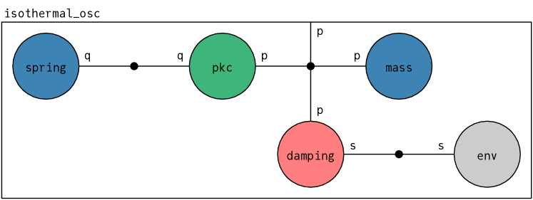
Figure 4: Interconnection pattern of an isothermal oscillator model. The box $\mathtt{pkc}$ represents the coupling of the potential energy domain represented by the junction on its left and the kinetic energy domain represented by the junction on its right. The box $\mathtt{env}$ represents the isothermal environment which absorbs the heat that is generated by the damping. The port $\mathtt{p}$ of the outer box exposes the kinetic energy domain, allowing for an external forcing of the oscillator model.

Figure 4 shows an interconnection pattern. The mathematical content of such a diagram is captured by the following definition:

Definition 3.1.

An interconnection pattern $(\beta,\,I,\,J)$ is defined by the following data:

1. A package of interfaces $\beta\in\mathbf{Pkg}(\mathbf{Interface})$. Names in $\operatorname{dom}(\beta)$ refer to inner boxes, $\sum\beta$ is called inner interface and names in $\operatorname{dom}(\sum\beta)$ refer to inner ports.

2. An interface $I$ called outer interface with ports called outer ports.

3. A partition $J$ of the combined interface $P=\sum\left[\mathtt{inner}\mapsto\sum\beta,\,\mathtt{outer}\mapsto I\right]$ such that each subset or junction $j\in J$ contains

   • at least one inner port,

   • at most one outer port,

   • and all ports have the same associated quantity. ∎

Although the names of inner ports and outer ports are distinguished by a prefix, usually the namespaces of $\sum\beta$ and $I$ are already disjoint. We then abuse notation and simply write for instance $\mathtt{p}$ rather than $\mathtt{outer.p}$.

We graphically depict interconnection patterns as follows. Each element $b\in\operatorname{dom}(\beta)$ is the name of an inner box, which we draw as a circle. The ports of its interface $\beta(b)$ are drawn as lines emanating from the box. The ports of the outer interface $I$ are drawn as lines to the surrounding outer box. Each subset $j\in J$ corresponds to a junction drawn as a black dot. The elements of $j\subseteq P$ are precisely the connected ports. To avoid confusion, we recall that the identifier isothermal_osc written on the top left of the outer box refers to the entire pattern (akin to a function name), rather than just to the outer box (which similar to the return value of a function does not need a name).

The pattern from Figure 4 is redrawn in Figure 5, firstly to emphasize that the color of the inner boxes is merely an annotation hinting at the nature of the considered subsystems and secondly to introduce an abbreviated way of writing port names.

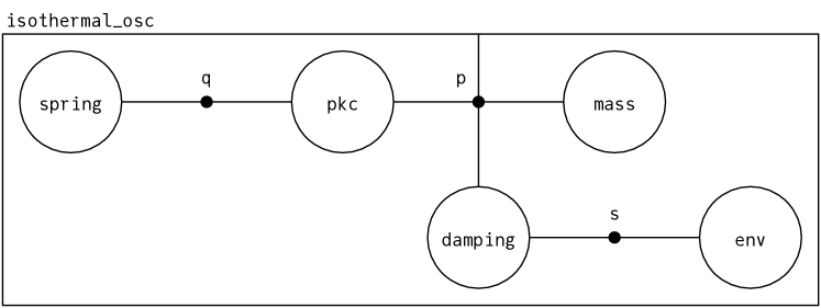
Figure 5: Interconnection pattern of an isothermal oscillator model. Whenever all ports connected to a certain junction have the same name we write the name only once at the junction.

Example 3.2.

For the pattern $(\beta,\,I,\,J)$ depicted in Figure 5, the namespace of inner boxes is

$$\operatorname{dom}(\beta)\>=\>\{\mathtt{spring},\,\mathtt{pkc},\,\mathtt{mass},\,\mathtt{damping},\,\mathtt{env}\}\,.$$

The function $\beta:\operatorname{dom}(\beta)\rightarrow\mathbf{Interface}$ is given by

$$\begin{split}\mathtt{spring}\>&\mapsto\>(\{\mathtt{q}\},\,\tau_{\text{spring}})\\ \mathtt{pkc}\>&\mapsto\>(\{\mathtt{q},\,\mathtt{p}\},\,\tau_{\text{pkc}})\\ \mathtt{mass}\>&\mapsto\>(\{\mathtt{p}\},\,\tau_{\text{mass}})\\ \mathtt{damping}\>&\mapsto\>(\{\mathtt{p},\,\mathtt{s}\},\,\tau_{\text{damping}})\\ \mathtt{env}\>&\mapsto\>(\{\mathtt{s}\},\,\tau_{\text{env}})\end{split}$$

with $\tau_{\text{spring}}(\mathtt{q})=((\mathbb{R},\,\mathtt{displacement}),\,\mathtt{p})$, etc. Hence, the namespace of the inner interface $\sum\beta$ is

$$\operatorname{dom}(\textstyle\sum\beta)\>=\>\{\mathtt{spring.q},\,\mathtt{pkc.q},\,\mathtt{pkc.p},\,\mathtt{mass.p},\,\mathtt{damping.p},\,\mathtt{damping.s},\,\mathtt{env.s}\}\,.$$

The namespace of the outer interface $I$ is $\{\mathtt{p}\}$. The partition $J$ is given by

$$\bigl{\{}\{\mathtt{spring.q},\,\mathtt{pkc.q}\},\,\{\mathtt{mass.p},\,\mathtt{pkc.p},\,\mathtt{damping.p},\,\mathtt{p}\},\,\{\mathtt{env.s},\,\mathtt{damping.s}\}\bigr{\}}\,.\qed$$

We may also denote an interconnection pattern using the condensed notation

In this we implicitly let $\operatorname{dom}(\beta)=\{\mathtt{I_{1}},\,\ldots,\,\mathtt{I_{n}}\}$ and $\beta(\mathtt{I_{i}})=I_{i}$. The left arrow is a surjection because each junction has at least one connected inner port and the right arrow is an injection because each junction has at most one connected outer port. Interconnection patterns are a special case of undirected wiring diagrams [37], which do not have the injectivity and surjectivity conditions.

As shown in Figure 1, interconnection patterns may have another feature that is not formalized by 3.1, namely port combinators for combining ports into multiports. Although namespaces seem to provide an adequate basis to formalize multiports and port combinators, we defer this to later work. At this point, we simply regard them as ad-hoc syntactic sugar for expressing parallel connections in a tidy and efficient manner.

3.2 Composition of interconnection patterns

Whenever the outer interface of one pattern and the interface corresponding to an inner box of another pattern are equivalent up to renaming of the ports, the former pattern can be substituted into the latter, with no further data required. This is called composition. Having a compositional syntax facilitates dealing with complex systems, as it allows to encapsulate subsystems, which can be easily reused and replaced, as long as interfaces match. As an example, the isothermal oscillator model can be refined into a nonisothermal oscillator model by substituting a more detailed damper model.

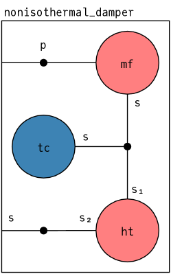
Figure 6: Interconnection pattern of a nonisothermal damper model. The box $\mathtt{mf}$ represents a mechanical friction model connected to the kinetic energy domain represented by the outer port $\mathtt{p}$. The box $\mathtt{tc}$ represents a thermal capacity, which can store the heat generated by friction. The box $\mathtt{ht}$ represents a heat transfer model, which allows the thermal capacity to reach equilibrium with the thermal energy domain represented by the outer port $\mathtt{s}$.

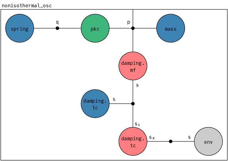
Figure 7: Interconnection pattern of a nonisothermal oscillator model.

Substituting the pattern in Figure 6 into the pattern in Figure 5, yields the pattern in Figure 7. Graphically, the former pattern is inserted into the inner box called $\mathtt{damping}$ of the latter pattern. In this step, the named sum for interfaces is used. Then, the common interface is deleted and for each of its ports, the two assigned junctions are identified.

Category theory provides a language to talk about composition and it includes well-behavedness conditions, which ensure that composition works in the way we expect, just as we need not worry about the difference between $(1+2)+1$ and $1+(2+1)$. In a following paper, we will formalize this using the language of operads.

4 Semantics of interconnection patterns

In this section, we discuss how to interpret an interconnection pattern as imposing a relation between the port variables of its inner and outer interface. We do this in two parts. In the first part, we talk about the relation as a collection of equations and discuss its physical interpretation. In the second part, we reify it as a geometric object, namely as a relation between bundles of port variables.

4.1 Interconnection patterns as equations

Informally, the semantics of an interconnection pattern $(\beta,\,I,\,J)$ can be seen as a collection of equations. Specifically, for each junction $j\in J$, we have the following:
Let $j_{p}\subseteq j$ be the subset of connected power ports.

• Equality of state. For all ports $p,p^{\prime}\in j$,

  $$p\mathtt{.x}\>=\>p^{\prime}\mathtt{.x}$$

• Equality of effort. For all power ports $p,p^{\prime}\in j_{p}$,

  $$p\mathtt{.e}\>=\>p^{\prime}\mathtt{.e}$$

• Equality of net flow.

  $$\sum_{p\,\in\,j_{p}\cap\sum\beta}p\mathtt{.f}\>=\>\sum_{p\,\in\,j_{p}\cap I}p\mathtt{.f}$$

As detailed in Section 7, combining these equations with equations that determine the semantics of each of the subsystems filling the inner boxes yields a collection of equations that determines the semantics of the resulting composite system.

Since all ports connected to a junction have the same quantity, their associated state variables take values in the same space, making equality of state a well-typed equation. As a consequence of equality of state, all effort variables take values in the same fiber of the same cotangent bundle, making equality of effort also well-typed. Similarly, all flow variables take values in the same fiber of the same tangent bundle, making equality of net flow well-typed.

Also note that in the equality of net flow, the inner ports are on the left hand side and the outer ports are on the right hand side. As a consequence, at every junction $j\in J$ the following power balance equation is satisfied:

$$\sum_{p\,\in\,j_{p}\cap\sum\beta}\langle p\mathtt{.e}\mid p\mathtt{.f}\rangle\>=\>\sum_{p\,\in\,j_{p}\cap I}\langle p\mathtt{.e}\mid p\mathtt{.f}\rangle$$

Summing over all junctions on both sides, we get that the net power supplied to all subsystems is equal to the net power supplied to the composite system. Taking into account also the choice of a sign made in Sections 6.1 and 6.2, we see that this agrees with the sign convention used in thermodynamics, stating that power supplied to any system, be it a subsystem or the composite system, is counted with a positive sign.

Junctions correspond to energy domains. Hence, an outer port exposes an energy domain of the respective composite system. Since this interpretation also applies to the primitive systems discussed in Section 6, we can say that ports also represent energy domains and whenever two ports are connected to the same junction the energy domains are identified. In other words, interconnection means that systems share common energy domains. The state of a shared energy domain is given by the shared state variable, according to the equality of state. The connected systems may exchange the respective physical quantity according to the equality of net flow. Moreover, such an exchange also implies an exchange of energy, according to the equality of effort.

Example 4.1.

Let’s again consider the pattern in Figure 7. At the junction representing the kinetic energy domain, the momentum variable (state) is shared and forces (flows) balance at equal velocity (effort):

$$\begin{aligned} &\mathtt{pkc.p.x}\>{}={}\>&&\mathtt{mf.p.x}\>{}={}\>&&\mathtt{mass.p.x}\>{}={}\>\mathtt{p.x}\\ &\mathtt{pkc.p.f}\>{}+{}\>&&\mathtt{mf.p.f}\>{}+{}\>&&\mathtt{mass.p.f}\>{}={}\>\mathtt{p.f}\\ &\mathtt{pkc.p.e}\>{}={}\>&&\mathtt{mf.p.e}\>{}={}\>&&\mathtt{mass.p.e}\>{}={}\>\mathtt{p.e}\end{aligned}\qed$$

Table 1 summarizes the physical interpretation of junctions representing a number of different energy domains.

energy domain	state variable	flows balance at equal efforts
kinetic	momentum	forces balance at equal velocity
magnetic	flux linkage	voltages balance at equal current
potential	displacement	velocities balance at equal force
hydraulic	volume	volume rates balance at equal pressure
electric	charge	currents balance at equal voltage
thermal	entropy	entropy rates balance at equal temperature

Table 1: Physical interpretation of junctions as energy domains.

We can now briefly reconsider the surjectivity and injectivity conditions which distinguish interconnection patterns form undirected wiring diagrams. The surjectivity condition says that each junction must have at least one connected inner port. In other words, an energy domain of the composite system must belong to at least one of its subsystems. Of course, an energy domain that is not part of the system cannot be exposed. The injectivity condition says that each junction may have at most one connected outer port. In other words, an energy domain can be exposed at most once. Exposing an energy domain twice and identifying it again at a higher level of nesting by connecting the two respective ports would lead to ill-defined flow variables.

4.2 Interconnection patterns as relations

Recall that a relation $R:A\nrightarrow B$ between two sets $A$ and $B$ is given by a subset of their Cartesian product, i.e. $R\subseteq A\times B$. Note that we are slightly abusing notation by reusing the symbol, here $R$, for the relation and the subobject by which it is defined. The arrow symbol $\nrightarrow$ should suggest that relations have no inherent direction, however the formal direction is relevant to denote their composition and hence to think about relations as forming a category.

Similarly to this prototypical example, the relation assigned to an interconnection pattern is given by a subbundle of the Cartesian product of the two bundles of port variables associated to the inner and the outer interface.

Definition 4.2.

Let $P=(\beta,\,I,\,J)$ be an interconnection pattern and let $I_{\text{in}}=\sum\beta$ denote its inner interface. Further, let $\mathcal{P}_{I_{\text{in}}}\twoheadrightarrow\mathcal{X}_{I_{\text{in}}}$ be the bundle of port variables associated to the inner interface and let $\mathcal{P}_{I}\twoheadrightarrow\mathcal{X}_{I}$ be the bundle of port variables associated to the outer interface. Based on the partition $J$, let $\mathcal{P}_{P}\subset\mathcal{P}_{I_{\text{in}}}\times\mathcal{P}_{I}$ be the subspace where equality of state, equality of effort, and equality of net flow are satisfied. Similarly, let $\mathcal{X}_{P}\subset\mathcal{X}_{I_{i}}\times\mathcal{X}_{I}$ be the subspace where equality of state is satisfied. Then, the semantics assigned to interconnection pattern $P$ is the relation $\mathcal{P}_{P}:\mathcal{P}_{I_{\text{in}}}\nrightarrow\mathcal{P}_{I}$ between the port variables of the inner interface and the port variables of the outer interface that is given by the vector subbundle $\mathcal{P}_{P}\twoheadrightarrow\mathcal{X}_{P}$. ∎

It can be shown that this assignment of semantics is functorial, which means that it makes no difference whether one first composes some interconnection patterns and then asks for the relation assigned to the composite or one first asks for the relations assigned to the original patterns and then composes these relations.

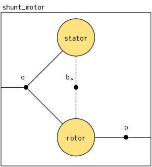
Figure 8: Interconnection pattern of a DC shunt motor model. The stator and rotor are connected to a common electric energy domain that is exposed via the outer port $\mathtt{q}$. The kinetic energy domain of the rotor is exposed via the outer port $\mathtt{p}$. The conversion between electric and kinetic energy in the rotor depends on the magnetic energy domain of the stator, which is represented by the junction with connected state ports named $\mathtt{b_{k}}$. The full model is discussed in Section 9.

Example 4.3.

Consider the interconnection pattern $P=(\beta,\,I,\,J)$ depicted in Figure 8 with names of inner boxes given by $\operatorname{dom}(\beta)=\{\mathtt{stator},\,\mathtt{rotor}\}$ and interfaces given by

$$\beta(\mathtt{stator})\>=\>\left(\{\mathtt{q},\,\mathtt{b_{s}}\},\,\tau_{\text{s}}\right)$$

$$\beta(\mathtt{rotor})\>=\>\left(\{\mathtt{q},\,\mathtt{p},\,\mathtt{b_{s}}\},\,\tau_{\text{r}}\right)$$

$$I\>=\>\left(\{\mathtt{q},\,\mathtt{p}\},\,\tau\right)\,,$$

where

$$\tau_{\text{s}}(\mathtt{q})\>=\>\tau_{\text{r}}(\mathtt{q})\>=\>\tau(\mathtt{q})\>=\>((\mathbb{R},\,\mathtt{charge}),\,\mathsf{p})$$

$$\tau_{\text{s}}(\mathtt{b_{s}})\>=\>\tau_{\text{r}}(\mathtt{b_{s}})\>=\>((\mathbb{R},\,\mathtt{flux\_linkage}),\,\mathsf{s})$$

$$\tau_{\text{r}}(\mathtt{p})\>=\>\tau(\mathtt{p})\>=\>((\mathbb{R},\,\mathtt{angular\_momentum}),\,\mathsf{p})\,.$$

Furthermore, the interconnection is determined by

$$J\>=\>\bigl{\{}\{\mathtt{stator.q},\,\mathtt{rotor.q},\,\mathtt{q}\},\,\{\mathtt{stator.b_{s}},\,\mathtt{rotor.b_{s}}\},\,\{\mathtt{rotor.p},\,\mathtt{p}\}\bigr{\}}\,.$$

The port space of the inner interface $I_{\text{in}}=\sum\beta$ is

$$\begin{split}\mathcal{P}_{I_{\text{in}}}\>=\>&\mathbb{T}\mathbb{R}\times\mathbb{R}\times\mathbb{T}\mathbb{R}\times\mathbb{T}\mathbb{R}\times\mathbb{R}\\ \>\ni\>&\bigl{(}(\mathtt{stator.q.x},\,\mathtt{stator.q.f},\,\mathtt{stator.q.e}),\,\mathtt{stator.b_{s}.x},\,\\ &\>\>(\mathtt{rotor.q.x},\,\mathtt{rotor.q.f},\,\mathtt{rotor.q.e}),\,\\ &\>\>(\mathtt{rotor.p.x},\,\mathtt{rotor.p.f},\,\mathtt{rotor.p.e}),\,\mathtt{rotor.b_{s}.x}\bigr{)}\end{split}$$

and the port space of the outer interface $I$ is

$$\mathcal{P}_{I}\>=\>\mathbb{T}\mathbb{R}\times\mathbb{T}\mathbb{R}\>\ni\>\bigl{(}(\mathtt{q.x},\,\mathtt{q.f},\,\mathtt{q.e}),\,(\mathtt{p.x},\,\mathtt{p.f},\,\mathtt{p.e})\bigr{)}\,.$$

Finally, the subspace $\mathcal{P}_{P}\subset\mathcal{P}_{I_{\text{in}}}\times\mathcal{P}_{I}$ defining the relation is

$$\begin{split}\mathcal{P}_{P}\>=\>\bigl{\{}\bigl{(}&(\mathtt{stator.q.x},\,\mathtt{stator.q.f},\,\mathtt{stator.q.e})\,,\,\mathtt{stator.b_{s}.x}\,,\,\\ &(\mathtt{rotor.q.x},\,\mathtt{rotor.q.f},\,\mathtt{rotor.q.e})\,,\,\\ &(\mathtt{rotor.p.x},\,\mathtt{rotor.p.f},\,\mathtt{rotor.p.e})\,,\,\mathtt{rotor.b_{s}.x}\,,\,\\ &(\mathtt{q.x},\,\mathtt{q.f},\,\mathtt{q.e})\,,\,(\mathtt{p.x},\,\mathtt{p.f},\,\mathtt{p.e})\bigr{)}\in\mathcal{P}_{I_{i}}\times\mathcal{P}_{I}\,\mid\,\\ &\mathtt{stator.q.x}=\mathtt{rotor.q.x}=\mathtt{q.x}\,,\,\\ &\mathtt{stator.q.e}=\mathtt{rotor.q.e}=\mathtt{q.e}\,,\,\\ &\mathtt{stator.q.f}+\mathtt{rotor.q.f}=\mathtt{q.f}\,,\,\\ &\mathtt{stator.b_{s}.x}=\mathtt{rotor.b_{s}.x}\,,\,\\ &\mathtt{rotor.p.x}=\mathtt{p.x}\,,\,\\ &\mathtt{rotor.p.e}=\mathtt{p.e}\,,\,\\ &\mathtt{rotor.p.f}=\mathtt{p.f}\,\bigr{\}}\,.\qed\end{split}$$

5 Exergy

Every system is ultimately determined by a power-preserving interconnection of primitive subsystems, also called components, which represent elementary physical behaviors such as storage and reversible as well as irreversible exchange of energy. To achieve a thermodynamically consistent combination of reversible and irreversible dynamics, components are defined with respect to a fixed exergy reference environment that is discussed in this section.

5.1 Intuition

As briefly discussed in Section 1.4, thermodynamic models do not have all their physically-relevant degrees of freedom determined by their state variables, which leads to irreversibility. According to the first and second law of thermodynamics, internal energy, which is given by an imprecise phenomenological description, cannot be fully converted into mechanical or electromagnetic energy, which is precise, in the sense that the relevant degrees of freedom are determined by the state variables.

The irreversible degradation of ‘mechanically precise’ forms of energy into ‘thermodynamically imprecise’ forms of energy can be quantified using the concept of exergy. A hypothetical conversion device, whose mode of operation is only restricted by the first and second law of thermodynamics is used to determine how much mechanical (or electromagnetic) energy can be extracted from a system before it reaches thermodynamic equilibrium with a reference environment, whose intensive variables, such as temperature and pressure, are constant (in time and space), see Figure 9.

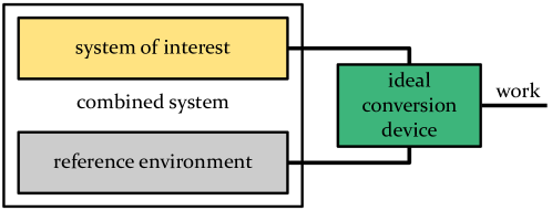
Figure 9: To assess the exergy content of a system, it is combined with a reference environment. The exergy content is then defined as the maximum amount of work that can be extracted from the combined system via a hypothetical conversion device that operates completely reversibly.

Crucially, the ideal conversion device is not restricted to interacting with the system through its interface. Instead, the device operates in a counterfactual where all energy domains of both the system and the environment can be accessed. This means that the exergy content of a (hierarchically flattened) composite system can be obtained by summing the exergy stored in each of its storage components. So, in particular, the exergy content of a system does not depend on how its subsystems are interconnected. The exergy content of a component storing internal energy is assessed based on an ideal conversion device and the reference environment, while the exergy content of a component storing only mechanical or electromagnetic forms of energy is equal to its energy content.

As also remark that a similar concept of available energy could be defined intrinsically, meaning without relying on a reference environment. The reversible conversion device would then interact only with the system of interest until it reaches equilibrium with itself. However, the use of a reference environment with fixed intensive quantities has the important advantage that the exergy content of a system is given explicitly by its exergy storage function, which follows systematically from its energy storage function and the definition of the reference environment, as detailed in Section 6.1. In contrast, the intrinsic concept in general would lead to an optimization problem without a simple closed-form solution.

More information and references about exergy, its history, and its links to port-Hamiltonian as well as GENERIC systems can be found in [20].

5.2 Reference environment

Definition 5.1.

A reference environment $(I_{R},\,\lambda_{R})$ is given by an interface $I_{R}=(N_{R},\,\tau_{R})$ such that each port $p\in I_{R}$ is a power port with an unique extensive quantity in $\mathbf{Q}_{\mathbb{R}}$ and an associated value $\lambda_{R}(p)\in\mathbb{R}^{*}$ of the energy-conjugate intensive quantity. ∎

Uniqueness of quantities, i.e. injectivity of $\tau_{R}:N_{R}\rightarrow\mathbf{Q}_{\mathbb{R}}\times\{\mathsf{p}\}$, is required to determine the exergy storage function of a system from its energy storage function. Regarding the physical interpretation, each port corresponds to an energy domain that is present in the environment. Allowing multiple energy domains of the same kind would conflict with the environment always being in equilibrium with itself.

Example 5.2.

The minimal definition of a reference environment represents an isothermal heat bath. This amounts to an interface with a single entropy port and an associated reference temperature, henceforth denoted by ${\color[rgb]{.5,0,.5}\theta_{0}}$:

$$N_{R} =\>\{\mathtt{s}\}$$

$$\tau_{R}(\mathtt{s}) =\>\left((\mathbb{R},\,\mathtt{entropy}),\,\mathsf{p}\right)$$

$$\lambda_{R}(\mathtt{s}) =\>{\color[rgb]{.5,0,.5}\theta_{0}}\>=\>$298.15\text{\,}\mathrm{K}$\,.$$

To determine the exergy content of pressurized fluids with respect to an isobaric atmosphere, the definition of the environment can be extended to $N_{R}=\{\mathtt{s},\,\mathtt{v}\}$ with

$$\tau_{R}(\mathtt{v}) =\>\left((\mathbb{R},\,\mathtt{volume}),\,\mathsf{p}\right)$$

$$\lambda_{R}(\mathtt{v}) =\>{\color[rgb]{.5,0,.5}-\pi_{0}}\>=\>$-1013.25\text{\,}\mathrm{hPa}$\,.$$

The minus sign in front of the reference pressure ${\color[rgb]{.5,0,.5}\pi_{0}}$ stems from the fact that more volume means less energy. To model for instance a mass diffusion process, a port $\mathtt{m}$ representing the mass of a chemical species with a fixed chemical potential ${\color[rgb]{.5,0,.5}\mu_{0}}$ should be included, i.e. let $N_{R}=\{\mathtt{s},\,\mathtt{v},\,\mathtt{m}\}$ with

$$\begin{aligned} \tau_{R}(\mathtt{m})\>&=\>\left((\mathbb{R},\,\mathtt{mass}),\,\mathsf{p}\right)\\ \lambda_{R}(\mathtt{m})\>&=\>{\color[rgb]{.5,0,.5}\mu_{0}}\,.\end{aligned}\qed$$

A software implementation should include a comprehensive definition of a reference environment and allow the user to redefine the values of the intensive quantities.

6 Primitive systems

The lowest level of any hierarchical model specification is defined by primitive systems, also called components. There are four classes of components:

• Storage components represent energy storage.

• Reversible components represent reversible energy exchange
  (or a transformation between different forms of describing an energy domain).

• Irreversible components represent irreversible energy exchange.

• Environment components are used to model energy exchange with
  the reference environment.

Components are in general defined with respect to a reference environment $(I_{R},\,\lambda_{R})$. Further, every component has an interface $I=(N,\,\tau)$ with port variables $(x,\,f,\,e)\in\mathcal{P}_{I}$. To define the exergy storage function of storage components and to state fundamental thermodynamic properties of reversible as well as irreversible components, we define the following notation: For any port $p\in I$, let

$$\lambda(p)\>=\>\begin{cases}\lambda_{R}(p_{R})&\exists\,p_{R}\in I_{R}\,\colon\,\tau_{R}(p_{R})\>=\>\tau(p)\\ 0\in\mathrm{T}^{*}\mathcal{X}_{p}&\text{else.}\end{cases}$$

For instance, if $p$ represents a thermal energy domain then $\lambda(p)={\color[rgb]{.5,0,.5}\theta_{0}}$, whereas if $p$ represents a kinetic energy domain then $\lambda(p)=0$, since the environment does not have a kinetic energy domain. This can also be applied to the entire interface. E.g. for $N=\{\mathtt{p_{1}},\,\ldots,\,\mathtt{p_{n}}\}$, let

$$\lambda(I)\>=\>\bigl{(}\lambda(\mathtt{p_{1}}),\,\ldots,\,\lambda(\mathtt{p_{n}})\bigr{)}\,.$$

We also define a similar notation that references a specific environment port: For any port $p\in I$ and $p_{R}\in I_{R}$, let

$$\lambda(p,\,p_{R})\>=\>\begin{cases}\lambda_{R}(p_{R})&\tau_{R}(p_{R})\>=\>\tau(p)\\ 0\in\mathrm{T}^{*}\mathcal{X}_{p}&\text{else.}\end{cases}$$

Again, given e.g. $N=\{\mathtt{p_{1}},\,\ldots,\,\mathtt{p_{n}}\}$, let

$$\lambda(I,\,p_{R})\>=\>\bigl{(}\lambda(\mathtt{p_{1}},\,p_{R}),\,\ldots,\,\lambda(\mathtt{p_{n}},\,p_{R})\bigr{)}\,.$$

6.1 Storage components

Storage components are primitive systems representing energy storage. Examples include elastic springs, movable masses, capacitors, inductors, and thermal capacities.

Definition 6.1.

A storage component $(I,\,E)$ is defined by an interface $I$ containing only power ports and an energy storage function $E:\mathcal{X}_{I}\rightarrow\mathbb{R}$. ∎

The function $E$ simply yields the stored energy for any state $x\in\mathcal{X}_{I}$. Based on the reference environment $I_{R}$, the exergy content is determined as follows.

Definition 6.2.

Let $(I,\,E)$ be a storage component. Its exergy storage function $H:\mathcal{X}_{I}\rightarrow\mathbb{R}$ is given by

$$H(x)\>=\>E(x)-\sum_{p\,\in\,I}\sum_{\begin{subarray}{c}p_{R}\,\in\,I_{R}\\ \tau_{R}(p_{R})\,=\,\tau(p)\end{subarray}}\langle\lambda_{R}(p_{R})\mid p\mathtt{.x}\rangle\,.\qed$$

Note that in the natural pairing, $\mathbb{R}$ is implicitly identified with its tangent space, i.e. $\mathbb{R}\cong\mathrm{T}_{p\mathtt{.x}}\mathbb{R}$. While the exergy content of a system is supposed to be zero when it reaches equilibrium with itself and the environment, the component-wise definition for EPHS may yield another minimum value for the total exergy. In this case, a constant may be added to remedy this. Regarding the dynamics of the system, this is however irrelevant, as it depends only on the differential $\differential H$. Specifically, the effort variables are given by the differential of the exergy function evaluated at the current state $x\in\mathcal{X}_{I}$:

$$\forall\,p\in I\>:\>p\mathtt{.e}\>=\>\left.\partialderivative{H}{(p\mathtt{.x})}\right|_{x}$$

In case the constant offset should matter for thermodynamic analysis, it can be added to the total exergy function once the equilibrium state of the system under study has been determined. Finally, the trajectory of the state variables is obtained by integrating the flow variables:

$$\forall\,p\in I\>:\>\derivative{(p\mathtt{.x})}{t}\>=\>p\mathtt{.f}$$

Example 6.3.

Consider a storage component $(I_{\text{gas}},\,E_{\text{gas}})$ representing a gas-filled compartment whose entropy and volume can change. Its interface $I_{\text{gas}}$ is defined as in 2.18 and we assume knowledge of its energy storage function $E_{\text{gas}}:\mathbb{R}\times\mathbb{R}\rightarrow\mathbb{R}$. Writing $x=(s,\,v)$, the exergy storage function is then given by

$$H_{\text{gas}}(s,\,v)\>=\>E_{\text{gas}}(s,\,v)\,-\,{\color[rgb]{.5,0,.5}\theta_{0}}\,s\,+\,{\color[rgb]{.5,0,.5}\pi_{0}}\,v\,.$$

With the temperature being defined as $\theta=\partialderivative{E_{\text{gas}}}{s}$ and the negative pressure being defined as $-\pi=\partialderivative{E_{\text{gas}}}{v}$, the effort variables are given by

$$\begin{split}\mathtt{s.e}\>&=\>\theta-{\color[rgb]{.5,0,.5}\theta_{0}}\\ \mathtt{v.e}\>&=\>-(\pi-{\color[rgb]{.5,0,.5}\pi_{0}})\,.\end{split}$$

Since the entropy rate $\dot{s}=\mathtt{s.f}$ is related to the heat flow rate $\Phi$ via $\dot{s}=\frac{1}{\theta}\,\Phi$, the exergetic power at the entropy port is $\langle\mathtt{s.e}\mid\mathtt{s.f}\rangle=\frac{\theta-{\color[rgb]{.5,0,.5}\theta_{0}}}{\theta}\,\Phi=\eta_{\text{Carnot}}\,\Phi$, where $\eta_{\text{Carnot}}$ is the efficiency of an ideal heat engine operating between a hot source with temperature $\theta$ and a cold sink with temperature ${\color[rgb]{.5,0,.5}\theta_{0}}$. Considering a piston with the pressurized gas on one side and the atmosphere on the other, $\langle\mathtt{v.e}\mid\mathtt{v.f}\rangle=-(\pi-{\color[rgb]{.5,0,.5}\pi_{0}})\,\dot{v}$ is the power that can be extracted from the pressurized gas when its volume grows at rate $\dot{v}$. ∎

Next, we define the semantics of a storage component with interface $I$ in terms of a relation $\mathcal{S}:\mathrm{T}\mathcal{X}_{I}\nrightarrow\mathcal{P}_{I}$. This is used in Section 7, where we define the semantics of a composite system in terms of the semantics of its primitive subsystems and the semantics of its (hierarchy of nested) interconnection pattern(s).

Definition 6.4.

The semantics assigned to storage component $(I,\,E)$ is the relation $\mathcal{S}:\mathrm{T}\mathcal{X}_{I}\nrightarrow\mathcal{P}_{I}$ that is given by the subbundle

$$\mathcal{S}\>=\>\bigl{\{}\bigl{(}(\tilde{x},\,\tilde{f}),\,(x,\,f,\,e)\bigr{)}\in\mathrm{T}\mathcal{X}_{I}\times\mathcal{P}_{I}\,\mid\,\tilde{x}\>=\>x,\,\tilde{f}\>=\>f,\,e\>=\>\differential H(x)\bigr{\}}\,,$$

where $H$ is induced from $E$ according to 6.2. ∎

6.2 Environment components

While the primary role of the reference environment is to enable the thermodynamically consistent combination of reversible and irreversible dynamics, it may also be represented by a component to model energy exchange with the environment. For instance, an environment component can represent an isothermal heat bath, which may absorb heat generated by irreversible components, or an isobaric atmosphere, which may exchange pressure-volume work with other components.

Definition 6.5.

An environment component is defined by a subinterface $I\subseteq I_{R}$ containing the exposed energy domains of the reference environment. ∎

The state variables keep track of the exchanged entropy, volume, etc. As for storage components, their rate of change is given by the flow variables:

$$\forall\,p\in I\>:\>\derivative{(p\mathtt{.x})}{t}\>=\>p\mathtt{.f}$$

Since the exergy content of the environment is zero by definition, the effort variables are also zero:

$$\forall\,p\in I\>:\>p\mathtt{.e}\>=\>0$$

Consequently, the semantics of an environment component is assigned as follows:

Definition 6.6.

The semantics assigned to environment component $I\subseteq I_{R}$ is the relation $\mathcal{E}:\mathrm{T}\mathcal{X}_{I}\nrightarrow\mathcal{P}_{I}$ that is given by the subbundle

$$\mathcal{E}\>=\>\bigl{\{}\bigl{(}(\tilde{x},\,\tilde{f}),\,(x,\,f,\,e)\bigr{)}\in\mathrm{T}\mathcal{X}_{I}\times\mathcal{P}_{I}\,\mid\,\tilde{x}\>=\>x,\,\tilde{f}\>=\>f,\,e\>=\>0\bigr{\}}\,.\qed$$

6.3 Reversible components

In a generalized sense, reversible components represent gyrators, transformers, and/or kinematic constraints. Generalized gyrators describe the reversible coupling of different kinds of energy domains, such as a coupling of kinetic and potential energy domains in mechanics or an electro-magnetic coupling. Examples where one domain reversibly interacts with itself are gyroscopic forces in rigid body dynamics and self-advection of kinetic energy in fluid dynamics. The Lorentz force is another example where a kinetic energy domain interacts with itself in a way that depends on the state of a magnetic energy domain. Generalized transformers couple energy domains of the same kind. They may for instance represent mechanical levers or ideal electrical transformers. Frame transformations in multibody systems present an example where a transformation between different representations of the same energy domain is realized. Examples of kinematic constraints include joint constraints in multibody dynamics and the incompressibility constraint in fluid dynamics. Further, the parallel connection of capacitors, the series connection of inductors or springs, as well as rigid links between point masses are described by constraints.

The geometric structure behind reversible components is called Dirac structure. For our purposes, an (almost) Dirac structure $\mathcal{D}$ is a power-preserving, locally linear relation of port variables. More precisely, we could define $\mathcal{D}\subset\mathcal{P}_{I}$ as a maximally isotropic vector subbundle of the bundle of port variables $\mathcal{P}_{I}\twoheadrightarrow\mathcal{X}_{I}$, see [1, 49, 13]. However, to state fundamental properties of reversible components, we give a more practical definition of Dirac structures in terms of a particular representation, which may be called constrained hybrid input-output representation (cf. [13]):

Definition 6.7.

Let $I$ be an interface and let $\mathcal{X}_{I,p}\cong\mathcal{X}_{1}\times\mathcal{X}_{2}\ni x_{p}=(x_{1},\,x_{2})$ be a factorization of the state space of its power ports with flow and effort variables correspondingly denoted by $f=(f_{1},\,f_{2})$ and $e=(e_{1},\,e_{2})$. A Dirac structure $\mathcal{D}\subset\mathcal{P}_{I}$ admits the following representation:

$$\mathcal{D}\,=\,\left\{(x,\,f,\,e)\in\mathcal{P}_{I}\,\mid\,\exists\,\lambda_{c}\in V^{*}\,\colon\left[\begin{array}[]{c}f_{1}\\ \hline\cr e_{2}\\ \hline\cr 0\end{array}\right]\,=\,\left[\begin{array}[]{c | c | c}L(x)&-g(x)&C^{*}(x)\\ \hline\cr g^{*}(x)&0&0\\ \hline\cr-C(x)&0&0\end{array}\right]\,\left[\begin{array}[]{c}e_{1}\\ \hline\cr f_{2}\\ \hline\cr\lambda_{c}\end{array}\right]\right\}$$

Here, $L:\mathrm{T}^{*}\mathcal{X}_{1}\rightarrow\mathrm{T}\mathcal{X}_{1}$, $g:\mathrm{T}\mathcal{X}_{2}\rightarrow\mathrm{T}\mathcal{X}_{1}$, its linear dual $g^{*}:\mathrm{T}^{*}\mathcal{X}_{1}\rightarrow\mathrm{T}^{*}\mathcal{X}_{2}$, $C:\mathrm{T}^{*}\mathcal{X}_{1}\rightarrow\mathcal{X}_{I}\times V$, and its dual $C^{*}:\mathcal{X}_{I}\times V^{*}\rightarrow\mathrm{T}\mathcal{X}_{1}$ are vector bundle maps over the identity on $\mathcal{X}_{I}$. Further, $V$ is a vector space and $L(x)$ is skew-symmetric for all $x\in\mathcal{X}_{I}$. ∎

The maps $L$, $g$ and $C$ define a gyrator, a transformer and a constraint, respectively. The constraint is enforced via the Lagrange multiplier $\lambda_{c}$. Due to the skew-symmetry of the matrix in 6.7, exergetic power is conserved, i.e.

$$\langle e_{1}\mid f_{1}\rangle\>+\>\langle e_{2}\mid f_{2}\rangle\>=\>0\,.$$

Example 6.8.

Let the interface $I_{\text{hk}}=(N_{\text{hk}},\,\tau_{\text{hk}})$ be given by

$$\begin{split}N_{\text{hk}}\>&=\>\{\mathtt{v_{1}},\,\mathtt{v_{2}},\,\mathtt{p}\}\\ \tau_{\text{hk}}(\mathtt{v_{1}})\>&=\>\tau_{\text{hk}}(\mathtt{v_{2}})\>=\>((\mathbb{R},\,\mathtt{volume}),\,\mathsf{p})\\ \tau_{\text{hk}}(\mathtt{p})\>&=\>((\mathbb{R},\,\mathtt{momentum}),\,\mathsf{p})\end{split}$$

and let $a\in\mathbb{R}$ be a constant surface area of a piston. Then, the following equation defines a Dirac structure $\mathcal{D}_{\text{hk}}\subset\mathcal{P}_{I_{\text{hk}}}$:

$$\left[\begin{array}[]{c}\mathtt{v_{1}.f}\\ \mathtt{v_{2}.f}\\ \mathtt{p.f}\end{array}\right]\>=\>\left[\begin{array}[]{rrr}0&0&a\\ 0&0&-a\\ -a&a&0\end{array}\right]\,\left[\begin{array}[]{c}\mathtt{v_{1}.e}\\ \mathtt{v_{2}.e}\\ \mathtt{p.e}\end{array}\right]$$

This describes a generalized gyrator that couples the two hydraulic energy domains at the front and the back side of a piston with a kinetic energy domain corresponding to the piston’s moving mass. ∎

A reversible component is defined by a Dirac structure which satisfies two extra properties ensuring thermodynamic consistency.

Definition 6.9.

A reversible component $(I,\,\mathcal{D})$ is given by an interface $I$ and a Dirac structure $\mathcal{D}\subset\mathcal{P}_{I}$ such that all quantities of the reference environment are conserved and the time-reversal invariance property holds. The first condition requires that

$$\forall\,p_{R}\in I_{R}\>:\>\forall\,x\in\mathcal{X}_{I}\>:\>\Bigl{(}0\>=\>L(x)\,\lambda(I_{1},\,p_{R})\quad\text{and}\quad 0\>=\>g^{*}(x)\,\lambda(I_{1},\,p_{R})\Bigr{)}\,.$$

The time-reversal invariance property holds if $\forall\,x\in\mathcal{X}_{I}\,\colon$

$${(L(x))}^{ij}\neq 0 \implies- \mathrm{P}(x_{1}^{i})\> =\>\mathrm{P}({(L(x))}^{ij})\,\mathrm{P}(x_{1}^{j})$$

$${(g(x))}^{ik}\neq 0 \implies \mathrm{P}(x_{1}^{i})\> =\>\mathrm{P}({(g(x))}^{ik})\,\mathrm{P}(x_{2}^{k})\,.$$

Here, we use abstract index notation without implied summation. Indices $i$ and $j$ range over the power ports associated with $\mathcal{X}_{1}$ and $k$ ranges over the power ports associated with $\mathcal{X}_{2}$. The state variable is accordingly split as $x=(x_{p},\,x_{s})=((x_{1},\,x_{2}),\,x_{s})$ and $\mathrm{P}$ yields the parity of the respective quantity with $\mathrm{P}(\mathrm{const.})=+1$. ∎

Example 6.10.

The reversible component $(I_{\text{hk}},\,\mathcal{D}_{\text{hk}})$, as already defined in 6.8, describes the coupling between the kinetic energy domain of a piston with surface area $a$ and the two hydraulic energy domains on either side of the piston. The first condition here ensures that volume is conserved. This is satisfied since

$$\left[\begin{array}[]{c}0\\ 0\\ 0\end{array}\right]\>=\>\left[\begin{array}[]{rrr}0&0&a\\ 0&0&-a\\ -a&a&0\end{array}\right]\,\left[\begin{array}[]{c}{\color[rgb]{.5,0,.5}-\pi_{0}}\\ {\color[rgb]{.5,0,.5}-\pi_{0}}\\ 0\end{array}\right]\,.$$

The time-reversal invariance property holds since

$$\begin{split}-\mathrm{P}(\mathtt{(\mathbb{R},\,volume}))\>&=\>\mathrm{P}(a)\,\mathrm{P}((\mathbb{R},\,\mathtt{momentum}))\\ -\mathrm{P}((\mathbb{R},\,\mathtt{volume}))\>&=\>\mathrm{P}(-a)\,\mathrm{P}((\mathbb{R},\,\mathtt{momentum}))\,.\end{split}$$

Checks for the other two non-zero entries of $L$ must pass due to its skew-symmetry. ∎

The semantics of a reversible component is simply given by its Dirac structure interpreted as a relation:

Definition 6.11.

The semantics assigned to reversible component $(I,\,\mathcal{D})$ is the relation $\mathcal{D}:1\nrightarrow\mathcal{P}_{I}$ that is given by its Dirac structure $\mathcal{D}$. ∎

The symbol $1$ in $1\nrightarrow\mathcal{P}_{I}$ refers to the Cartesian unit for vector bundles, i.e. the vector bundle with a single point as its base space and the zero-dimensional vector space above it.

6.4 Irreversible components

Irreversible components are phenomenological models of irreversible processes with local thermodynamic equilibrium. Examples include mechanical friction, fluid viscosity, electrical conduction / resistance, thermal conduction, and mass diffusion. Such models can be defined in terms of a function that maps thermodynamic forces, which drive the relaxation process, to thermodynamic fluxes, which seek to restore equilibrium. Based on the assumption that the microscopic dynamics are reversible, Onsager found that such maps must satisfy a symmetry property [6]. This motivates our definition of an Onsager structure:

Definition 6.12.

Let $I$ be an interface. An Onsager structure $\mathcal{O}\subset\mathcal{P}_{I}$ is a fiber subbundle that admits the following representation:

$$\mathcal{O}\,=\,\left\{(x,\,f,\,e)\in\mathcal{P}_{I}\,\mid\,f\>=\>\frac{1}{\color[rgb]{.5,0,.5}\theta_{0}}\,M(e)\,e\right\}\,,$$

where $M$ is a smooth function that yields a symmetric non-negative definite linear operator $M(e)\colon\mathrm{T}^{*}\mathcal{X}_{I,p}\to\mathrm{T}\mathcal{X}_{I,p}$ for all effort variables $e\in\mathrm{T}^{*}\mathcal{X}_{I,p}$. ∎

In contrast to a Dirac structure, an Onsager structure is neither power-preserving, nor is it a locally linear relation of the port variables, since destruction of exergy, or equivalently production of entropy, is described in general by a non-linear relation. Hence, $\mathcal{O}\subset\mathcal{P}_{I}$ is not a vector subbundle of $\mathcal{P}_{I}$, but merely a fiber subbundle. The symmetry of $M(e)$ corresponds to Onsager’s reciprocal relations and its non-negative definiteness implies a non-negative exergy destruction rate.

Example 6.13.

Let the interface $I_{\text{mf}}=(N_{\text{mf}},\,\tau_{\text{mf}})$ be given by

$$\begin{split}N_{\text{mf}}\>&=\>\{\mathtt{p},\,\mathtt{s}\}\\ \tau_{\text{mf}}(\mathtt{p})\>&=\>((\mathbb{R},\,\mathtt{momentum}),\,\mathsf{p})\\ \tau_{\text{mf}}(\mathtt{s})\>&=\>((\mathbb{R},\,\mathtt{entropy}),\,\mathsf{p})\end{split}$$

and let $d\in\mathbb{R}_{>0}$ be a friction coefficient. Then, the following defines an Onsager structure $\mathcal{O}_{\text{mf}}\subset\mathcal{P}_{I_{\text{mf}}}$ representing mechanical friction:

$$\begin{bmatrix}\mathtt{p.f}\\ \mathtt{s.f}\end{bmatrix}\>=\>\frac{1}{\color[rgb]{.5,0,.5}\theta_{0}}\,d\,\begin{bmatrix}\theta&-\upsilon\\ -\upsilon&\frac{\upsilon^{2}}{\theta}\end{bmatrix}\,\begin{bmatrix}\mathtt{p.e}\\ \mathtt{s.e}\end{bmatrix}$$

Here, $\upsilon=\mathtt{p.e}$ is the velocity and $\theta={\color[rgb]{.5,0,.5}\theta_{0}}+\mathtt{s.e}$ is the absolute temperature at which kinetic energy is dissipated into the thermal energy domain. The phenomenological parameter $d$ could also be a function of the effort variables $e$, i.e. it could depend on the velocity and the temperature, or theoretically also the base point $x$. The above can be simplified to $\mathtt{p.f}=d\,\upsilon$ and $\mathtt{s.f}=-\frac{1}{\theta}\,d\,\upsilon^{2}$. Hence, the environment temperature ${\color[rgb]{.5,0,.5}\theta_{0}}$ cancels out in the flow variables, which here are the friction force and the entropy production rate (with a minus sign since thermal energy is leaving the component). ∎

An irreversible component is defined by an Onsager structure which satisfies two extra properties ensuring thermodynamic consistency:

Definition 6.14.

An irreversible component $(I,\,\mathcal{O})$ is given by an interface $I$ and an Onsager structure $\mathcal{O}\subset\mathcal{P}_{I}$ such that energy and all quantities of the reference environment, except for entropy, are conserved and the time-reversal invariance property does strictly not hold. The condition for conservation of energy requires that

$$\forall\,e\in\mathrm{T}^{*}\mathcal{X}_{I,p}\>:\>0\>=\>M(e)\,\bigl{(}\lambda(I)+e\bigr{)}\,.$$

The condition that all quantities of the reference environment, except for entropy, are conserved requires that

$$\forall\,p_{R}\in I_{R}\>:\>\Bigl{(}\tau_{R}(p_{R})\neq((\mathbb{R},\,\mathtt{entropy}),\,\mathsf{p})\implies\bigl{(}\forall\,e\in\mathrm{T}^{*}\mathcal{X}_{I,p}\>:\>0\>=\>M(e)\,\lambda(I,\,p_{R})\bigr{)}\Bigr{)}\,.$$

The time-reversal invariance property does strictly not hold if $\forall\,x\in\mathcal{X}_{I}\,\colon$

$${(M(x))}^{ij}\neq 0\implies\mathrm{P}(x^{i})\>=\>\mathrm{P}({(M(x))}^{ij})\,\mathrm{P}(x^{j})\,.$$

Here, we use the same notation as in 6.9 with indices $i$ and $j$ ranging over all power ports of $I$. ∎

Example 6.15.

The irreversible component $(I_{\text{mf}},\,\mathcal{O}_{\text{mf}})$, as already defined in 6.13, models mechanical friction. The condition for conservation of energy is satisfied since

$$\begin{bmatrix}0\\ 0\end{bmatrix}\>=\>d\,\begin{bmatrix}\theta&-\upsilon\\ -\upsilon&\frac{\upsilon^{2}}{\theta}\end{bmatrix}\,\begin{bmatrix}\upsilon\\ \theta\end{bmatrix}\,.$$

The condition that all quantities of the reference environment, except for entropy, are conserved is trivially satisfied. The time-reversal invariance property does strictly not hold since

$$\begin{split}\mathrm{P}((\mathbb{R},\,\mathtt{momentum}))\>&=\>\mathrm{P}(d)\,\mathrm{P}(\theta)\,\mathrm{P}((\mathbb{R},\,\mathtt{momentum}))\\ \mathrm{P}((\mathbb{R},\,\mathtt{momentum}))\>&=\>\mathrm{P}(d)\,\mathrm{P}(-\upsilon)\,\mathrm{P}((\mathbb{R},\,\mathtt{entropy}))\\ \mathrm{P}((\mathbb{R},\,\mathtt{entropy}))\>&=\>\mathrm{P}(d)\,\mathrm{P}(-\upsilon)\,\mathrm{P}((\mathbb{R},\,\mathtt{momentum}))\\ \mathrm{P}((\mathbb{R},\,\mathtt{entropy}))\>&=\>\mathrm{P}(d)\,{(\mathrm{P}(\upsilon))}^{2}\,/\,\mathrm{P}(\theta)\,\mathrm{P}((\mathbb{R},\,\mathtt{entropy}))\,,\end{split}$$

where we used that temperature has positive parity and velocity has negative parity. ∎

Example 6.16.

Let the interface $I_{\text{ht}}=(N_{\text{ht}},\,\tau_{\text{ht}})$ be given by

$$\begin{split}N_{\text{ht}}\>&=\>\{\mathtt{s_{1}},\,\mathtt{s_{2}}\}\\ \tau_{\text{ht}}(\mathtt{s_{1}})\>&=\>\tau_{\text{ht}}(\mathtt{s_{2}})\>=\>((\mathbb{R},\,\mathtt{entropy}),\,\mathsf{p})\,,\end{split}$$

let $\alpha\in\mathbb{R}_{>0}$ be a heat transfer coefficient, and let the Onsager structure $\mathcal{O}_{\text{ht}}\subset\mathcal{P}_{I_{\text{ht}}}$ be given by

$$\begin{bmatrix}\mathtt{s_{1}.f}\\ \mathtt{s_{2}.f}\end{bmatrix}\>=\>\frac{1}{\color[rgb]{.5,0,.5}\theta_{0}}\,\alpha\,\begin{bmatrix}\frac{\theta_{2}}{\theta_{1}}&-1\\ -1&\frac{\theta_{1}}{\theta_{2}}\end{bmatrix}\,\begin{bmatrix}\mathtt{s_{1}.e}\\ \mathtt{s_{2}.e}\end{bmatrix}\,,$$

where $\theta_{1}={\color[rgb]{.5,0,.5}\theta_{0}}+\mathtt{s_{1}.e}$ and $\theta_{2}={\color[rgb]{.5,0,.5}\theta_{0}}+\mathtt{s_{2}.e}$ are the absolute temperatures of the two thermal domains. Then, we can check that $(I_{\text{mf}},\,\mathcal{O}_{\text{mf}})$, defines an irreversible component. Again, the phenomenological parameter $\alpha$ could for instance be a function of the temperatures. The above can be simplified to $\mathtt{s_{1}.f}=-\frac{1}{\theta_{1}}\,\alpha\,(\theta_{2}-\theta_{1})$ and $\mathtt{s_{2}.f}=-\frac{1}{\theta_{2}}\,\alpha\,(\theta_{1}-\theta_{2})$. Hence, the environment temperature ${\color[rgb]{.5,0,.5}\theta_{0}}$ cancels out in the flow variables, which are rates of entropy change due to heat transfer. ∎

The semantics of an irreversible component is simply given by its Onsager structure interpreted as a relation:

Definition 6.17.

The semantics assigned to irreversible component $(I,\,\mathcal{O})$ is the relation $\mathcal{O}:1\nrightarrow\mathcal{P}_{I}$ that is given by its Onsager structure $\mathcal{O}$. ∎

7 Composite systems

A composite system is formed by interconnecting finitely many systems, be they primitive systems or other composite systems, according to an interconnection pattern. The data defining a composite system is therefore given by an interconnection pattern and for each of its inner boxes a system with the corresponding interface.

Definition 7.1.

Let $\mathbf{System}$ refer to the set of all systems defined with respect to a fixed reference environment. A composite system $(I,\,\gamma,\,J)$ is defined by the following data:

1. An interface $I$ of the composite system.

2. A package of systems $\gamma\in\mathbf{Pkg}(\mathbf{System})$, which can be reduced to a package of interfaces $\beta\in\mathbf{Pkg}(\mathbf{Interface})$ by forgetting further data.

3. A partition $J$ of the combined interface $P=\sum\left[\mathtt{inner}\mapsto\sum\beta,\,\mathtt{outer}\mapsto I\right]$ such that $(\beta,\,I,\,J)$ defines an interconnection pattern. ∎

class of system	interface	relation							definition
storage component	$I_{s}$	$\mathcal{S}$	$\colon$	$\mathrm{T}\mathcal{X}_{I_{s}}$	$\times$	$1$	$\nrightarrow$	$\mathcal{P}_{I_{s}}$	6.4
environment component	$I_{e}$	$\mathcal{E}$	$\colon$	$1$	$\times$	$\mathrm{T}\mathcal{X}_{I_{e}}$	$\nrightarrow$	$\mathcal{P}_{I_{e}}$	6.6
reversible component	$I_{r}$	$\mathcal{D}$	$\colon$	$1$	$\times$	$1$	$\nrightarrow$	$\mathcal{P}_{I_{r}}$	6.11
irreversible component	$I_{i}$	$\mathcal{O}$	$\colon$	$1$	$\times$	$1$	$\nrightarrow$	$\mathcal{P}_{I_{i}}$	6.17
composite system	$I$	$\mathcal{C}$	$\colon$	$\mathrm{T}\mathcal{X}_{I_{s}}$	$\times$	$\mathrm{T}\mathcal{X}_{I_{e}}$	$\nrightarrow$	$\mathcal{P}_{I}$	7.2

Table 2: Overview of systems and their semantics given by a relation.

Table 2 recalls the different classes of components defined in Section 6. In order to write the relations that determine their semantics in a consistent form, the Cartesian unit is inserted a few times. As already shown in the last row of the table, we can state the semantics of a composite system in the same form. The idea is that we just need to compose the relation assigned to the interconnection pattern with the Cartesian product of the relations assigned to the subsystems filling its inner boxes.

Definition 7.2.

Let $(I,\,\gamma,\,J)$ be a composite system and let $P=(\beta,\,I,\,J)$ be its underlying interconnection pattern. Further, let $\mathcal{P}_{P}$ be the relation assigned to pattern $P$ according to 4.2. For any inner box $b\in\operatorname{dom}(\gamma)$, let $\left\llbracket{s}\right\rrbracket$ denote the relation assigned to the subsystem $s=\gamma(b)$. In case system $s$ is itself a composite system, this definition applies recursively. Then, the semantics assigned to composite system $(I,\,\gamma,\,J)$ is the relation $\mathcal{C}:\mathrm{T}\mathcal{X}_{I_{s}}\times\mathrm{T}\mathcal{X}_{I_{e}}\nrightarrow\mathcal{P}_{I}$ given by

$$\mathcal{C}\>=\>\mathcal{P}_{P}\circ\left(\prod_{b\,\in\,\operatorname{dom}(\gamma)}\left\llbracket{\gamma(b)}\right\rrbracket\right)\,.$$

Here, $\mathcal{X}_{I_{s}}$ denotes the state space of all storage components and $\mathcal{X}_{I_{e}}$ denotes the state space of all environment components, which are subsystems of the composite system in a recursive sense. ∎

Example 7.3.

Consider the composite system given by filling the inner boxes of the interconnection pattern for the nonisothermal damper shown in Figure 6 with three suitable systems. The system filling the box $\mathtt{tc}$ represents a thermal capacity and it is defined analogous to 6.3, but without a port for volume exchange. It gives a relation

$$\mathcal{S}_{\text{tc}}:\mathrm{T}\mathcal{X}_{\text{tc}}\times 1\nrightarrow\mathbb{T}\mathcal{X}_{\text{tc}}$$

with $\mathcal{X}_{\text{tc}}=\mathbb{R}$. The system filling the box $\mathtt{mf}$ is a mechanical friction model as defined in 6.15 and it gives a relation

$$\mathcal{O}_{\text{mf}}:1\times 1\nrightarrow\mathbb{T}\mathcal{X}_{\text{mf}}$$

with $\mathcal{X}_{\text{mf}}=\mathbb{R}\times\mathbb{R}$. The system filling the box $\mathtt{ht}$ is a heat transfer model as defined in 6.16 and it gives a relation

$$\mathcal{O}_{\text{ht}}:1\times 1\nrightarrow\mathbb{T}\mathcal{X}_{\text{ht}}$$

with $\mathcal{X}_{\text{ht}}=\mathbb{R}\times\mathbb{R}$. Let the Cartesian product of the three relations be denoted by

$$\mathcal{S}_{\text{tc}}\times\mathcal{O}_{\text{mf}}\times\mathcal{O}_{\text{ht}}\colon\mathrm{T}\mathcal{X}_{\text{tc}}\times 1\nrightarrow\mathbb{T}\mathcal{X}_{\text{tc}}\times\mathbb{T}\mathcal{X}_{\text{mf}}\times\mathbb{T}\mathcal{X}_{\text{ht}}\,.$$

Further, let the semantics of the interconnection pattern be given by the relation

$$\mathcal{P}_{P}\colon\mathbb{T}\mathcal{X}_{\text{tc}}\times\mathbb{T}\mathcal{X}_{\text{mf}}\times\mathbb{T}\mathcal{X}_{\text{ht}}\nrightarrow\mathcal{P}_{I}\,,$$

where $\mathcal{P}_{I}=\mathbb{T}\mathcal{X}_{\mathtt{p}}\times\mathbb{T}\mathcal{X}_{\mathtt{s}}=\mathbb{T}\mathbb{R}\times\mathbb{T}\mathbb{R}$ is the bundle of port variables of the outer interface. Then, the semantics of the composite system is given by the relation

$$\mathcal{C}\>=\>\mathcal{P}_{P}\circ\left(\mathcal{S}_{\text{tc}}\times\mathcal{O}_{\text{mf}}\times\mathcal{O}_{\text{ht}}\right)$$

from $\mathrm{T}\mathcal{X}_{\text{tc}}\times 1$ to $\mathcal{P}_{I}$. ∎

For an isolated composite system the assigned relation $\mathcal{C}\colon\mathrm{T}\mathcal{X}_{I_{s}}\times\mathrm{T}\mathcal{X}_{I_{e}}\nrightarrow 1$ simply amounts to a subbundle of $\mathrm{T}\mathcal{X}_{I_{s}}\times\mathrm{T}\mathcal{X}_{I_{e}}$, which should implicitly define a vector field on $\mathcal{X}_{I_{s}}\times\mathcal{X}_{I_{e}}$. Given an initial condition, one can integrate this vector field to determine the evolution of the system. We simply say that $(x,\,\dot{x})\in\mathcal{C}$, where $x=(x_{s},\,x_{e})$, gives the dynamics of the isolated system. This is generalized by the following definition:

Definition 7.4.

Let $s\in\mathbf{System}$ be a system with interface $I$ and let the relation $\mathcal{R}\colon\mathrm{T}\mathcal{X}_{I_{s}}\times\mathrm{T}\mathcal{X}_{I_{e}}\nrightarrow\mathcal{P}_{I}$ define its semantics, according to one of the definitions mentioned in Table 2. Further, let $(x_{s},\,x_{e})\in\mathcal{X}_{I_{s}}\times\mathcal{X}_{I_{e}}$ denote the state variables associated to all (nested) storage and environment components. If $s$ is a primitive system this may be vacuous. Moreover, let $(x,f,e)\in\mathcal{P}_{I}$ denote the port variables of its (outer) interface. Again, if the system is isolated this is vacuous. Then, the dynamics of system $s$ is determined by the implicit differential-algebraic equation

$$\bigl{(}(x_{s},\,\dot{x}_{s}),\,(x_{e},\,\dot{x}_{e}),\,(x,\,f,\,e)\bigr{)}\in\mathcal{R}\,.\qed$$

Example 7.5.

The dynamics of the composite system described in 7.3 is given by

$$\bigl{(}(s,\dot{s}),\,(\mathtt{p.x},\,\mathtt{p.f},\,\mathtt{p.e}),\,(\mathtt{s.x},\,\mathtt{s.f},\,\mathtt{s.e})\bigr{)}\in\mathcal{C}\,.$$

This boils down to the following equations:

$$\dot{s}\> =\>\frac{1}{\theta_{1}}\left(d\,\upsilon^{2}\,+\,\alpha\,(\theta_{2}-\theta_{1})\right)$$

$$\mathtt{p.f}\> =\>d\,\upsilon$$

$$\mathtt{s.f}\> =\>-\frac{1}{\theta_{2}}\,\alpha\,(\theta_{1}-\theta_{2})$$

Here, $\upsilon=\mathtt{p.e}$ is the velocity of the kinetic energy domain represented by the outer port $\mathtt{p}$, $\theta_{1}=\differential U(s)$ is the absolute temperature of the thermal capacity with internal energy function $U:\mathbb{R}\rightarrow\mathbb{R}$ and $\theta_{2}={\color[rgb]{.5,0,.5}\theta_{0}}+\mathtt{s.e}$ is the absolute temperature of the thermal energy domain represented by the outer port $\mathtt{s}$. Further, $d\in\mathbb{R}_{>0}$ is the damping coefficient and $\alpha\in\mathbb{R}_{>0}$ is the heat transfer coefficient. ∎

For programming languages it usually holds that not everything that is syntactically correct is also semantically meaningful. There are also cases where a compiler for the EPHS language should throw an error, despite of syntactic correctness. Every junction must have either zero or one connected port belonging to a storage or environment component. Also, one cannot connect more than two power ports with a quantity such as $(\mathbb{R},\,\mathtt{displacement})$ to the same junction, since velocities don’t balance. As of now, we don’t have a comprehensive set of restrictions that should be imposed on the interconnection of systems in order to get something meaningful, but we hope that this can be worked out in the future.

8 Thermodynamic consistency

As already touched upon in the introduction, the GENERIC establishes a general structure, also called metriplectic structure, for combining reversible and irreversible dynamics in a way that respects fundamental principles from thermodynamics, namely the first law, the second law, and Onsager reciprocal relations.

The vector field which determines the dynamics of a metriplectic system is given as the sum of a reversible Hamiltonian vector field that conserves energy due to the skew-symmetry of the Poisson bivector and a vector field of an irreversible gradient flow that has non-negative entropy production due to the non-negative definiteness of the metric tensor. Further, so-called non-interacting or degeneracy conditions ensure that the reversible dynamics conserves entropy and the irreversible dynamics conserves energy. The first law then holds since both parts conserve energy and the second law holds because the irreversible part has non-negative entropy production, while the reversible part conserves entropy, see e.g. [18, 14]. Onsager reciprocal relations hold, as the symmetry of the metric tensor implies equal cross-effect coefficients, see e.g. [50].

Usually, the reversible part and the irreversible part both satisfy further degeneracy conditions that ensure the conservation of further quantities such as volume or mass. Given that (some of) these quantities, together with entropy, are present in an exergy reference environment that is adjoined to the metriplectic system, it follows that the reversible dynamics conserve exergy and the irreversible dynamics are characterized by a non-negative exergy destruction. This immediately follows from the definition of the exergy storage function analogous to 6.2.

The argument for EPHS is very similar in nature, although it is in a sense reversed. To keep it short and simple, we focus on isolated systems.

Proposition 8.1.

The dynamics of any isolated EPHS respects the first law, the second law, and Onsager reciprocal relations. ∎

Proof.

We argue in terms of components and their interconnection.

1. According to 6.9, all reversible components conserve exergy as well as all quantities of the reference environment.
   Considering the definition of exergy in 6.2, it follows immediately that all reversible components also conserve energy.

2. According to 6.14, all irreversible components are defined by a non-negative exergy destruction rate and they conserve energy as well as all quantities of the reference environment, except for entropy.
   Considering the definition of exergy, it follows that all irreversible components also have a non-negative entropy production rate.

3. According to 4.2, any interconnection of the components conserves exergy and all quantities (of the reference environment), since flows balance at equal efforts.
   Considering the definition of exergy, it follows that any interconnection of the components also conserves energy.

The first law holds since all three aspects conserve energy. The second law holds because the irreversible components have a non-negative entropy production rate, while the reversible components and the interconnection conserve entropy. The reciprocal relations hold because, according to 6.12, thermodynamic fluxes (flows) depend on thermodynamic forces (efforts) via a symmetric locally-linear operator. ∎

We note that the argument is reversed because, according to Definitions 6.4 and 7.2, the semantics of EPHS is defined in terms of a storage function that is interpreted as the exergy of the system, as opposed to two separate functions representing the energy and entropy of a system. The concept of a storage function originates in Willems’ theory of dissipative systems [51]. In this context, reversible components as well as all EPHS without any irreversible components are said to be lossless, while (all systems with) irreversible components are said to be dissipative.

9 Example

This section compares a bond graph and an EPHS model of a DC shunt motor. A direct current (DC) motor has a fixed outer part, called stator, and a rotating inner part, called rotor. Both parts contain a coil of wire through which current flows. In the case of a shunt motor, these two inductors are connected in parallel (aka in shunt) to a source of electric energy. The working principle of such motors is based on a coupling of the electro-magnetic and the kinetic energy domains via the Lorentz force and the commutation of the rotor coil after every half turn. However, both aspects are not directly taken into account by the two models, which instead consider the coupling as being lumped into a gyrator element.

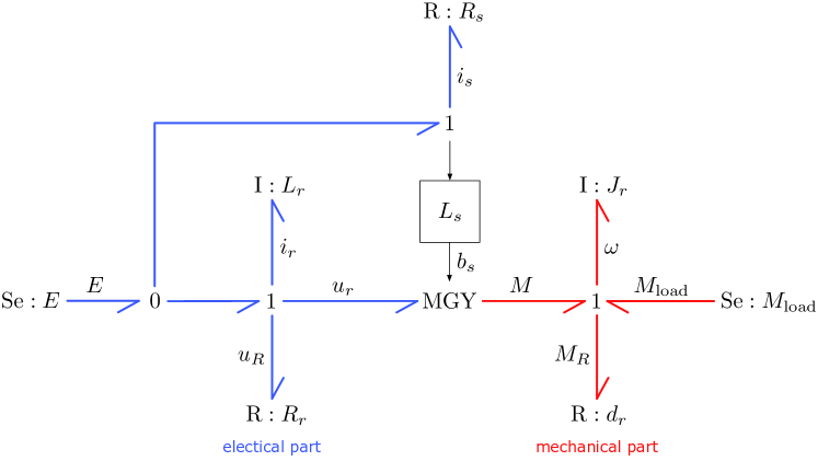
Figure 10: Bond graph model of a DC shunt motor.

We start with the bond graph model that is taken from [22] and redrawn in Figure 10. The half arrows are called bonds and each bond has two associated variables, called flow and effort. The name of the flow variable is written on the side of the arrow head, while the name of the effort variable is written on the opposite side. However, not all variables are explicitly named in the example. At any $0$-junction the effort variables of all connected bonds are equal, while the flow variables balance, with their sign given by the bond direction. Dually, at $1$-junctions flows are equal and efforts balance. Specifically, at the $0$-junction on the left the current from the $\mathrm{Se}$-element (effort source) with effort/voltage $E$ splits into the current $i_{s}$ through the stator coil and the current $i_{r}$ through the rotor coil. The inductance of the rotor coil is represented by the $\mathrm{I}$-element (generalized inductor) with inductance $L_{r}$, while an $\mathrm{I}$-element representing the stator coil inductance is omitted. The (steady-state) stator coil current $i_{s}$ is instead entirely determined by the $\mathrm{R}$-element (generalized resistor) at the top representing the coil’s electrical resistance $R_{s}$. The magnetic flux of the stator coil $b_{s}$ is instead obtained as the signal that results from multiplying the signal $i_{s}$, which is the shared effort variable at the upper $1$-junction, with the constant gain $L_{s}$. The bond graph hence combines energy-based modeling with signal-based modeling known from block diagrams. At the $1$-junction on the left, the source voltage $E$ is equal to the sum of the voltage over the rotor coil inductance $L_{r}$, the voltage $u_{R}$ over the rotor coil resistance $R_{r}$, and the induced (back EMF) voltage $u_{r}$. The latter is determined by the $\mathrm{MGY}$-element (modulated gyrator), which describes the coupling of the electrical and the mechanical parts. The gyrator ratio is the signal $b_{s}$ coming from the gain block. At the gyrator, the effort variable of one port is equal to the product of the gyrator ratio and the flow variable of the other port. On the mechanical side, the load torque $M_{\text{load}}\leq 0$ is modeled by the effort source on the right, while the rotor’s angular mass $J_{r}$ is represented by an $\mathrm{I}$-element. At the $1$-junction the sum of the generated torque $M$ and the load torque $M_{\text{load}}$ is equal to the sum of the torque accelerating the angular mass and the friction torque $M_{R}$. The latter is the product of the friction coefficient $d_{r}$ and the angular velocity $\omega$. Putting all this together, the bond graph gives the system of ordinary differential equations

$$L_{r}\,\derivative{i_{r}}{t}\> =\>E-u_{r}-u_{R}$$

$$J_{r}\,\derivative{\omega}{t}\> =\>M-M_{R}+M_{\text{load}}\,,$$

where

$$i_{s}\> =\>\frac{1}{R_{s}}\,E$$

$$b_{s}\> =\>L_{s}\,i_{s}$$

$$u_{r}\> =\>b_{s}\,\omega$$

$$M\> =\>b_{s}\,i_{r}$$

$$M_{R}\> =\>d_{r}\,\omega$$

$$u_{R}\> =\>R_{r}\,i_{r}\,.$$

As already shown in 4.3, the EPHS model is specified as an interconnection of two subsystems named $\mathtt{stator}$ and $\mathtt{rotor}$. The two systems share an electric energy domain represented by the junction with connected ports named $\mathtt{q}$. The kinetic energy domain of the rotor is represented by the junction with connected ports named $\mathtt{p}$. Both energy domains are exposed such that the motor model can be integrated into another system. The conversion between electric and kinetic energy in the rotor depends on the state of the magnetic energy domain of the stator, which is represented by the junction with connected state ports named $\mathtt{b_{s}}$.

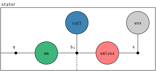
Figure 11: Interconnection pattern of the stator model.

The interconnection pattern of the stator model is shown in Figure 11. The box $\mathtt{em}$ is filled by a reversible component that represents the coupling of the electric energy domain with port $\mathtt{q}$ and the magnetic energy domain with port $\mathtt{b_{s}}$. The box $\mathtt{coil}$ is filled by a storage component that represents the inductance of the stator coil, while the box $\mathtt{emloss}$ is filled by an irreversible component that represents its electric resistance. The box $\mathtt{env}$ is filled by an environment component whose thermal energy domain with port $\mathtt{s}$ absorbs the dissipated electromagnetic energy.

The reversible component $(I_{\text{em}},\,\mathcal{D}_{\text{em}})$ is defined by its interface $I_{\text{em}}=(\{\mathtt{q},\,\mathtt{b_{s}}\},\,\tau_{\text{em}})$ with $\tau_{\text{em}}(\mathtt{q})=((\mathbb{R},\,\mathtt{charge}),\,\mathsf{p})$, $\tau_{\text{em}}(\mathtt{b_{s}})=((\mathbb{R},\,\mathtt{flux\_linkage}),\,\mathsf{p})$ and its Dirac structure $\mathcal{D}_{\text{em}}\subset\mathcal{P}_{I_{\text{em}}}$ given by

$$\begin{bmatrix}\mathtt{q.f}\\ \mathtt{b_{s}.f}\end{bmatrix}\>=\>\begin{bmatrix}0&1\\ -1&0\end{bmatrix}\,\begin{bmatrix}\mathtt{q.e}\\ \mathtt{b_{s}.e}\end{bmatrix}\,.$$

The storage component $(I_{\text{coil}},\,E_{\text{coil}})$ is defined by its interface $I_{\text{coil}}=(\{\mathtt{b_{s}}\},\,\tau_{\text{coil}})$ with $\tau_{\text{coil}}(\mathtt{b_{s}})=((\mathbb{R},\,\mathtt{flux\_linkage}),\,\mathsf{p})$ and its energy function $E_{\text{coil}}:\mathcal{X}_{I_{\text{coil}}}\rightarrow\mathbb{R}$ with $\mathcal{X}_{I_{\mathtt{coil}}}=\mathbb{R}\ni\mathtt{b_{s}.x}=b_{s}$ given by

$$E_{\mathtt{coil}}(b_{s})\>=\>\frac{1}{2\,L_{s}}\,b_{s}^{2}\,,$$

where the parameter $L_{s}$ is the inductance. Since $H_{\mathtt{coil}}=E_{\mathtt{coil}}$, the effort variable $\mathtt{b_{s}.e}=\frac{b_{s}}{L_{s}}$ is the current through the coil.

The irreversible component $(I_{\text{emloss}},\,\mathcal{O}_{\text{emloss}})$ is defined by $I_{\text{emloss}}=(\{\mathtt{b_{s}},\,\mathtt{s}\},\,\tau_{\text{emloss}})$ with $\tau_{\text{emloss}}(\mathtt{b_{s}})=((\mathbb{R},\,\mathtt{flux\_linkage}),\,\mathsf{p})$, $\tau_{\text{emloss}}(\mathtt{s})=((\mathbb{R},\,\mathtt{entropy}),\,\mathsf{p})$ and its Onsager structure $\mathcal{O}_{\text{emloss}}\subset\mathcal{P}_{\text{emloss}}$ given by

$$\begin{bmatrix}\mathtt{b_{s}.f}\\ \mathtt{s.f}\end{bmatrix}\>=\>\frac{1}{\color[rgb]{.5,0,.5}\theta_{0}}\,R_{s}\,\begin{bmatrix}{\color[rgb]{.5,0,.5}\theta_{0}+}\mathtt{s.e}&-\mathtt{b_{s}.e}\\ -\mathtt{b_{s}.e}&\frac{{(\mathtt{b_{s}.e})}^{2}}{{\color[rgb]{.5,0,.5}\theta_{0}+}\mathtt{s.e}}\end{bmatrix}\,\begin{bmatrix}\mathtt{b_{s}.e}\\ \mathtt{s.e}\end{bmatrix}\>=\>\begin{bmatrix}R_{s}\,\mathtt{b_{s}.e}\\ -\frac{R_{s}\,{(\mathtt{b_{s}.e})}^{2}}{{\color[rgb]{.5,0,.5}\theta_{0}+}\mathtt{s.e}}\end{bmatrix}\,,$$

where the parameter $R_{s}$ is the electric resistance of the coil.

The environment component is defined by the subinterface $I_{\text{env}}=\{\mathtt{s}\}\subseteq I_{R}$.

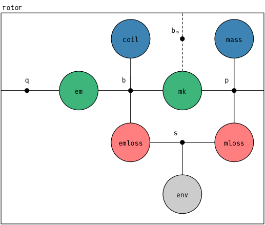
Figure 12: Interconnection pattern of the rotor model.

The interconnection pattern of the rotor model is shown in Figure 12. The components filling the boxes $\mathtt{coil}$, $\mathtt{em}$, $\mathtt{emloss}$, and $\mathtt{env}$ are defined as for the stator model, except for a different port name, namely $\mathtt{b}$ instead of $\mathtt{b_{s}}$, and different parameters, namely $L_{r}$ instead of $L_{s}$ and $R_{r}$ instead of $R_{s}$. The box $\mathtt{mk}$ is filled by a reversible component that describes the coupling of the magnetic energy domain with port $\mathtt{b}$ and the (rotational) kinetic energy domain with port $\mathtt{p}$. This coupling depends on the magnetic flux $\mathtt{b_{s}.x}$ that is generated by the stator coil. The box $\mathtt{mass}$ is filled by a storage component that represents the rotor’s angular mass and the box $\mathtt{mloss}$ is filled by an irreversible component that represents its mechanical friction.

The reversible component $(I_{\text{mk}},\mathcal{D}_{\text{mk}})$ is defined by $I_{\text{mk}}=(\{\mathtt{b},\,\mathtt{p},\,\mathtt{b_{s}}\},\,\tau_{\text{mk}})$ with $\tau_{\text{mk}}(\mathtt{b})=((\mathbb{R},\,\mathtt{flux\_linkage}),\,\mathsf{p})$, $\tau_{\text{mk}}(\mathtt{p})=((\mathbb{R},\,\mathtt{angular\_momentum}),\,\mathsf{p})$, $\tau_{\text{mk}}(\mathtt{b_{s}})=((\mathbb{R},\,\mathtt{flux\_linkage}),\,\mathsf{s})$ and its Dirac structure $\mathcal{D}_{\mathtt{mk}}\subset\mathcal{P}_{I_{\text{mk}}}$ given by

$$\begin{bmatrix}\mathtt{b.f}\\ \mathtt{p.f}\end{bmatrix}\>=\>\begin{bmatrix}0&\mathtt{b_{s}.x}\\ -\mathtt{b_{s}.x}&0\end{bmatrix}\,\begin{bmatrix}\mathtt{b.e}\\ \mathtt{p.e}\end{bmatrix}\,.$$

The storage component $(I_{\text{mass}},\,E_{\text{mass}})$ is defined by $I_{\text{mass}}=(\{\mathtt{p}\},\,\tau_{\text{mass}})$ with $\tau_{\text{mass}}(\mathtt{p})=((\mathbb{R},\,\mathtt{angular\_momentum}),\,\mathsf{p})$ and $E_{\text{mass}}:\mathcal{X}_{I_{\text{mass}}}\rightarrow\mathbb{R}$ with $\mathcal{X}_{I_{\text{mass}}}=\mathbb{R}\ni\mathtt{p.x}=p$ given by

$$E_{\text{mass}}(p)\>=\>\frac{1}{2\,J_{r}}\,p^{2}\,,$$

where the parameter $J_{r}$ is the angular mass.

The irreversible component $(I_{\text{mloss}},\mathcal{O}_{\text{mloss}})$ is defined by $I_{\text{mloss}}=(\{\mathtt{p},\,\mathtt{s}\},\,\tau_{\text{mloss}})$ with $\tau_{\text{mloss}}(\mathtt{p})=((\mathbb{R},\,\mathtt{angular\_momentum}),\,\mathsf{p})$, $\tau_{\text{mloss}}(\mathtt{s})=((\mathbb{R},\,\mathtt{entropy}),\,\mathsf{p})$ and its Onsager structure $\mathcal{O}_{\text{mloss}}\subset\mathcal{P}_{I_{\text{mloss}}}$ given by

$$\begin{bmatrix}\mathtt{p.f}\\ \mathtt{s.f}\end{bmatrix}\>=\>\frac{1}{\color[rgb]{.5,0,.5}\theta_{0}}\,d_{r}\,\begin{bmatrix}{\color[rgb]{.5,0,.5}\theta_{0}+}\mathtt{s.e}&-\mathtt{p.e}\\ -\mathtt{p.e}&\frac{{(\mathtt{p.e})}^{2}}{{\color[rgb]{.5,0,.5}\theta_{0}+}\mathtt{s.e}}\end{bmatrix}\,\begin{bmatrix}\mathtt{p.e}\\ \mathtt{s.e}\end{bmatrix}\>=\>\begin{bmatrix}d_{r}\,\mathtt{p.e}\\ -\frac{d_{r}\,{(\mathtt{p.e})}^{2}}{{\color[rgb]{.5,0,.5}\theta_{0}+}\mathtt{s.e}}\end{bmatrix}\,,$$

where the parameter $d_{r}$ is the mechanical friction coefficient.

We write $(b_{s},\,b,\,p,\,s)\in\mathbb{R}^{4}$ for the state of the interconnected motor model, where we identify the entropy state variables $s$ of both environment components. In future work, the identification of environment components can be formalized by composing with a suitable relation. The EPHS model then yields the equations

$$\dot{b}_{s}\> =\>\mathtt{q.e}-R_{s}\,i_{s}$$

$$\dot{b}\> =\>\mathtt{q.e}-b_{s}\,\omega-R_{r}\,i_{r}$$

$$\dot{p}\> =\>b_{s}\,i_{r}-d_{r}\,\omega+\mathtt{p.f}$$

$$\dot{s}\> =\>\frac{1}{{\color[rgb]{.5,0,.5}\theta_{0}}}\left(R_{s}\,i_{s}^{2}+R_{r}\,i_{r}^{2}+d_{r}\,\omega^{2}\right)$$

$$\mathtt{q.f}\> =\>i_{s}+i_{r}\,,$$

where

$$i_{s}\> =\>\frac{1}{L_{s}}\,b_{s}$$

$$i_{r}\> =\>\frac{1}{L_{r}}\,b$$

$$\omega\> =\>\frac{1}{J_{r}}\,p\,.$$

10 Discussion

While it still seems reasonable to package a motor model as a single bond graph, integrating the model as part of a more complex system is not supported by the bond graph notation. Hence, bond graph users have to reproduce models as parts of more complex models. EPHS improves upon this, making it nearly trivial to encapsulate, reuse, and swap out submodels. Another main feature of EPHS is their built-in thermodynamic consistency. Restricting the space of models in this way not only provides important guarantees, it also makes models compatible with each other, as a close link between their mathematical structure and physical interpretation is established. This is reflected by the correspondence of junctions and energy domains, which in our opinion contributes substantially to the improved readability of the EPHS syntax. The reason why EPHS users can easily integrate existing models without first needing to adapt them to fit into the larger system is that EPHS simply compose by sharing energy domains. In this way, we hope to improve upon port-Hamiltonian systems, which lack an intuitive graphical syntax and require that users define the ports of a system in a somewhat arbitrary manner.

Author contribution statement

Markus Lohmayer: Conceptualization, Investigation, Writing – Original Draft, Writing – Review & Editing, Visualization; Owen Lynch: Investigation, Writing – Original Draft; Sigrid Leyendecker: Supervision

References

- Courant [1990] T. J. Courant, Dirac manifolds, Transactions of the American Mathematical Society 319 (1990) 631–661.
- Pavelka et al. [2018] M. Pavelka, V. Klika, M. Grmela, Multiscale Thermo-Dynamics, De Gruyter, Berlin, 2018. doi:10.1515/9783110350951.
- Callen [1985] H. Callen, Thermodynamics and an Introduction to Thermostatistics, second ed., John Wiley & Sons Inc, New York, 1985.
- Öttinger [2005] H. C. Öttinger, Beyond Equilibrium Thermodynamics, John Wiley & Sons Inc, Hoboken, New Jersey, 2005.
- de Groot and Mazur [1984] S. de Groot, P. Mazur, Non-equilibrium Thermodynamics, Dover Books on Physics, Dover Publications, New York, 1984.
- Onsager [1931] L. Onsager, Reciprocal relations in irreversible processes. i., Physical Review 37 (1931) 405–426.
- Breedveld [1982] P. C. Breedveld, Thermodynamic bond graphs and the problem of thermal inertance, Journal of the Franklin Institute 314 (1982) 15 – 40.
- Maschke [1991] B. Maschke, Geometrical formulation of bond graph dynamics with application to mechanisms, Journal of the Franklin Institute 328 (1991) 723–740.
- Willems [1974] J. C. Willems, Qualitative behavior of interconnected systems, in: Annals of Systems Research, Springer US, 1974, pp. 61–80. doi:10.1007/978-1-4613-4555-8_4.
- Willems [2007] J. C. Willems, The behavioral approach to open and interconnected systems, IEEE Control Systems 27 (2007) 46–99.
- Maschke et al. [1992] B. Maschke, A. van der Schaft, P. Breedveld, An Intrinsic Hamiltonian Formulation of Network Dynamics: Non-standard Poisson Structures and Gyrators, Journal of the Franklin Institute 329 (1992) 923–966.
- van der Schaft and Maschke [1995] A. van der Schaft, B. Maschke, The Hamiltonian formulation of energy conserving physical systems with external ports, AEU - Archiv für Elektronik und Übertragungstechnik 49 (1995) 362–371.
- van der Schaft and Jeltsema [2014] A. van der Schaft, D. Jeltsema, Port-Hamiltonian systems theory: An introductory overview, Foundations and Trends in Systems and Control 1 (2014) 173–378.
- Grmela and Öttinger [1997] M. Grmela, H. C. Öttinger, Dynamics and thermodynamics of complex fluids. I. Development of a general formalism, Phys. Rev. E 56 (1997) 6620–6632.
- Kaufman [1984] A. N. Kaufman, Dissipative Hamiltonian systems: A unifying principle, Physics Letters A 100 (1984) 419–422.
- Grmela [1984a] M. Grmela, Particle and bracket formulations of kinetic equations, in: Fluids and plasmas: geometry and dynamics (Boulder, Colo., 1983), volume 28 of Contemp. Math., Amer. Math. Soc., Providence, RI, 1984a, pp. 125–132. doi:10.1090/conm/028/751978.
- Grmela [1984b] M. Grmela, Bracket formulation of dissipative fluid mechanics equations, Physics Letters A 102 (1984b) 355–358.
- Morrison [1984] P. J. Morrison, Bracket formulation for irreversible classical fields, Physics Letters A 100 (1984) 423–427.
- Badlyan et al. [2018] A. M. Badlyan, B. Maschke, C. Beattie, V. Mehrmann, Open physical systems: from GENERIC to port-Hamiltonian systems, in: Proceedings of the 23rd International Symposium on Mathematical Theory of Systems and Networks, Hong Kong, China, 2018, pp. 204–211.
- Lohmayer et al. [2021] M. Lohmayer, P. Kotyczka, S. Leyendecker, Exergetic port-Hamiltonian systems: modelling basics, Mathematical and Computer Modelling of Dynamical Systems 27 (2021) 489–521.
- Paynter [1961] H. Paynter, Analysis and Design of Engineering Systems, MIT Press, Cambridge, 1961.
- Borutzky [2010] W. Borutzky, Bond Graph Methodology, Springer London, 2010. doi:10.1007/978-1-84882-882-7.
- Birkett and Roe [1989] S. Birkett, P. Roe, The mathematical foundations of bond graphs—i. algebraic theory, Journal of the Franklin Institute 326 (1989) 329–350.
- Coya [2017] B. Coya, A compositional framework for bond graphs, 2017. doi:10.48550/ARXIV.1710.00098.
- Pfeifer et al. [2020] M. Pfeifer, S. Caspart, S. Hampel, C. Muller, S. Krebs, S. Hohmann, Explicit port-Hamiltonian formulation of multi-bond graphs for an automated model generation, Automatica 120 (2020) 109121.
- Mac Lane [1998] S. Mac Lane, Categories for the Working Mathematician, Graduate Texts in Mathematics, second ed., Springer, 1998.
- Fong and Spivak [2019] B. Fong, D. I. Spivak, An Invitation to Applied Category Theory, Cambridge University Press, 2019. doi:10.1017/9781108668804.
- Myers [2022] D. J. Myers, Categorical systems theory, http://davidjaz.com/Papers/DynamicalBook.pdf, 2022.
- Baez and Erberle [2015] J. Baez, J. Erberle, Categories in control, Theory and Applications of Categories 30 (2015) 836–881.
- Baez and Pollard [2017] J. C. Baez, B. S. Pollard, A compositional framework for reaction networks, Reviews in Mathematical Physics 29 (2017) 1750028.
- Baez and Fong [2018] J. C. Baez, B. Fong, A compositional framework for passive linear networks, 2018. doi:10.48550/ARXIV.1504.05625.
- Baez et al. [2020] J. C. Baez, J. Foley, J. Moeller, B. S. Pollard, Network models, 2020.
- Foley et al. [2021] J. D. Foley, S. Breiner, E. Subrahmanian, J. M. Dusel, Operads for complex system design specification, analysis and synthesis, Proceedings of the Royal Society A: Mathematical, Physical and Engineering Sciences 477 (2021) 20210099.
- Leinster [2004] T. Leinster, Higher Operads, Higher Categories, London Mathematical Society Lecture Note Series, Cambridge University Press, 2004. doi:10.1017/CBO9780511525896.
- Yau [2016] D. Yau, Colored Operads, American Mathematical Society (AMS), Providence, Rhode Island, 2016.
- Lohmayer and Leyendecker [2022] M. Lohmayer, S. Leyendecker, EPHS: A Port-Hamiltonian Modelling Language, in: 25th IFAC Symposium on Mathematical Theory of Networks and Systems MTNS 2022, volume 55, Elsevier BV, 2022, pp. 347–352. doi:10.1016/j.ifacol.2022.11.077.
- Spivak [2013] D. I. Spivak, The operad of wiring diagrams: formalizing a graphical language for databases, recursion, and plug-and-play circuits, 2013. doi:10.48550/ARXIV.1305.0297.
- Spivak [2014] D. Spivak, Category Theory for the Sciences, MIT Press, 2014.
- Yau [2018] D. Yau, Operads of Wiring Diagrams, Springer International Publishing, 2018. doi:10.1007/978-3-319-95001-3.
- Breiner et al. [2020] S. Breiner, B. Pollard, E. Subrahmanian, O. Marie-Rose, Modeling hierarchical system with operads, Electronic Proceedings in Theoretical Computer Science 323 (2020) 72–83.
- Vagner et al. [2015] D. Vagner, D. Spivak, E. Lerman, Algebras of open dynamical systems on the operad of wiring diagrams, Theory and Applications of Categories 30 (2015) 1793–1822.
- Schultz et al. [2019] P. Schultz, D. I. Spivak, C. Vasilakopoulou, Dynamical systems and sheaves, Applied Categorical Structures 28 (2019) 1–57.
- Libkind [2020] S. Libkind, An algebra of resource sharing machines, 2020. doi:10.48550/ARXIV.2007.14442.
- Libkind et al. [2021] S. Libkind, A. Baas, E. Patterson, J. Fairbanks, Operadic modeling of dynamical systems: Mathematics and computation, 2021. doi:10.48550/ARXIV.2105.12282.
- Lynch [2022] O. Lynch, Relational composition of physical systems: A categorical approach, 2022. doi:10.48550/arXiv.2310.06088.
- Fredkin [1960] E. Fredkin, Trie memory, Communications of the ACM 3 (1960) 490–499.
- Pavelka et al. [2014] M. Pavelka, V. Klika, M. Grmela, Time reversal in nonequilibrium thermodynamics, Phys. Rev. E 90 (2014) 062131.
- Lee [2012] J. M. Lee, Introduction to Smooth Manifolds, second ed., Springer New York, 2012. doi:10.1007/978-1-4419-9982-5.
- Bursztyn [2013] H. Bursztyn, A brief introduction to Dirac manifolds, in: A. Cardona, I. Contreras, A. F. Reyes-Lega (Eds.), Geometric and Topological Methods for Quantum Field Theory: Proceedings of the 2009 Villa de Leyva Summer School, Cambridge University Press, Cambridge, 2013, p. 4–38. doi:10.1017/CBO9781139208642.002.
- Mielke et al. [2016] A. Mielke, D. R. M. Renger, M. A. Peletier, A generalization of Onsager’s reciprocity relations to gradient flows with nonlinear mobility, Journal of Non-Equilibrium Thermodynamics 41 (2016).
- Willems [1972] J. C. Willems, Dissipative dynamical systems part I: General theory, Archive for Rational Mechanics and Analysis 45 (1972) 321–351.