Local heat current flow in the ballistic phonon transport of graphene nanoribbons

Abstract

Utilizing nonequilibrium Green’s function method, we study the phonon local heat current flow in nanoscale graphene nanoribbons. Ballistic transport and boundary scattering lead to formation of atomic scale current vortices. Using the Büttiker probe approach, we further map out the temperature distribution in the junction. From the heat current and temperature distribution, we observe negative local resistance of the junctions, where heat current direction goes from colder to hotter regime. Moreover, we show that atomic scale defect can generate heat vortex at certain frequency, but it is averaged out when including contributions from all the phonon modes. These results extend the study of local heat vortex and negative temperature response in bulk hydrodynamic regime to atomic-scale ballistic regime, further confirming boundary scattering is crucial to generate backflow of heat current.

I Introduction

Quantum transport properties of nanoscale systems have received intense attention in the past several decades. Single molecular junction is one example of such systems, enabling the study of fundamental physical phenomena at atomic level, especially the out-of-equilibrium transport properties of heat and charge[1, 2, 3, 4]. For electronic transport, while most of the works focused on the global transport properties, some efforts were made to unveil local contribution of electron charge current within molecular junctions [5, 6, 7, 8, 9, 10, 11, 12, 13]. The investigation of local current provides insight into the detailed behavior of electrons in the molecular junction, such as quantum interference and vortex dynamics [7, 9, 10, 13].

In larger two-dimensional (2D) atomic structures, local currents are calculated to achieve quantitative understanding of transport mechanisms and support the design of effective nanoscale devices [14, 15, 16, 17, 18, 19, 20, 21, 22, 23, 24, 25, 26, 27, 28, 29, 30, 31, 32, 33]. Recently, electron current vortices have been explored intensively as a signature of hydrodynamic transport in 2D systems [34, 35], which induces negative non-local electrical resistance [36, 37, 38, 39, 40]. Later, these novel transport behaviors have also been predicted to appear in ballistic transport regime [27, 31].

On the other hand, thermal transport in 2D materials has also received intense research interest[41, 42]. Theoretical works demonstrated that phonon heat vortices can exist in both hydrodynamic and ballistic regimes [43, 44, 45, 46, 47]. Motivated by the intriguing thermal features provided in previous works, we extend these ideas to nanoscale atomic structures, where wave property of phonons becomes important. We study the local heat current and temperature distribution in graphene nanoribbons, paying special attention to the effects of boundary scattering and atomic defect [48, 49].

We use the nonequilibrium Green’s function (NEGF) method to describe coherent phonon transport[50]. Specifically, we derive the expression for the local heat current, calculate heat flow in real space and further study the emerging heat vortices. Different from electronic transport where the current is mainly contributed by electrons near the Fermi level, the phonon heat current includes contribution from all the phonon modes. Thus, the emergence of heat vortices is not obvious. We analyze how the vortices depend on the geometric factors of the ribbon, the way heat is injected and extracted from the system, and how they are influenced by atomic disorder. Then, by calculating the local heat current in the ribbon with defects, we compare the results obtained by earlier studies that suggested the formation of vortices by specific local defect states [51, 52].

In addition to the heat flow, we also study the local temperature distribution, which is of great interest in nonequilibrium thermodynamics. The local temperature can be defined in various ways [53]. In classical simulations, it is defined using the kinetic energy of atomic degrees of freedom from the equipartition theorem [54, 55]. Analogous to thermometers, Büttiker probe and self-consistent reservoir have been used to determine local temperature when they reach local equilibrium with the system of interest [56, 57, 58, 59, 60, 61, 62, 63, 64, 65, 66]. The statistical definition for temperature [67, 68] and fluctuation-dissipation theorem [69, 70, 71] have also been generalized to express local temperature. Although these definitions give consistent results at equilibrium, they do not necessarily coincide with each other in nonequilibrium systems. In terms of experiments, local temperature can be measured in tens-of-nanometer-scale resolution using scanning thermal microscopy technique [72]. This setup is similar to the idea of Büttiker probe, which we use here [65].

II Theory

II.1 Local heat current in harmonic system

We start with a Hamiltonian $H$ within the harmonic approximation:

$$H=\sum_{n,i}\left(\frac{1}{2}\dot{u}_{ni}^{2}+\sum_{m,j}\frac{1}{2}u_{ni}K_{ni,mj}u_{mj}\right).$$ (1)

Here we use the mass-normalized displacements $u_{ni}=\sqrt{m_{n}}x_{ni}$, $x_{ni}$ is the displacement away from the equilibrium position of $n$-th atom along $i$ axis ($i,j=x,y,z$) and the indices run over all degrees of freedom in the system. The spring constant matrix has the symmetry $K_{ni,mj}=K_{mj,ni}$. In quantum regime, $u_{i}$ and $\dot{u}_{i}$ turn into operators, satisfying the commutation relation $[u_{ni},\dot{u}_{mj}]=i\hbar\delta_{nm}\delta_{ij}$. The system is divided into three parts: the central region with finite degrees of freedom driven out of equilibrium, the left ($L$) and right ($R$) reservoirs with infinite degrees of freedom and in equilibrium.

We then rewrite the total Hamiltonian as:

$$H=\sum_{\alpha=L,R}(H_{\alpha}+H_{\alpha C})+H_{C},$$ (2)

with

$$H_{\alpha} =\sum_{i,n\in\alpha}(\frac{1}{2}\dot{u}_{ni}^{2}+\sum_{j,m\in\alpha}\frac{1}{2}u_{ni}K_{ni,mj}^{\alpha}u_{mj}),$$ (3)

$$H_{C} =\sum_{i,n\in C}(\frac{1}{2}\dot{u}_{ni}^{2}+\sum_{j,m\in C}\frac{1}{2}u_{ni}K_{ni,mj}^{C}u_{mj}),$$ (4)

$$H_{\alpha C} =\sum_{\begin{subarray}{c}i,n\in C\\ j,m\in\alpha\end{subarray}}\frac{1}{2}(u_{ni}V_{ni,mj}u_{mj}+u_{mj}V_{mj,ni}u_{ni}),$$ (5)

where $C$ denotes the central region, and $V_{ni,mj}=V_{mj,ni}$ is the coupling matrix of the reservoir and the central region.

One can calculate heat current from reservoir $\alpha$ to the central region using standard NEGF method [73, 50, 74, 75, 76]. Meanwhile, the local heat current $J_{nm}$ from atom site $n$ to site $m$ in the central region can be defined intuitively from the continuity equation

$$\partial_{t}h_{n}+\sum_{m(\neq n)}J_{nm}=0,$$ (6)

where $h_{n}$ is the local energy. In this work, we choose $h_{n}$ containing kinetic energy terms of atom $n$, all coupling terms with reservoirs, and half of the harmonic terms between atom sites:

$$\begin{split}h_{n}&=\sum_{i}\frac{1}{2}\Big{[}\dot{u}_{ni}^{2}+\sum_{j,m\in C}u_{ni}K_{ni,mj}^{C}u_{mj}\\ &\quad+\sum_{j,m\in\alpha}(u_{ni}V_{ni,mj}u_{mj}+u_{mj}V_{mj,ni}u_{ni})\Big{]}.\end{split}$$ (7)

Now, the decomposition of the total Hamiltonian becomes $H=\sum_{\alpha}H_{\alpha}+\sum_{n\in C}h_{n}$, similar definitions were used in other works [77, 78, 79, 80, 81, 82, 83, 84, 85, 86, 87]. Then, from the Heisenberg equation of motion, we get

$$\begin{split}-\frac{\partial h_{n}}{\partial t}&=\frac{i}{\hbar}[h_{n},H]\\ &=\frac{1}{2}\sum_{i,j,m\in C}(u_{mj}K_{mj,ni}^{C}\dot{u}_{ni}-u_{ni}K_{ni,mj}^{C}\dot{u}_{mj})\\ &\quad-\frac{1}{2}\sum_{i,j,m\in\alpha}(u_{ni}V_{ni,mj}\dot{u}_{mj}+\dot{u}_{mj}V_{mj,ni}u_{ni}).\end{split}$$ (8)

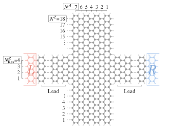
Figure 1: A sketch of the two terminal graphene nanoribbon. The reservoirs ($L$ and $R$) are connected to the ribbon through narrower leads, such that heat can be locally injected or extracted from the ribbon. $N^{Z}$, $N^{Z}_{\rm Res}$ and $N^{A}$ are geometric parameters.

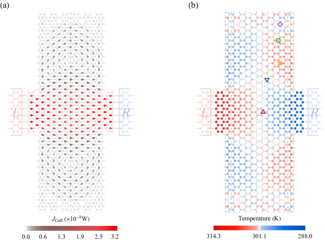
Figure 2: Spatial pattern of local heat current (a) and local temperature (b) for a temperature bias of $T_{L}=325$ K, $T_{R}=275$ K. The coupling strength of the system and the temperature probe is $\hbar\gamma_{p}=0.065$ meV. Geometric parameters: $N^{Z}=30$, $N^{A}=11$ and $N^{Z}_{\rm Res}=6$.

Here, the first term after the second equal sign represents the local heat current flowing out of site $n$, the second term equals to the heat current $J_{\alpha}$ from reservoir $\alpha$ in steady state. The definition of local energy in Eq. (7) is not unique [88, 89, 90, 91], however, the degrees of freedom selected for $h_{n}$ are simply different views (or resolutions) to study the nanosystem, having no effect on the energy flow in the harmonic quantum network since phonon dynamics is established as the Hamiltonian is defined. Rewrite the formula for local heat current in the form of Green’s functions [92, 93, 51, 94, 95, 96, 97, 98, 99, 100], we have

$$\begin{split}J_{nm}=\frac{i\hbar}{2}\frac{\partial}{\partial t}&\sum_{i,j}\Big{[}K_{mj,ni}^{C}G^{<}_{ni,mj}(t,t^{\prime})\\ &\qquad-K_{ni,mj}^{C}G^{<}_{mj,ni}(t,t^{\prime})\Big{]}|_{t^{\prime}\to t},\end{split}$$ (9)

where $i\hbar G^{<}_{ni,mj}(t,t^{\prime})=\langle u_{mj}(t^{\prime})u_{ni}(t)\rangle$ is the lesser Green’s function, and the greater Green’s function $i\hbar G^{>}_{ni,mj}(t,t^{\prime})=\langle u_{ni}(t)u_{mj}(t^{\prime})\rangle$ can be defined accordingly. In steady state, it is convenient to work in the frequency domain, the lesser Green’s function satisfies the following equation [101], which is expressed in terms of the retarded Green’s function $\bm{G}^{r}(\omega)$, the advanced Green’s function $\bm{G}^{a}(\omega)$, and the lesser self-energy $\bm{\Sigma}^{<}(\omega)$ in matrix form:

$$\bm{G}^{<}(\omega) =\bm{G}^{r}(\omega)\bm{\Sigma}^{<}(\omega)\bm{G}^{a}(\omega),$$ (10)

$$\bm{G}^{r}(\omega) =[(\omega+i\eta)^{2}-\bm{K}^{C}-\bm{\Sigma}^{r}(\omega)]^{-1},$$ (11)

$$\bm{G}^{a}(\omega) =[\bm{G}^{r}(\omega)]^{\dagger}.$$ (12)

Here, $\bm{\Sigma}^{<,r,a}(\omega)=\sum_{\alpha}\bm{\Sigma}^{<,r,a}_{\alpha}(\omega)$ are the lesser, retarded and advanced self-energies due to the coupling to the reservoirs. Introducing the Bose-Einstein distribution function $f_{\alpha}(\omega)=[e^{(\hbar\omega/k_{B}T_{\alpha})}-1]^{-1}$ for reservoir $\alpha$ with temperature $T_{\alpha}$, we have

$$\bm{\Sigma}^{<}_{\alpha}(\omega) =-if_{\alpha}(\omega)\bm{\Gamma}_{\alpha}(\omega),$$ (13)

$$\bm{\Sigma}^{>}_{\alpha}(\omega) =-i(1+f_{\alpha}(\omega))\bm{\Gamma}_{\alpha}(\omega).$$ (14)

with $\bm{\Gamma}_{\alpha}(\omega)=i[\bm{\Sigma}^{r}_{\alpha}(\omega)-\bm{\Sigma}^{a}_{\alpha}(\omega)]$. Substituting Eqs. (10-14) into Eq. (9), we obtain a Landauer-like expression for the local heat current (see details in Appendix A):

$$J_{nm}=\sum_{\alpha(\neq\beta)}\int^{+\infty}_{0}\frac{d\omega}{2\pi}\hbar\omega\mathcal{T}^{\beta\alpha}_{nm}(\omega)[f_{\beta}(\omega)-f_{\alpha}(\omega)],$$ (15)

with

$$\begin{split}\mathcal{T}^{\beta\alpha}_{nm}(\omega)&=-\sum_{i,j}\Big{\{}K_{mj,ni}^{C}\text{Im}[\bm{G}^{r}\bm{\Gamma}_{\alpha}\bm{G}^{a}]_{ni,mj}(\omega)\\ &-K_{ni,mj}^{C}\text{Im}[\bm{G}^{r}\bm{\Gamma}_{\alpha}\bm{G}^{a}]_{mj,ni}(\omega)\Big{\}}\quad(\alpha\neq\beta).\end{split}$$ (16)

The current expression here is summed over all polarization directions of site $m$ and $n$.

II.2 Local Temperature

For a unique and practical definition of temperatures, an approach inspired by the zeroth law of thermodynamics have been developed [102, 71, 103, 104, 64, 65]. Wherein, an extra reservoir coupled locally to the system is introduced as a temperature probe that the local temperature is obtained by vanishing net heat current between the probe and the system. Here we take the subscript $p$ for the temperature probe. This can be expressed as:

$$J_{p}=\sum_{\alpha}\int_{0}^{\infty}\frac{d\omega}{2\pi}\hbar\omega\mathcal{T}^{p\alpha}(\omega)[f_{p}(\omega)-f_{\alpha}(\omega)]=0,$$ (17)

where $\mathcal{T}^{p\alpha}(\omega)=$Tr$[\bm{G}^{r}\bm{\Gamma}_{p}\bm{G}^{a}\bm{\Gamma}_{\alpha}](\omega)$ is the transmission function between lead $\alpha$ and the temperature probe. It was shown in Refs. [64, 65] that for a wide-band and weakly coupled probe, there exists a unique solution for the local electron temperature and chemical potential. In this limit, density of states in the probe have no effect on the temperature and the local heat current is left unperturbed. The local temperature obtained with this method in nonequilibrium system is compatible with scanning thermal microscopic techniques, although some coarse-graining is needed due to the limited spatial resolution of the scanning probe.

As a theoretical analysis, the calculation of local temperature in this work is conducted by coupling only one atom to the probe at a time. The self-energy of the probe coupled to an atom can be written explicitly as $[\bm{\Sigma}_{p}^{r}(\omega)]_{ni,mj}=-i\gamma_{p}\omega\delta_{ij}\delta_{nm}\delta_{np}$, where the non-diagonal elements are taken to be zero and $\delta_{np}$ at the end suggests only the $n$-th atom coupled to the probe have nonzero elements. In Fig. 3(c), we verified that when $\hbar\gamma_{p}$ is far weaker than the system energy scale (the maximum energy of phonon dispersion in pristine graphene is $\sim 200$ meV), the local temperature sampled by the probe is independent of the system-probe coupling strength $\gamma_{p}$.

III Numerical results

III.1 Vortex formation due to local current injection

Consider a graphene nanoribbon connected to two reservoirs, we use parameters $N^{Z}$ and $N^{A}$ to represent the number of hexagon cell at zigzag and armchair edge respectively. The reservoirs are connected to the longer zigzag edge through armchair leads, as shown in Fig. 1. The geometric parameter for armchair leads and reservoirs is given by $N^{Z}_{\rm Res}$. Notice that the dimension of the nanoribbon is in nanometer scale, far smaller than the mean free path of phonon-phonon scattering in pristine graphene [105, 106]. In this case, ballistic transport dominates and phonons are scattered elastically.

In the following numerical calculation, the spring constant matrix is generated using LAMMPS [107], where the empirical bond order potential [108] is employed for C-C and C-H interaction and Tersoff’s potential [109] is used for Si-C interaction. The edges of the ribbon is passivated by Hydrogen atoms.

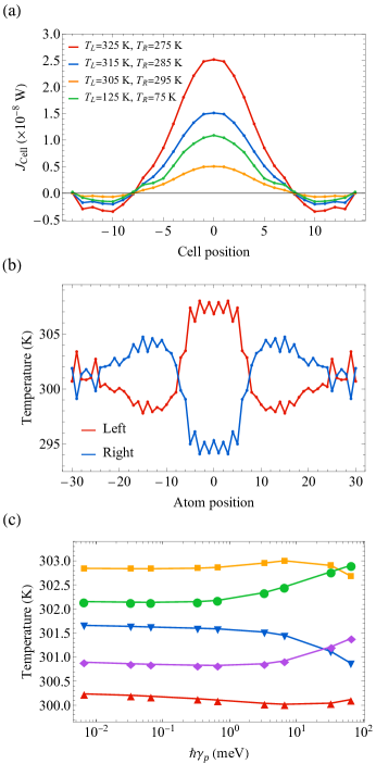
Figure 3: Detailed profile of Fig. 2. (a) Local heat flux across the vertical dashed line cut in Fig. 2(a). The cell position is counted from bottom to top along the line cut. (b) Local temperature extracted on the left and right border marked by dashed boxes in Fig. 2(b). (c) Local temperature of the atoms shown in Fig. 2(b) with same color markers as a function of the coupling parameter $\gamma_{p}$.

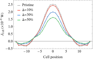
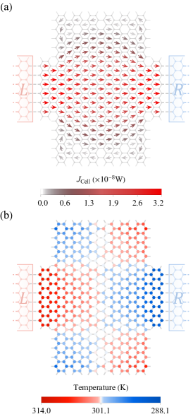
Figure 4: Local heat flux in the ribbon with mass disorder, where $\Delta$ is the disorder strength. The disordered current pattern is averaged from 50 ensembles. The rest of the parameters are the same in Fig. 2.

Figure 5: Thermal profile in a narrow ribbon. (a) Local heat current. (b) Local temperature. Geometric parameters: $N^{Z}=16$, $N^{Z}_{\rm Res}=6$ and $N^{A}=11$. The rest of the settings are the same as Fig. 2.

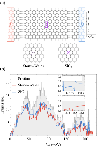
Figure 6: Zigzag graphene nanoribbon with defects. $N^{A}=9$ is the only parameter to mark its width. (a) A sketch of the ribbon and defects. The defect is placed at the middle marked by the purple box. (b) Transmission of zigzag graphene nanoribbon with Stone-Wales and $\mathrm{SiC_{4}}$ defects. Insets show phonon modes with zero transmission.

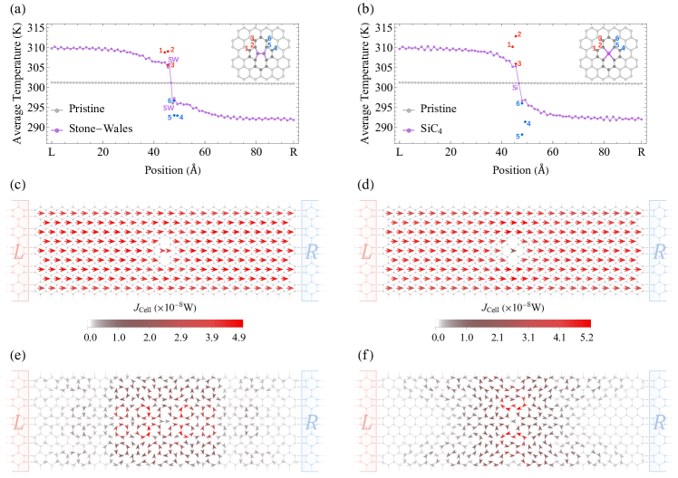
Figure 7: Local heat current and temperature of zigzag graphene nanoribbon with Stone-Wales (SW) (a, c, e) and $\mathrm{SiC_{4}}$ (b, d, f) defect. Local temperatures in (a) and (b) are averaged by the atoms sharing same horizontal coordinate, from the left reservoir to the right. The scattered points with number correspond to the atoms in the insets. (c-d) Local heat current through the defect atoms are given by $\vec{J}_{n}=\sum_{m(\neq n)}\vec{J}_{nm}$, the color gradient is consistent with $\vec{J}_{\rm Cell}$. (e-f) Frequency resolved $\vec{J}_{n}$ at $\hbar\omega=157.87$ (e) and $150.02$ meV (f). These frequencies are found in the insets of Fig. 6.

One example of the calculated local temperature and local heat current distribution is presented in Fig. 2, with the parameters given in the figure caption. The spatial distribution of local heat current is calculated using Eqs. (15) and (16). The arrows result from the sum of $\vec{J}_{nm}$ among six atoms in the corresponding hexagon cell $\vec{J}_{\rm Cell}=\sum_{\{n,m\}\in\rm Cell}\vec{J}_{nm}$. Color and orientation of the arrows mark the magnitude and direction of the local heat current. We can see that dominant contribution of the heat current from $L$ to $R$ comes from the region that directly connects the two leads (red region). Current vortices appear at both sides of this region (gray region), and they do not contribute to the total heat current. Comparing with the local temperature distribution, we find that the current does not always flow from hotter to colder region. There are regions with backflow current from colder to hotter region.

Detailed temperature profiles are depicted in Fig. 3. The current flowing through the dashed line cut in Fig. 2(a) is depicted in Fig. 3(a), the backflow current is at 10%$\sim$15% of the maximum in the ribbon, while the backflow current in bulk graphene system was reported two orders of magnitude smaller than mainstream flow in the middle[110, 47]. The results also indicate that the temperature bias of the reservoirs has little impact on the spatial pattern of local current. In Fig. 3(b), we extract the local temperature on the left and right border of the ribbon, marked by the dashed boxes in Fig. 2(b). The averaged temperature in the ribbon is approximated at 301K, slightly higher than the averaged temperature of the reservoirs ($300$K). The opposite temperature distribution is quite noticeable compare to the atoms subjected to the leads in the middle. In order to verify the proclaimed assumption in Sec. II.2, we check the sampled temperature by tuning the coupling strength $\gamma_{p}$. Results in Fig. 3(c) confirm that, in the weak coupling limit, local temperature obtained from the probe remains unaffected by the system-probe coupling.

In a realistic setup, disturbances are inevitable, leading to inhomogeneity in the graphene nanoribbon. Here, we consider mass-disorder to model elastic scattering [111, 112, 113, 114], such global disturbance is possible when the ribbon is attached to a substrate. Disorder in the ribbon is realized by randomly altering the mass of the atoms in spring constant $K^{C}$. Randomized mass $m_{n}^{\prime}$ for the $n$-th atom is chosen from a uniform distribution between $m_{n}(1-\Delta)$ and $m_{n}(1+\Delta)$, where $\Delta$ is the disorder strength. It can be seen in Fig. 5 that although the transmitting current decreases substantially with the increase of $\Delta$, the backflow heat current survive the disorder, even at $\Delta=50\%$. The backflow current near $\pm 10$th cells indicate slight distortion of vortex pattern by disorder. Similar result was mentioned by earlier study in electron system [31].

In ballistic regime, prior studies emphasized that phonons are scattered by the borders in pristine graphene nanoribbon[110, 46, 47]. Heat vortices are induced by reflection on the vertical borders opposite the injection leads. If the size of vertical borders are comparable to the horizontal ones, the current are more likely to be reflected by the horizontal borders on the top and bottom, which do not contribute to the backflow. One example with $N^{Z}=16$, $N^{Z}_{\rm Res}=6$ and $N^{A}=11$ is shown in Fig. 5. In such a confined system, only the middle mainstream persists. The spiraling whirlpools at the corner result from competitive scattering by vertical and horizontal borders. Although the net heat current flows directly from left to right, there still exists opposite temperature response in Fig. 5(b). Based on the trials conducted, we reach to the conclusion that noticeable backflow occurs when the geometric parameters satisfy a rough ratio: $N^{Z}-N^{Z}_{\rm Res}>N^{A}$. Furthermore, we have also checked the results in the ribbon with longer armchair edge ($N^{A}>N^{Z}$), where the leads are connected to the middle of armchair edges. These results indicate that the pattern of heat vortex is not influenced by graphene edges, while the ratio of the geometric parameters is of significance.

III.2 Effect of atomic defects on heat current

As a source of scattering, localized defects are unavoidable in real structures. In the past decades, massive attention was paid on defect engineering aimed at tuning the functionality of atomic structures through modification of local bond configurations [115]. In this section, we discuss local transport features in zigzag graphene nanoribbon with localized Stone-Wales (SW) and $\mathrm{SiC_{4}}$ defect. Sketch of the structure in shown in the insets of Fig. 6(a), where the defects are placed in the middle of the ribbon. The SW defect is formed by twisting two carbon atoms by $90^{\circ}$ with respect to the midpoint of their bond, while the $\mathrm{SiC_{4}}$ defect replaces two bonded carbon atoms by a silicon atom. Here, we only need one parameter $N^{A}$ to describe the width of the nanoribbon since its dimension is extended parallel to zigzag direction.

The calculated transmission in Fig. 6(b) exhibits suppression to phonon transport for both defects. The insets illustrate the gap states with zero transmission near 150 meV, located between optical and acoustic branches. Figure 7 shows local temperature and local heat current for SW and $\mathrm{SiC_{4}}$ defect. For brevity, local temperature presented in Fig. 7(a)-(b) is averaged from atoms sharing same horizontal coordinate. The temperature profile manifests typical ballistic feature in quasi-one-dimensional systems[54, 79, 116, 63, 83], wherein temperature drop is observed at the vicinity of the defects. We discover the temperature drop is exceptionally large at neighboring sites around $\mathrm{SiC_{4}}$, marked by the scattered points in Fig. 7(b). This can be attributed to the heavier silicon atom blocking heat flow in the ribbon since it only vibrates at very low frequency [48, 49, 52]. As shown in Fig. 7(d), local current on the silicon atom is much weaker than those in the ribbon, where local heat current have to go bypass the defect. Therefore, extra heat is blocked at the front of the defect, and resulting in cold spots behind the defect. In contrast, result in Fig. 7(c) shows no blockade on the SW defect atoms; in that case, phonons are primarily scattered by the reconstructed bonds.

Some prior studies suggested that localized defects may give rise to vortex patterns [16, 51, 52], especially the gap states with zero transmission. Here, we recovered the vortex pattern for both cases, as depicted in Fig. 7(e)-(f). The specific frequencies are found at the zero transmission shown in the insets of Fig. 6. The frequency resolved heat vortices are localized near the defect, due to perfect reflection originated from quantum interference effect. However, these vortex patterns tend to be smeared out in the total heat current which includes contributions from all the modes, especially those with long wavelengths. This marks one important difference between electron and phonon transport. While in the former electrons near Fermi level dominates, in the latter case all the phonon modes contribute.

IV Conclusions

We studied local heat current and temperature distribution in the graphene nanoribbon using the nonequilibrium Green’s function method. Inspired by the studies conducted in ballistic bulk systems, we extend the study to nanoscale graphene ribbons where wave property of phonons becomes important. We have recovered heat vortex and inverse temperature response in atomic structures, and confirmed that the boundary scattering is indeed critical in the formation of heat current vortex, whose pattern is controlled by the ratio of geometric parameters. In contrast to the results in bulk system, localized whirlpool could appear at the corners even in a long ribbon. For further study, we expect that heat vortices can be tuned by tailoring the border geometries. We furthermore apply our method to study Stone-Wales and $\mathrm{SiC_{4}}$ defects in the ribbon. In both cases, phonon transmission is reduced due to scattering by deformed bonds. We observe heat vortices for injection of phonons at certain frequency, while these patterns disappear after including contributions from all the phonon modes.

Appendix A Derivation of the local heat current

In this appendix, we give details of writing the local heat current using Green’s function.

In the steady state with time-translational invariance, we have $\bm{G}^{<}(t,t^{\prime})=\bm{G}^{<}(t-t^{\prime})$. Taking the Fourier transform of Eq. (9), we obtain:

$$\begin{split}J_{nm}&=\frac{1}{2}\sum_{i,j}\int^{+\infty}_{-\infty}\frac{d\omega}{2\pi}\hbar\omega\Big{[}K_{mj,ni}^{C}G^{<}_{ni,mj}(\omega)\\ &\quad-K_{ni,mj}^{C}G^{<}_{mj,ni}(\omega)\Big{]}\end{split}$$

$$\begin{split}&=\frac{1}{2}\sum_{i,j}\int^{+\infty}_{0}\frac{d\omega}{2\pi}\hbar\omega\Big{\{}K_{mj,ni}^{C}\Big{[}G^{<}_{ni,mj}(\omega)-G^{<}_{ni,mj}(-\omega)\Big{]}\\ &\quad-K_{ni,mj}^{C}\Big{[}G^{<}_{mj,ni}(\omega)-G^{<}_{mj,ni}(-\omega)\Big{]}\Big{\}}\end{split}$$

$$\begin{split}&=\frac{1}{2}\sum_{i,j}\int^{+\infty}_{0}\frac{d\omega}{2\pi}\hbar\omega\Big{\{}K_{mj,ni}^{C}\Big{[}G^{<}_{ni,mj}(\omega)-G^{>}_{mj,ni}(\omega)\Big{]}\\ &\quad-K_{ni,mj}^{C}\Big{[}G^{<}_{mj,ni}(\omega)-G^{>}_{ni,mj}(\omega)\Big{]}\Big{\}},\end{split}$$ (18)

where relation $\bm{G}^{<}(-\omega)=[\bm{G}^{>}(\omega)]^{T}$ is used here. Proceed with Eq. (10), we have

$$\begin{split}J_{nm}&=\frac{1}{2}\sum_{i,j}\int^{+\infty}_{0}\frac{d\omega}{2\pi}\hbar\omega\Big{\{}K_{mj,ni}^{C}[\bm{G}^{r}(\bm{\Sigma}^{<}+\bm{\Sigma}^{>})\bm{G}^{a}]_{ni,mj}\\ &\quad-K_{ni,mj}^{C}[\bm{G}^{r}(\bm{\Sigma}^{<}+\bm{\Sigma}^{>})\bm{G}^{a}]_{mj,ni}\Big{\}}\end{split}$$

$$\begin{split}&=-\frac{i}{2}\sum_{\alpha}\sum_{i,j}\int^{+\infty}_{0}\frac{d\omega}{2\pi}\hbar\omega\Big{\{}K_{mj,ni}^{C}[\bm{G}^{r}\bm{\Gamma}_{\alpha}\bm{G}^{a}]_{ni,mj}\\ &\quad-K_{ni,mj}^{C}[\bm{G}^{r}\bm{\Gamma}_{\alpha}\bm{G}^{a}]_{mj,ni}\Big{\}}[1+2f_{\alpha}(\omega)].\end{split}$$ (19)

One should noticed that the spring constant matrix $K^{C}$ and the spectral function $i[\bm{G}^{r}-\bm{G^{a}}]=i[\bm{G}^{>}-\bm{G}^{<}]=\bm{G}^{r}\bm{\Gamma}\bm{G}^{a}$ are symmetric matrices [16], yielding

$$[\bm{G}^{r}\bm{\Gamma}\bm{G}^{a}](\omega)=[\bm{G}^{r}\bm{\Gamma}\bm{G}^{a}]^{T}(\omega),$$ (20)

thus

$$\sum_{\alpha}[\bm{G}^{r}\bm{\Gamma}_{\alpha}\bm{G}^{a}](\omega)-\sum_{\alpha}[\bm{G}^{r}\bm{\Gamma}_{\alpha}\bm{G}^{a}]^{T}(\omega)=0.$$ (21)

Therefore, the expression of local heat current can be simplified:

$$\begin{split}J_{nm}&=(-i)\sum_{\alpha}\sum_{i,j}\int^{+\infty}_{0}\frac{d\omega}{2\pi}\hbar\omega\Big{\{}K_{mj,ni}^{C}[\bm{G}^{r}\bm{\Gamma}_{\alpha}\bm{G}^{a}]_{ni,mj}(\omega)\\ &\qquad-K_{ni,mj}^{C}[\bm{G}^{r}\bm{\Gamma}_{\alpha}\bm{G}^{a}]_{mj,ni}(\omega)\Big{\}}f_{\alpha}(\omega).\end{split}$$ (22)

Pick one terminal, marked as $\beta$, we have

$$\begin{split}\sum_{\alpha(\neq\beta)}&[\bm{G}^{r}\bm{\Gamma}_{\alpha}\bm{G}^{a}](\omega)-\sum_{\alpha(\neq\beta)}[\bm{G}^{r}\bm{\Gamma}_{\alpha}\bm{G}^{a}]^{T}(\omega)\\ &\qquad=-[\bm{G}^{r}\bm{\Gamma}_{\beta}\bm{G}^{a}](\omega)+[\bm{G}^{r}\bm{\Gamma}_{\beta}\bm{G}^{a}]^{T}(\omega).\end{split}$$ (23)

After some algebra, we obtain Landauer-like formula for local heat current:

$$\begin{split}J_{nm}&=i\sum_{\alpha(\neq\beta)}\sum_{i,j}\int^{+\infty}_{0}\frac{d\omega}{2\pi}\hbar\omega\Big{\{}K_{mj,ni}^{C}[\bm{G}^{r}\bm{\Gamma}_{\alpha}\bm{G}^{a}]_{ni,mj}(\omega)\\ &\qquad-K_{ni,mj}^{C}[\bm{G}^{r}\bm{\Gamma}_{\alpha}\bm{G}^{a}]_{mj,ni}(\omega)\Big{\}}[f_{\beta}(\omega)-f_{\alpha}(\omega)].\end{split}$$ (24)

References

- Xin et al. [2019] N. Xin, J. Guan, C. Zhou, X. Chen, C. Gu, Y. Li, M. A. Ratner, A. Nitzan, J. F. Stoddart, and X. Guo, Concepts in the design and engineering of single-molecule electronic devices, Nature Reviews Physics 1, 211 (2019).
- Dubi and Di Ventra [2011] Y. Dubi and M. Di Ventra, Colloquium: Heat flow and thermoelectricity in atomic and molecular junctions, Reviews of Modern Physics 83, 131 (2011).
- Segal and Agarwalla [2016] D. Segal and B. K. Agarwalla, Vibrational heat transport in molecular junctions, Annual Review of Physical Chemistry 67, 185 (2016).
- Evers et al. [2020] F. Evers, R. Korytár, S. Tewari, and J. M. van Ruitenbeek, Advances and challenges in single-molecule electron transport, Reviews of Modern Physics 92, 035001 (2020).
- Ernzerhof et al. [2006] M. Ernzerhof, H. Bahmann, F. Goyer, M. Zhuang, and P. Rocheleau, Electron transmission through aromatic molecules, Journal of Chemical Theory and Computation 2, 1291 (2006).
- Solomon et al. [2010] G. C. Solomon, C. Herrmann, T. Hansen, V. Mujica, and M. A. Ratner, Exploring local currents in molecular junctions, Nature Chemistry 2, 223 (2010).
- Rai et al. [2010] D. Rai, O. Hod, and A. Nitzan, Circular currents in molecular wires, The Journal of Physical Chemistry C 114, 20583 (2010).
- Stuyver et al. [2017] T. Stuyver, N. Blotwijk, S. Fias, P. Geerlings, and F. De Proft, Exploring electrical currents through nanographenes: Visualization and tuning of the through-bond transmission paths, ChemPhysChem 18, 3012 (2017).
- Nozaki and Schmidt [2017] D. Nozaki and W. G. Schmidt, Current density analysis of electron transport through molecular wires in open quantum systems, Journal of Computational Chemistry 38, 1685 (2017).
- Rix and Hedegård [2019] J. B. Rix and P. Hedegård, Thermoelectric driven ring currents in single molecules and graphene nanoribbons, The Journal of Physical Chemistry C 123, 3817 (2019).
- Pohl et al. [2019] V. Pohl, L. E. Marsoner Steinkasserer, and J. C. Tremblay, Imaging time-dependent electronic currents through a graphene-based nanojunction, The Journal of Physical Chemistry Letters 10, 5387 (2019).
- Jensen et al. [2019] A. Jensen, M. H. Garner, and G. C. Solomon, When current does not follow bonds: Current density in saturated molecules, The Journal of Physical Chemistry C 123, 12042 (2019).
- Stegmann et al. [2020] T. Stegmann, J. A. Franco-Villafañe, Y. P. Ortiz, M. Deffner, C. Herrmann, U. Kuhl, F. Mortessagne, F. Leyvraz, and T. H. Seligman, Current vortices in aromatic carbon molecules, Physical Review B 102, 075405 (2020).
- Nikolić et al. [2006] B. K. Nikolić, L. P. Zârbo, and S. Souma, Imaging mesoscopic spin hall flow: Spatial distribution of local spin currents and spin densities in and out of multiterminal spin-orbit coupled semiconductor nanostructures, Physical Review B 73, 075303 (2006).
- Zârbo and Nikolić [2007] L. P. Zârbo and B. K. Nikolić, Spatial distribution of local currents of massless dirac fermions in quantum transport through graphene nanoribbons, Europhysics Letters (EPL) 80, 47001 (2007).
- Zhang et al. [2008] Y. Zhang, J.-P. Hu, B. A. Bernevig, X. R. Wang, X. C. Xie, and W. M. Liu, Quantum blockade and loop currents in graphene with topological defects, Phys. Rev. B 78, 155413 (2008).
- Jiang et al. [2009] H. Jiang, L. Wang, Q.-f. Sun, and X. C. Xie, Numerical study of the topological anderson insulator in hgte/cdte quantum wells, Physical Review B 80, 165316 (2009).
- Chen et al. [2010] S.-H. Chen, B. K. Nikolić, and C.-R. Chang, Inverse quantum spin hall effect generated by spin pumping from precessing magnetization into a graphene-based two-dimensional topological insulator, Physical Review B 81, 035428 (2010).
- Kumar et al. [2010] S. B. Kumar, M. B. A. Jalil, S. G. Tan, and G. Liang, The effect of magnetic field and disorders on the electronic transport in graphene nanoribbons, Journal of Physics: Condensed Matter 22, 375303 (2010).
- Chang and Nikolić [2012] P.-H. Chang and B. K. Nikolić, Edge currents and nanopore arrays in zigzag and chiral graphene nanoribbons as a route toward high-$zt$ thermoelectrics, Physical Review B 86, 041406 (2012).
- Walz et al. [2014] M. Walz, J. Wilhelm, and F. Evers, Current patterns and orbital magnetism in mesoscopic dc transport, Physical Review Letters 113, 136602 (2014).
- Wilhelm et al. [2014] J. Wilhelm, M. Walz, and F. Evers, Ab initio quantum transport through armchair graphene nanoribbons: Streamlines in the current density, Physical Review B 89, 195406 (2014).
- Dang et al. [2015] X. Dang, J. D. Burton, and E. Y. Tsymbal, Local currents in a 2d topological insulator, Journal of Physics: Condensed Matter 27, 505301 (2015).
- Walz et al. [2015] M. Walz, A. Bagrets, and F. Evers, Local current density calculations for molecular films from ab initio, Journal of Chemical Theory and Computation 11, 5161 (2015).
- He et al. [2016] S. He, A. Russakoff, Y. Li, and K. Varga, Time-dependent density-functional theory simulation of local currents in pristine and single-defect zigzag graphene nanoribbons, Journal of Applied Physics 120, 034304 (2016).
- Stegmann and Szpak [2016] T. Stegmann and N. Szpak, Current flow paths in deformed graphene: From quantum transport to classical trajectories in curved space, New Journal of Physics 18, 053016 (2016).
- Wang et al. [2019] Z. Wang, H. Liu, H. Jiang, and X. C. Xie, Numerical study of negative nonlocal resistance and backflow current in a ballistic graphene system, Physical Review B 100, 155423 (2019).
- Zhang and Liu [2019] X. W. Zhang and Y. L. Liu, Electronic transport and spatial current patterns of 2d electronic system: A recursive green’s function method study, AIP Advances 9, 115209 (2019).
- Shao et al. [2020] J. Shao, V. Pohl, L. E. Marsoner Steinkasserer, B. Paulus, and J. C. Tremblay, Electronic current mapping of transport through defective zigzag graphene nanoribbons, The Journal of Physical Chemistry C 124, 23479 (2020).
- Yang et al. [2020] J.-E. Yang, X.-L. Lü, C.-X. Zhang, and H. Xie, Topological spin–valley filtering effects based on hybrid silicene-like nanoribbons, New Journal of Physics 22, 053034 (2020).
- Gomes and Moraes [2021] E. Gomes and F. Moraes, Current vortices in hexagonal graphene quantum dots, Physical Review B 104, 165408 (2021).
- Shao et al. [2021] J. Shao, B. Paulus, and J. C. Tremblay, Local current analysis on defective zigzag graphene nanoribbons devices for biosensor material applications, Journal of Computational Chemistry 42, 1475 (2021).
- Sánchez-Sánchez et al. [2022] J. A. Sánchez-Sánchez, M. Navarro-Espino, Y. Betancur-Ocampo, J. E. Barrios-Vargas, and T. Stegmann, Steering the current flow in twisted bilayer graphene, Journal of Physics: Materials 5, 024003 (2022).
- Bandurin et al. [2016] D. A. Bandurin, I. Torre, R. K. Kumar, M. Ben Shalom, A. Tomadin, A. Principi, G. H. Auton, E. Khestanova, K. S. Novoselov, I. V. Grigorieva, L. A. Ponomarenko, A. K. Geim, and M. Polini, Negative local resistance caused by viscous electron backflow in graphene, Science 351, 1055 (2016).
- Aharon-Steinberg et al. [2022] A. Aharon-Steinberg, T. Völkl, A. Kaplan, A. K. Pariari, I. Roy, T. Holder, Y. Wolf, A. Y. Meltzer, Y. Myasoedov, M. E. Huber, B. Yan, G. Falkovich, L. S. Levitov, M. Hücker, and E. Zeldov, Direct observation of vortices in an electron fluid, Nature 607, 74 (2022).
- Levitov and Falkovich [2016] L. Levitov and G. Falkovich, Electron viscosity, current vortices and negative nonlocal resistance in graphene, Nature Physics 12, 672 (2016).
- Pellegrino et al. [2016] F. M. D. Pellegrino, I. Torre, A. K. Geim, and M. Polini, Electron hydrodynamics dilemma: Whirlpools or no whirlpools, Physical Review B 94, 155414 (2016).
- Chandra et al. [2019] M. Chandra, G. Kataria, D. Sahdev, and R. Sundararaman, Hydrodynamic and ballistic ac transport in two-dimensional fermi liquids, Physical Review B 99, 165409 (2019).
- Danz and Narozhny [2020] S. Danz and B. N. Narozhny, Vorticity of viscous electronic flow in graphene, 2D Materials 7, 035001 (2020).
- Gupta et al. [2021] A. Gupta, J. J. Heremans, G. Kataria, M. Chandra, S. Fallahi, G. C. Gardner, and M. J. Manfra, Hydrodynamic and ballistic transport over large length scales in $\mathrm{GaAs}/\mathrm{AlGaAs}$, Physical Review Letters 126, 076803 (2021).
- Gu et al. [2018] X. Gu, Y. Wei, X. Yin, B. Li, and R. Yang, Colloquium: Phononic thermal properties of two-dimensional materials, Rev. Mod. Phys. 90, 041002 (2018).
- Chen et al. [2022] J. Chen, X. Xu, J. Zhou, and B. Li, Interfacial thermal resistance: Past, present, and future, Reviews of Modern Physics 94, 025002 (2022).
- Cepellotti et al. [2015] A. Cepellotti, G. Fugallo, L. Paulatto, M. Lazzeri, F. Mauri, and N. Marzari, Phonon hydrodynamics in two-dimensional materials, Nature communications 6, 6400 (2015).
- Lee et al. [2015] S. Lee, D. Broido, K. Esfarjani, and G. Chen, Hydrodynamic phonon transport in suspended graphene, Nature Communications 6, 6290 (2015).
- Guo et al. [2021] Y. Guo, Z. Zhang, M. Nomura, S. Volz, and M. Wang, Phonon vortex dynamics in graphene ribbon by solving boltzmann transport equation with ab initio scattering rates, International Journal of Heat and Mass Transfer 169, 120981 (2021).
- Zhang et al. [2021] C. Zhang, S. Chen, and Z. Guo, Heat vortices of ballistic and hydrodynamic phonon transport in two-dimensional materials, International Journal of Heat and Mass Transfer 176, 121282 (2021).
- Raya-Moreno et al. [2022] M. Raya-Moreno, J. Carrete, and X. Cartoixà, Hydrodynamic signatures in thermal transport in devices based on two-dimensional materials: An ab initio study, Physical Review B 106, 014308 (2022).
- Hage et al. [2020] F. S. Hage, G. Radtke, D. M. Kepaptsoglou, M. Lazzeri, and Q. M. Ramasse, Single-atom vibrational spectroscopy in the scanning transmission electron microscope, Science 367, 1124 (2020).
- Xu et al. [2023] M. Xu, D.-L. Bao, A. Li, M. Gao, D. Meng, A. Li, S. Du, G. Su, S. J. Pennycook, S. T. Pantelides, and W. Zhou, Single-atom vibrational spectroscopy with chemical-bonding sensitivity, Nature Materials 22, 612 (2023).
- Wang et al. [2008] J.-S. Wang, J. Wang, and J. T. Lü, Quantum thermal transport in nanostructures, The European Physical Journal B 62, 381 (2008).
- Morooka et al. [2008] M. Morooka, T. Yamamoto, and K. Watanabe, Defect-induced circulating thermal current in graphene with nanosized width, Physical Review B 77, 033412 (2008).
- Bao et al. [2023] D.-L. Bao, M. Xu, A.-W. Li, G. Su, W. Zhou, and S. T. Pantelides, Phonon vortices at heavy impurities in two-dimensional materials, Nanoscale Horizons (2023).
- Zhang et al. [2019] D. Zhang, X. Zheng, and M. Di Ventra, Local temperatures out of equilibrium, Physics Reports 830, 1 (2019).
- Dhar [2008] A. Dhar, Heat transport in low-dimensional systems, Advances in Physics 57, 457 (2008).
- Kannan et al. [2012] V. Kannan, A. Dhar, and J. L. Lebowitz, Nonequilibrium stationary state of a harmonic crystal with alternating masses, Physical Review E 85, 041118 (2012).
- Büttiker [1985] M. Büttiker, Small normal-metal loop coupled to an electron reservoir, Physical Review B 32, 1846 (1985).
- Büttiker [1986] M. Büttiker, Role of quantum coherence in series resistors, Physical Review B 33, 3020 (1986).
- Lü and Wang [2007] J. T. Lü and J.-S. Wang, Coupled electron and phonon transport in one-dimensional atomic junctions, Phys. Rev. B 76, 165418 (2007).
- Dubi and Di Ventra [2009a] Y. Dubi and M. Di Ventra, Reconstructing fourier’s law from disorder in quantum wires, Physical Review B 79, 115415 (2009a).
- Dubi and Di Ventra [2009b] Y. Dubi and M. Di Ventra, Thermoelectric effects in nanoscale junctions, Nano Letters 9, 97 (2009b).
- Bandyopadhyay and Segal [2011] M. Bandyopadhyay and D. Segal, Quantum heat transfer in harmonic chains with self-consistent reservoirs: Exact numerical simulations, Physical Review E 84, 011151 (2011).
- Sääskilahti et al. [2013] K. Sääskilahti, J. Oksanen, and J. Tulkki, Thermal balance and quantum heat transport in nanostructures thermalized by local langevin heat baths, Physical Review E 88, 012128 (2013).
- Miao et al. [2016] K. Miao, S. Sadasivam, J. Charles, G. Klimeck, T. S. Fisher, and T. Kubis, Büttiker probes for dissipative phonon quantum transport in semiconductor nanostructures, Applied Physics Letters 108, 113107 (2016).
- Shastry and Stafford [2016] A. Shastry and C. A. Stafford, Temperature and voltage measurement in quantum systems far from equilibrium, Physical Review B 94, 155433 (2016).
- Stafford [2016] C. A. Stafford, Local temperature of an interacting quantum system far from equilibrium, Physical Review B 93, 245403 (2016).
- Behera and Bandyopadhyay [2021] J. Behera and M. Bandyopadhyay, Environment-dependent vibrational heat transport in molecular junctions: Rectification, quantum effects, vibrational mismatch, Physical Review E 104, 014148 (2021).
- Braga and Travis [2005] C. Braga and K. P. Travis, A configurational temperature nosé-hoover thermostat, The Journal of Chemical Physics 123, 134101 (2005).
- Ventra and Dubi [2009] M. D. Ventra and Y. Dubi, Information compressibility, entropy variation and approach to steady state in open systems, EPL (Europhysics Letters) 85, 40004 (2009).
- Caso et al. [2010] A. Caso, L. Arrachea, and G. S. Lozano, Local and effective temperatures of quantum driven systems, Physical Review B 81, 041301 (2010).
- Caso et al. [2012] A. Caso, L. Arrachea, and G. S. Lozano, Defining the effective temperature of a quantum driven system from current-current correlation functions, The European Physical Journal B 85, 266 (2012).
- Meair et al. [2014] J. Meair, J. P. Bergfield, C. A. Stafford, and P. Jacquod, Local temperature of out-of-equilibrium quantum electron systems, Physical Review B 90, 035407 (2014).
- Zhang et al. [2020] Y. Zhang, W. Zhu, F. Hui, M. Lanza, T. Borca-Tasciuc, and M. Muñoz Rojo, A review on principles and applications of scanning thermal microscopy (sthm), Advanced Functional Materials 30, 1900892 (2020).
- Yamamoto and Watanabe [2006] T. Yamamoto and K. Watanabe, Nonequilibrium green’s function approach to phonon transport in defective carbon nanotubes, Physical Review Letters 96, 255503 (2006).
- Wang et al. [2014] J.-S. Wang, B. K. Agarwalla, H. Li, and J. Thingna, Nonequilibrium green’s function method for quantum thermal transport, Frontiers of Physics 9, 673 (2014).
- Wang et al. [2006] J.-S. Wang, J. Wang, and N. Zeng, Nonequilibrium green’s function approach to mesoscopic thermal transport, Phys. Rev. B 74, 033408 (2006).
- Wang et al. [2007] J.-S. Wang, N. Zeng, J. Wang, and C. K. Gan, Nonequilibrium green’s function method for thermal transport in junctions, Phys. Rev. E 75, 061128 (2007).
- Lepri et al. [2003] S. Lepri, R. Livi, and A. Politi, Thermal conduction in classical low-dimensional lattices, Physics Reports 377, 1 (2003).
- Wu and Segal [2008] L.-A. Wu and D. Segal, Energy flux operator, current conservation and the formal fourier’s law, Journal of Physics A: Mathematical and Theoretical 42, 025302 (2008).
- Sääskilahti et al. [2012] K. Sääskilahti, J. Oksanen, R. P. Linna, and J. Tulkki, Thermal conduction and interface effects in nanoscale fermi-pasta-ulam conductors, Physical Review E 86, 031107 (2012).
- Tuovinen et al. [2016] R. Tuovinen, N. Säkkinen, D. Karlsson, G. Stefanucci, and R. van Leeuwen, Phononic heat transport in the transient regime: An analytic solution, Physical Review B 93, 214301 (2016).
- Dugar and Chien [2019] P. Dugar and C.-C. Chien, Geometry-induced local thermal current from cold to hot in a classical harmonic system, Physical Review E 99, 022131 (2019).
- Michelini and Beltako [2019] F. Michelini and K. Beltako, Asymmetry induces long-lasting energy current transients inside molecular loop circuits, Physical Review B 100, 024308 (2019).
- Sharony et al. [2020] I. Sharony, R. Chen, and A. Nitzan, Stochastic simulation of nonequilibrium heat conduction in extended molecular junctions, The Journal of Chemical Physics 153, 144113 (2020).
- Chen et al. [2020] R. Chen, I. Sharony, and A. Nitzan, Local atomic heat currents and classical interference in single-molecule heat conduction, The Journal of Physical Chemistry Letters 11, 4261 (2020).
- Kalantar et al. [2020] N. Kalantar, B. K. Agarwalla, and D. Segal, On the definitions and simulations of vibrational heat transport in nanojunctions, The Journal of Chemical Physics 153, 174101 (2020).
- Kara Slimane et al. [2020] A. Kara Slimane, P. Reck, and G. Fleury, Simulating time-dependent thermoelectric transport in quantum systems, Physical Review B 101, 235413 (2020).
- Dugar and Chien [2022] P. Dugar and C.-C. Chien, Geometry-based circulation of local thermal current in quantum harmonic and bose-hubbard systems, Physical Review E 105, 064111 (2022).
- Prosen and Campbell [2000] T. c. v. Prosen and D. K. Campbell, Momentum conservation implies anomalous energy transport in 1d classical lattices, Phys. Rev. Lett. 84, 2857 (2000).
- Arrachea et al. [2007] L. Arrachea, M. Moskalets, and L. Martin-Moreno, Heat production and energy balance in nanoscale engines driven by time-dependent fields, Phys. Rev. B 75, 245420 (2007).
- Hardy [1963] R. J. Hardy, Energy-flux operator for a lattice, Physical Review 132, 168 (1963).
- Mathews [1974] W. N. Mathews, Energy density and current in quantum theory, American Journal of Physics 42, 214 (1974).
- Mingo and Yang [2003] N. Mingo and L. Yang, Phonon transport in nanowires coated with an amorphous material: An atomistic green’s function approach, Physical Review B 68, 245406 (2003).
- Mingo [2006] N. Mingo, Anharmonic phonon flow through molecular-sized junctions, Physical Review B 74, 125402 (2006).
- Li et al. [2009] J. Li, T. C. Au Yeung, C. H. Kam, X. Zhao, Q.-H. Chen, Y. Peng, and C. Q. Sun, The effect of surface bond reconstruction of thermal contact surfaces on phonon transport in atomic wire, Journal of Applied Physics 106, 054312 (2009).
- Yang et al. [2011] K. Yang, Y. Chen, Y. Xie, X. L. Wei, T. Ouyang, and J. Zhong, Effect of triangle vacancy on thermal transport in boron nitride nanoribbons, Solid State Communications 151, 460 (2011).
- Luisier [2012] M. Luisier, Atomistic modeling of anharmonic phonon-phonon scattering in nanowires, Phys. Rev. B 86, 245407 (2012).
- Chen et al. [2018] X. Chen, Y. Liu, and W. Duan, Thermal engineering in low-dimensional quantum devices: A tutorial review of nonequilibrium green’s function methods, Small Methods 2, 1700343 (2018).
- Zhou and Zhang [2018] H. Zhou and G. Zhang, General theories and features of interfacial thermal transport*, Chinese Physics B 27, 034401 (2018).
- Lee et al. [2018] Y. Lee, M. Bescond, D. Logoteta, N. Cavassilas, M. Lannoo, and M. Luisier, Anharmonic phonon-phonon scattering modeling of three-dimensional atomistic transport: An efficient quantum treatment, Phys. Rev. B 97, 205447 (2018).
- Guo et al. [2020] Y. Guo, M. Bescond, Z. Zhang, M. Luisier, M. Nomura, and S. Volz, Quantum mechanical modeling of anharmonic phonon-phonon scattering in nanostructures, Phys. Rev. B 102, 195412 (2020).
- Haug and Jauho [2008] H. Haug and A.-P. Jauho, Quantum kinetics in transport & optics of semiconductors, Quantum Kinetics in Transport and Optics of Semiconductors: , Solid-State Sciences, Volume 123. ISBN 978-3-540-73561-8. Springer-Verlag Berlin Heidelberg, 2008 123 (2008).
- Bergfield et al. [2013] J. P. Bergfield, S. M. Story, R. C. Stafford, and C. A. Stafford, Probing maxwell’s demon with a nanoscale thermometer, ACS Nano 7, 4429 (2013).
- Bergfield et al. [2015] J. P. Bergfield, M. A. Ratner, C. A. Stafford, and M. Di Ventra, Tunable quantum temperature oscillations in graphene nanostructures, Physical Review B 91, 125407 (2015).
- Shastry and Stafford [2015] A. Shastry and C. A. Stafford, Cold spots in quantum systems far from equilibrium: Local entropies and temperatures near absolute zero, Physical Review B 92, 245417 (2015).
- Bae et al. [2013] M.-H. Bae, Z. Li, Z. Aksamija, P. N. Martin, F. Xiong, Z.-Y. Ong, I. Knezevic, and E. Pop, Ballistic to diffusive crossover of heat flow in graphene ribbons, Nature Communications 4, 1734 (2013).
- Feng et al. [2015] T. Feng, X. Ruan, Z. Ye, and B. Cao, Spectral phonon mean free path and thermal conductivity accumulation in defected graphene: The effects of defect type and concentration, Physical Review B 91, 224301 (2015).
- Thompson et al. [2022] A. P. Thompson, H. M. Aktulga, R. Berger, D. S. Bolintineanu, W. M. Brown, P. S. Crozier, P. J. in ’t Veld, A. Kohlmeyer, S. G. Moore, T. D. Nguyen, R. Shan, M. J. Stevens, J. Tranchida, C. Trott, and S. J. Plimpton, LAMMPS - a flexible simulation tool for particle-based materials modeling at the atomic, meso, and continuum scales, Comp. Phys. Comm. 271, 108171 (2022).
- Brenner et al. [2002] D. W. Brenner, O. A. Shenderova, J. A. Harrison, S. J. Stuart, B. Ni, and S. B. Sinnott, A second-generation reactive empirical bond order (rebo) potential energy expression for hydrocarbons, Journal of Physics: Condensed Matter 14, 783 (2002).
- Tersoff [1994] J. Tersoff, Chemical order in amorphous silicon carbide, Physical Review B 49, 16349 (1994).
- Shang et al. [2020] M.-Y. Shang, C. Zhang, Z. Guo, and J.-T. Lü, Heat vortex in hydrodynamic phonon transport of two-dimensional materials, Scientific Reports 10, 8272 (2020).
- Lee and Dhar [2005] L. W. Lee and A. Dhar, Heat conduction in a two-dimensional harmonic crystal with disorder, Physical Review Letters 95, 094302 (2005).
- Dhar and Roy [2006] A. Dhar and D. Roy, Heat transport in harmonic lattices, Journal of Statistical Physics 125, 801 (2006).
- Chaudhuri et al. [2010] A. Chaudhuri, A. Kundu, D. Roy, A. Dhar, J. L. Lebowitz, and H. Spohn, Heat transport and phonon localization in mass-disordered harmonic crystals, Physical Review B 81, 064301 (2010).
- Lepri [2016] S. Lepri, ed., Thermal Transport in Low Dimensions, Lecture Notes in Physics, Vol. 921 (Springer International Publishing, Cham, 2016).
- Datt Bhatt et al. [2022] M. Datt Bhatt, H. Kim, and G. Kim, Various defects in graphene: A review, RSC Advances 12, 21520 (2022).
- Ness et al. [2016] H. Ness, A. Genina, L. Stella, C. D. Lorenz, and L. Kantorovich, Nonequilibrium processes from generalized langevin equations: Realistic nanoscale systems connected to two thermal baths, Physical Review B 93, 174303 (2016).