Dual chiral density wave induced oscillating Casimir effect

Abstract

The Casimir effect is known to be induced from photon fields confined by a small volume, and also its fermionic counterpart has been predicted in a wide range of quantum systems. Here, we investigate what types of Casimir effects can occur from quark fields in dense and thin quark matter. In particular, in the dual chiral density wave, which is a possible ground state of dense quark matter, we find that the Casimir energy oscillates as a function of the thickness of matter. This oscillating Casimir effect is regarded as an analog of that in Weyl semimetals and is attributed to the Weyl points in the momentum space of quark fields. In addition, we show that an oscillation is also induced from the quark Fermi sea, and the total Casimir energy is composed of multiple oscillations.

I Introduction

The Casimir effect, proposed by Casimir [1], is crucially important for understanding small-volume physics in quantum field theory (see Refs. [2, 3, 4, 5, 6] for reviews). Casimir predicted that the decrease of the zero-point energy of photon fields by two parallel plates would cause an attractive force for the plates, which are the so-called Casimir energy and the Casimir force. The Casimir force was experimentally verified about fifty years later [7, 8].

Beyond academic interest, the engineering application of the Casimir effect to nanotechnology (Casimir engineering) has recently attracted much attention [9]. The most typical feature of the Casimir effect is an attractive force. On the other hand, when one tunes the permittivity and/or permeability of plates and medium, a repulsive force can be also realized [10, 11, 12, 13]. In contrast to such attractive or repulsive Casimir effects, it would be interesting that the third type of Casimir effect, where “third” means that attraction or repulsion is not fixed. For example, under a setup, the sign of Casimir energy flips from attraction to repulsion as the separation distance increases, which may be called the sign-flipping Casimir effect (e.g., see Refs. [14, 15, 16, 17, 18, 19]). As another example, the value of Casimir energy can oscillate as a function of distance, which may be called the oscillating Casimir effect (e.g., see Refs. [20, 21, 22, 23, 24, 25, 26, 27, 28, 29, 30, 31, 32]). Among them, Ref. [31] found that it occurs inside Weyl semimetals, where the origins of the oscillation are Weyl points (WPs) at finite momenta in the dispersion relations of Weyl fermions. Such new types of Casimir effects are not only of theoretical interest but also will be important for Casimir engineering.

The Casimir effect is also important for elucidating quark and gluon dynamics described by Quantum Chromodynamics (QCD) in a small volume. For example, (i) as an ab initio method for solving QCD, numerical simulations of lattice QCD are done in finite volume (e.g., in a box of a few fm size), and finite-volume effects must be understood. Since the finite-volume effect for zero-point energy is nothing but the Casimir effect, its understanding is helpful for interpretations of results in small-volume simulations. (ii) In relativistic heavy-ion collision experiments, quark-gluon plasma is produced as a fireball with a size of a few fm. Therefore, we must well understand the contribution of the Casimir effect to physics inside the fireball and near its boundary. (iii) In the interiors of neutron stars, dense quark matter as well as nuclear matter may exist. Depending on the microscopic density profile inside stars, there may be small regions of quark matter.

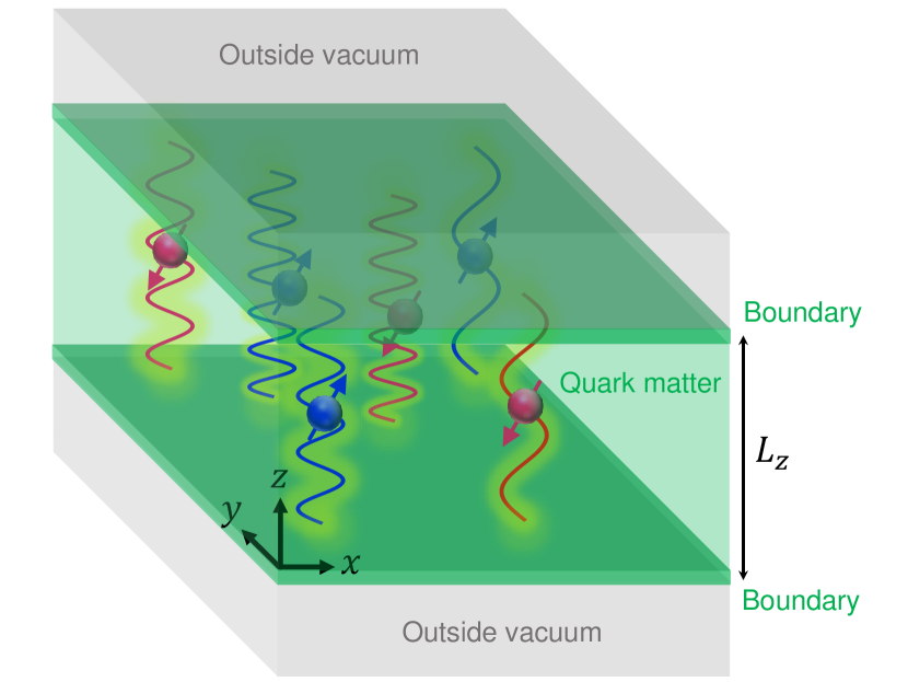
Figure 1: Schematics of the Casimir effect for quark fields inside thin quark matter, where the quark matter is confined between boundary conditions with a thickness $L_{z}$. The “outside vacuum” should be regarded as an arbitrary vacuum consistent with the boundary conditions.

Under these motivations, this paper focuses on what types of Casimir effects can occur in various phases of quark matter where the thickness of $z$ direction is extremely short (i.e., “thin” quark matter) as illustrated in Fig. 1. In particular, in this paper, we propose a QCD counterpart of the oscillating Casimir effect predicted in Weyl semimetals. This is realized for fermion fields in the dual chiral density wave (DCDW) phase [33] (also see Refs. [34, 35, 36, 37, 38, 39, 40, 41, 42, 43, 44, 45, 46, 47, 48, 49, 50, 51, 52, 53, 54, 55, 56, 57, 58, 59, 60, 61, 62, 63, 64, 65, 66, 67, 68, 69, 70, 71, 72, 73, 74, 75, 76, 77, 78, 79, 80] and Ref. [81] for a review). The DCDW phase is a candidate for the ground state of quark/nuclear matter in the density region of $\rho/\rho_{0}=3\sim 6$ with the normal nuclear density $\rho_{0}=0.16$ ${\rm fm}^{-3}$ [46, 47], and complex dispersion relations of fermions in this phase can be an origin of the oscillating Casimir effect.

In this paper, we aim to investigate types of Casimir effects induced from quark fields in dense quark matter. To accomplish this, this paper is organized as follows. In Sec. II, we formulate the zero-point energy and the Casimir energy within the Nambu–Jona-Lasinio (NJL) model [82, 83] as an effective model of QCD. In Sec. III, we show our numerical results and classify the types of Casimir effects in three density regions. Section IV is devoted to our conclusion and outlook.

II Formulation

II.1 Dual chiral density waves

A chiral density wave is a spatially inhomogeneous chiral condensate, which is represented as a position-dependent Lorentz-scalar condensate made of the Dirac fields, $\psi$ and $\bar{\psi}=\psi^{\dagger}\gamma_{0}$: $\langle\bar{\psi}\psi\rangle\propto\cos(\vec{q}\cdot\vec{r})$ with a wavenumber vector $\vec{q}$ and a position vector $\vec{r}$. Among various types of chiral density waves, in this study, we focus on the DCDW, where both the scalar and pseudoscalar condensates are position-dependent [33],

$$\langle\bar{\psi}\psi\rangle=\Delta\cos(\vec{q}\cdot\vec{r}),\ \ \ \langle\bar{\psi}i\gamma_{5}\psi\rangle=\Delta\sin(\vec{q}\cdot\vec{r}),$$ (1)

where $\Delta$ is the amplitude of the DCDW and is regarded as the radius of the chiral circle, $\langle\bar{\psi}\psi\rangle^{2}+\langle\bar{\psi}i\gamma_{5}\psi\rangle^{2}=\Delta^{2}$.

II.2 NJL model

To investigate the DCDW phase of quark matter, in this work, we use the NJL model [82, 83] (see Refs. [84, 85, 86, 87] for reviews), which was done in Refs. [41, 44, 46, 47] for early studies. The Lagrangian density of the two-flavor NJL model is written as

$$\mathcal{L}_{\rm NJL}=\bar{\psi}(i\partial\hbox to0.0pt{\hss/}+\mu\gamma_{0})\psi+G[(\bar{\psi}\psi)^{2}+(\bar{\psi}i\gamma_{5}\vec{\tau}\psi)^{2}],$$ (2)

where $\mu$ is the quark chemical potential, $G$ is the coupling constant of the four-point interactions, and $\vec{\tau}=(\tau_{1},\tau_{2},\tau_{3})$ is the Pauli matrix for the isospin. Here, we apply the mean-field ansatz for the DCDW,

$$\langle\bar{\psi}\psi\rangle=\Delta\cos(\vec{q}\cdot\vec{r}), \langle\bar{\psi}i\gamma_{5}\tau_{3}\psi\rangle=\Delta\sin(\vec{q}\cdot\vec{r}),$$ (3)

$$\langle\bar{\psi}i\gamma_{5}\tau_{1}\psi\rangle=0, \langle\bar{\psi}i\gamma_{5}\tau_{2}\psi\rangle=0,$$ (4)

where $\Delta$ is the amplitude of the DCDW, and $\vec{q}=(0,0,q)$ is the wavenumber of the DCDW propagating in the $z$ direction. Using this ansatz, the mean-field (MF) Lagrangian density is

$$\mathcal{L}_{\rm MF}= \bar{\psi}\big{[}i\partial\hbox to0.0pt{\hss/}+\mu\gamma_{0}-M\big{(}\cos(qz)+i\gamma_{5}\tau_{3}\sin(qz)\big{)}\big{]}\psi$$ (5)

$$-\frac{M^{2}}{4G},$$

where $M=-2G\Delta$.

Using a local chiral transformation (which may be called a Weinberg transformation), $\psi e^{i\gamma_{5}\tau_{3}qz/2}\to\psi_{\rm W}$, $\bar{\psi}e^{i\gamma_{5}\tau_{3}qz/2}\to\bar{\psi}_{\rm W}$, the original quark field $\psi$ is redefined as a new field $\psi_{\rm W}$, and the position dependence of the original Lagrangian (5) is removed in the redefined quark fields. Then, from the diagonalization of the inverse quark propagator in momentum space, we obtain the four eigenvalues of (quasi-)quarks, $\omega_{\pm}$ (the positive-energy modes if $\mu=0$) and $\tilde{\omega}_{\pm}$ (the negative-energy modes):

$$\omega_{\pm}=E_{s}-\mu,$$ (6)

$$\tilde{\omega}_{\pm}=-E_{s}-\mu,$$ (7)

where

$$E_{s}=\sqrt{k^{2}+M^{2}+q^{2}/4\pm\sqrt{(qk_{z})^{2}+M^{2}q^{2}}},$$ (8)

and $k^{2}=k_{x}^{2}+k_{y}^{2}+k_{z}^{2}$. When $q=0$, the dispersion relations return to those of usual massive quarks with a mass $M$, where the two modes with different spins are degenerate. When $q\neq 0$, the two modes are split, which is labeled by $s=\pm$. In this work, we focus on the case of $M<q/2$, which is a typical situation of the DCDW phase.

Using these eigenvalues, the thermodynamic potential (per a spatial volume $V=L_{x}L_{y}L_{z}$) at temperature $T=1/\beta$ is written as

$$\frac{\Omega(T)}{V}= -N_{f}N_{c}\int\frac{d^{3}k}{(2\pi)^{3}}\sum_{s=\pm}\left[E_{s}+\frac{1}{\beta}\ln\big{(}1+e^{-\beta(E_{s}-\mu)}\big{)}\right.$$

$$\left.+\frac{1}{\beta}\ln\big{(}1+e^{-\beta(E_{s}+\mu)}\big{)}\right]+\frac{M^{2}}{4G}.$$ (9)

In this work we fix the number of flavors as $N_{f}=2$ and the number of colors as $N_{c}=3$.

By taking the zero-temperature limit $T\rightarrow 0$ of the thermodynamic potential (9), we obtain

$$\frac{\Omega(T\to 0)}{V}\equiv\frac{E_{0}}{L_{z}}= -N_{f}N_{c}\int\frac{d^{3}k}{(2\pi)^{3}}\sum_{s=\pm}\left[E_{s}\right.$$

$$\left.+\left(\mu-E_{s}\right)\theta(\mu-E_{s})\right]+\frac{M^{2}}{4G}.$$ (10)

Here, the first term is regarded as the contribution from the Dirac sea, i.e., the negative zero-point energy from the fermion fields. The second term with the step function is the contribution from the Fermi sea of quarks. The third term is the positive energy from the order parameter $M$. To provide a Casimir-effect-like picture also for the Fermi sea contribution (as well as the Dirac sea), we have denoted Eq. (10) as $E_{0}/L_{z}$ where $E_{0}$ is the zero-point energy per unit area.

Note that in the traditional treatment of the NJL model, we determine the values of the order parameters $M$ and $q$ by minimizing Eq. (10) at a fixed $\mu$. In a finite volume, the thermodynamic potential in a fixed volume is minimized, and the values of $M$ and $q$ should be determined. This type of analysis is important for studying the phase diagram in finite volume, but it is not the purpose of this work. The purpose of this work is to investigate the feasibility of the oscillating Casimir effect in dense quark matter.

II.3 Casimir energy with Lifshitz formula

The Casimir energy is defined as a finite-volume effect for the zero-point energy (10). In a finite volume, the momentum integral with respect to the three-dimensional momentum of quarks in Eq. (10) is replaced by a discrete sum. In this paper, we impose the periodic boundary conditions (PBC) on quark fields at $z=0$ and $z=L_{z}$, where the $z$ component of quark momentum is discretized as $k_{z}\rightarrow 2n\pi/L_{z}$ where $n=0,1,\cdots,\infty$. Note that for the PBC, there is no outside vacuum as in Fig. 1, but the discretization of momentum (and corresponding eigenvalues) can induce a nonzero Casimir energy.

The zero-point energy (10) as the infinite integral and the corresponding infinite sum is divergent (unless an energy or a momentum cutoff is introduced), but the Casimir energy should be finite after using a mathematical technique. In this paper, we propose two approaches: (i) the Lifshitz formula and (ii) lattice regularizations.

Using the first approach, at zero temperature $T=0$ and zero chemical potential $\mu=0$, the analytical solution for the Casimir energy (per unit area) from quark fields in the DCDW phase can be written as

$$E_{\rm Cas} =-4N_{f}N_{c}\sum_{s=\pm}\int_{0}^{\infty}\frac{d\xi}{2\pi}\int\frac{dk_{x}dk_{y}}{(2\pi)^{2}}\ln\big{[}1-e^{-L_{z}k_{z}^{[s]}}\big{]},$$

$$k^{[\pm]}_{z} =\sqrt{k_{\perp}^{2}+M^{2}+\xi^{2}-\frac{q^{2}}{4}\mp iq\sqrt{k_{\perp}^{2}+\xi^{2}}},$$ (11)

where the first integral variable is the imaginary part $\xi$ of imaginary frequency $\omega\equiv i\xi$, and $k_{\perp}^{2}\equiv k_{x}^{2}+k_{y}^{2}$. The overall factor of $2N_{f}N_{c}$ means the degrees of freedom for particle-antiparticle, flavors, and colors, and the spin degrees of freedom are labeled as $s=\pm$. The overall factor of $-2$ and the factor of $-e^{-L_{z}k_{z}^{[s]}}$ are a property of the PBC on fermion fields. For the MIT bag boundary condition, see Appendix A.

Note that Eq. (11) is one of the main findings in this paper, which is an analog of the Lifshitz formula [88] to calculate the Casimir effect for photon fields. When we substitute $M=q=0$ and $q=0$, Eq. (11) returns to the formulas for the usual massless and massive quarks, respectively.

Furthermore, we define a dimensionless quantity, which we call the Casimir coefficient, by multiplying $L_{z}^{3}$,

$$C^{[3]}_{\rm Cas}\equiv L_{z}^{3}E_{\rm Cas}.$$ (12)

This is a convenient quantity for checking the $L_{z}$ dependence of the Casimir energy.

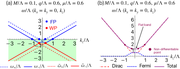
Figure 2: (a) Dispersion relations of the four eigenmodes, Eqs. (6) and (7), at $(M/\Lambda,q/\Lambda,\mu/\Lambda)=(0.1,0.6,0,6)$. (b) Each contribution from the Dirac sea (red line) or the Fermi sea (blue line) and their sum (purple line).

II.4 Casimir energy with a lattice regularization

As another approach to calculate the Casimir energy, we use lattice regularizations [89, 90, 28, 29, 91, 92, 30, 31, 93, 32, 94, 95, 96], which is regarded as a generalization of the original definition by Casimir [1]. Then, the Casimir energy (per unit area) on the three-dimensional lattice with a lattice spacing $a$ is defined as

$$E^{\rm Lat}_{\rm Cas}= E^{\rm sum}_{0}-E^{\rm int}_{0},$$ (13)

$$E^{\rm sum}_{0}= -\frac{N_{f}N_{c}}{a^{3}}\sum_{s=\pm}\int_{\rm BZ}\frac{d(ak_{x})d(ak_{y})}{(2\pi)^{2}}$$

$$\times\sum^{\rm BZ}_{n}\Big{[}\frac{1}{2}a|E^{\rm Lat}_{s,n}-\mu|+\frac{1}{2}a|E^{\rm Lat}_{s,n}+\mu|\Big{]},$$ (14)

$$E^{\rm int}_{0}= -\frac{N_{f}N_{c}}{a^{3}}\sum_{s=\pm}\int_{\rm BZ}\frac{d(ak_{x})d(ak_{y})d(ak_{z})}{(2\pi)^{3}}$$

$$\times N_{z}\Big{[}\frac{1}{2}a|E^{\rm Lat}_{s}-\mu|+\frac{1}{2}a|E^{\rm Lat}_{s}+\mu|\Big{]},$$ (15)

where the dispersion relations $E^{\rm Lat}_{\pm}$ on the lattice is obtained by replacing the original momenta $k^{2}_{i}$ ($i=x,y,z$) in Eqs. (6) and (7) as

$$k^{2}_{i}\rightarrow\frac{1}{a^{2}}(2-2\cos ak_{i}).$$ (16)

The first term $E^{\rm sum}_{0}$ in Eq. (13) is the zero-point energy in finite volume (and at finite chemical potential) with the momentum discretized by a finite thickness $L_{z}=aN_{z}$, where $N_{z}$ is the number of lattice cells. The second term $E^{\rm int}_{0}$ in Eq. (13) is the zero-point energy with the continuous momentum in infinite volume. The Casimir energy $E^{\rm Lat}_{\rm Cas}$ is defined as the difference between these two energies. Also, as a result of lattice regularization, the momentum integral and the momentum sum are taken within the first Brillouin zone (BZ). In the case of the PBC, the sum is over $n=0,1,...,N_{z}-1$ (or equivalently $n=0,1,...,N_{z}$).

Finally, we also define the dimensionless Casimir coefficient on the lattice,

$$C^{[3]{\rm Lat}}_{\rm Cas}\equiv L_{z}^{3}E^{\rm Lat}_{\rm Cas}=a^{3}N_{z}^{3}E^{\rm Lat}_{\rm Cas}.$$ (17)

The quantities on the lattice, $E^{\rm Lat}_{\rm Cas}$ and $C^{[3]{\rm Lat}}_{\rm Cas}$, depend on the lattice spacing $a$, but its continuum limit ($a\to 0$) should coincide with Eqs. (11) and (12) in the continuum theory (if the lattice regularization is appropriate):

$$C^{[3]}_{\rm Cas}=\lim_{a\to 0}C^{[3]{\rm Lat}}_{\rm Cas}.$$ (18)

II.5 Dispersion relations

We remark on the dispersion relations (6) and (7) for quark fields in the DCDW phase. In Fig. 2(a), we show the four eigenmodes in the DCDW phase. Here, the parameters are fixed as ($M/\Lambda,q/\Lambda,\mu/\Lambda,)=(0.1,0.6,0.6)$, where each quantity is dimensionless by dividing by a dimensional parameter $\Lambda$. In this figure, the two touching points of $\omega_{-}$ and $\tilde{\omega}_{-}$ are regarded as Weyl points, and in addition, $\omega_{-}$ intersects the Fermi level at the Fermi points (FPs). Furthermore, $\omega_{+}$ also intersects the Fermi level. Now, since we set $q=\mu$ for simplicity, the momenta of the Weyl points of $\omega_{-}$ and the intersection between the Fermi level and $\omega_{+}$ coincide.

Figure 2(b) shows each contribution from the Dirac or Fermi sea and their sum. The Dirac-sea and Fermi-sea contributions correspond to the absolute value of the first and second terms of the integrand in Eq. (10), respectively. These dispersion relations become flat bands at low momentum and bend twice in the middle of the dispersion relation. Such non-differentiable points in the dispersion relation generally lead to an oscillating Casimir effect.

In the next section, we will show plots as shown in Fig. 2(b) for intuitively understanding the mechanism of the Casimir effect.

III Results

In this section, we show the results for the Casimir coefficients in the low-, intermediate-, and high-density regions, with the PBC (see Appendix A for the discussion with the MIT bag boundary condition). In the following, with $\Lambda=860\ {\rm MeV}$, we fix the values of the order parameters, $M$ and $q$, at three $\mu$ (low-, intermediate, and high-density regions) as those obtained in Ref. [46], where the authors applied the mean-field approach in the NJL model with the proper-time regularization.

III.1 Oscillating Casimir effect (virtual parameters)

We will see in the following section that the oscillating Casimir effect is attributed to the flat band effect in the total dispersion relation caused by the presence of Weyl points. Therefore, in this subsection, we show how the flat band induces the oscillating Casimir effect by using a virtual parameter set that is not a solution to the gap equation of the NJL model but gives a typical flat band.

As typical parameters, we consider $(M/\Lambda,q/\Lambda)=(0.1,0.6)$, as shown in Fig. 2. Then, the Casimir coefficient defined as Eq. (12) is shown in Fig. 3. The obtained results show the oscillating Casimir effect. The Casimir energy is obtained from the difference between the momentum integral of the dispersion relation and the infinite sum of the momentum discretized by the boundary conditions. The oscillation of Casimir energy arises from the matching of the Weyl points and the discrete levels.

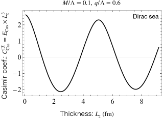
Figure 3: An example of the Casimir coefficient for the oscillating Casimir effect from the Dirac-sea contribution, where we fix $(M/\Lambda,q/\Lambda)=(0.1,0.6)$ as virtual parameters.

In order to intuitively understand the mechanism of oscillations, we provide a graphical explanation. In the following explanation, as shown in Fig. 4, we represent $E_{0}^{\rm sum}$ by the sum of the blue rectangular areas $S^{\rm sum}_{n}$, while the corresponding $E_{0}^{\rm int}$ is the sum of the red areas $S^{\rm int}_{n}$.

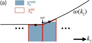
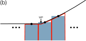
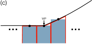
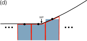
Figure 4: Graphical explanation for the oscillating Casimir effect. The sum of the blue rectangles $S^{\rm sum}_{n}$ and the integral over the red areas $S^{\rm int}_{n}$ correspond to the zero-point energies, $E_{0}^{\rm sum}$ and $E_{0}^{\rm int}$ in finite and infinite volumes, respectively. The Casimir energy is defined as $E_{0}^{\rm sum}-E_{0}^{\rm int}$, which corresponds to $\sum_{n}S^{\rm sum}_{n}-\sum_{n}S^{\rm int}_{n}$.

For example, in the low-momentum region of a massive particle, since the dispersion relation is a downward convex function, then $S^{\rm int}_{n}>S^{\rm sum}_{n}$ is satisfied, leading to a positive contribution to $N_{z}(S^{\rm sum}_{n}-S^{\rm int}_{n})\propto E^{\rm Lat}_{\rm Cas}$. On the other hand, in the high-momentum region, since the dispersion relation is an upward convex function due to the lattice regularization, $S^{\rm sum}_{n}>S^{\rm int}_{n}$, which leads to a negative contribution to $E^{\rm Lat}_{\rm Cas}$. In a region that can be regarded as a linear dispersion, we have $S^{\rm sum}_{n}=S^{\rm int}_{n}$.

As a crucial situation in this paper, in the flat-band region, it is also obvious that $S^{\rm sum}_{n}=S^{\rm int}_{n}$. The only exception is the case containing a Weyl point, where the corresponding areas are denoted as $S^{\rm sum}_{\rm W}$ and $S^{\rm int}_{\rm W}$. As the thickness $N_{z}$ increases, the position of the Weyl point relative to a rectangle changes. The case where the endpoint of a rectangle coincides with the Weyl point is shown in Fig. 4(a). In this case, if the dispersion relation around the Weyl point is assumed to be linear, then $S^{\rm sum}_{n}=S^{\rm int}_{n}$ is exactly held. Precisely speaking, it deviates somewhat from the linear dispersion and yields minor contributions as discussed in the last paragraph. As $N_{z}$ increases, the size and positions of rectangles change and reach the case shown in Fig. 4(b). In this case, we always have $S^{\rm int}_{n}>S^{\rm sum}_{n}$, and $E^{\rm Lat}_{\rm Cas}$ increases with $N_{z}$. As we continue to increase $N_{z}$, we eventually reach the case shown in Fig. 4(c), where the Weyl point coincides with the midpoint of the rectangle’s edge. In this case, $S^{\rm sum}_{\rm W}$ goes under the flat band, which maximizes $E^{\rm Lat}_{\rm Cas}$. Furthermore, as $N_{z}$ increases, the rectangle and the Weyl point reach the situation shown in Fig. 4(d). In this case, the excess of $S^{\rm int}_{\rm W}$ decreases and eventually reaches zero. Further increasing $N_{z}$, the position of the Weyl point for the rectangle returns to the case of Fig. 4(a).

Because the process from (a) to (d) occurs periodically, so that the value of $E^{\rm Lat}_{\rm Cas}$ oscillates with $L_{z}$. This is the origin of the $L_{z}$-dependent oscillation of Casimir energy. Then, the oscillation period (for the PBC) with respect to $L_{z}$ is written as [31]

$$L_{z}^{\rm osc}=\frac{2\pi}{k_{\rm WP}},$$ (19)

where $k_{\rm WP}$ is the momentum separation between the Weyl point and the origin. For the current parameters, the period is estimated to be $L_{z}^{\rm osc}\sim 5.1$ fm with $k_{\rm WP}/\Lambda\sim 0.283$, which is consistent with the plot in Fig. 3. In addition, in the $3+1$ dimensions, the minor deviation from this naive estimate is caused by the integral over the $k_{x}\neq 0$ and $k_{y}\neq 0$.

III.2 Low-density region

First, we consider the Casimir effect in the low-chemical potential region, where we fix $\mu/\Lambda=0.46$. In this region, we find a chiral condensed phase with $M/\Lambda=0.47$, but the DCDW phase has not yet developed $(q=0)$.

Figure 5 shows the dispersion relation of the quark field along the momentum $k_{z}$ on the lattice with $a\Lambda=1$, where the blue line represents the contribution from the Dirac sea, the red line from the Fermi sea, and the purple line their sum.

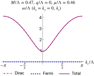
Figure 5: Dispersion relations on the lattice with $a\Lambda=1$ in the low-density region ($\mu/\Lambda=0.46$).

In this case, there is no mode crossing the Fermi level, which means that the total dispersion relation has no non-differentiable point. Therefore, the four dispersion relations are nothing but that of a massive Dirac fermion.

Figure 6 shows the results for the Casimir coefficient at $(M/\Lambda,q/\Lambda,\mu/\Lambda)=(0.47,0,0.46)$, obtained from the two approaches.

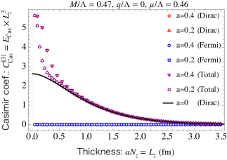
Figure 6: Casimir coefficients in the low-density region. We denote $a\Lambda$ as $a$ in the legends.

The resultant Casimir effect occurs only from the contribution of the Dirac sea. On the other hand, there is no contribution to the Casimir effect from the Fermi sea, as expected. In this figure, we find that $C^{[3]}_{\rm Cas}$ approaches zero in the long-thickness region. This behavior means that the damping of the Casimir energy $E_{\rm Cas}$ is faster than $1/L_{z}^{3}$ ($1/L_{z}^{3}$ is expected for the massless fields in the three-dimensional space). Such a faster damping is well known for free massive fields [97, 98, 99].

We present results for the two cases of lattice spacing $a\Lambda=0.2,0.4$ in Fig. 6. We show analytical solutions for only the Dirac-sea part of the Casimir coefficient, obtained from the Lifshitz formula. We observe that in the long-thickness region of about $aN_{z}=L_{z}>1.0\ {\rm fm}$, the lattice regularization works well even for $a\Lambda=0.4$. On the other hand, in the short-thickness region, the results for $a\Lambda=0.4$ deviate from the analytical solution due to the enhanced ultraviolet lattice cutoff effect. On the other hand, the results for $a\Lambda=0.2$ reproduce the analytical solution well up to about $aN_{z}=L_{z}=0.5\ {\rm fm}$. This result guarantees that the results from our lattice regularization are accurate up to a quite short-thickness region.

III.3 Intermediate-density region

As the chemical potential increases, the contribution from the quark Fermi sea causes a significant change in the behavior of the Casimir effect. Figure 7 shows the dispersion relation of the quark field along the momentum $k_{z}$ for fixed parameters $(M/\Lambda,q/\Lambda,\mu/\Lambda)=(0.46,0,0.485)$ and $a\Lambda=1$. In this parameter set, the DCDW phase has not yet occurred, but the $\omega_{\pm}$ with low momentum is below the Fermi sea. Then, there is an additional contribution to the Casimir effect from the Fermi sea as well as from the Dirac sea. Furthermore, the crossing points (Fermi points) of $\omega_{\pm}$ and the Fermi level lead to non-differentiable points in the total dispersion relation. Due to this, the oscillating Casimir effect occurs, by a mechanism similar to that discussed in the subsection II.5.

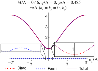
Figure 7: Dispersion relations on the lattice with $a\Lambda=1$ in the intermediate-density region ($\mu/\Lambda=0.485$).

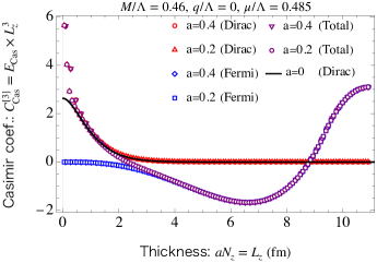
Figure 8: Casimir coefficients in the intermediate-density region. We denote $a\Lambda$ as $a$ in the legends.

Figure 8 shows the results for the Casimir coefficient. In the short thickness of Fig. 8, we find that the Casimir coefficient is dominated by the contribution from the Dirac sea, which is qualitatively the same as the result shown in the previous subsection III.2. On the other hand, in the long thickness of Fig. 8, the Casimir coefficient is dominated by the contribution from the Fermi sea. As a result, the sign of the total Casimir coefficient flips around $aN_{z}=L_{z}\sim 2.3\ {\rm fm}$ and $8.8\ {\rm fm}$. At further long-thickness, we expect an oscillation of the Casimir coefficient. However, now we do not show the numerical results due to the limitations of calculations with sufficient accuracy. By using Eq. (19), the period of oscillation is estimated to be $L_{z}^{\rm osc}=2\pi/k_{\rm FP}\sim 9.4\ {\rm fm}$, where $k_{\rm FP}/\Lambda\sim 0.154$ is the momentum of the Fermi point.

III.4 high-density region

When the chemical potential is large enough, the DCDW phase ($q\neq 0$) is realized. Figure 9 shows the dispersion relation of the quark fields along the momentum $k_{z}$ for fixed parameters $(M/\Lambda,q/\Lambda,\mu/\Lambda)=(0.09,0.62,0.72)$ with $a\Lambda=1$.

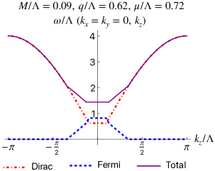
Figure 9: Dispersion relations on the lattice with $a\Lambda=1$ in the high-density region ($\mu/\Lambda=0.72$).

In this case, the two touching points of $\omega_{-}$ and $\tilde{\omega}_{-}$ are regarded as the Weyl points. Furthermore, the $\omega_{+}$ and $\omega_{-}$ cross the Fermi level. Thus, there are six non-differentiable points. In the low-momentum region, the total dispersion relation becomes a flat band due to the cancellations between $\omega_{-}$ and $\tilde{\omega}_{-}$ and between $\omega_{+}$ and $\tilde{\omega}_{+}$, and the edges of the flat band of the total dispersion relation are non-differentiable. Furthermore, due to the four Fermi points, the total dispersion relation is non-differentiable at the four momenta.

Figure 10 shows the results for the Casimir coefficient.

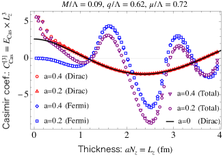
Figure 10: Casimir coefficients in the high-density region. We denote $a\Lambda$ as $a$ in the legends.

For the Dirac-sea effect, the Casimir effect shows oscillating behavior, as expected from the Weyl points. On the other hand, for the Fermi-sea effect as depicted by the red line, we see that the Fermi-sea part of Casimir coefficient oscillates with higher frequency than that from the Dirac sea. Its frequency is determined by the positions of the non-differentiable points on the dispersion relation. By using Eq. (19), the oscillation periods are estimated to be $L_{z}^{\rm osc}=2\pi/k_{\rm WP}\sim 4.9$ fm with $k_{\rm WP}/\Lambda\sim 0.297$ (for the Dirac sea part) and $L_{z}^{\rm osc}=2\pi/k_{\rm FP}\sim 1.4$ fm with $k_{\rm FP}/\Lambda\sim 1.03$ (for the Fermi sea part of $\omega_{-}$), and $L_{z}^{\rm osc}=2\pi/k_{\rm FP}\sim 3.6$ fm with $k_{\rm FP}/\Lambda\sim 0.40$ (for the Fermi sea part of $\omega_{+}$). The Dirac-sea and Fermi-sea contributions shown in Fig. 10 are dominated by the periods of $L_{z}^{\rm osc}\sim 4.9$ fm and $L_{z}^{\rm osc}\sim 1.4$ fm, respectively, and the total result is their superposition.

IV Conclusion and outlook

In this paper, we have discussed the Casimir effect from quark fields in some phases of quark matter. In particular, we consider the QCD counterpart of a new type of Casimir effect i.e., the oscillating Casimir effect. We have classified the typical behaviors of the Casimir effect by focusing on the three types of density regions:

1. When the quark chemical potential is small enough, the quark-number density is zero. Then, the Casimir effect for massive quark fields occurs, where the damping of the Casimir energy with increasing thickness is characterized by the dynamical masses of quarks.

2. As the quark chemical potential increases, the quark number density becomes nonzero. In this region, the contribution from the quark Fermi sea effect leads to the oscillating Casimir effect.

3. Further increasing the chemical potential eventually leads to a phase transition into the DCDW phase. In this region, in addition to the Fermi sea effect, the Weyl-point structure of quark fields in the DCDW phase results in the oscillating Casimir effect. The total Casimir energy behaves as the superposition of two types of oscillations.

To clarify terminology, one of our main findings may be called the DCDW-induced oscillating Casimir effect, which is a kind of the WP-induced oscillating Casimir effect predicted in Ref. [31]. On the other hand, the FP-induced oscillating Casimir effect would be a common term for general fermionic systems at finite density in finite volume.

In the following, we list some potential future studies.

• Solving gap equation in finite volume—In this work, we input the values of order parameters obtained from the gap equation in infinite volume, in order to understand the typical behavior of the Casimir effect for typical dispersion relations. As a more precise analysis, one can calculate the order parameters by minimizing the thermodynamic or effective potential in finite volume, and then one can understand the self-consistent relationship between the volume-dependent order parameters and the Casimir effect. This type of study would help elucidate the phase diagram of interacting fermions in finite volume (e.g., see Refs. [100, 101, 102, 103, 104, 105, 106, 107]) from the viewpoint of the Casimir effect.

• Lattice simulations—Our predictions will be examined by future lattice NJL (and also QCD) simulations. Since Monte Carlo simulations at large quark chemical potential suffer from the sign-problem, sign-problem-free techniques should be applied. In particular, numerical simulations of Casimir effects for lattice gauge fields have been vigorously studied, such as the U(1) gauge [108, 109, 110], the compact U(1) gauge [111, 112, 113, 114, 115], the SU(2) gauge [116, 117], and the SU(3) gauge fields [118, 119], so that the interplay between quark and gluon dynamics would be interesting.

• Finite temperature—At finite temperature, thermal fluctuations (as well as quantum fluctuations) also induce the Casimir effect, which is the so-called thermal Casimir effect well established theoretically [88] and experimentally [120]. The Casimir energy at finite temperature can be calculated by using a straightforward modification of Eq. (11) or Eq. (13). Although the DCDW phase disappears at sufficiently high temperature, in the low-temperature region the oscillating Casimir effect can be realized.

• Axion electrodynamics—In this work, we consider only the Casimir effect for quark fields, which is induced by boundary conditions on quark fields. The dynamics of photons in the DCDW phase may be described by modified Maxell equations [63, 121, 76] which is the so-called axion electrodynamics [122, 123]. The Casimir energy for such modified photon fields can exhibit a sign-flipping behavior [19, 124, 125, 126, 127, 95] when boundary conditions on photon fields are imposed. It will be interesting whether or not such a photonic Casimir effect occurs also in the DCDW phase.

• Models with nucleons—In this work, we consider the Casimir effect for quark degrees of freedom based on the NJL model. Apart from the NJL model, in the low-density phase of QCD, relevant degrees of freedom are hadrons, specifically nucleons. Therefore, it will be important to examine the consistency between the quark Casimir effect in the NJL model and the nucleon Casimir effect in an effective model such as the nucleon linear sigma model which can also investigate the DCDW phase.

• Other inhomogeneous chiral phases—We have shown the WP-induced oscillating Casimir effect in the DCDW phase, which is particular to systems with momentum-dependent Weyl points. It would be interesting what types of Casimir effects can occur in other inhomogeneous chiral phases. For example, the real-kink crystal phase is known as a possible ground state in the 3+1 dimension NJL model [50]. In this phase, because $k_{z}$ is not a conserved quantity, our approach formulated in spatial-momentum space cannot be applied, but the Casimir energy should be calculated by approaches formulated with discrete eigenenergies. Furthermore, apart from the dense quark matter, a magnetic field can also induce the DCDW phase [53], which is the so-called magnetic dual chiral density wave (MDCDW) (see Ref. [128] for a review). The Casimir effect in such a phase is also interesting.

• Lower-dimensional models of QCD—The WP-induced oscillating Casimir effect can occur also in lower spatial dimensions (i.e., $1+1$ or $2+1$ dimensions) [31]. Therefore, investigation of the Casimir effect in possible inhomogeneous phases of low-dimensional QCD-like models, such as the Gross-Neveu model [129, 130, 131], the chiral Gross-Neveu (NJL₂) model [132], and the ’t Hooft model (QCD₂) [132, 133, 134], will be also important.

Appendix A Results with MIT bag boundary

In the main text, we applied the PBC to consider the Casimir effect. In this Appendix, we consider the case with the MIT bag boundary condition, which is more realistic when we consider quark matter in nature or experiments.

The MIT bag boundary condition [135] requires that the quark-current flux toward normal to the boundary is zero. For the massless Dirac field on the MIT bag boundaries, one can obtain the discretized momentum $k_{z}\to(n+1/2)\pi/L_{z}$ as an analytic solution satisfying the Dirac equation. On the other hand, for the massive case, one cannot obtain an analytic form of momentum, so that one should apply an alternative approach with no analytic form of $k_{z}$ (e.g., Refs. [136, 137, 138]). In this Appendix, as an approximate estimate, we show the results using the massless solution $k_{z}\to(n+1/2)\pi/L_{z}$, which may be called “MIT bag” boundary conditions.

The Lifshitz formula for the Casimir energy from the Dirac sea with the “MIT bag” boundaries is given by

$$E_{\rm Cas}^{\rm``MIT"} =-2N_{f}N_{c}\sum_{s=\pm}\int_{0}^{\infty}\frac{d\xi}{2\pi}\int\frac{d^{2}k_{\perp}}{(2\pi)^{2}}\ln\big{[}1+e^{-2L_{z}k_{z}^{[s]}}\big{]},$$

$$k^{[\pm]}_{z} =\sqrt{k_{\perp}^{2}+M^{2}+\xi^{2}-\frac{q^{2}}{4}\mp iq\sqrt{k_{\perp}^{2}+\xi^{2}}},$$ (20)

where the first integral variable is the imaginary part $\xi$ of imaginary frequency $\omega\equiv i\xi$, $k_{\perp}^{2}\equiv k_{x}^{2}+k_{y}^{2}$, and $d^{2}k_{\perp}\equiv dk_{x}dk_{y}$. The overall factor of $2N_{f}N_{c}$ means the degrees of freedom for particle-antiparticle, flavors, and colors, and the spin degrees of freedom are labeled as $s=\pm$. The overall minus sign and the factor of $+e^{-2L_{z}k_{z}^{[s]}}$ is a property of the “MIT bag” boundary on fermion fields. In the lattice rugularization, we have to replace as $\sum^{\rm BZ}_{n}\to\frac{1}{2}\sum^{\rm BZ}_{n}$ in Eq. (14), and the sum is over $n=0,1,...,2N_{z}-1$.

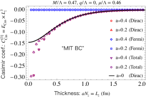
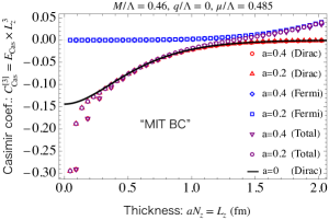
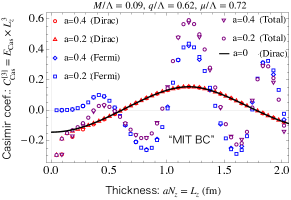
Figure 11: Casimir coefficients in the low-density region with the “MIT bag” boundary conditions. We denote $a\Lambda$ as $a$ in the legends.

Figure 11 shows the results of the Casimir coefficients at low-, intermediate-, and high-density regions. In the case of the “MIT bag” boundary, the number of discretized levels is twice larger than that with the PBC. As a result, the period of oscillation is half of that with the PBC: analogous to Eq. (19),

$$L_{z}^{\rm osc``MIT"}=\frac{\pi}{k_{\rm WP}}.$$ (21)

Furthermore, from these results, we can also discuss the case with the antiperiodic boundary conditions (APBCs). The discrete momentum, $k_{z}\to(2n+1)\pi/L_{z}$, for the APBCs is shifted by a half period from $k_{z}\to 2n\pi/L_{z}$ for the PBCs, and hence the sign of the Casimir energy is flipped and also its absolute value changes slightly. The corresponding Lifshitz formula is written as

$$E_{\rm Cas}^{\rm APBC} =-4N_{f}N_{c}\sum_{s=\pm}\int_{0}^{\infty}\frac{d\xi}{2\pi}\int\frac{d^{2}k_{\perp}}{(2\pi)^{2}}\ln\big{[}1+e^{-L_{z}k_{z}^{[s]}}\big{]}.$$ (22)

In the $3+1$ dimensions, the Casimir energy with $k_{z}\to(2n+1)\pi/L_{z}$ is $16$ times larger than that with $k_{z}\to(n+1/2)\pi/L_{z}$. As a result, by multiplying the vertical axis obtained in Fig. 11 by $16$ and the horizontal axis by $2$, we can obtain the exact results for the APBCs.

References

- Casimir [1948] H. B. G. Casimir, On the Attraction Between Two Perfectly Conducting Plates, Proc. Kon. Ned. Akad. Wetensch. 51, 793 (1948).
- Plunien et al. [1986] G. Plunien, B. Müller, and W. Greiner, The Casimir Effect, Phys. Rep. 134, 87 (1986).
- Mostepanenko and Trunov [1988] V. M. Mostepanenko and N. N. Trunov, The Casimir Effect and Its Applications, Sov. Phys. Usp. 31, 965 (1988).
- Bordag et al. [2001] M. Bordag, U. Mohideen, and V. M. Mostepanenko, New developments in the Casimir effect, Phys. Rep. 353, 1 (2001), arXiv:quant-ph/0106045 [quant-ph] .
- Milton [2001] K. A. Milton, The Casimir Effect: Physical Manifestations of Zero-Point Energy (World Scientific, Singapore, 2001).
- Klimchitskaya et al. [2009] G. L. Klimchitskaya, U. Mohideen, and V. M. Mostepanenko, The Casimir force between real materials: Experiment and theory, Rev. Mod. Phys. 81, 1827 (2009), arXiv:0902.4022 [cond-mat.other] .
- Lamoreaux [1997] S. K. Lamoreaux, Demonstration of the Casimir Force in the 0.6 to Range, Phys. Rev. Lett. 78, 5 (1997), [Erratum: Phys. Rev. Lett. 81, 5475 (1998)].
- Bressi et al. [2002] G. Bressi, G. Carugno, R. Onofrio, and G. Ruoso, Measurement of the Casimir force between parallel metallic surfaces, Phys. Rev. Lett. 88, 041804 (2002), arXiv:quant-ph/0203002 .
- Gong et al. [2021] T. Gong, M. R. Corrado, A. R. Mahbub, C. Shelden, and J. N. Munday, Recent progress in engineering the Casimir effect – applications to nanophotonics, nanomechanics, and chemistry, Nanophotonics 10, 523 (2021).
- Dzyaloshinskii et al. [1961] I. E. Dzyaloshinskii, E. M. Lifshitz, and L. P. Pitaevskii, The general theory of van der Waals forces, Adv. Phys. 10, 165 (1961).
- Boyer [1974] T. H. Boyer, Van der Waals forces and zero-point energy for dielectric and permeable materials, Phys. Rev. A 9, 2078 (1974).
- Kenneth et al. [2002] O. Kenneth, I. Klich, A. Mann, and M. Revzen, Repulsive Casimir forces, Phys. Rev. Lett. 89, 033001 (2002), arXiv:quant-ph/0202114 .
- Munday et al. [2009] J. N. Munday, F. Capasso, and V. A. Parsegian, Measured long-range repulsive Casimir–Lifshitz forces, Nature 457, 170 (2009).
- Henkel and Joulain [2005] C. Henkel and K. Joulain, Casimir force between designed materials: what is possible and what not, EPL 72, 929 (2005), arXiv:quant-ph/0407153 .
- Rosa et al. [2008] F. S. S. Rosa, D. A. R. Dalvit, and P. W. Milonni, Casimir-Lifshitz Theory and Metamaterials, Phys. Rev. Lett. 100, 183602 (2008), arXiv:0803.2908 [quant-ph] .
- Grushin and Cortijo [2011] A. G. Grushin and A. Cortijo, Tunable Casimir Repulsion with Three Dimensional Topological Insulators, Phys. Rev. Lett. 106, 020403 (2011), arXiv:1002.3481 [cond-mat.mtrl-sci] .
- Tse and MacDonald [2012] W.-K. Tse and A. H. MacDonald, Quantized Casimir Force, Phys. Rev. Lett. 109, 236806 (2012), arXiv:1208.3786 [cond-mat.mes-hall] .
- Wilson et al. [2015] J. H. Wilson, A. A. Allocca, and V. Galitski, Repulsive casimir force between weyl semimetals, Phys. Rev. B 91, 235115 (2015), arXiv:1501.07659 [cond-mat.mes-hall] .
- Fukushima et al. [2019] K. Fukushima, S. Imaki, and Z. Qiu, Anomalous Casimir effect in axion electrodynamics, Phys. Rev. D 100, 045013 (2019), arXiv:1906.08975 [hep-th] .
- Fuchs et al. [2007] J. N. Fuchs, A. Recati, and W. Zwerger, Oscillating Casimir force between impurities in one-dimensional Fermi liquids, Phys. Rev. A 75, 043615 (2007), arXiv:cond-mat/0610659 [cond-mat.mes-hall] .
- Wächter et al. [2007] P. Wächter, V. Meden, and K. Schönhammer, Indirect forces between impurities in one-dimensional quantum liquids, Phys. Rev. B 76, 045123 (2007), arXiv:cond-mat/0703128 [cond-mat.str-el] .
- Kolomeisky et al. [2008] E. B. Kolomeisky, J. P. Straley, and M. Timmins, Casimir effect in a one-dimensional gas of free fermions, Phys. Rev. A 78, 022104 (2008), arXiv:0706.2887 [cond-mat.mes-hall] .
- Zhabinskaya and Mele [2009] D. Zhabinskaya and E. J. Mele, Casimir interactions between scatterers in metallic carbon nanotubes, Phys. Rev. B 80, 155405 (2009), arXiv:0909.1731 [cond-mat.mes-hall] .
- Chen et al. [2012] L.-W. Chen, G.-Z. Su, J.-C. Chen, and A. Bjarne, Oscillating Casimir force between two slabs in a Fermi sea, Chin. Phys. B 21, 010501 (2012).
- Chen [2011] S. G. C. J. Chen, L., Oscillating Casimir effect of a trapped Fermi gas, J. Stat. Phys. 143, 523 (2011).
- [26] A. Han, Seyit Deniz and E. Aydiner, Oscillating Casimir force of trapped Bose gas in electromagnetic field, arXiv:1508.01040 [quant-ph] .
- Jiang and Wilczek [2019] Q.-D. Jiang and F. Wilczek, Chiral Casimir forces: Repulsive, enhanced, tunable, Phys. Rev. B 99, 125403 (2019), arXiv:1805.07994 [cond-mat.mes-hall] .
- Ishikawa et al. [2020] T. Ishikawa, K. Nakayama, and K. Suzuki, Casimir effect for lattice fermions, Phys. Lett. B 809, 135713 (2020), arXiv:2005.10758 [hep-lat] .
- Ishikawa et al. [2021] T. Ishikawa, K. Nakayama, and K. Suzuki, Lattice-fermionic Casimir effect and topological insulators, Phys. Rev. Res. 3, 023201 (2021), arXiv:2012.11398 [hep-lat] .
- Mandlecha and Gavai [2022] Y. V. Mandlecha and R. V. Gavai, Lattice fermionic Casimir effect in a slab bag and universality, Phys. Lett. B 835, 137558 (2022), arXiv:2207.00889 [hep-lat] .
- Nakayama and Suzuki [2023a] K. Nakayama and K. Suzuki, Dirac/Weyl-node-induced oscillating Casimir effect, Phys. Lett. B 843, 138017 (2023a), arXiv:2207.14078 [cond-mat.mes-hall] .
- [32] K. Nakata and K. Suzuki, Non-Hermitian Casimir Effect of Magnons, arXiv:2305.09231 [quant-ph] .
- Dautry and Nyman [1979] F. Dautry and E. M. Nyman, Pion condensation and the -model in liquid neutron matter, Nucl. Phys. A 319, 323 (1979).
- Broniowski and Kutschera [1990a] W. Broniowski and M. Kutschera, One fermion loop contribution to the energy of the neutral pion condensate in the Model, Phys. Lett. B 234, 449 (1990a).
- Kutschera et al. [1990a] M. Kutschera, W. Broniowski, and A. Kotlorz, Quark matter with neutral pion condensate, Phys. Lett. B 237, 159 (1990a).
- Broniowski and Kutschera [1990b] W. Broniowski and M. Kutschera, One-loop effective action in the model for a periodic-chiral-field ansatz, Phys. Rev. D 41, 3800 (1990b).
- Broniowski and Kutschera [1990c] W. Broniowski and M. Kutschera, Ambiguities in effective chiral models with cutoff, Phys. Lett. B 242, 133 (1990c).
- Kutschera et al. [1990b] M. Kutschera, W. Broniowski, and A. Kotlorz, Quark matter with pion condensate in an effective chiral model, Nucl. Phys. A 516, 566 (1990b).
- Kato et al. [1992] M. Kato, W. Bentz, and K. Tanaka, Neutral pion condensation in quark matter including vacuum fluctuation effects, Phys. Rev. C 45, 2445 (1992).
- Kotlorz and Kutschera [1994] A. Kotlorz and M. Kutschera, Quark matter inside neutron stars in an effective chiral model, Acta Phys. Polon. B 25, 859 (1994).
- Sadzikowski and Broniowski [2000] M. Sadzikowski and W. Broniowski, Nonuniform chiral phase in effective chiral quark models, Phys. Lett. B 488, 63 (2000), arXiv:hep-ph/0003282 .
- Takahashi and Tatsumi [2001a] K. Takahashi and T. Tatsumi, Solution of the Dirac equation with an axial vector current in the chiral model, Prog. Theor. Phys. 105, 437 (2001a).
- Takahashi and Tatsumi [2001b] K. Takahashi and T. Tatsumi, condensation at finite density in the linear model, Phys. Rev. C 63, 015205 (2001b).
- Sadzikowski [2003] M. Sadzikowski, Coexistence of pion condensation and color superconductivity in two flavor quark matter, Phys. Lett. B 553, 45 (2003), arXiv:hep-ph/0210065 .
- Takahashi [2002] K. Takahashi, Neutral pion condensation in the chiral model, Phys. Rev. C 66, 025202 (2002).
- [46] T. Tatsumi and E. Nakano, Dual chiral density wave in quark matter, arXiv:hep-ph/0408294 .
- Nakano and Tatsumi [2005] E. Nakano and T. Tatsumi, Chiral symmetry and density wave in quark matter, Phys. Rev. D 71, 114006 (2005), arXiv:hep-ph/0411350 .
- Sadzikowski [2006] M. Sadzikowski, Comparison of the non-uniform chiral and 2SC phases at finite temperatures and densities, Phys. Lett. B 642, 238 (2006), arXiv:hep-ph/0609186 .
- Bringoltz [2007] B. Bringoltz, Chiral crystals in strong-coupling lattice QCD at nonzero chemical potential, JHEP 03, 016, arXiv:hep-lat/0612010 .
- Nickel [2009] D. Nickel, Inhomogeneous phases in the Nambu–Jona-Lasino and quark-meson model, Phys. Rev. D 80, 074025 (2009), arXiv:0906.5295 [hep-ph] .
- Maedan [2010] S. Maedan, Influence of current mass on the spatially inhomogeneous chiral condensate, Prog. Theor. Phys. 123, 285 (2010), arXiv:0908.0594 [hep-ph] .
- Carignano et al. [2010] S. Carignano, D. Nickel, and M. Buballa, Influence of vector interaction and Polyakov loop dynamics on inhomogeneous chiral symmetry breaking phases, Phys. Rev. D 82, 054009 (2010), arXiv:1007.1397 [hep-ph] .
- Frolov et al. [2010] I. E. Frolov, V. C. Zhukovsky, and K. G. Klimenko, Chiral density waves in quark matter within the Nambu–Jona-Lasinio model in an external magnetic field, Phys. Rev. D 82, 076002 (2010), arXiv:1007.2984 [hep-ph] .
- Partyka and Sadzikowski [2011] T. L. Partyka and M. Sadzikowski, Chiral density waves in quarkyonic matter, Acta Phys. Polon. B 42, 1305 (2011), arXiv:1011.0921 [hep-ph] .
- Abuki et al. [2012] H. Abuki, D. Ishibashi, and K. Suzuki, Crystalline chiral condensates off the tricritical point in a generalized Ginzburg-Landau approach, Phys. Rev. D 85, 074002 (2012), arXiv:1109.1615 [hep-ph] .
- Carignano and Buballa [2012] S. Carignano and M. Buballa, Two-dimensional chiral crystals in the Nambu-Jona-Lasinio model, Phys. Rev. D 86, 074018 (2012), arXiv:1203.5343 [hep-ph] .
- Karasawa and Tatsumi [2015] S. Karasawa and T. Tatsumi, Variational approach to the inhomogeneous chiral phase in quark matter, Phys. Rev. D 92, 116004 (2015), arXiv:1307.6448 [hep-ph] .
- Müller et al. [2013] D. Müller, M. Buballa, and J. Wambach, Dyson-Schwinger study of chiral density waves in QCD, Phys. Lett. B 727, 240 (2013), arXiv:1308.4303 [hep-ph] .
- Heinz et al. [2015] A. Heinz, F. Giacosa, and D. H. Rischke, Chiral density wave in nuclear matter, Nucl. Phys. A 933, 34 (2015), arXiv:1312.3244 [nucl-th] .
- Moreira et al. [2014] J. Moreira, B. Hiller, W. Broniowski, A. A. Osipov, and A. H. Blin, Nonuniform phases in a three-flavor Nambu-Jona-Lasinio model, Phys. Rev. D 89, 036009 (2014), arXiv:1312.4942 [hep-ph] .
- Tatsumi and Muto [2014] T. Tatsumi and T. Muto, Quark beta decay in the inhomogeneous chiral phase and cooling of compact stars, Phys. Rev. D 89, 103005 (2014), arXiv:1403.1927 [nucl-th] .
- Carignano et al. [2014] S. Carignano, M. Buballa, and B.-J. Schaefer, Inhomogeneous phases in the quark-meson model with vacuum fluctuations, Phys. Rev. D 90, 014033 (2014), arXiv:1404.0057 [hep-ph] .
- Tatsumi et al. [2015] T. Tatsumi, K. Nishiyama, and S. Karasawa, Novel Lifshitz point for chiral transition in the magnetic field, Phys. Lett. B 743, 66 (2015), arXiv:1405.2155 [hep-ph] .
- Hayata and Yamamoto [2015] T. Hayata and A. Yamamoto, Inhomogeneous Polyakov loop induced by inhomogeneous chiral condensates, Phys. Lett. B 744, 401 (2015), arXiv:1408.1905 [hep-ph] .
- Harada et al. [2015] M. Harada, H. K. Lee, Y.-L. Ma, and M. Rho, Inhomogeneous quark condensate in compressed Skyrmion matter, Phys. Rev. D 91, 096011 (2015), arXiv:1502.02508 [hep-ph] .
- Lee et al. [2015] T.-G. Lee, E. Nakano, Y. Tsue, T. Tatsumi, and B. Friman, Landau-Peierls instability in a Fulde-Ferrell type inhomogeneous chiral condensed phase, Phys. Rev. D 92, 034024 (2015), arXiv:1504.03185 [hep-ph] .
- Nishiyama et al. [2015] K. Nishiyama, S. Karasawa, and T. Tatsumi, Hybrid chiral condensate in the external magnetic field, Phys. Rev. D 92, 036008 (2015), arXiv:1505.01928 [nucl-th] .
- Carignano et al. [2015] S. Carignano, E. J. Ferrer, V. de la Incera, and L. Paulucci, Crystalline chiral condensates as a component of compact stars, Phys. Rev. D 92, 105018 (2015), arXiv:1505.05094 [nucl-th] .
- Carlomagno et al. [2015] J. P. Carlomagno, D. Gómez Dumm, and N. N. Scoccola, Inhomogeneous phases in nonlocal chiral quark models, Phys. Rev. D 92, 056007 (2015), arXiv:1507.01560 [hep-ph] .
- Yoshiike et al. [2015] R. Yoshiike, K. Nishiyama, and T. Tatsumi, Spontaneous magnetization of quark matter in the inhomogeneous chiral phase, Phys. Lett. B 751, 123 (2015), arXiv:1507.02110 [hep-ph] .
- Heinz et al. [2016] A. Heinz, F. Giacosa, M. Wagner, and D. H. Rischke, Inhomogeneous condensation in effective models for QCD using the finite-mode approach, Phys. Rev. D 93, 014007 (2016), arXiv:1508.06057 [hep-ph] .
- Suenaga and Harada [2016] D. Suenaga and M. Harada, Appearance of novel modes of mesons with negative velocity in the dual chiral density wave, Phys. Rev. D 93, 076005 (2016), arXiv:1509.08578 [hep-ph] .
- Karasawa et al. [2016] S. Karasawa, T.-G. Lee, and T. Tatsumi, Brazovskii–Dyugaev effect on the inhomogeneous chiral transition in quark matter, PTEP 2016, 043D02 (2016).
- Adhikari et al. [2017] P. Adhikari, J. O. Andersen, and P. Kneschke, Inhomogeneous chiral condensate in the quark-meson model, Phys. Rev. D 96, 016013 (2017), [Erratum: Phys. Rev. D 98, 099902 (2018)], arXiv:1702.01324 [hep-ph] .
- Yoshiike et al. [2017] R. Yoshiike, T.-G. Lee, and T. Tatsumi, Chiral pair fluctuations for the inhomogeneous chiral transition, Phys. Rev. D 95, 074010 (2017), arXiv:1702.01511 [hep-ph] .
- Tatsumi et al. [2018] T. Tatsumi, R. Yoshiike, and K. Kashiwa, Anomalous Hall effect in dense QCD matter, Phys. Lett. B 785, 46 (2018), arXiv:1803.10514 [hep-ph] .
- Carignano and Buballa [2020] S. Carignano and M. Buballa, Inhomogeneous chiral condensates in three-flavor quark matter, Phys. Rev. D 101, 014026 (2020), arXiv:1910.03604 [hep-ph] .
- Lakaschus et al. [2021] P. Lakaschus, M. Buballa, and D. H. Rischke, Competition of inhomogeneous chiral phases and two-flavor color superconductivity in the NJL model, Phys. Rev. D 103, 034030 (2021), arXiv:2012.07520 [hep-ph] .
- Tabatabaee Mehr [2023] S. M. A. Tabatabaee Mehr, Chiral symmetry breaking and phase diagram of dual chiral density wave in a rotating quark matter, Phys. Rev. D 108, 094042 (2023), arXiv:2306.11753 [nucl-th] .
- Pitsinigkos and Schmitt [2024] S. Pitsinigkos and A. Schmitt, Chiral crossover versus chiral density wave in dense nuclear matter, Phys. Rev. D 109, 014024 (2024), arXiv:2309.01603 [nucl-th] .
- Buballa and Carignano [2015] M. Buballa and S. Carignano, Inhomogeneous chiral condensates, Prog. Part. Nucl. Phys. 81, 39 (2015), arXiv:1406.1367 [hep-ph] .
- Nambu and Jona-Lasinio [1961a] Y. Nambu and G. Jona-Lasinio, Dynamical Model of Elementary Particles Based on an Analogy with Superconductivity. I, Phys. Rev. 122, 345 (1961a).
- Nambu and Jona-Lasinio [1961b] Y. Nambu and G. Jona-Lasinio, Dynamical Model of Elementary Particles Based on an Analogy with Superconductivity. II, Phys. Rev. 124, 246 (1961b).
- Vogl and Weise [1991] U. Vogl and W. Weise, The Nambu and Jona Lasinio model: Its implications for hadrons and nuclei, Prog. Part. Nucl. Phys. 27, 195 (1991).
- Klevansky [1992] S. P. Klevansky, The Nambu–Jona-Lasinio model of quantum chromodynamics, Rev. Mod. Phys. 64, 649 (1992).
- Hatsuda and Kunihiro [1994] T. Hatsuda and T. Kunihiro, QCD phenomenology based on a chiral effective Lagrangian, Phys. Rept. 247, 221 (1994), arXiv:hep-ph/9401310 .
- Buballa [2005] M. Buballa, NJL model analysis of dense quark matter, Phys. Rept. 407, 205 (2005), arXiv:hep-ph/0402234 .
- Lifshitz [1956] E. M. Lifshitz, The theory of molecular attractive forces between solids, Sov. Phys. JETP 2, 73 (1956).
- Actor et al. [2000] A. Actor, I. Bender, and J. Reingruber, Casimir effect on a finite lattice, Fortsch. Phys. 48, 303 (2000), arXiv:quant-ph/9908058 [quant-ph] .
- [90] M. Pawellek, Finite-sites corrections to the Casimir energy on a periodic lattice, arXiv:1303.4708 [hep-th] .
- Nakayama and Suzuki [2023b] K. Nakayama and K. Suzuki, Remnants of the nonrelativistic Casimir effect on the lattice, Phys. Rev. Res. 5, L022054 (2023b), arXiv:2204.12032 [quant-ph] .
- Nakata and Suzuki [2023] K. Nakata and K. Suzuki, Magnonic Casimir Effect in Ferrimagnets, Phys. Rev. Lett. 130, 096702 (2023), arXiv:2205.13802 [quant-ph] .
- Swingle and Van Raamsdonk [2023] B. Swingle and M. Van Raamsdonk, Enhanced negative energy with a massless Dirac field, JHEP 08, 183, arXiv:2212.02609 [hep-th] .
- [94] E. Flores, C. Ireland, N. Jamhour, V. Lasasso, N. Kurth, and M. Leinbach, Casimir force in discrete scalar fields I: 1D and 2D cases, arXiv:2309.00624 [quant-ph] .
- [95] K. Nakayama and K. Suzuki, Casimir effect in axion electrodynamics with lattice regularizations, arXiv:2310.18092 [hep-th] .
- [96] C. W. J. Beenakker, Topologically protected Casimir effect for lattice fermions, arXiv:2402.02477 [quant-ph] .
- Bender and Hays [1976] C. M. Bender and P. Hays, Zero Point Energy of Fields in a Finite Volume, Phys. Rev. D 14, 2622 (1976).
- Hays [1979] P. Hays, Vacuum fluctuations of a confined massive field in two dimensions, Annals Phys. 121, 32 (1979).
- Ambjørn and Wolfram [1983] J. Ambjørn and S. Wolfram, Properties of the vacuum. I. Mechanical and thermodynamic, Annals Phys. 147, 1 (1983).
- Kim et al. [1987] S. K. Kim, W. Namgung, K. S. Soh, and J. H. Yee, Dynamical symmetry breaking and space-time topology, Phys. Rev. D 36, 3172 (1987).
- Braun et al. [2005] J. Braun, B. Klein, and H. J. Pirner, Volume dependence of the pion mass in the quark-meson-model, Phys. Rev. D 71, 014032 (2005), arXiv:hep-ph/0408116 .
- Abreu et al. [2006] L. M. Abreu, M. Gomes, and A. J. da Silva, Finite-size effects on the phase structure of the Nambu-Jona-Lasinio model, Phys. Lett. B 642, 551 (2006), arXiv:hep-th/0610111 .
- Ebert and Klimenko [2010] D. Ebert and K. G. Klimenko, Cooper pairing and finite-size effects in a NJL-type four-fermion model, Phys. Rev. D 82, 025018 (2010), arXiv:1005.0699 [hep-ph] .
- Flachi [2013] A. Flachi, Strongly Interacting Fermions and Phases of the Casimir Effect, Phys. Rev. Lett. 110, 060401 (2013), arXiv:1301.1193 [hep-th] .
- Ishikawa et al. [2019a] T. Ishikawa, K. Nakayama, and K. Suzuki, Casimir effect for nucleon parity doublets, Phys. Rev. D 99, 054010 (2019a), arXiv:1812.10964 [hep-ph] .
- Ishikawa et al. [2019b] T. Ishikawa, K. Nakayama, D. Suenaga, and K. Suzuki, mesons as a probe of Casimir effect for chiral symmetry breaking, Phys. Rev. D 100, 034016 (2019b), arXiv:1905.11164 [hep-ph] .
- Inagaki et al. [2022] T. Inagaki, Y. Matsuo, and H. Shimoji, Precise phase structure in a four-fermion interaction model on a torus, PTEP 2022, 013B09 (2022), arXiv:2108.03583 [hep-ph] .
- Pavlovsky and Ulybyshev [2010a] O. Pavlovsky and M. Ulybyshev, Casimir energy calculations within the formalism of the noncompact lattice QED, Int. J. Mod. Phys. A 25, 2457 (2010a), arXiv:0911.2635 [hep-lat] .
- Pavlovsky and Ulybyshev [2010b] O. V. Pavlovsky and M. V. Ulybyshev, Casimir energy in noncompact lattice electrodynamics, Theor. Math. Phys. 164, 1051 (2010b), [Teor. Mat. Fiz. 164, 262 (2010)].
- Pavlovsky and Ulybyshev [2011] O. Pavlovsky and M. Ulybyshev, Monte-Carlo calculation of the lateral Casimir forces between rectangular gratings within the formalism of lattice quantum field theory, Int. J. Mod. Phys. A 26, 2743 (2011), arXiv:1105.0544 [quant-ph] .
- [111] O. Pavlovsky and M. Ulybyshev, Casimir energy in the compact QED on the lattice, arXiv:0901.1960 [hep-lat] .
- Chernodub et al. [2016] M. N. Chernodub, V. A. Goy, and A. V. Molochkov, Casimir effect on the lattice: U(1) gauge theory in two spatial dimensions, Phys. Rev. D 94, 094504 (2016), arXiv:1609.02323 [hep-lat] .
- Chernodub et al. [2017a] M. N. Chernodub, V. A. Goy, and A. V. Molochkov, Nonperturbative Casimir effect and monopoles: compact Abelian gauge theory in two spatial dimensions, Phys. Rev. D 95, 074511 (2017a), arXiv:1703.03439 [hep-lat] .
- Chernodub et al. [2017b] M. N. Chernodub, V. A. Goy, and A. V. Molochkov, Casimir effect and deconfinement phase transition, Phys. Rev. D 96, 094507 (2017b), arXiv:1709.02262 [hep-lat] .
- Chernodub et al. [2022] M. N. Chernodub, V. A. Goy, A. V. Molochkov, and A. S. Tanashkin, Casimir boundaries, monopoles, and deconfinement transition in ()- dimensional compact electrodynamics, Phys. Rev. D 105, 114506 (2022), arXiv:2203.14922 [hep-lat] .
- Chernodub et al. [2018] M. N. Chernodub, V. A. Goy, A. V. Molochkov, and H. H. Nguyen, Casimir Effect in Yang-Mills Theory in , Phys. Rev. Lett. 121, 191601 (2018), arXiv:1805.11887 [hep-lat] .
- Chernodub et al. [2019] M. N. Chernodub, V. A. Goy, and A. V. Molochkov, Phase structure of lattice Yang-Mills theory on , Phys. Rev. D 99, 074021 (2019), arXiv:1811.01550 [hep-lat] .
- Kitazawa et al. [2019] M. Kitazawa, S. Mogliacci, I. Kolbé, and W. A. Horowitz, Anisotropic pressure induced by finite-size effects in SU(3) Yang-Mills theory, Phys. Rev. D 99, 094507 (2019), arXiv:1904.00241 [hep-lat] .
- Chernodub et al. [2023] M. N. Chernodub, V. A. Goy, A. V. Molochkov, and A. S. Tanashkin, Boundary states and non-Abelian Casimir effect in lattice Yang-Mills theory, Phys. Rev. D 108, 014515 (2023), arXiv:2302.00376 [hep-lat] .
- Sushkov et al. [2011] A. O. Sushkov, W. J. Kim, D. A. R. Dalvit, and S. K. Lamoreaux, Observation of the thermal Casimir force, Nature Phys. 7, 230 (2011), arXiv:1011.5219 [quant-ph] .
- Ferrer and de la Incera [2017] E. J. Ferrer and V. de la Incera, Dissipationless Hall Current in Dense Quark Matter in a Magnetic Field, Phys. Lett. B 769, 208 (2017), arXiv:1611.00660 [nucl-th] .
- Sikivie [1983] P. Sikivie, Experimental Tests of the Invisible Axion, Phys. Rev. Lett. 51, 1415 (1983), [Erratum: Phys. Rev. Lett. 52, 695 (1984)].
- Wilczek [1987] F. Wilczek, Two Applications of Axion Electrodynamics, Phys. Rev. Lett. 58, 1799 (1987).
- Brevik [2021] I. Brevik, Axion Electrodynamics and the Axionic Casimir Effect, Universe 7, 133 (2021), arXiv:2202.11152 [hep-ph] .
- Canfora et al. [2022] F. Canfora, D. Dudal, T. Oosthuyse, P. Pais, and L. Rosa, The Casimir effect in chiral media using path integral techniques, JHEP 09, 095, arXiv:2207.09175 [hep-th] .
- Oosthuyse and Dudal [2023] T. Oosthuyse and D. Dudal, Interplay between chiral media and perfect electromagnetic conductor plates: Repulsive vs. attractive Casimir force transitions, SciPost Phys. 15, 213 (2023), arXiv:2301.12870 [hep-th] .
- Favitta et al. [2023] A. M. Favitta, I. H. Brevik, and M. M. Chaichian, Axion electrodynamics: Green’s functions, zero-point energy and optical activity, Annals Phys. 455, 169396 (2023), arXiv:2302.13129 [hep-th] .
- Ferrer and de la Incera [2021] E. J. Ferrer and V. de la Incera, Magnetic Dual Chiral Density Wave: A Candidate Quark Matter Phase for the Interior of Neutron Stars, Universe 7, 458 (2021), arXiv:2201.04032 [hep-ph] .
- Thies [2004] M. Thies, Analytical solution of the Gross-Neveu model at finite density, Phys. Rev. D 69, 067703 (2004), arXiv:hep-th/0308164 .
- Thies and Urlichs [2003] M. Thies and K. Urlichs, Revised phase diagram of the Gross-Neveu model, Phys. Rev. D 67, 125015 (2003), arXiv:hep-th/0302092 .
- Lenz et al. [2020] J. Lenz, L. Pannullo, M. Wagner, B. Wellegehausen, and A. Wipf, Inhomogeneous phases in the Gross-Neveu model in 1+1 dimensions at finite number of flavors, Phys. Rev. D 101, 094512 (2020), arXiv:2004.00295 [hep-lat] .
- Schön and Thies [2000] V. Schön and M. Thies, Emergence of the Skyrme crystal in Gross-Neveu and ’t Hooft models at finite density, Phys. Rev. D 62, 096002 (2000), arXiv:hep-th/0003195 .
- Kojo [2012] T. Kojo, A (1+1) dimensional example of Quarkyonic matter, Nucl. Phys. A 877, 70 (2012), arXiv:1106.2187 [hep-ph] .
- [134] T. Hayata, Y. Hidaka, and K. Nishimura, Dense with matrix product states, arXiv:2311.11643 [hep-lat] .
- Chodos et al. [1974] A. Chodos, R. L. Jaffe, K. Johnson, C. B. Thorn, and V. F. Weisskopf, A new extended model of hadrons, Phys. Rev. D 9, 3471 (1974).
- Mamaev and Trunov [1980] S. G. Mamaev and N. N. Trunov, Vacuum expectation values of the energy-momentum tensor of quantized fields on manifolds with different topologies and geometries. III, Sov. Phys. J. 23, 551 (1980).
- Santos and Tort [2002] F. C. Santos and A. C. Tort, The Casimir energy of a massive fermion field revisited, (2002), arXiv:quant-ph/0201104 .
- Elizalde et al. [2003] E. Elizalde, F. C. Santos, and A. C. Tort, The Casimir energy of a massive fermionic field confined in a (d+1)-dimensional slab bag, Int. J. Mod. Phys. A 18, 1761 (2003), arXiv:hep-th/0206114 .