Variational Learning is Effective for Large Deep Networks

Variational Learning is Effective for Large Deep Networks

Abstract

We give extensive empirical evidence against the common belief that variational learning is ineffective for large neural networks. We show that an optimizer called Improved Variational Online Newton (IVON) consistently matches or outperforms Adam for training large networks such as GPT-2 and ResNets from scratch. IVON’s computational costs are nearly identical to Adam but its predictive uncertainty is better. We show several new use cases of IVON where we improve fine-tuning and model merging in Large Language Models, accurately predict generalization error, and faithfully estimate sensitivity to data. We find overwhelming evidence in support of effectiveness of variational learning.

Code available at this link.

1 Introduction

Variational learning can potentially improve many aspects of deep learning, but there remain doubts about its effectiveness for large-scale problems. Popular strategies (Graves, 2011; Blundell et al., 2015) do not easily perform well, even on moderately-sized problems, which has led some to believe that it is impossible to get both good accuracy and uncertainty (Trippe & Turner, 2017; Foong et al., 2020; Coker et al., 2022). Variational methods generally have higher costs or tricky implementations (Kingma et al., 2015; Hernández-Lobato & Adams, 2015; Zhang et al., 2018; Khan et al., 2018; Osawa et al., 2019), and it is a struggle to keep up with the ever-increasing scale of deep learning.

Currently, no variational method can accurately train Large Language Models (LLMs) from scratch at a cost, say, similar to Adam (Kingma & Ba, 2015). This is excluding methods such as MC-dropout (Gal & Ghahramani, 2016), stochastic weight averaging (SWAG) (Maddox et al., 2019), and Laplace (MacKay, 1992), which do not directly optimize the variational objective, even though they have variational interpretations. Ideally, we want to know whether a direct optimization of the objective can match the accuracy of Adam-like methods without any increase in the cost, while also yielding good weight-uncertainty to improve calibration, model averaging, knowledge transfer, etc.

In this paper, we present the Improved Variational Online Newton (IVON) method, which adapts the method of Lin et al. (2020) to large scale and obtains state-of-the-art accuracy and uncertainty at nearly identical cost as Adam. Fig. 1 shows some examples where, for training GPT-2 (773M parameters) from scratch, IVON gives 0.4 reduction in validation perplexity over AdamW and, for ResNet-50 (25.6M parameters) on ImageNet, it gives around 2% more accurate predictions that are also better calibrated. For image classification, we never observe severe overfitting like AdamW and consistently obtain better or comparable results to SGD.

We introduce practical tricks necessary to achieve good performance and present an Adam-like implementation (Alg. 1) which uses a simplified Hessian-estimation scheme to both adapt the learning rate and estimate weight-uncertainty. This also makes IVON a unique second-order optimizer that consistently performs better than Adam at a similar cost. We present extensive numerical experiments and new use cases to demonstrate its effectiveness. We find that,

1. IVON gets better or comparable predictive uncertainty to alternatives, such as, MC-dropout and SWAG;

2. It works well for finetuning LLMs and reduces the cost of model-merging;

3. It can be used to faithfully predict generalization which is useful for diagnostics and early stopping;

4. It is useful to understand sensitivity to data which is often challenging at large-scale due to ill-conditioning.

Overall, we find overwhelming evidence that variational learning is not only effective but also useful for large deep networks, especially LLMs. IVON is easily amenable to flexible posterior forms (Lin et al., 2019), and we expect it to help researchers further investigate the benefits of Bayesian principles to improve deep learning.

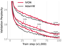
(a) GPT-2 on OpenWebText

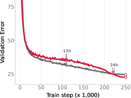
(b) ResNet-50 on ImageNet

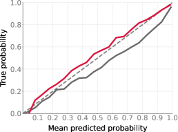
(c) Calibration on ImageNet

Figure 1: First two panels show that IVON closely matches the trajectory of AdamW (Loshchilov & Hutter, 2017) for training GPT-2 on OpenWebText and ResNet-50 on ImageNet. The computational costs of IVON and AdamW are nearly identical. Runtime in hours (h) is indicated by the arrows. The third panel shows that the predictions are also better calibrated as the red curve is closer to diagonal. Comparisons to SGD on ImageNet are in Table 1. Final numbers for IVON vs AdamW are as follows: 12.6 vs. 13.0 perplexity (lower is better) on GPT-2 (773M), 14.1 vs 14.5 perplexity on GPT-2 (355M), 17.9 vs 18.1 perplexity on GPT-2 (125M), 77.5 vs 75.2 accuracy and 0.022 vs 0.066 ECE (lower is better) on ResNet-50.

2 Challenges of Variational Learning for Large Deep Networks

Variational learning is challenging for large networks due to fundamental differences in its objective to those commonly used in deep learning. Deep learning methods estimate network weights $\bm{\theta}\in^{P}$ by minimizing empirical risk $\bar{\ell}(\bm{\theta})=\sum_{i=1}^{N}\ell_{i}(\bm{\theta})/N$, which is an average over individual losses $\ell_{i}(\bm{\theta})$ for $N$ examples. In contrast, variational methods estimate a distribution $q(\bm{\theta})$ over weights by minimizing

$$\mathcal{L}(q)=\lambda\mathbb{E}_{q(\bm{\theta})}\left[\bar{\ell}(\bm{\theta})\right]+\mathbb{D}_{\operatorname{KL}}{}\left(q(\bm{\theta})\,\|\,p(\bm{\theta})\right){},$$ (1)

where $p(\bm{\theta})$ is the prior, $\mathbb{D}_{\operatorname{KL}}{}\left(\cdot\,\|\,\cdot\right){}$ the Kullback-Leibler divergence and $\lambda$ a scaling parameter often set to $N$, but other values are useful, for example, to handle model misspecification. The objective in Eq. 1 coincides with variational inference when $\bar{\ell}(\bm{\theta})$ is a proper likelihood. We use the term variational learning to denote the general case.

Optimization of $\mathcal{L}(q)$ is fundamentally different from that of $\bar{\ell}(\bm{\theta})$. For instance, the number of parameters of $q$ can be much larger than the size of $\bm{\theta}$, making the problem harder. The number of parameters of $q$ is doubled for a diagonal-covariance Gaussian $q(\bm{\theta})=\mbox{${\cal N}$}(\bm{\theta}\,|\,\mbox{$\mbox{$\mathbf{m}$}$},\operatorname{diag}(\mbox{$\mbox{$\bm{\sigma}$}$})^{2})$ due to the estimation of two vectors of mean $\mbox{$\mbox{$\mathbf{m}$}$}\in\smash{{}^{P}}$ and standard deviation $\mbox{$\mbox{$\bm{\sigma}$}$}\in\smash{{}^{P}}$, respectively. The optimization is further complicated because of the expectation in Eq. 1, which adds additional noise during the optimization.

Due to these differences, a direct optimization of Eq. 1 remains challenging. The standard approach is to optimize it by using a standard deep learning method, say, SGD,

$$\mbox{$\mbox{$\mathbf{m}$}$}\leftarrow\mbox{$\mbox{$\mathbf{m}$}$}-\rho\widehat{\nabla}_{\text{\mbox{$\mbox{$\mathbf{m}$}$}}}\mathcal{L}\qquad\mbox{$\mbox{$\bm{\sigma}$}$}\leftarrow\mbox{$\mbox{$\bm{\sigma}$}$}-\rho\widehat{\nabla}_{\text{\mbox{$\mbox{$\bm{\sigma}$}$}}}\mathcal{L},$$

where $\rho>0$ is the learning rate. This showed promising results in early attempts of variational deep learning with several different stochastic gradient estimators $\widehat{\nabla}$ (Graves, 2011; Blundell et al., 2015). Unfortunately, these methods have been unable to keep up with the growth in scale of deep learning. The lack of progress has been attributed to various causes, such as high-variance in stochastic gradients (Kingma et al., 2015; Wen et al., 2018), issues with the temperature parameter (Wenzel et al., 2020; Noci et al., 2021), and lack of a good prior (Fortuin et al., 2022). Multiple thereotical studies have raised doubts whether variational learning can ever work at all (Trippe & Turner, 2017; Foong et al., 2020; Coker et al., 2022). Altogether, these have led to a belief that there exists an inherent trade-off between accuracy and uncertainty in Bayesian learning.

Progress in variational learning has been made on a different front by using natural-gradient methods (Sato, 2001; Hoffman et al., 2013; Khan & Lin, 2017) which have shown promising results on ImageNet (Osawa et al., 2019). Their updates resemble an Adam-like form which makes it easy to tune them at large scale. Yet, the implementation can be tricky and the cost can be much higher than Adam. For example, Osawa et al. (2019) build upon the Variational Online Newton (VON) method of Khan et al. (2018) where they replace the Hessian computation by a Gauss-Newton estimate. They implement the following Adam-like update:

$$\begin{split}\widehat{\mbox{$\mbox{$\mathbf{h}$}$}}&\leftarrow\frac{1}{|\mathcal{B}|}\sum_{i\in\mathcal{B}}\nabla\ell_{i}(\bm{\theta})^{2},\quad\text{ where }\bm{\theta}\sim q,\\ \mbox{$\mbox{$\mathbf{g}$}$}&\leftarrow\beta_{1}\mbox{$\mbox{$\mathbf{g}$}$}+\widehat{\nabla}\bar{\ell}(\bm{\theta})+s_{0}\mbox{$\mbox{$\mathbf{m}$}$}/\lambda,\\ \mbox{$\mbox{$\mathbf{h}$}$}&\leftarrow\beta_{2}\mbox{$\mbox{$\mathbf{h}$}$}+(1-\beta_{2})\widehat{\mbox{$\mbox{$\mathbf{h}$}$}},\\ \mbox{$\mbox{$\mathbf{m}$}$}&\leftarrow\mbox{$\mbox{$\mathbf{m}$}$}-\alpha_{t}\mbox{$\mbox{$\mathbf{g}$}$}/(\mbox{$\mbox{$\mathbf{h}$}$}+c),\\ \mbox{$\mbox{$\bm{\sigma}$}$}&\leftarrow 1/\sqrt{\lambda(\mbox{$\mbox{$\mathbf{h}$}$}+c)}.\end{split}$$ (2)

Here, a prior $p(\bm{\theta})=\mbox{${\cal N}$}(\bm{\theta}\,|\,0,\mathbf{I}/s_{0})$ is used. The difficult computation is in the first line of Eq. 2 where a Gauss-Newton estimate over a minibatch $\mathcal{B}$ is computed at a sample from the Gaussian, while the rest is similar to Adam: the second line is gradient momentum, where $s_{0}\mbox{$\mbox{$\mathbf{m}$}$}/\lambda$ is added due to the prior. The third and fourth line are identical to the scale and parameter vectors updates, respectively. The constant $c=\gamma+s_{0}/\lambda$ where $\gamma>0$ is a damping parameter.

The computation of the Gauss-Newton estimate is tricky because it requires per-example squaring, which is not a standard operation in deep learning and could be difficult to implement. In Osawa et al. (2019, Fig. 1), this ends up increasing the cost by a factor of two. The Gauss-Newton estimate also introduces an additional approximation in the variational learning, even though it helps to ensure the positivity of $\mathbf{h}$. Another issue is the use of an additional damping parameter $\gamma$ which departs from the Bayesian framework.

Ideally, we want a method that directly optimizes Eq. 1 without additional approximations and also seamlessly fits into an Adam-like framework without any significant computational overheads. Methods such as MC-dropout, SWAG, and Laplace do not solve this problem, and rather circumvent it by relying on algorithms that optimize $\bar{\ell}$, not $\mathcal{L}$. The goal of this paper is to propose a method that can match the accuracy of Adam while directly optimizing $\mathcal{L}$.

3 Improved Variational Online Newton

We present the Improved Variational Online Newton (IVON) method by adapting the method of Lin et al. (2020) and introducing practical tricks necessary to achieve good performance at large scale. They propose an improved version of the Bayesian Learning Rule (Khan & Rue, 2021) which ensures positivity of certain variational parameters, such as, the Gaussian variance or scale parameter of Gamma distribution. For the Gaussian case, they propose an Adam-like update which makes the update in Eq. 2 simpler. Specifically, they use the following Hessian estimate by using the reparameterization trick,

$$\widehat{\mbox{$\mbox{$\mathbf{h}$}$}}\leftarrow\widehat{\nabla}\bar{\ell}(\bm{\theta})\cdot\frac{\bm{\theta}-\mbox{$\mbox{$\mathbf{m}$}$}}{\mbox{$\mbox{$\bm{\sigma}$}$}^{2}},$$ (3)

which does not require per-example gradient squares, rather just a single vector multiplication with the minibatch gradient. The above estimate is easy to compute but, unlike the Gauss-Newton estimate, it is not always positive and can make $\mathbf{h}$ in Eq. 2 negative (Khan et al., 2018, App. D). Lin et al. (2020) solve this problem by using Riemannian gradient descent which ensures positivity by adding an extra term in the update of $\mathbf{h}$,

$$\mbox{$\mbox{$\mathbf{h}$}$}\leftarrow(1-\rho)\mbox{$\mbox{$\mathbf{h}$}$}+\rho\widehat{\mbox{$\mbox{$\mathbf{h}$}$}}+\mbox{$\frac{1}{2}$}\rho^{2}(\mbox{$\mbox{$\mathbf{h}$}$}-\widehat{\mbox{$\mbox{$\mathbf{h}$}$}})^{2}/(\mbox{$\mbox{$\mathbf{h}$}$}+s_{0}/\lambda).$$ (4)

Positivity holds even when $\widehat{\mbox{$\mbox{$\mathbf{h}$}$}}$ are negative, as shown in Lin et al. (2020, Theorem 1).

In Alg. 1, we use the two modifications (highlighted in red) to get an improved version of VON, called IVON. The updates closely resemble Adam. One major change is the sampling step in line 2 and a minor difference is the lack of square-root over $\mbox{$\mbox{$\mathbf{h}$}$}+\delta$ in line 7. IVON therefore uses a proper Newton-like update but, instead of using $\widehat{\mbox{$\mbox{$\mathbf{h}$}$}}$, it uses the smoothed average $\mathbf{h}$. This can reduce instability due to the noise in the Hessian estimate. The Hessian estimator in Eq. 3 is also less costly compared to other second-order optimizers (Dauphin et al., 2015; Yao et al., 2021; Liu et al., 2023). It is valid even for losses that are not twice-differentiable (for example, for ReLU activations). These aspects make IVON a unique second-order optimizer with nearly identical cost to Adam.

Algorithm 1 Improved Variational Online Newton (IVON). Hyperparameter setting is described in App. A.

0:  Learning rates $\{\alpha_{t}\}$, weight-decay $\delta>0$.

0:  Momentum parameters $\beta_{1},\beta_{2}\in[0,1)$.

0:  Hessian init $h_{0}>0$.

0:  $\mbox{$\mbox{$\mathbf{m}$}$}\leftarrow\text{(NN-weights)}$,   $\mbox{$\mbox{$\mathbf{h}$}$}\leftarrow h_{0}$,    $\mbox{$\mbox{$\mathbf{g}$}$}\leftarrow 0$,    $\lambda\leftarrow N$.

0:  $\mbox{$\mbox{$\bm{\sigma}$}$}\leftarrow 1/\sqrt{\lambda(\mbox{$\mbox{$\mathbf{h}$}$}+\delta)}$.

0:  $\alpha_{t}\leftarrow(h_{0}+\delta)\alpha_{t}$  for all $t$.

1:  for $t=1,2,\ldots$ do

2:     $\widehat{}\mbox{$\mbox{$\mathbf{g}$}$}\leftarrow{\widehat{\nabla}}\bar{\ell}(\bm{\theta})$, where $\color[rgb]{1,0,0}\bm{\theta}\sim q$

3:     $\widehat{}\mbox{$\mbox{$\mathbf{h}$}$}\leftarrow{\color[rgb]{1,0,0}\widehat{}\mbox{$\mbox{$\mathbf{g}$}$}\cdot(\bm{\theta}-\mbox{$\mbox{$\mathbf{m}$}$})/\mbox{$\mbox{$\bm{\sigma}$}$}^{2}}$

4:     $\mbox{$\mbox{$\mathbf{g}$}$}\leftarrow\beta_{1}\mbox{$\mbox{$\mathbf{g}$}$}+(1-\beta_{1})\widehat{}\mbox{$\mbox{$\mathbf{g}$}$}$

5:     $\mbox{$\mbox{$\mathbf{h}$}$}\leftarrow\beta_{2}\mbox{$\mbox{$\mathbf{h}$}$}+(1-\beta_{2})\widehat{}\mbox{$\mbox{$\mathbf{h}$}$}$${\color[rgb]{1,0,0}+\mbox{$\frac{1}{2}$}(1-\beta_{2})^{2}(\mbox{$\mbox{$\mathbf{h}$}$}-\widehat{}\mbox{$\mbox{$\mathbf{h}$}$})^{2}/(\mbox{$\mbox{$\mathbf{h}$}$}+\delta)}$

6:     $\bar{}\mbox{$\mbox{$\mathbf{g}$}$}\leftarrow\mbox{$\mbox{$\mathbf{g}$}$}/(1-\beta_{1}^{t})$

7:     $\mbox{$\mbox{$\mathbf{m}$}$}\leftarrow\mbox{$\mbox{$\mathbf{m}$}$}-\alpha_{t}(\bar{}\mbox{$\mbox{$\mathbf{g}$}$}+\delta\mbox{$\mbox{$\mathbf{m}$}$})/(\mbox{$\mbox{$\mathbf{h}$}$}+\delta)$

8:     $\mbox{$\mbox{$\bm{\sigma}$}$}\leftarrow 1/\sqrt{\lambda(\mbox{$\mbox{$\mathbf{h}$}$}+\delta)}$

9:  end for

10:  return $\mbox{$\mbox{$\mathbf{m}$}$},\mbox{$\mbox{$\bm{\sigma}$}$}$

Dataset / Model	Method		Top-1 Acc. $\uparrow$	Top-5 Acc. $\uparrow$	NLL $\downarrow$	ECE $\downarrow$	Brier $\downarrow$
	AdamW		($2\%$) $75.16_{\pm 0.14}$	$92.37_{\pm 0.03}$	$1.018_{\pm 0.003}$	$0.066_{\pm 0.002}$	$0.349_{\pm 0.002}$
	SGD		($1\%$) $76.63_{\pm 0.45}$	$93.21_{\pm 0.25}$	$0.917_{\pm 0.026}$	$0.038_{\pm 0.009}$	$0.326_{\pm 0.006}$
	IVON@mean		$77.30_{\pm 0.08}$	$93.58_{\pm 0.05}$	$0.884_{\pm 0.002}$	$0.035_{\pm 0.002}$	${\bf 0.316}_{\pm 0.001}$
ImageNet ResNet-50 (26M params)	IVON		${\bf 77.46}_{\pm 0.07}$	${\bf 93.68}_{\pm 0.04}$	${\bf 0.869}_{\pm 0.002}$	${\bf 0.022}_{\pm 0.002}$	${\bf 0.315}_{\pm 0.001}$
	AdamW		($15\%$) $47.33_{\pm 0.90}$	$71.54_{\pm 0.95}$	$6.823_{\pm 0.235}$	$0.421_{\pm 0.008}$	$0.913_{\pm 0.018}$
	SGD		($1\%$) $61.39_{\pm 0.18}$	$82.30_{\pm 0.22}$	$1.811_{\pm 0.010}$	$0.138_{\pm 0.002}$	$0.536_{\pm 0.002}$
	IVON@mean		${\bf 62.41}_{\pm 0.15}$	${\bf 83.77}_{\pm 0.18}$	$1.776_{\pm 0.018}$	$0.150_{\pm 0.005}$	$0.532_{\pm 0.002}$
TinyImageNet ResNet-18 (11M params)	IVON		${\bf 62.68}_{\pm 0.16}$	${\bf 84.12}_{\pm 0.24}$	${\bf 1.528}_{\pm 0.010}$	${\bf 0.019}_{\pm 0.004}$	${\bf 0.491}_{\pm 0.001}$
	AdamW		($11\%$) $\smash{50.65_{\pm 0.0^{\ast}}}$	$\smash{74.94_{\pm 0.0^{\ast}}}$	$\smash{4.487_{\pm 0.0^{\ast}}}$	$\smash{0.357_{\pm 0.0^{\ast}}}$	$\smash{0.812_{\pm 0.0^{\ast}}}$
	SGD		($2\%$) $59.39_{\pm 0.50}$	$81.34_{\pm 0.30}$	$2.040_{\pm 0.040}$	$0.176_{\pm 0.006}$	$0.577_{\pm 0.007}$
	IVON@mean		${\bf 60.85}_{\pm 0.39}$	${\bf 83.89}_{\pm 0.14}$	$1.584_{\pm 0.009}$	$0.053_{\pm 0.002}$	${\bf 0.514}_{\pm 0.003}$
TinyImageNet PreResNet-110 (4M params)	IVON		${\bf 61.25}_{\pm 0.48}$	${\bf 84.13}_{\pm 0.17}$	${\bf 1.550}_{\pm 0.009}$	${\bf 0.049}_{\pm 0.002}$	${\bf 0.511}_{\pm 0.003}$
	AdamW		($11\%$) $64.12_{\pm 0.43}$	$86.85_{\pm 0.51}$	$3.357_{\pm 0.071}$	$0.278_{\pm 0.005}$	$0.615_{\pm 0.008}$
	SGD		($1\%$) $74.46_{\pm 0.17}$	$92.66_{\pm 0.06}$	$1.083_{\pm 0.007}$	$0.113_{\pm 0.001}$	$0.376_{\pm 0.001}$
	IVON@mean		$74.51_{\pm 0.24}$	$92.74_{\pm 0.19}$	$1.284_{\pm 0.013}$	$0.152_{\pm 0.003}$	$0.399_{\pm 0.002}$
CIFAR-100 ResNet-18 (11M params)	IVON		${\bf 75.14}_{\pm 0.34}$	${\bf 93.30}_{\pm 0.19}$	${\bf 0.912}_{\pm 0.009}$	${\bf 0.021}_{\pm 0.003}$	${\bf 0.344}_{\pm 0.003}$
	AdamW		($10\%$) $65.88_{\pm 0.84}$	$88.34_{\pm 0.56}$	$2.893_{\pm 0.088}$	$0.258_{\pm 0.006}$	$0.578_{\pm 0.014}$
	SGD		($2\%$) $74.19_{\pm 0.11}$	$92.41_{\pm 0.14}$	$1.204_{\pm 0.012}$	$0.137_{\pm 0.002}$	$0.393_{\pm 0.004}$
	IVON@mean		$75.23_{\pm 0.23}$	$93.45_{\pm 0.16}$	$1.149_{\pm 0.010}$	$0.136_{\pm 0.002}$	$0.380_{\pm 0.003}$
CIFAR-100 PreResNet-110 (4M params)	IVON		${\bf 75.81}_{\pm 0.18}$	${\bf 93.93}_{\pm 0.19}$	${\bf 0.884}_{\pm 0.007}$	${\bf 0.030}_{\pm 0.003}$	${\bf 0.336}_{\pm 0.001}$

Table 1: IVON improves both accuracy and uncertainty over SGD and AdamW. Improvements in accuracy by IVON are shown in red. The performance of AdamW is not good on the smaller datasets likely due to overfitting when training for $200$ epochs. IVON does not have this issue. Additional results are in the appendix in Tables 8, 9 and 10 and Table 12.

Below, we list a few practical tricks needed for good results.

1. Instead of the prior precision $s_{0}$, we use the weight-decay regularizer $\delta$ as the prior. The scaling parameter $\lambda$ is set to $N$, except for finetuning on small datasets.

2. Unlike Lin et al. (2020, Fig. 1), the update of $\mathbf{h}$ does not use $\delta$. We also update $\mathbf{h}$ before $\mathbf{m}$ which has no impact on the performance. Also, we do not debias $\mathbf{h}$.

3. The Hessian $\mathbf{h}$ is initialized with a constant $h_{0}$. Lin et al. (2020) most likely set it to 0 due to the debiasing step used in their work. We find the initialization to be useful. Too small values can destabilize the training while larger values may give poor performance.

4. When training transformers, it can be helpful to clip the preconditioned gradient in line 7 entrywise to $[-\xi,\xi]$.

5. Optionally, we rescale $\alpha_{t}$ by $(h_{0}+\delta)$ so that the first steps of the algorithm have step-size close to the initial $\alpha_{t}$. When clipping is used, this step is omitted.

Momentum $\beta_{1}$, learning rate $\alpha_{t}$ and weight-decay $\delta$ can be set in the same fashion as for standard optimizers, as well as minibatch size and clipping radius $\xi$. $\beta_{2}$ typically needs to be closer to one as in Adam, for instance, values of $\beta_{2}=0.99995$ work well. Setting of $h_{0}$ and $\lambda$ is also easy, as discussed above. This makes obtaining good results with IVON often very easy. A detailed guide for hyperparameter setting is in App. A.

We implement IVON as a drop-in replacement for Adam in PyTorch, where only two lines need to be added (shown in red below) to sample noisy weights. for inputs, targets in dataloader:  for _ in range(num_mc_samples):   with optimizer.sampled_params(train=True):    optimizer.zero_grad()    outputs = model(inputs)    loss = loss_fn(outputs, targets)    loss.backward()  optimizer.step() IVON training can easily be generalized to using multiple MC samples. Furthermore, is is easliy parallelized, for example, by using multiple GPUs. On the other hand, memory-efficiency can be improved by using accumulation steps for the gradient and Hessian estimate on each device. This can be implemented by replacing the calculations of $\widehat{\mbox{$\mbox{$\mathbf{g}$}$}}$ and $\widehat{\mbox{$\mbox{$\mathbf{h}$}$}}$ in line 2 and 3 of Alg. 1, respectively, by the following quantities:

$$\widehat{}\mbox{$\mbox{$\mathbf{g}$}$}=\sum_{j,s}\alpha_{j}\widehat{\nabla}\bar{\ell}(\bm{\theta}_{j}^{(s)}),~{}~{}\widehat{}\mbox{$\mbox{$\mathbf{h}$}$}=\sum_{j,s}\alpha_{j}\widehat{\nabla}\bar{\ell}(\bm{\theta}_{j}^{(s)})\frac{\bm{\theta}_{j}^{(s)}-\mbox{$\mbox{$\mathbf{m}$}$}}{\mbox{$\mbox{$\bm{\sigma}$}$}^{2}}.$$

Here, we use a different random weight $\bm{\theta}_{j}^{(s)}\sim q$ on each device and accumulation step, where the index $j$ ranges over number of devices times accumulation steps and the index $s$ over the number of per-device MC samples $S$. Using a different random noise is similar to the local reparametrization trick by Kingma et al. (2015) which leads to reduced variance. The weighting coefficients are given by $\alpha_{j}=B_{j}/\sum_{j}SB_{j}$ where $B_{j}$ denotes the minibatch-size of the stochastic gradient $\widehat{\nabla}\bar{\ell}$ in device/accumulation step $j$.

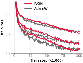
(a) Training loss on OpenWebText

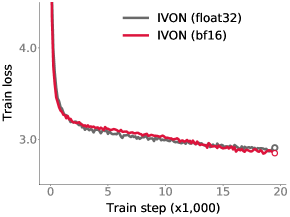
(b) Low precision training

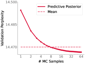
(c) Predictive posterior

Figure 2: When training GPT-2, IVON not only improves upon AdamW in terms of validation perplexity but also converges to matching or even better training loss than AdamW, as shown in (a). IVON also provides stable training when using low-precision floating point numbers, as shown in (b) on the example of bf16. Finally, in (c) we see that using posterior averaging using IVON’s learned distribution we can further improve the validation perplexity on GPT-2.

4 IVON is Effective for Large Deep Networks

We show that IVON effectively trains large deep networks from scratch (Sec. 4.1) and enables many downstream applications, such as, predictive uncertainty (Sec. 4.2), finetuning and model merging (Sec. 4.3), as well as predicting generalization and finding influential training examples (Sec. 4.4). We perform ablation studies on computational efficiency (Sec. B.1) and the choice of Hessian estimator (Sec. B.2) In the following, we refer by IVON@mean to the prediction using $\mathbf{m}$ as the weights, whereas IVON denotes a model average with $64$ samples drawn from the posterior learned by IVON.

4.1 Better Scalability and Generalization

Here, we show how IVON scalably trains large models from scratch. First, we train LLMs with up to $773$M parameters from scratch on ca. $50$B tokens in Sec. 4.1.1. Then, we show improved accuracy and uncertainty when training various image classification models, such as ResNets with 26M parameters at ImageNet-scale, in Sec. 4.1.2. Additional results on smaller recurrent neural networks with 2M parameters are shown in Sec. D.1.

4.1.1 Pretraining language models

Pretraining transformer language models (Vaswani et al., 2017) with variational learning has been challenging and no large-scale result exists so far. We show that IVON can train large language models at scale. We train models following the GPT-2 (Radford et al., 2019) architecture for $49.2$ billion tokens in total on the OpenWebText corpus (Gokaslan & Cohen, 2019). We use the same hyperparameters for AdamW as prior work (Liu et al., 2023) and optimize the hyperparameters for IVON by grid search on a smaller model. We pretrain models with $125$M, $355$M (“GPT-2-medium”), and $773$M (“GPT-2-large”) parameters from scratch using gradient clipping to stabilize the training. Details and exact hyperparameters are given in Sec. C.1.

Validation perplexities are reduced from $18.1$ to $17.9$, from $14.5$ to $14.1$ and from $13.0$ to $12.6$ for models with 125M, 355M and 773M parameters, respectively, as shown in Fig. 1(a). IVON also converges to matching or even better training loss than AdamW, as shown in Fig. 2(a). In Fig. 2(b) we show that IVON also provides stable training with bf16 precision, and in Fig. 2(c) we show that using the predictive posterior by sampling multiple models from IVON’s learned distribution further improves performance when a sufficient number of samples is used. This demonstrates that variational learning is effective for training large Transformers from scratch on large datasets.

4.1.2 Image classification

We compare IVON to AdamW (Loshchilov & Hutter, 2017) and SGD for image classification on various models and benchmarks. Table 1 shows that IVON improves upon both AdamW and the stronger SGD baseline in terms of both accuracy and uncertainty, here measured by negative log-likelihood (NLL), expected calibration error (ECE), and Brier score. We also find that IVON does not overfit on smaller tasks, unlike AdamW which tends to overfit on TinyImageNet and CIFAR-100. This holds on various datasets and models trained for $200$ epochs, of which we show here: 1) ResNet-50 with $\approx 25.6$M parameters (He et al., 2016a) on ImageNet-1k which has $\approx 1.2$M images with $1000$ classes; 2) ResNet-18 with 11M parameters and PreResNet-110 with $4$M parameters on both TinyImageNet and CIFAR-100. We list further details on the experiments in Sec. C.2 along with more results using also DenseNet-121 and ResNet-20 on other datasets, such as CIFAR-10. There, IVON again improves accuracy and uncertainty.

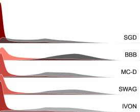
(a) CIFAR-10 & SVHN (OOD)

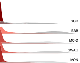
(b) CIFAR-10 & Flowers102 (OOD)

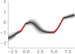
(c) IVON in-between uncertainty

Figure 3: In panel (a) and (b) we see that IVON’s histogram of predictive entropy has a high peak similar to SGD for in-domain data (red, CIFAR-10) but at the same time is spread out widely similar to the other Bayesian deep learning methods for out-of-domain data (gray, SVHN (a) & Flowers102 (b)). The colors are shaded proportional to the height of the peak, that is, darker red or darker gray indicates a higher peak. In panel (c) we see that IVON handles in-between uncertainty well, which has been shown to be challenging for variational methods by Foong et al. (2019).

We hypothesize that these improvements are partly due to flat-minima seeking properties of variational learning. Methods aimed to find flat minima, such as sharpness-aware minimization (SAM) (Foret et al., 2021), have recently gained in popularity to boost test-accuracy. Möllenhoff & Khan (2023) have shown that SAM optimizes a relaxation of the variational loss in Eq. 1. Our results here indicate that similar improvements can be obtained by direct optimization.

4.2 Posterior Averaging for Predictive Uncertainty

Variational learning naturally allows for improved predictive uncertainties, because Monte-Carlo samples from the learned posterior can be averaged to estimate the predictive posterior. Unlike other BDL methods, no postprocessing or model architecture changes are required for this. In the following, we compare IVON to Bayes-by-Backprop (BBB), MC Dropout, SWAG and deep ensembles (Lakshminarayanan et al., 2017) in in-domain and out-of-domain (OOD) settings. We report common metrics from existing benchmarks (Liang et al., 2018; Snoek et al., 2019). Further details on the experimental setup can be found in Sec. C.3.

	Acc. (%) $\uparrow$	NLL $\downarrow$	ECE $\downarrow$	Brier $\downarrow$
AdamW	$90.04_{\pm 0.27}$	$0.589_{\pm 0.018}$	$0.074_{\pm 0.002}$	$0.170_{\pm 0.004}$
SGD	$91.86_{\pm 0.14}$	$0.288_{\pm 0.015}$	$0.040_{\pm 0.004}$	$0.126_{\pm 0.004}$
BBB	$91.09_{\pm 0.16}$	$0.289_{\pm 0.005}$	$0.053_{\pm 0.001}$	$0.139_{\pm 0.002}$
MC-D	$91.85_{\pm 0.17}$	$0.242_{\pm 0.004}$	${\bf 0.008}_{\pm 0.002}$	$0.120_{\pm 0.002}$
SWAG	$92.45_{\pm 0.23}$	$0.230_{\pm 0.002}$	$0.024_{\pm 0.002}$	$0.112_{\pm 0.002}$
IVON	${\bf 92.71}_{\pm 0.07}$	${\bf 0.219}_{\pm 0.002}$	${\bf 0.008}_{\pm 0.001}$	${\bf 0.108}_{\pm 0.001}$
Deep Ens.	$93.57_{\pm 0.16}$	$0.198_{\pm 0.003}$	${\bf 0.014}_{\pm 0.001}$	$0.096_{\pm 0.001}$
Multi-IVON	${\bf 94.37}_{\pm 0.13}$	${\bf 0.179}_{\pm 0.002}$	$0.029_{\pm 0.001}$	${\bf 0.087}_{\pm 0.001}$

Table 2: IVON’s predictive uncertainty is better than other baselines for in-domain examples. Multi-IVON is a mixture-of-Gaussian ensemble which further improves the performance and is competitive with a deep ensemble.

4.2.1 In-domain comparison

To evaluate in-domain uncertainty, we train and evaluate ResNet-20 models (He et al., 2016a) on the smaller CIFAR-10 dataset for a fair comparison, because BBB is difficult to apply successfully on larger datasets. Results are reported in Table 2. Overall, all BDL baselines except for BBB, which is known to under-perform, have significantly better uncertainty metrics than SGD. Among all non-ensemble approaches, IVON stands out in both accuracy and uncertainty estimation.

Deep ensembles made up of five models from different SGD runs, on the other hand, clearly improve over the non-ensemble methods. This said, ensembling is a generic technique that can be seen as a mixture with equal importance and IVON is easily amenable to such posterior forms (Lin et al., 2019). Therefore, we evaluate a mixture-of-Gaussian posterior constructed from five independently-trained IVON models, referred to as Multi-IVON in Table 2. We find that this can further improve upon deep ensembles. This confirms that good in-domain uncertainty estimates can be obtained using variational learning with IVON.

	FPR@95% $\downarrow$	Det. Err. $\downarrow$	AUROC $\uparrow$	AUPR-In $\uparrow$	AUPR-Out $\uparrow$
SVHN, see Fig. 3(a)
SGD	$20.7_{\pm 1.6}$	$18.8_{\pm 0.9}$	$86.7_{\pm 1.0}$	$81.8_{\pm 1.4}$	$91.8_{\pm 0.7}$
BBB	$24.5_{\pm 0.7}$	$17.8_{\pm 0.3}$	$87.0_{\pm 0.3}$	$83.4_{\pm 0.4}$	$91.3_{\pm 0.4}$
MC-D	$20.7_{\pm 1.3}$	${\bf 17.0}_{\pm 0.6}$	$88.0_{\pm 0.8}$	$84.6_{\pm 0.9}$	$92.1_{\pm 0.7}$
SWAG	$19.8_{\pm 2.2}$	${\bf 16.6}_{\pm 1.0}$	${\bf 88.9}_{\pm 1.1}$	${\bf 85.3}_{\pm 1.2}$	$93.0_{\pm 0.9}$
IVON	${\bf 17.4}_{\pm 0.8}$	${\bf 16.6}_{\pm 0.5}$	${\bf 89.2}_{\pm 0.4}$	${\bf 85.2}_{\pm 0.6}$	${\bf 93.4}_{\pm 0.4}$
Flowers102, see Fig. 3(b)
SGD	$22.1_{\pm 0.5}$	$20.7_{\pm 0.4}$	$86.3_{\pm 0.3}$	$92.1_{\pm 0.2}$	$75.4_{\pm 0.4}$
BBB	$22.2_{\pm 0.8}$	$19.5_{\pm 0.7}$	$88.2_{\pm 0.7}$	$93.1_{\pm 0.5}$	$79.8_{\pm 0.9}$
MC-D	$20.3_{\pm 0.8}$	$19.6_{\pm 1.1}$	$87.8_{\pm 0.9}$	$93.0_{\pm 0.7}$	$78.4_{\pm 1.1}$
SWAG	$19.5_{\pm 0.8}$	${\bf 18.1}_{\pm 0.5}$	${\bf 89.3}_{\pm 0.6}$	${\bf 93.9}_{\pm 0.4}$	${\bf 81.0}_{\pm 0.9}$
IVON	${\bf 17.8}_{\pm 0.5}$	${\bf 18.1}_{\pm 0.5}$	${\bf 89.0}_{\pm 0.5}$	${\bf 93.8}_{\pm 0.3}$	${\bf 80.2}_{\pm 0.8}$

Table 3: IVON improves OOD detection, here for ResNet-20/CIFAR-10 evaluated on SVHN and Flowers102.

4.2.2 Out-of-domain experiments

Next, we consider the OOD case by reusing the CIFAR-10 models on data from a different domain. While we would expect the model to be certain for correct in-domain predictions, it should be uncertain for out-of-domain examples. This would allow for distinguishing the CIFAR-10 data from OOD samples, for which we use the street view house number (SVHN) (Netzer et al., 2011) and the 102 Flowers dataset (Nilsback & Zisserman, 2008, Flowers102).

Table 3 shows that IVON is consistently the best at distinguishing OOD examples from SVHN and Flowers102 from in-domain CIFAR-10 data. These results are further illustrated by the predictive entropy plots in Figs. 3(a) and 3(b). In these plots, IVON’s histogram has a similarly high peak as SGD for in-domain data (red), but is much more spread out than SGD for out-of-domain data (gray). While the other Bayesian deep learning method’s histograms are also spread out for OOD data, they struggle to achieve a high peak for in-domain data. Overall, IVON’s histogram has the most clear separation between in-domain data and out-of-domain data. As illustrated in Fig. 3(c), IVON’s predictive posterior also gives good in-between uncertainty which has been challenging for other variational methods (Foong et al., 2019). We show further distribution shift experiments in Sec. D.2.

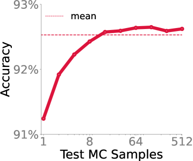
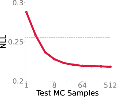
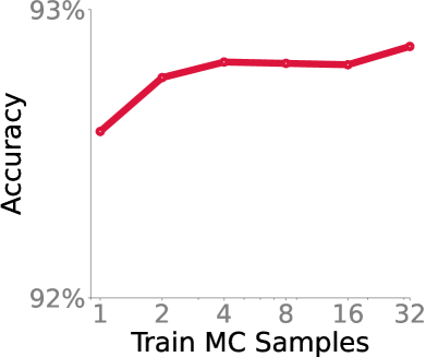
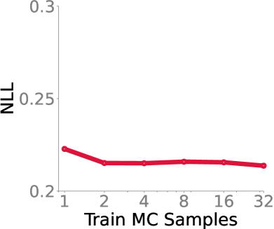
Figure 4: Using more MC samples during inference (top row) or training (bottow row) can improve both accuracy and NLL, here plotted for ResNet-20 on CIFAR-10.

4.2.3 MC samples for averaging

Here, we summarize results for using an increasing number of MC samples for prediction with ResNet-20 on CIFAR-10. We find consistent improvements when using more MC samples both during training and inference, but eventually improvements saturate and deliver diminishing returns. Fig. 4 shows that using multiple samples during inference also improves over using the learned mean, especially in terms of NLL, but at higher inference cost. Similarly, using multiple samples during training improves both accuracy and uncertainty, as highlighted in Fig. 4.

4.2.4 NeurIPS 2021 Competition

An earlier version of IVON won first place in both tracks of the NeurIPS 2021 competition on approximate inference in Bayesian deep learning (Wilson et al., 2022). The methods were evaluated by their difference in predictions to these of a ’ground-truth’ posterior computed on hundreds of TPUs. The winning solution used Multi-IVON (see also Table 2), that is, a uniformly weighted mixture-of-Gaussian posterior constructed from independent runs of IVON. We summarize the results of the challenge and the differences of the earlier version to Alg. 1 in Sec. D.3.

4.3 Finetuning and Model Merging

The variance of IVON’s model posterior provides valuable information for adaptation, since it shows how far parameters can be varied without a sharp loss increase. The natural-gradient descent update of IVON also preconditions the mean update with the posterior variance, encouraging adaptation in directions without large loss increase. Furthermore, we expect the variance to be useful for uncertainty-guided model merging (Daheim et al., 2024), because it can be used to scale models when merging. The following experiments confirm this and show improvements for both applications.

4.3.1 Finetuning pretrained language models

	MNLI	QNLI	QQP	RTE	SST2	MRPC	CoLA	STS-B
RoBERTa (125M params)
AdamW	87.7	92.8	90.9	80.9	94.8	85.8	63.6	90.6
IVON@mean	87.8	92.6	90.8	80.6	95.0	87.3	63.3	90.8
DeBERTAv3 (440M params)
AdamW	91.3	95.7	93.1	91.0	96.5	91.0	74.8	92.4
IVON@mean	91.6	95.7	93.0	91.7	96.9	91.9	75.1	92.6
AdamW†	91.8	96.0	93.0	92.7	96.9	92.2	75.3	93.0

Table 4: In our experiments, IVON also gives improvements over AdamW when finetuning DeBERTAv3${}_{\text{large}}$ with 440M params and RoBERTa${}_{\text{base}}$ with 125M parameters on GLUE. Results on development set. $\dagger$ is state-of-the-art taken from He et al. (2023).

We compare finetuning a large masked-language model DeBERTAv3 (He et al., 2023) using AdamW and IVON on GLUE (Wang et al., 2018), excluding WNLI following prior work (Devlin et al., 2019). DeBERTAv3 has 440M parameters and we finetune the full model using a publicly available checkpoint that was initially trained with AdamW. Table 4 shows that IVON can improve upon AdamW in our experiments, both on classification and regression tasks (STS-B), even when evaluated at the learned mean. However, we also could not fully replicate the AdamW results from He et al. (2023) which show higher scores. For RoBERTa (Liu et al., 2019), we also find that IVON can give improvements over AdamW on average. Further details on the experiment and hyperparameters are shown in Sec. C.4.

	IMDB	Yelp	RT	SST2	Amazon	Avg.	Overhead
SG	93.5	97.0	89.7	92.8	96.6	93.9	100%
IVON	93.6	96.9	89.8	92.8	96.7	94.0	0%

Table 5: IVON’s weight uncertainty can be used for improved model merging without incurring any overhead, here measured by the share of one training epoch and compared to a squared gradients estimator (SG) that uses an additional pass over the data after training.

4.3.2 Merging masked-language models

We replicate the experimental set-up from Daheim et al. (2024) and merge RoBERTa models finetuned using IVON on IMDB (Maas et al., 2011), Amazon (Zhang et al., 2015), Yelp (Zhang et al., 2015), RottenTomatoes (Pang & Lee, 2005), and SST2 (Socher et al., 2013), according to the method outlined in Sec. C.5. We compare using IVON’s learned variance estimate against a squared gradient (SG) estimator as scaling matrices for model merging. The SG estimator uses $\sum_{i}[\nabla\ell(\hat{\mbox{$\mbox{$\mathbf{y}$}$}}_{i},\mbox{$\mbox{$\mathbf{x}$}$}_{i})]^{2}$ after training, where $\hat{\mbox{$\mbox{$\mathbf{y}$}$}}_{i}$ is sampled from the model distribution. This can be seen as a Laplace approximation (Daheim et al., 2024).

Table 5 shows that both estimates perform similarly. However, our variational method does not have any overhead unlike Laplace which requires an additional pass over training data and therefore incurs significant overhead. We expect even better results for IVON when the model is pretrained with it, because the variance is already estimated during pretraining. We leave this for future work.

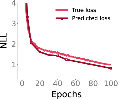
(a) IVON

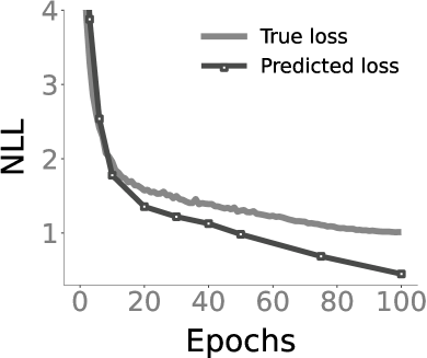
(b) AdamW

Figure 5: IVON predicts test loss much more faithfully than AdamW, where especially at the end of training the predicted loss diverges heavily from the test loss. IVON also faithfully predicts the bump in loss around epoch 40.

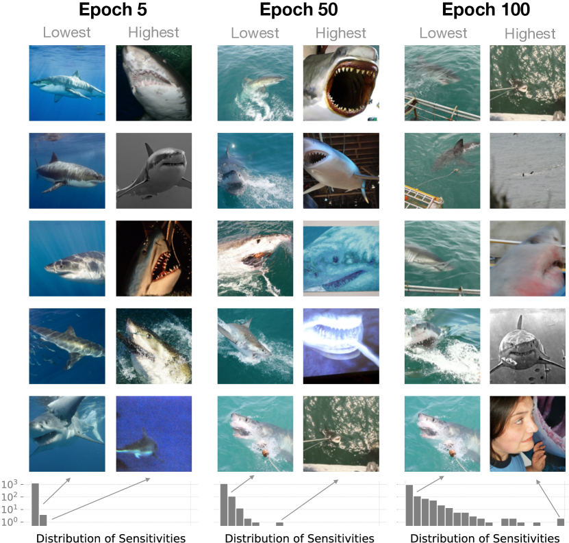
Figure 6: Sensitivity can also be used to directly analyze the data samples. At different stages of training, we show the data examples for the “great white shark” class on ImageNet with lowest and highest sensitivities, as well as the histogram of data sensitivity. As the training progress, the model becomes more sensitive to a few “unusual” data examples. This is especially apparent at the end of training, where only a few examples have high sensitivity.

4.4 Sensitivity Analysis and Predicting Generalization

The posterior can also be used to estimate a model’s sensitivity to perturbation in the training data, such as example removal, without expensive retraining. Sensitivity estimates can be used to find influential examples, clean datasets, and diagnose model training by estimating generalization performance. While existing works often rely on Hessian approximations at a converged model (Koh & Liang, 2017) or even on full retraining (Feldman & Zhang, 2020), the variational posterior can be used to estimate sensitivity already during training (Nickl et al., 2023), enabling model diagnosis on-the-fly and avoiding costly post-hoc analysis.

We discuss two applications for diagnosing models: qualitative sensitivity analysis of training examples and estimation of generalization performance without a held-out validation set. We summarize the approach and describe hyperparameters, models and datasets in Sec. C.6.

4.4.1 Prediction of model generalization

Sensitivity estimates from IVON can be used to approximate a leave-one-out (LOO) cross-validation criterion without retraining. This allows us to train a model with all available data and standard loss, while estimating generalization performance during training with the LOO objective. The estimate can be helpful, for example, to detect over-fitting or for early-stopping without a separate validation set.

In Fig. 5 we find that IVON can be used to faithfully predict the loss on unseen test data. The LOO objective is evaluated using sensitivities calculated from IVON during training. The heuristic estimate with sensitivities obtained from AdamW’s squared-gradients performs less well and diverges at the end of training. In Fig. 5(a) we notice that IVON can even predict the bump in the test-loss around epoch 40. For the plot, we use a similar ImageNet training set-up as in Table 1 and evaluate the LOO criterion at regular intervals. We show further results using different architectures on CIFAR-10 in Sec. D.4.

4.4.2 Training data sensitivity analysis

IVON’s posterior variance is useful to understand sensitivitiy to data. Possible applications are to clean the dataset from mislabeled or ambiguous training samples that are characterized by high sensitivity or for removing redundant, low-sensitivity data to speed up the training.

Fig. 6 illustrates low- and high-sensitivity images at different training stages with the same sensitivities that were used in Fig. 5 to predict generalization. All samples have small sensitivities in the first epochs and, as training progresses, the model becomes highly sensitive to only a small fraction of the examples. At the end of training the most sensitive examples are highly unusual, for instance, showing the face of a woman rather than a shark.

5 Discussion and Limitations

We show the effectiveness of variational learning for training large networks. Especially our results on GPT-2 and other LLMs are first of their kind and clearly demonstrate the potential that variational learning holds. We also discussed many new use cases where we consistently find benefits by switching to a variational approach. We expect our results to be useful for future work on showing the effectiveness of Bayesian learning in general.

Although we borrow practical tricks from deep learning, not all of them are equally useful for IVON, for example, we find that IVON does not go well with batch normalization layers (Ioffe & Szegedy, 2015). Future research should explore this limitation and investigate the reasons behind the effectiveness of some practical tricks. Using MC samples in variational learning increases the computation cost and we believe it is difficult to fix this problem. Deterministic versions of the variational objective can be used to fix this, for example, those discussed by Möllenhoff & Khan (2023). This is another future direction of research.

IVON can be easily modified to learn flexible posterior forms (Lin et al., 2019). Our Multi-IVON method in this paper uses a simple mixture distribution, but we expect further improvements by using other types of mixtures and also by learning the mixing distribution. We expect this aspect of IVON to help researchers further investigate the benefits of Bayesian principles to improve deep learning.

Appendix A Practical Guideline for Choosing IVON Hyperparameters

To facilitate the usage of IVON, we provide here some practical guidelines for choosing hyperparameters and refer to their notations from Algorithm 1.

Learning rate schedule $\alpha_{t}$.

For ResNets, the initial learning rate of IVON can be set to the same value that works well for SGD, or slightly larger. For Transformers, we have found larger learning rates to work well, such as 0.1 for finetuning RoBERTa (Liu et al., 2019), or 0.2 for pretraining GPT-2 (Radford et al., 2019) with 355M parameters. Typical learning rate schedules like linear decay or cosine annealing work well for IVON. We have found decaying the learning rate to $0$ to work best for pretraining GPT-2, better than decaying it to the initial learning rate divided by 10 as suggested by Hoffmann et al. (2022).

Effective sample size $\lambda$.

Setting this to the size of training dataset ($\lambda=N$) in Eq. (1) is a good starting point. This recovers the standard evidence lower bound objective for variational learning. Setting it smaller is equivalent to increased temperature and setting it higher to decreased temperature. In our experiments we mostly set $\lambda\approx N$, except for finetuning transformers on very small datasets where we notice larger $\lambda$ can improve performance and stabilize the short training. As seen from line 8 in Alg. 1, the choice of $\lambda$ directly influences the posterior variance and too small values may lead to a high variance and unstable training whereas too large values may lead to a collapsed posterior that offers little benefits.

Weight decay $\delta$.

For ResNets, the weight decay of IVON can be set to the same values that work well for SGD or Adam. For Transformers, we have found smaller values, such as $10^{-5}$, which we use for finetuning, or $10^{-6}$, which we use for pretraining, to work well for weight decay. Larger values are feasible when using a quadratic penalty biased to the initialization of the model for finetuning.

Gradient momentum $\beta_{1}$.

Setting $\beta_{1}=0.9$ tends to work well, similar to SGD or Adam. This plays a similar role as the gradient momentum in other optimizers so we expect the good settings to be similar.

Hessian momentum $\beta_{2}$.

The Hessian momentum needs to be set rather close to one, for example, $\beta_{2}=1-10^{-5}$ worked well in our experiments. The Hessian momentum in theory is given by $\beta_{2}=1-\lambda^{-1}N\rho$, where $\rho$ is the step-size of natural gradient descent. If $\beta_{2}$ is set too small, for example, $0.999$ or $0.9999$ the training can sometimes become unstable.

Hessian initialization $h_{0}$.

Along with the effective sample size $\lambda$, the Hessian initialization $h_{0}$ controls the noise at initialization. Typically values between $0.01$ and $1$ work well in practice but also smaller values like $0.001$ have shown good results. Large values of $h_{0}$ correspond to more concentrated and deterministic initial posterior and can help stabilizing the training, but this can lead to poorer results. It can be helpful to monitor the statistics of the Hessian vector $\mathbf{h}$ during training, to see whether a reasonable covariance is being learned.

Batch size, training epochs.

Typical batch sizes and training epochs that work well for SGD and AdamW tend to also work well for IVON. For example, our GPT-2 results in Fig. 1(a) use the same batch size and number of epochs for IVON and AdamW. This said, we observe that longer training and larger batch size seems to benefit IVON more than SGD, possibly because this would further improve the Hessian estimate.

Clip radius $\xi$.

When training transformers, element-wise gradient clipping can stabilize the training. A clip-radius of $\xi=10^{-3}$ worked well in practice. When picking a smaller clip-radius, one often requires a larger learning rate.

Appendix B Ablation Studies

B.1 Computational Efficiency of IVON

	Runtime (hrs)				Memory (GB)
	AdamW	SGD	VOGN	IVON	AdamW	SGD	VOGN	IVON
ResNet-20	0.38	0.38	0.68	0.38	1.7	1.7	2.0	1.7
GPT-2 (125M)	15.0	-	-	18.5	21.8	-	-	23.2
GPT-2 (355M)	37.5	-	-	44.7	23.7	-	-	27.7

Table 6: Runtime and memory for CIFAR-10 classification results with ResNet-20 and pretraining GPT-2 on OpenWebText. IVON has a small overhead for larger models which might be due to the additional weight sampling and a not fully optimized implementation.

	Acc. $\uparrow$	NLL $\downarrow$	ECE $\downarrow$	Brier $\downarrow$	Mem $\downarrow$
SG	$88.81_{\pm 0.31}$	$0.464_{\pm 0.020}$	$0.070_{\pm 0.004}$	$0.180_{\pm 0.006}$	363MB
GGN	$92.37_{\pm 0.23}$	$0.226_{\pm 0.005}$	${\bf 0.008}_{\pm 0.001}$	$0.111_{\pm 0.003}$	645MB
Reparam.	${\bf 92.64}_{\pm 0.13}$	${\bf 0.219}_{\pm 0.005}$	${\bf 0.009}_{\pm 0.002}$	${\bf 0.107}_{\pm 0.002}$	363MB

Table 7: IVON’s reparameterization-trick-based Hessian estimator has better accuracy and uncertainty than other Hessian estimators at low computational cost, here for ResNet-20 on CIFAR-10.

The computational budget required by IVON is similar to standard deep learning optimizers. To validate its efficiency empirically, we measure the run time and peak GPU memory usage for image classification experiments on CIFAR-10 with ResNet-20 (He et al., 2016a) with an identical setup except for the choice of optimizer. Table 6 shows that IVON has similar computational costs as SGD and AdamW. However, we find a slight overhead when training larger models like GPT-2 as shown in Fig. 1(a), potentially because of the additional sampling step and unoptimized implementation.

B.2 Comparison of Hessian estimators

IVON’s efficiency is enabled by estimating $\mathbf{g}_{h}$ with the reparameterization-trick-based estimator in Eq. 3. Here, we compare this estimator to the two squared-gradient estimators discussed in the previous section: 1) the Squared Gradient (SG) estimator which uses the square of mini-batch gradients $\smash{\widehat{}\mbox{$\mbox{$\mathbf{h}$}$}\leftarrow\widehat{}\mbox{$\mbox{$\mathbf{g}$}$}^{2}}$ used in Vprop and Vadam (Khan et al., 2018); 2) the Gauss-Newton (GN) estimator which uses per-sample squared gradients, $\smash{\widehat{}\mbox{$\mbox{$\mathbf{h}$}$}\leftarrow\frac{1}{|\mathrm{B}|}\sum_{i\in\mathrm{B}}\big{[}\nabla\ell_{i}(\bm{\theta}+\mbox{$\mbox{$\bm{\sigma}$}$}\mbox{$\mbox{$\bm{\epsilon}$}$})\big{]}^{2}}$ used in VOGN (Osawa et al., 2019). One drawback of the GN estimator is that per-example gradients require significant overhead, since the backpropagation process of typical deep learning frameworks only computes an averaged mini-batch gradient $\widehat{}\mbox{$\mbox{$\mathbf{g}$}$}$.

Table 7 shows results for training ResNet-20 on CIFAR-10 with these estimators. We observe that the reparameterization estimator provides best performance. The squared gradient estimator is similarly efficient but underperforms, whereas Gauss-Newton incurs significant overhead in GPU memory and time usage without large benefits in test performance.

Appendix C Experimental Details

C.1 Pretraining GPT-2 Models on OpenWebText

We pretrain GPT-2 models (Radford et al., 2019) on OpenWebText (Gokaslan & Cohen, 2019) for multiple epochs and around 49.2B tokens in total using a batch size of 480 which is achieved by gradient accumulation. We train on 8 NVIDIA A100 GPUs with 40GB GPU memory each for up to three days. We use 2,000 warmup steps, 100,000 training steps in total, and evaluate every 1,000 steps on a held-out set. Each validation step is shown in Fig. 1(a). The learning rate is decayed to $0$, which we have found to work better than $1/10$-times the initial learning rate for both AdamW and IVON. This is recommended in prior work (Hoffmann et al., 2022). For IVON, we use an initial learning rate of $0.3$ for the 125M parameter checkpoint, $0.2$ for the 355M parameter checkpoint, and $0.15$ for the 773M parameter checkpoint. Note, that we do not rescale by $\mbox{$\mbox{$\mathbf{h}$}$}_{0}$ and $\delta$ in this case, because element-wise clipping is used. We use $\beta_{1}=0.9$, $\beta_{2}=1-10^{-5}$, $h_{0}=0.001$ and a weight decay factor of $10^{-6}$, as well as element-wise clipping of $10^{-3}$. These hyperparameters were found by grid search on a smaller model and it is possible that better hyperparameter configurations exist. We train with a single MC sample.

For training GPT-2 with AdamW, we use an initial learning rate of $6\cdot 10^{-4}$, $\beta_{1}=0.9$, $\beta_{2}=0.95$ and a weight decay of $0.1$. This follows the hyerparameters used in prior works (Liu et al., 2023). We follow the implementation in https://github.com/karpathy/nanoGPT/, which uses GeLU activations (Hendrycks & Gimpel, 2016) and does not use dropout (Srivastava et al., 2014) and biases during pretraining.

		Acc. $\uparrow$	Top-5 Acc. $\uparrow$	NLL $\downarrow$	ECE $\downarrow$	Brier $\downarrow$
	AdamW	$90.04_{\pm 0.27}$	$99.62_{\pm 0.03}$	$0.589_{\pm 0.018}$	$0.074_{\pm 0.002}$	$0.170_{\pm 0.004}$
	AdaHessian	$91.46_{\pm 0.06}$	$99.71_{\pm 0.02}$	$0.477_{\pm 0.018}$	$0.061_{\pm 0.001}$	$0.144_{\pm 0.001}$
	SGD	$91.86_{\pm 0.14}$	${\bf 99.70}_{\pm 0.08}$	$0.288_{\pm 0.015}$	$0.040_{\pm 0.004}$	$0.126_{\pm 0.003}$
	IVON@mean	$92.53_{\pm 0.04}$	${\bf 99.77}_{\pm 0.05}$	$0.256_{\pm 0.005}$	$0.034_{\pm 0.001}$	$0.115_{\pm 0.001}$
ResNet-20 (272k params)	IVON	${\bf 92.71}_{\pm 0.07}$	${\bf 99.78}_{\pm 0.03}$	${\bf 0.219}_{\pm 0.002}$	${\bf 0.008}_{\pm 0.001}$	${\bf 0.108}_{\pm 0.001}$
	AdamW	$92.41_{\pm 0.26}$	${\bf 99.72}_{\pm 0.04}$	$0.594_{\pm 0.022}$	$0.062_{\pm 0.002}$	$0.135_{\pm 0.005}$
	AdaHessian	${\bf 92.95}_{\pm 0.87}$	${\bf 99.72}_{\pm 0.14}$	$0.514_{\pm 0.028}$	$0.056_{\pm 0.006}$	$0.124_{\pm 0.014}$
	SGD	$92.54_{\pm 0.30}$	$99.62_{\pm 0.04}$	$0.328_{\pm 0.008}$	$0.050_{\pm 0.003}$	$0.123_{\pm 0.003}$
	IVON@mean	${\bf 93.31}_{\pm 0.31}$	${\bf 99.74}_{\pm 0.03}$	$0.282_{\pm 0.014}$	$0.042_{\pm 0.003}$	$0.110_{\pm 0.004}$
DenseNet-121 (1M params)	IVON	${\bf 93.53}_{\pm 0.26}$	${\bf 99.78}_{\pm 0.04}$	${\bf 0.200}_{\pm 0.007}$	${\bf 0.009}_{\pm 0.001}$	${\bf 0.096}_{\pm 0.003}$
	AdamW	$92.39_{\pm 0.27}$	$99.69_{\pm 0.05}$	$0.653_{\pm 0.024}$	$0.064_{\pm 0.003}$	$0.137_{\pm 0.005}$
	AdaHessian	${\bf 93.76}_{\pm 0.25}$	${\bf 99.78}_{\pm 0.03}$	$0.431_{\pm 0.021}$	$0.049_{\pm 0.002}$	$0.109_{\pm 0.004}$
	SGD	$93.70_{\pm 0.15}$	$99.66_{\pm 0.08}$	$0.298_{\pm 0.010}$	$0.045_{\pm 0.001}$	$0.107_{\pm 0.002}$
	IVON@mean	${\bf 93.99}_{\pm 0.08}$	${\bf 99.80}_{\pm 0.03}$	$0.259_{\pm 0.008}$	$0.042_{\pm 0.001}$	$0.100_{\pm 0.002}$
PreResNet-110 (deep, 4M params)	IVON	${\bf 94.02}_{\pm 0.14}$	${\bf 99.84}_{\pm 0.03}$	${\bf 0.180}_{\pm 0.003}$	${\bf 0.010}_{\pm 0.001}$	${\bf 0.087}_{\pm 0.001}$
	AdamW	$92.40_{\pm 0.32}$	$99.69_{\pm 0.05}$	$0.676_{\pm 0.006}$	$0.064_{\pm 0.003}$	$0.137_{\pm 0.005}$
	AdaHessian	$88.66_{\pm 1.51}$	$99.38_{\pm 0.13}$	$0.569_{\pm 0.037}$	$0.081_{\pm 0.008}$	$0.190_{\pm 0.023}$
	SGD	$94.03_{\pm 0.14}$	$99.72_{\pm 0.03}$	$0.282_{\pm 0.009}$	$0.043_{\pm 0.002}$	$0.101_{\pm 0.003}$
	IVON@mean	${\bf 94.17}_{\pm 0.08}$	${\bf 99.78}_{\pm 0.04}$	$0.305_{\pm 0.007}$	$0.045_{\pm 0.001}$	$0.102_{\pm 0.002}$
ResNet-18 (wide, 11M params)	IVON	${\bf 94.32}_{\pm 0.13}$	${\bf 99.84}_{\pm 0.03}$	${\bf 0.175}_{\pm 0.002}$	${\bf 0.010}_{\pm 0.001}$	${\bf 0.084}_{\pm 0.001}$

Table 8: IVON results on CIFAR-10 compared with various baseline optimizers using convolutional networks with different widths and depths. IVON@mean denotes point estimate results evaluated at the mean of IVON posterior.

		Acc. $\uparrow$	Top-5 Acc. $\uparrow$	NLL $\downarrow$	ECE $\downarrow$	Brier $\downarrow$
	AdamW	$60.76_{\pm 0.47}$	$86.81_{\pm 0.48}$	$1.931_{\pm 0.044}$	$0.202_{\pm 0.004}$	$0.580_{\pm 0.008}$
	AdaHessian	$64.19_{\pm 0.28}$	$88.68_{\pm 0.39}$	$1.612_{\pm 0.033}$	$0.167_{\pm 0.007}$	$0.521_{\pm 0.004}$
	SGD	$67.23_{\pm 0.35}$	$90.75_{\pm 0.11}$	$1.173_{\pm 0.021}$	$0.059_{\pm 0.008}$	$0.441_{\pm 0.005}$
	IVON@mean	${\bf 67.87}_{\pm 0.55}$	$90.95_{\pm 0.10}$	$1.168_{\pm 0.012}$	$0.069_{\pm 0.007}$	$0.438_{\pm 0.005}$
ResNet-20 (272k params)	IVON	${\bf 68.28}_{\pm 0.50}$	${\bf 91.27}_{\pm 0.05}$	${\bf 1.113}_{\pm 0.010}$	${\bf 0.018}_{\pm 0.003}$	${\bf 0.425}_{\pm 0.005}$
	AdamW	$65.47_{\pm 0.93}$	$88.74_{\pm 0.80}$	$2.967_{\pm 0.104}$	$0.264_{\pm 0.007}$	$0.587_{\pm 0.015}$
	AdaHessian	$71.02_{\pm 0.57}$	$92.00_{\pm 0.17}$	$2.379_{\pm 0.038}$	$0.222_{\pm 0.005}$	$0.494_{\pm 0.010}$
	SGD	$70.74_{\pm 0.49}$	$91.82_{\pm 0.10}$	$1.230_{\pm 0.012}$	$0.131_{\pm 0.004}$	$0.427_{\pm 0.006}$
	IVON@mean	$72.67_{\pm 0.43}$	$92.86_{\pm 0.14}$	$1.118_{\pm 0.017}$	$0.119_{\pm 0.002}$	$0.397_{\pm 0.005}$
DenseNet-121 (1M params)	IVON	${\bf 73.68}_{\pm 0.37}$	${\bf 93.31}_{\pm 0.15}$	${\bf 0.940}_{\pm 0.012}$	${\bf 0.022}_{\pm 0.002}$	${\bf 0.361}_{\pm 0.004}$
	AdamW	$65.88_{\pm 0.84}$	$88.34_{\pm 0.56}$	$2.893_{\pm 0.088}$	$0.258_{\pm 0.006}$	$0.578_{\pm 0.014}$
	AdaHessian	$72.43_{\pm 0.36}$	$91.92_{\pm 0.38}$	$1.844_{\pm 0.044}$	$0.194_{\pm 0.004}$	$0.452_{\pm 0.008}$
	SGD	$74.19_{\pm 0.11}$	$92.41_{\pm 0.14}$	$1.204_{\pm 0.012}$	$0.137_{\pm 0.002}$	$0.393_{\pm 0.004}$
	IVON@mean	$75.23_{\pm 0.23}$	$93.45_{\pm 0.16}$	$1.149_{\pm 0.010}$	$0.136_{\pm 0.002}$	$0.380_{\pm 0.003}$
PreResNet-110 (deep, 4M params)	IVON	${\bf 75.81}_{\pm 0.18}$	${\bf 93.93}_{\pm 0.19}$	${\bf 0.884}_{\pm 0.007}$	${\bf 0.030}_{\pm 0.003}$	${\bf 0.336}_{\pm 0.001}$
	AdamW	$64.12_{\pm 0.43}$	$86.85_{\pm 0.51}$	$3.357_{\pm 0.071}$	$0.278_{\pm 0.005}$	$0.615_{\pm 0.008}$
	AdaHessian	$56.42_{\pm 6.22}$	$80.56_{\pm 4.81}$	$2.503_{\pm 0.261}$	$0.258_{\pm 0.014}$	$0.666_{\pm 0.071}$
	SGD	$74.46_{\pm 0.17}$	$92.66_{\pm 0.06}$	$1.083_{\pm 0.007}$	$0.113_{\pm 0.001}$	$0.376_{\pm 0.001}$
	IVON@mean	$74.51_{\pm 0.24}$	$92.74_{\pm 0.19}$	$1.284_{\pm 0.013}$	$0.152_{\pm 0.003}$	$0.399_{\pm 0.002}$
ResNet-18 (wide, 11M params)	IVON	${\bf 75.14}_{\pm 0.34}$	${\bf 93.30}_{\pm 0.19}$	${\bf 0.912}_{\pm 0.009}$	${\bf 0.021}_{\pm 0.003}$	${\bf 0.344}_{\pm 0.003}$

Table 9: IVON results on CIFAR-100 compared with various baseline optimizers using convolutional networks with different widths and depths. IVON @mean denotes point estimate results evaluated at the mean of IVON posterior.

		Acc. $\uparrow$	Top-5 Acc. $\uparrow$	NLL $\downarrow$	ECE $\downarrow$	Brier $\downarrow$
	AdamW	$46.62_{\pm 0.78}$	$72.71_{\pm 0.75}$	$2.387_{\pm 0.042}$	$0.121_{\pm 0.004}$	$0.692_{\pm 0.009}$
	AdaHessian	$50.06_{\pm 0.53}$	$76.09_{\pm 0.29}$	$2.120_{\pm 0.016}$	$0.084_{\pm 0.007}$	$0.642_{\pm 0.004}$
	SGD	${\bf 51.08}_{\pm 0.22}$	${\bf 77.17}_{\pm 0.25}$	${\bf 1.989}_{\pm 0.007}$	${\bf 0.020}_{\pm 0.003}$	${\bf 0.622}_{\pm 0.002}$
	IVON@mean	${\bf 50.71}_{\pm 0.38}$	${\bf 76.82}_{\pm 0.41}$	$2.014_{\pm 0.017}$	${\bf 0.020}_{\pm 0.006}$	${\bf 0.629}_{\pm 0.005}$
ResNet-20 (272k params)	IVON	${\bf 50.85}_{\pm 0.42}$	${\bf 76.92}_{\pm 0.37}$	$2.017_{\pm 0.016}$	$0.060_{\pm 0.005}$	$0.632_{\pm 0.004}$
	AdamW	$50.01_{\pm 0.28}$	$74.76_{\pm 0.32}$	$5.515_{\pm 0.112}$	$0.385_{\pm 0.003}$	$0.851_{\pm 0.004}$
	AdaHessian	$43.66_{\pm 10.76}$	$69.86_{\pm 9.69}$	$3.142_{\pm 0.320}$	$0.189_{\pm 0.150}$	$0.772_{\pm 0.044}$
	SGD	$56.57_{\pm 1.00}$	$80.46_{\pm 0.81}$	$1.913_{\pm 0.056}$	$0.126_{\pm 0.008}$	$0.585_{\pm 0.012}$
	IVON@mean	${\bf 58.47}_{\pm 0.10}$	${\bf 82.58}_{\pm 0.23}$	$1.675_{\pm 0.008}$	$0.046_{\pm 0.004}$	${\bf 0.542}_{\pm 0.003}$
DenseNet-121 (1M params)	IVON	${\bf 58.90}_{\pm 0.34}$	${\bf 82.69}_{\pm 0.35}$	${\bf 1.644}_{\pm 0.012}$	${\bf 0.035}_{\pm 0.002}$	${\bf 0.536}_{\pm 0.003}$
	AdamW	$\smash{50.65_{\pm 0.0^{\ast}}}$	$\smash{74.94_{\pm 0.0^{\ast}}}$	$\smash{4.487_{\pm 0.0^{\ast}}}$	$\smash{0.357_{\pm 0.0^{\ast}}}$	$\smash{0.812_{\pm 0.0^{\ast}}}$
	AdaHessian	$55.03_{\pm 0.53}$	$78.49_{\pm 0.34}$	$2.971_{\pm 0.064}$	$0.272_{\pm 0.005}$	$0.690_{\pm 0.008}$
	SGD	$59.39_{\pm 0.50}$	$81.34_{\pm 0.30}$	$2.040_{\pm 0.040}$	$0.176_{\pm 0.006}$	$0.577_{\pm 0.007}$
	IVON@mean	${\bf 60.85}_{\pm 0.39}$	${\bf 83.89}_{\pm 0.14}$	$1.584_{\pm 0.009}$	$0.053_{\pm 0.002}$	${\bf 0.514}_{\pm 0.003}$
PreResNet-110 (deep, 4M params)	IVON	${\bf 61.25}_{\pm 0.48}$	${\bf 84.13}_{\pm 0.17}$	${\bf 1.550}_{\pm 0.009}$	${\bf 0.049}_{\pm 0.002}$	${\bf 0.511}_{\pm 0.003}$
	AdamW	$47.33_{\pm 0.90}$	$71.54_{\pm 0.95}$	$6.823_{\pm 0.235}$	$0.421_{\pm 0.008}$	$0.913_{\pm 0.018}$
	AdaHessian	$51.80_{\pm 0.29}$	$75.01_{\pm 0.10}$	$3.416_{\pm 0.028}$	$0.304_{\pm 0.002}$	$0.748_{\pm 0.005}$
	SGD	$61.39_{\pm 0.18}$	$82.30_{\pm 0.22}$	$1.811_{\pm 0.010}$	$0.138_{\pm 0.002}$	$0.536_{\pm 0.002}$
	IVON@mean	${\bf 62.41}_{\pm 0.15}$	${\bf 83.77}_{\pm 0.18}$	$1.776_{\pm 0.018}$	$0.150_{\pm 0.005}$	$0.532_{\pm 0.002}$
ResNet-18 (wide, 11M params)	IVON	${\bf 62.68}_{\pm 0.16}$	${\bf 84.12}_{\pm 0.24}$	${\bf 1.528}_{\pm 0.010}$	${\bf 0.019}_{\pm 0.004}$	${\bf 0.491}_{\pm 0.001}$

Table 10: IVON results on TinyImageNet compared with various baseline optimizers using convolutional networks with different widths and depths. IVON @mean denotes point estimate results evaluated at the mean of IVON posterior. (^∗) AdamW only converged for one of the five random seeds for PreResNet-110.

C.2 Training with IVON for Image Classification

We train a ResNet-50 ($\approx 25.6$ million parameters) (He et al., 2016a) with filter response normalization on the ImageNet dataset ($\approx 1.2$ million examples with $1000$ classes) (Deng et al., 2009). Training for $200$ epochs takes around $30$ hours on $8$ A100 GPUs for all methods. Our distributed implementation of IVON uses different random perturbations on each accelerator. IVON’s initial learning rate is $2.5$, we set $\beta_{1}=0.9$, $\beta_{2}=1-5\cdot 10^{-6}$, $\delta=5\cdot 10^{-5}$, $h_{0}=0.05$ and $\lambda=N=1281167$. No clipping is used and we train with a single MC sample. SGD uses a learning rate of $0.5$ with same momentum $\beta_{1}=0.9$ and weight-decay $\delta=5\cdot 10^{-5}$. AdamW uses $\beta_{1}=0.9$, $\beta_{2}=0.999$, learning rate $0.001$ and weight-decay $0.1$. All methods anneal the learning rate to zero with a cosine learning rate schedule after a linear warmup phase over 5 epochs.

Here we also include additional image classification results using also deeper DenseNet-121 (Huang et al., 2017) and ResNet-20 in addition to ResNet-18 and PreResNet-110 (He et al., 2016b) on CIFAR-10 and the previously reported CIFAR-100 (Krizhevsky, 2009) and TinyImageNet (Le & Yang, 2015). The results are summarized in Tables 8, 9 and 10. We also compare to AdaHessian (Yao et al., 2021). We find that IVON improves over other optimizers in terms of both accuracy and uncertainty, across all datasets and all metrics. Finally, IVON does not overfit on smaller datasets.

For the experiments on CIFAR and TinyImagenet in Tables 1, 8, 9 and 10, the hyperparameters of all methods were tuned only for the ResNet-20 on CIFAR-10, and kept fixed across the other models and datasets. For SGD the learning rate $\alpha=0.1$ was the largest stable learning rate across all models and datasets and gave the best results. AdaHessian uses $\alpha=0.05$. It was not stable across all datasets when using the same learning rate as SGD as recommended by Yao et al. (2021). AdamW uses learning rate $\alpha=0.002$, except for the PreResNet-110 on TinyImageNet, where we reran with $\alpha=0.0005$ to get it to converge. We set $\beta_{2}=0.999$ in AdamW. IVON uses $\alpha=0.2$, $\beta_{2}=1-10^{-5}$, $\lambda=N$ and $h_{0}=0.5$. All methods use gradient momentum $\beta_{1}=0.9$. We ran all optimizers for $200$ epochs with batch-size $50$. The learning rate was warmed up for $5$ epochs using a linear schedule, and then decayed using a cosine learning rate annealing. The weight-decay is set to $\delta=0.0002$ for all algorithms, datasets and models.

C.3 In-domain and OOD Comparison to Bayesian Deep Learning Methods

We train all ResNet-20 models with $200$ epochs and batch size $50$. Weight decay is set to $0.0002$. Apart from SWAG, which requires custom scheduling, all other methods use $5$ warm-up epochs followed by a cosine annealing learning rate schedule that decays to zero. We do $5$ runs with different random seeds and report the average results and their standard deviations in the tables.

For the uncertainty estimation metrics used in in-domain and distributional shift experiments, we follow the setup of Snoek et al. (2019) and report three metrics: negative log-likelihood (NLL), expected calibration error (ECE), and Brier score. For the OOD experiments we used the same metrics as Liang et al. (2018), i.e. False Positive Rate (FPR), the share of misclassified OOD samples, at 95% TPR, detection error, which measures the probability of misclassifications for 95% TPR, Area Under the Receiver Operating Characteristic curve (AUROC), AUPR-in, and AUPR-out. Here, AUPR stands for Area under the Precision-Recall for the in-domain data (AUPR-in) or OOD data (AUPR-out), respectively.

The specific training hyperparameters for each method are:

• SGD and IVON use the same setting as in Section C.2, except that SGD also uses learning rate $0.2$ which is stable for ResNet-20;

• BBB uses learning rate $0.002$. We set the same initial posterior as IVON and train BBB without using a cold posterior;

• MC dropout uses learning rate $0.2$ and a fixed dropout rate of $0.05$;

• For SWAG, we first do normal training with cosine annealing from lr $0.05$ to $0.01$ over $160$ epochs, then do $40$ SWAG epochs with constant learning rate $0.01$ and maintain a rank $20$ approximation of the SWAG posterior as is done in (Maddox et al., 2019).

We use $64$ posterior samples for IVON, BBB, and SWAG. For MC dropout, we only draw $32$ samples for all experiments as we observe no improvement when drawing $64$ samples.

C.4 Finetuning on GLUE

	MNLI-m	QNLI	QQP	RTE	SST2	MRPC	CoLA	STS-B
Metric	Acc.	Acc.	Acc.	Acc.	Acc.	Acc / F1	Spearman	MCC
#Train	393k	105k	364k	2.5k	67k	3.7k	8.5k	7k
#Validation	9.8k	5.5k	40.4k	277	872	408	1k	1.5k

Table 11: Dataset sizes of individual GLUE tasks used in this paper and the used evaluation metrics.

GLUE (Wang et al., 2018) is a multi-task benchmark consisting of in total $9$ diverse tasks which capture classification and regression problems. We use all tasks but WNLI (Levesque et al., 2012) following previous work (Devlin et al., 2019). Namely, we use: CoLA (Warstadt et al., 2018), MNLI (Williams et al., 2018), MRPC (Dolan & Brockett, 2005), QNLI (Wang et al., 2018), QQP, RTE, SST2 (Socher et al., 2013), and STS-B (Cer et al., 2017).

For IVON, we use the same hyperparameters for the two models used in our experiments: RoBERTa and DeBERTav3 shown in Sec. 4.3.1. We use an initial learning rate of $0.1$ or $0.2$ which is decayed to $0.0$ using cosine decay. We set $\beta_{1}=0.9$, $\beta_{2}=1-10^{-5}$, $h_{0}=1.0$, a weight decay factor of $10^{-5}$, and also use element-wise clipping of $10^{-3}$. Furthermore, we use $500$ warmup steps.

For RoBERTa with AdamW, we use the hyperparameters reported in (Liu et al., 2019, Table 10). Namely, we sweep learning rates over $\{10^{-5},2\cdot 10^{-5},3\cdot 10^{-5}\}$. We use a weight decay of $0.1$, $\beta_{1}=0.9$, and $\beta_{2}=0.98$.

For DeBERTAv3 with AdamW we use the hyperparameters as reported in (He et al., 2023, Table 11) but were unable to sweep all possible combinations that are listed due to the high computational demand. Therefore, we fix the number of warmup steps to $500$ and the batch size to $32$. Also, we do not use last layer dropout. We sweep learning rates over $\{5\cdot 10^{-6},8\cdot 10^{-6},9\cdot 10^{-6},10^{-5}\}$, use a weight decay of $0.1$, $\beta_{1}=0.9$, and $\beta_{2}=0.999$.

We evaluate after each epoch and train for up to $10$ epochs on every dataset but MRPC, where we allow $15$ epochs. The batch size is always set to $32$ for both AdamW and IVON.

C.5 Improved Model Merging with IVON

We use the uncertainty-guided model merging method introduced by Daheim et al. (2024). Given a pretrained model with parameters $\bm{\theta}_{0}$ and $T$ finetuned models $\bm{\theta}_{1},\dots,\bm{\theta}_{T}$, trained each by optimizing $\bar{\ell}_{t}(\bm{\theta}_{t})$ on $\mbox{${\cal D}$}_{t}$ initialized from $\bm{\theta}_{0}$, the models are merged into a single model $\bm{\theta}_{1:T}$ by using the following equation:

$$\bm{\theta}_{1:T}=\bm{\theta}_{0}+\smash{\sum_{t=1}^{T}\tilde{\mbox{$\mbox{$\mathbf{H}$}$}_{t}}(\bm{\theta}_{t}-\bm{\theta}_{0})}.$$

Here, $\smash{\tilde{\mbox{$\mbox{$\mathbf{H}$}$}_{t}}=({\sum_{\tau=0}^{T}\nabla^{2}\bar{\ell}_{\tau}(\bm{\theta}_{\tau})})^{-1}(\nabla^{2}\bar{\ell}_{0}(\bm{\theta}_{0})+\nabla^{2}\bar{\ell}_{t}(\bm{\theta}_{t}))}$ is a ratio of Hessians that determines model scales and weighs the contribution of each model to the merged model. A Hessian approximation is already calculated by IVON during optimization, because $\mathbf{h}$ (cf. Line 6 in Alg. 1) already keeps a running average of diagonal Hessians during the optimization. Therefore, we can use the approximation $\nabla^{2}\bar{\ell}_{\tau}(\bm{\theta}_{\tau})\approx\operatorname{diag}(\mbox{$\mbox{$\mathbf{h}$}$}_{\tau})$ which also reduces computations to elementwise ones and avoids large matrix inversions. For all model-merging experiments presented in the main paper we use the same hyperparameters that were used to finetune RoBERTa on GLUE as in Sec. C.4.

C.6 Predicting Generalization and Understanding Models’ Sensitivity to Data

We use the memory-perturbation equation (MPE) framework from Nickl et al. (2023) for sensitivity analysis using IVON’s learned posterior. As shown in that paper, one can approximate the change in model output $\mbox{$\mbox{$\mathbf{f}$}$}_{i}$ when removing data example $i$ by $\mbox{$\mbox{$\mathbf{f}$}$}_{i}(\bm{\theta}_{t}^{\backslash i})-\mbox{$\mbox{$\mathbf{f}$}$}_{i}(\bm{\theta}_{t})\approx\mbox{$\mbox{$\mathbf{V}$}$}_{it}\mbox{$\mbox{$\mathbf{e}$}$}_{it}$. $\mbox{$\mbox{$\mathbf{V}$}$}_{it}\mbox{$\mbox{$\mathbf{e}$}$}_{it}$ is called the sensitivity of training example $i$ at iteration $t$ and it is composed of prediction variance $\mbox{$\mbox{$\mathbf{V}$}$}_{it}$ and prediction error $\mbox{$\mbox{$\mathbf{e}$}$}_{it}$. $\mbox{$\mbox{$\mathbf{f}$}$}_{i}(\bm{\theta}_{t}^{\backslash i})$ denotes the model output for the $i$-th example at iteration $t$, when the example is removed from the training set and the model is retrained without it.

In Sec. 4.4.1 in the main text, sensitivities $\mbox{$\mbox{$\mathbf{V}$}$}_{it}\mbox{$\mbox{$\mathbf{e}$}$}_{it}$ are used to approximate a leave-one-out (LOO) cross-validation loss to predict generalization. It is given as $\text{LOO}(\mbox{$\mbox{$\bm{\theta}$}$}_{t})=\sum_{i=1}^{N}\ell(\mbox{$\mbox{$\mathbf{f}$}$}_{i}(\mbox{$\mbox{$\bm{\theta}$}$}_{t}^{\backslash i}))\approx\sum_{i=1}^{N}\ell(\mbox{$\mbox{$\mathbf{f}$}$}_{i}(\mbox{$\mbox{$\bm{\theta}$}$}_{t})+\mbox{$\mbox{$\mathbf{V}$}$}_{it}\mbox{$\mbox{$\mathbf{e}$}$}_{it}$). In Sec. 4.4.2 we analyze the data according to a scalar sensitivity score, which is directly computed from the sensitivity $\mbox{$\mbox{$\mathbf{V}$}$}_{it}\mbox{$\mbox{$\mathbf{e}$}$}_{it}$ via its $\ell_{1}$-norm.

In Sec. 4.4.1 and 4.4.2, the sensitivies $\mbox{$\mbox{$\mathbf{V}$}$}_{it}\mbox{$\mbox{$\mathbf{e}$}$}_{it}$ are computed as follows. A matrix of prediction variances is given by $\mbox{$\mbox{$\mathbf{V}$}$}_{it}=\nabla\mbox{$\mbox{$\mathbf{f}$}$}_{i}(\mbox{$\mbox{$\bm{\theta}$}$}_{t})^{\top}\text{diag}(\mbox{$\mbox{$\bm{\sigma}$}$}^{2}_{t})\nabla\mbox{$\mbox{$\mathbf{f}$}$}_{i}(\mbox{$\mbox{$\bm{\theta}$}$}_{t})$, where $\nabla\mbox{$\mbox{$\mathbf{f}$}$}_{i}(\mbox{$\mbox{$\bm{\theta}$}$}_{t})\in\mathbb{R}^{P\times C}$ is the Jacobian matrix of the neural-network with respect to its parameters. $P$ is the number of parameters and $C$ is the number of classes. For IVON we use the posterior variance $\mbox{$\mbox{$\bm{\sigma}$}$}^{2}_{t}=1/\lambda(\mbox{$\mbox{$\mathbf{h}$}$}_{t}+\delta)$. In the case of SGD and AdamW, we construct $\mbox{$\mbox{$\bm{\sigma}$}$}^{2}_{t}$ in ad-hoc ways. For SGD we use $\mbox{$\mbox{$\bm{\sigma}$}$}^{2}_{t}=1/N(\bm{1}+\delta)$. For AdamW we use $\mbox{$\mbox{$\bm{\sigma}$}$}^{2}_{t}=1/N(\sqrt{\mbox{$\mbox{$\mathbf{h}$}$}_{t}}+\delta)$, where $\mbox{$\mbox{$\mathbf{h}$}$}_{t}$ is the second moment vector that maintains a running-average of squared gradients. We compute the residuals $\mbox{$\mbox{$\mathbf{e}$}$}_{it}\in\mathbb{R}^{C}$ as $\mbox{$\mbox{$\mathbf{e}$}$}_{it}=\sigma(\mbox{$\mbox{$\mathbf{f}$}$}_{i}(\text{\mbox{$\mbox{$\bm{\theta}$}$}}_{t}))-\mbox{$\mbox{$\mathbf{y}$}$}_{i}$, where $\sigma(\cdot)$ is the softmax function. For IVON, $\bm{\theta}$ is set to the posterior mean $\mathbf{m}$.

For all data sensitivity experiments in the main paper we used the following hyperparameters to train a ResNet-50 on ImageNet for $100$ epochs. IVON uses an initial learning rate of $3$, $\beta_{1}=0.9$, $\beta_{2}=1-10^{-6}$, $h_{0}=0.008$, $\lambda=N$ and a weight decay of $\delta=5\cdot 10^{-5}$. $h_{0}$ was selected on a grid of $[0.008,0.01,0.05]$ to achieve a faithful estimate of generalization performance while keeping a competitive test accuracy. AdamW uses a learning rate of $0.001$, $\beta_{1}=0.9$, $\beta_{2}=0.999$ and weight decay $0.1$. Both methods use $5$ warmup epochs after which the learning rate is decayed to $0$ using cosine decay. The model trained with IVON has an accuracy of $75\%$, whereas the AdamW model has $74.7\%$ accuracy.

Appendix D Additional Results

		Acc. $\uparrow$	NLL $\downarrow$	ECE $\downarrow$	Brier $\downarrow$	AUROC $\uparrow$
	AdamW	$64.35_{\pm 0.27}$	$0.666_{\pm 0.026}$	$0.322_{\pm 0.026}$	$0.658_{\pm 0.048}$	${\bf 0.579}_{\pm 0.019}$
	SGD	${\bf 67.65}_{\pm 0.92}$	$0.631_{\pm 0.011}$	$0.060_{\pm 0.006}$	$0.448_{\pm 0.006}$	$0.548_{\pm 0.027}$
	IVON@mean	${\bf 68.54}_{\pm 0.00}$	${\bf 0.623}_{\pm 0.03}$	${\bf 0.030}_{\pm 0.005}$	${\bf 0.432}_{\pm 0.003}$	$0.509_{\pm 0.041}$
CoLA	IVON	${\bf 68.54}_{\pm 0.00}$	${\bf 0.623}_{\pm 0.03}$	${\bf 0.029}_{\pm 0.005}$	${\bf 0.432}_{\pm 0.003}$	$0.510_{\pm 0.041}$
	AdamW	$84.66_{\pm 0.46}$	$1.929_{\pm 0.344}$	$0.136_{\pm 0.007}$	$0.285_{\pm 0.011}$	$0.725_{\pm 0.01}$
	SGD	$85.06_{\pm 0.38}$	$0.468_{\pm 0.02}$	${\bf 0.065}_{\pm 0.009}$	$0.233_{\pm 0.031}$	$0.764_{\pm 0.032}$
	IVON@mean	${\bf 89.55}_{\pm 0.20}$	${\bf 0.428}_{\pm 0.02}$	${\bf 0.061}_{\pm 0.003}$	$0.251_{\pm 0.023}$	${\bf 0.811}_{\pm 0.025}$
IMDB	IVON	$87.73_{\pm 0.96}$	$0.568_{\pm 0.119}$	${\bf 0.065}_{\pm 0.010}$	${\bf 0.199}_{\pm 0.018}$	$0.751_{\pm 0.031}$
	AdamW	$90.65_{\pm 0.32}$	$0.985_{\pm 0.046}$	$0.408_{\pm 0.03}$	$0.171_{\pm 0.006}$	$0.826_{\pm 0.006}$
	SGD	$89.57_{\pm 0.40}$	$0.386_{\pm 0.009}$	$0.055_{\pm 0.004}$	$0.167_{\pm 0.005}$	$0.845_{\pm 0.004}$
	IVON@mean	${\bf 92.43}_{\pm 0.01}$	${\bf 0.233}_{\pm 0.003}$	${\bf 0.017}_{\pm 0.002}$	${\bf 0.118}_{\pm 0.001}$	${\bf 0.871}_{\pm 0.003}$
AG News	IVON	${\bf 92.46}_{\pm 0.01}$	${\bf 0.231}_{\pm 0.002}$	${\bf 0.014}_{\pm 0.003}$	${\bf 0.117}_{\pm 0.001}$	${\bf 0.871}_{\pm 0.002}$

Table 12: IVON results on NLP classification datasets compared with to SGD and AdamW. IVON@mean denotes point estimate results evaluated at the mean of IVON posterior.

D.1 IVON with Recurrent Neural Networks

We train a simple model based on Gated Recurrent Units (Cho et al., 2014) on three text classification datasets (CoLA, IMDB and AG News). The model consists of an embedding layer, two GRUs and a fully connected layer, for a total of 2 million parameters. We train the same model with SGD, AdamW and IVON. IVON results are evaluated both at the mean and at a Monte-Carlo approximation of the posterior using 64 samples. Results are reported in  Table 12. IVON improves both accuracy and uncertainty compared to the baselines. The chosen model can easily overfit the presented datasets, achieving close to $100\%$ accuracy on the training set. Therefore, extra care is required when choosing the hyperparameters for AdamW and, especially, SGD. However, we find it easier to tune IVON for satisfactory results both in terms of accuracy and uncertainty.

D.2 Robustness to Distribution Shift

Having trained and evaluated various models on CIFAR-10 in the in-domain scenario, here we conduct distributional shift experiments, where we use the previously trained networks to directly classify CIFAR-10 test set images corrupted with artificial perturbations. For this we use the CIFAR-10-C (Hendrycks & Dietterich, 2019) dataset which collects a range of common image distortions and artifacts, each with 5 severity levels. The results are grouped by severity level and summarized in Fig. 7 on the next page.

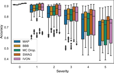
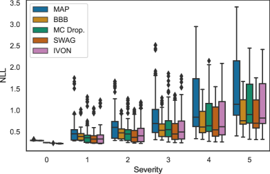
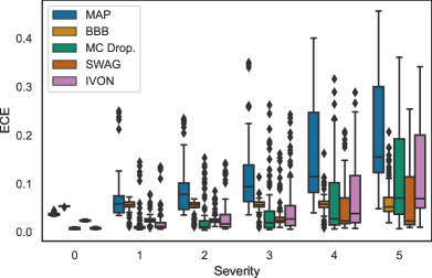
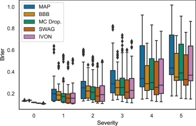
Figure 7: Distributional shift results on CIFAR-10-C with various degree of severities. Severity 0 corresponds to the in-domain case.

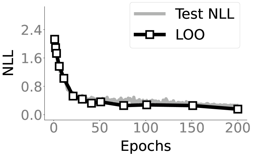
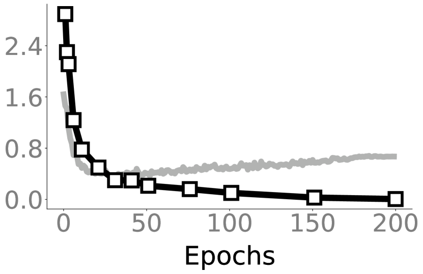
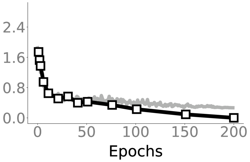
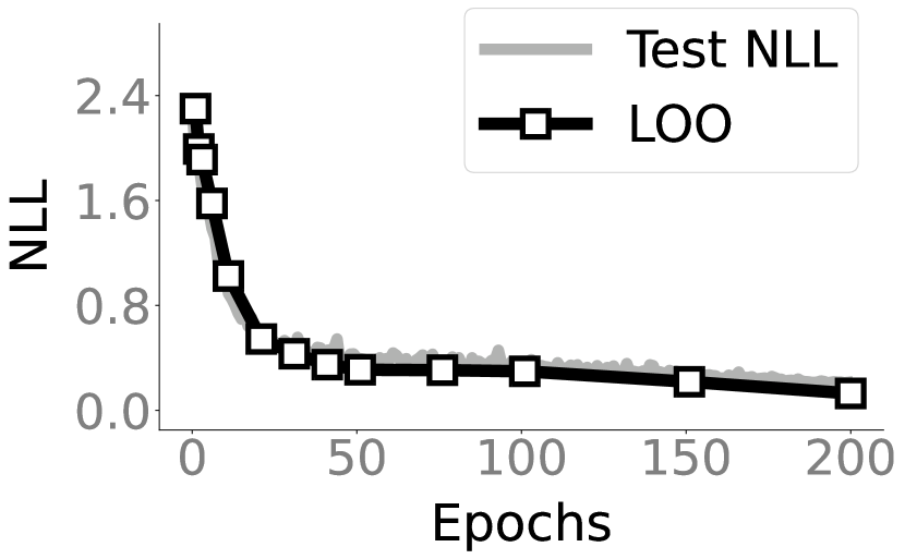
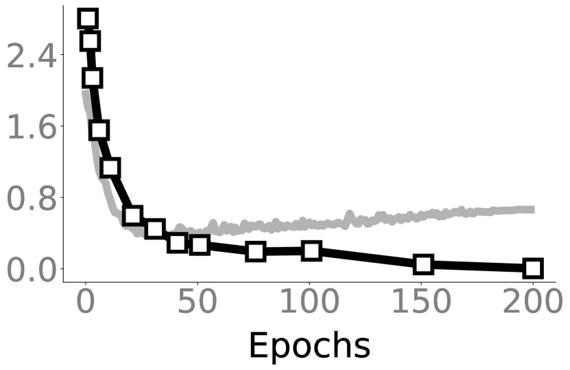
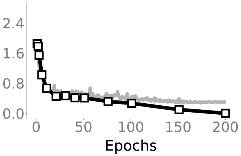
Figure 8: We predict test NLL using LOO estimation during training of two models on CIFAR10. From top to bottom the models are: ResNet–18 and PreResNet–110. IVON (first column) allows us to faithfully predict generalization, while the heuristic LOO estimates with AdamW (second column) and SGD (third column) work less well.

In general, the performance of all models decrease with increasing severity, as the classification task is getting harder. We observe that IVON keeps the best performance for low severity levels. For high severity levels, IVON is notably outperformed by SWAG. Despite this, IVON in general is still comparable to BDL baselines for high severity cases. And as an optimizer, it remains a better choice over the standard SGD training.

Method	CIFAR-10		MedMNIST		UCI
	Agree $\uparrow$	TVD $\downarrow$	Agree $\uparrow$	TVD $\downarrow$	W2 $\downarrow$
Multi-IVON	78.7%	0.198	88.4%	0.099	0.094
Multi-SWAG	77.8%	0.219	89.0%	0.098	0.166
SAE	77.3%	0.210	87.5%	0.107	0.116

Table 13: An earlier version of IVON won the NeurIPS 2021 competition on approximate inference in Bayesian deep learning (Wilson et al., 2022). The second best method used a combination of SWAG and SGLD. Third place was a Sequential Anchored Ensemble (SAE).

D.3 NeurIPS 2021 Approximate Inference Competition

An earlier version of IVON won the first place in both the light and extended track of the NeurIPS 2021 Competition on Approximate Inference in Bayesian Deep Learning (Wilson et al., 2022). The earlier version included an additional heuristic damping to $\widehat{}\mbox{$\mbox{$\mathbf{h}$}$}$ in line 3 of Alg. 1 and the weight-decay was added in line 4 rather than in lines 5 and 6. We found the damping term to be unneccesary when using a proper Hessian initialization $h_{0}$ and momentum $\beta_{2}$ and therefore removed it, making IVON easier to tune. The three highest scoring submissions to the competition are summarized in Table 13. First place is Multi-IVON (using the earlier version of IVON), which is a mixture-of-Gaussian ensemble (with uniform weights) as described in the experiments section on uncertainty estimation in the main paper. The second place solution (Multi-SWAG) uses multiple runs of SWAG to construct a mixture-of-Gaussian approximation (Izmailov et al., 2021) with SGLD (Welling & Teh, 2011) as a base optimizer. Third place was obtained by a deep ensembling method called sequential anchored ensembles (SAE) (Delaunoy & Louppe, 2021). In Table 13, Agree denotes predictive agreement with a ground-truth Bayesian posterior obtained by running Hamiltonian Monte-Carlo method on hundreds of TPUs. TVD denotes the total variation distance and W₂ the Wasserstein-2 distance between this ground-truth predictive posterior and the approximate posterior. We refer to Wilson et al. (2022) for more details.

D.4 Predicting Generalization

In Fig. 8, we conduct additional experiments with ResNet-18 and PreResNet-10 on the CIFAR10 dataset. We estimate generalization performance during training using the LOO criterion described in Sec. C.6. The accuracy of IVON is similar to the SGD baseline. IVON however results in a more faithful estimate of the generalization performance in comparison to AdamW and SGD. We evaluate the sensitivity of the models to data perturbation as described in Sec. C.6 with the difference that we compute the sensitivities as $\mbox{$\mbox{$\mathbf{e}$}$}_{i}\mbox{$\mbox{$\mathbf{v}$}$}_{i}$, where $\mbox{$\mbox{$\mathbf{v}$}$}_{i}$ are the diagonal elements of $\mbox{$\mbox{$\mathbf{V}$}$}_{i}$ and $\mbox{$\mbox{$\mathbf{v}$}$}_{i}\mbox{$\mbox{$\mathbf{e}$}$}_{i}$ is an element-wise product. For training the models, we use the same hyperparameters as in the image classification experiments. The exception is the Hessian initaliziation $h_{0}$. We do a grid search over the values $[0.01,0.05,0.1,0.5]$. We select the value that results in a faithful estimate of the generalization performance while keeping a competitive test accuracy. The Hessian initialization is set to $h_{0}=0.1$ for both models. The test accuracies are $93.68\%$ for ResNet–18 and $93.52\%$ for PreResNet–110 with predictions at the mean of the variational posterior.

References

- Blundell et al. (2015) Blundell, C., Cornebise, J., Kavukcuoglu, K., and Wierstra, D. Weight uncertainty in neural networks. In International Conference on Machine Learning (ICML), 2015.
- Cer et al. (2017) Cer, D., Diab, M., Agirre, E., Lopez-Gazpio, I., and Specia, L. SemEval-2017 task 1: Semantic textual similarity multilingual and crosslingual focused evaluation. In International Workshop on Semantic Evaluation (SemEval-2017), 2017.
- Cho et al. (2014) Cho, K., Van Merriënboer, B., Gulcehre, C., Bahdanau, D., Bougares, F., Schwenk, H., and Bengio, Y. Learning phrase representations using RNN encoder-decoder for statistical machine translation. In Conference on Empirical Methods in Natural Language Processing (EMNLP), 2014.
- Coker et al. (2022) Coker, B., Bruinsma, W. P., Burt, D. R., Pan, W., and Doshi-Velez, F. Wide mean-field Bayesian neural networks ignore the data. In International Conference on Artificial Intelligence and Statistics (AISTATS), 2022.
- Daheim et al. (2024) Daheim, N., Möllenhoff, T., Ponti, E. M., Gurevych, I., and Khan, M. E. Model merging by uncertainty-based gradient matching. In International Conference on Learning Representations (ICLR), 2024.
- Dauphin et al. (2015) Dauphin, Y., De Vries, H., and Bengio, Y. Equilibrated adaptive learning rates for non-convex optimization. Advances in Neural Information Processing Systems (NeurIPS), 2015.
- Delaunoy & Louppe (2021) Delaunoy, A. and Louppe, G. Sae: Sequential anchored ensembles. arXiv:2201.00649, 2021.
- Deng et al. (2009) Deng, J., Dong, W., Socher, R., Li, L.-J., Li, K., and Fei-Fei, L. ImageNet: A large-scale hierarchical image database. In IEEE Conference on Computer Vision and Pattern Recognition (CVPR), 2009.
- Devlin et al. (2019) Devlin, J., Chang, M.-W., Lee, K., and Toutanova, K. BERT: Pre-training of deep bidirectional transformers for language understanding. In Conference of the North American Chapter of the Association for Computational Linguistics: Human Language Technologies, Volume 1 (Long and Short Papers), 2019.
- Dolan & Brockett (2005) Dolan, W. B. and Brockett, C. Automatically constructing a corpus of sentential paraphrases. In International Workshop on Paraphrasing (IWP2005), 2005.
- Feldman & Zhang (2020) Feldman, V. and Zhang, C. What neural networks memorize and why: Discovering the long tail via influence estimation. In Advances in Neural Information Processing Systems (NeurIPS), 2020.
- Foong et al. (2020) Foong, A., Burt, D., Li, Y., and Turner, R. On the expressiveness of approximate inference in Bayesian neural networks. Advances in Neural Information Processing Systems, 33, 2020.
- Foong et al. (2019) Foong, A. Y., Li, Y., Hernández-Lobato, J. M., and Turner, R. E. ’in-between’uncertainty in bayesian neural networks. ICML Workshop on Uncertainty and Robustness in Deep Learning, 2019.
- Foret et al. (2021) Foret, P., Kleiner, A., Mobahi, H., and Neyshabur, B. Sharpness-aware minimization for efficiently improving generalization. In International Conference on Learning Representations (ICLR), 2021.
- Fortuin et al. (2022) Fortuin, V., Garriga-Alonso, A., Wenzel, F., Rätsch, G., Turner, R., van der Wilk, M., and Aitchison, L. Bayesian neural network priors revisited. In International Conference on Learning Representations (ICLR), 2022.
- Gal & Ghahramani (2016) Gal, Y. and Ghahramani, Z. Dropout as a Bayesian approximation: Representing model uncertainty in deep learning. In International Conference on Machine Learning (ICML), 2016.
- Gokaslan & Cohen (2019) Gokaslan, A. and Cohen, V. OpenWebText corpus, 2019. URL http://Skylion007.github.io/OpenWebTextCorpus.
- Graves (2011) Graves, A. Practical variational inference for neural networks. In Advances in Neural Information Processing Systems (NeurIPS), 2011.
- He et al. (2016a) He, K., Zhang, X., Ren, S., and Sun, J. Deep residual learning for image recognition. In IEEE Conference on Computer Vision and Pattern Recognition (CVPR), 2016a.
- He et al. (2016b) He, K., Zhang, X., Ren, S., and Sun, J. Identity mappings in deep residual networks. In European Conference on Computer Vision (ECCV), 2016b.
- He et al. (2023) He, P., Gao, J., and Chen, W. DeBERTav3: Improving deBERTa using ELECTRA-style pre-training with gradient-disentangled embedding sharing. In International Conference on Learning Representations (ICLR), 2023.
- Hendrycks & Dietterich (2019) Hendrycks, D. and Dietterich, T. G. Benchmarking neural network robustness to common corruptions and perturbations. In International Conference on Learning Representations (ICLR), 2019.
- Hendrycks & Gimpel (2016) Hendrycks, D. and Gimpel, K. Gaussian error linear units (GELUs). arXiv preprint arXiv:1606.08415, 2016.
- Hernández-Lobato & Adams (2015) Hernández-Lobato, J. M. and Adams, R. Probabilistic backpropagation for scalable learning of Bayesian neural networks. In International Conference on Machine Learning (ICML), 2015.
- Hoffman et al. (2013) Hoffman, M. D., Blei, D. M., Wang, C., and Paisley, J. Stochastic variational inference. J. Mach. Learn. Res. (JMLR), 14(5), 2013.
- Hoffmann et al. (2022) Hoffmann, J., Borgeaud, S., Mensch, A., Buchatskaya, E., Cai, T., Rutherford, E., de las Casas, D., Hendricks, L. A., Welbl, J., Clark, A., Hennigan, T., Noland, E., Millican, K., van den Driessche, G., Damoc, B., Guy, A., Osindero, S., Simonyan, K., Elsen, E., Vinyals, O., Rae, J. W., and Sifre, L. An empirical analysis of compute-optimal large language model training. In Advances in Neural Information Processing Systems (NeurIPS), 2022.
- Huang et al. (2017) Huang, G., Liu, Z., van der Maaten, L., and Weinberger, K. Q. Densely connected convolutional networks. In IEEE Conference on Computer Vision and Pattern Recognition (CVPR), 2017.
- Ioffe & Szegedy (2015) Ioffe, S. and Szegedy, C. Batch normalization: Accelerating deep network training by reducing internal covariate shift. In International Conference on Machine Learning, 2015.
- Izmailov et al. (2021) Izmailov, P., Vikram, S., Hoffman, M. D., and Wilson, A. G. What are Bayesian neural network posteriors really like? In International Conference on Machine Learning (ICML), 2021.
- Khan & Lin (2017) Khan, M. E. and Lin, W. Conjugate-computation variational inference: Converting variational inference in non-conjugate models to inferences in conjugate models. In International Conference on Artificial Intelligence and Statistics (AISTATS), 2017.
- Khan & Rue (2021) Khan, M. E. and Rue, H. The Bayesian learning rule. arXiv:2107.04562, 2021.
- Khan et al. (2018) Khan, M. E., Nielsen, D., Tangkaratt, V., Lin, W., Gal, Y., and Srivastava, A. Fast and scalable Bayesian deep learning by weight-perturbation in Adam. In International Conference on Machine Learning (ICML), 2018.
- Kingma & Ba (2015) Kingma, D. P. and Ba, J. Adam: A method for stochastic optimization. In International Conference on Learning Representations (ICLR), 2015. arXiv:1412.6980.
- Kingma et al. (2015) Kingma, D. P., Salimans, T., and Welling, M. Variational dropout and the local reparameterization trick. In Advances in Neural Information Processing Systems (NeurIPS), 2015.
- Koh & Liang (2017) Koh, P. W. and Liang, P. Understanding black-box predictions via influence functions. In International Conference on Machine Learning (ICML), 2017.
- Krizhevsky (2009) Krizhevsky, A. Learning multiple layers of features from tiny images. Technical report, University of Toronto, 2009.
- Lakshminarayanan et al. (2017) Lakshminarayanan, B., Pritzel, A., and Blundell, C. Simple and scalable predictive uncertainty estimation using deep ensembles. In Advances in Neural Information Processing Systems (NeurIPS), 2017.
- Le & Yang (2015) Le, Y. and Yang, X. S. Tiny imagenet visual recognition challenge. Technical report, Stanford University, 2015.
- Levesque et al. (2012) Levesque, H., Davis, E., and Morgenstern, L. The winograd schema challenge. In International Conference on the Principles of Knowledge Representation and Reasoning, 2012.
- Liang et al. (2018) Liang, S., Li, Y., and Srikant, R. Enhancing the reliability of out-of-distribution image detection in neural networks. In ICLR, 2018.
- Lin et al. (2019) Lin, W., Khan, M. E., and Schmidt, M. Fast and simple natural-gradient variational inference with mixture of exponential-family approximations. In International Conference on Machine Learning (ICML), 2019.
- Lin et al. (2020) Lin, W., Schmidt, M., and Khan, M. E. Handling the positive-definite constraint in the Bayesian learning rule. In International Conference on Machine Learning (ICML), 2020.
- Liu et al. (2023) Liu, H., Li, Z., Hall, D., Liang, P., and Ma, T. Sophia: A scalable stochastic second-order optimizer for language model pre-training. arXiv:2305.14342, 2023.
- Liu et al. (2019) Liu, Y., Ott, M., Goyal, N., Du, J., Joshi, M., Chen, D., Levy, O., Lewis, M., Zettlemoyer, L., and Stoyanov, V. RoBERTa: A robustly optimized BERT pretraining approach, 2019.
- Loshchilov & Hutter (2017) Loshchilov, I. and Hutter, F. Decoupled weight decay regularization. arXiv:1711.05101, 2017.
- Maas et al. (2011) Maas, A. L., Daly, R. E., Pham, P. T., Huang, D., Ng, A. Y., and Potts, C. Learning word vectors for sentiment analysis. In Association for Computational Linguistics (ACL), 2011.
- MacKay (1992) MacKay, D. J. C. A practical Bayesian framework for backpropagation networks. Neural Comput., 4(3):448–472, 1992.
- Maddox et al. (2019) Maddox, W. J., Izmailov, P., Garipov, T., Vetrov, D. P., and Wilson, A. G. A simple baseline for Bayesian uncertainty in deep learning. In Advances in Neural Information Processing Systems (NeurIPS), 2019.
- Möllenhoff & Khan (2023) Möllenhoff, T. and Khan, M. E. SAM as an optimal relaxation of Bayes. In International Conference on Learning Representations (ICLR), 2023.
- Netzer et al. (2011) Netzer, Y., Wang, T., Coates, A., Bissacco, A., Wu, B., and Ng, A. Y. Reading digits in natural images with unsupervised feature learning. In NIPS Workshop on Deep Learning and Unsupervised Feature Learning, 2011.
- Nickl et al. (2023) Nickl, P., Xu, L., Tailor, D., Möllenhoff, T., and Khan, M. E. The memory perturbation equation: Understanding model’s sensitivity to data. In Advances in Neural Information Processing Systems (NeurIPS), 2023.
- Nilsback & Zisserman (2008) Nilsback, M.-E. and Zisserman, A. Automated flower classification over a large number of classes. In Indian Conference on Computer Vision, Graphics and Image Processing, 2008.
- Noci et al. (2021) Noci, L., Roth, K., Bachmann, G., Nowozin, S., and Hofmann, T. Disentangling the roles of curation, data-augmentation and the prior in the cold posterior effect. In Advances in Neural Information Processing Systems (NeurIPS), 2021.
- Osawa et al. (2019) Osawa, K., Swaroop, S., Jain, A., Eschenhagen, R., Turner, R. E., Yokota, R., and Khan, M. E. Practical deep learning with Bayesian principles. Advances in Neural Information Processing Systems (NeurIPS), 2019.
- Pang & Lee (2005) Pang, B. and Lee, L. Seeing stars: Exploiting class relationships for sentiment categorization with respect to rating scales. In Association for Computational Linguistics (ACL), 2005.
- Radford et al. (2019) Radford, A., Wu, J., Child, R., Luan, D., Amodei, D., Sutskever, I., et al. Language models are unsupervised multitask learners. OpenAI blog, 1(8):9, 2019.
- Sato (2001) Sato, M.-A. Online model selection based on the variational Bayes. Neural computation, 13(7):1649–1681, 2001.
- Snoek et al. (2019) Snoek, J., Ovadia, Y., Fertig, E., Lakshminarayanan, B., Nowozin, S., Sculley, D., Dillon, J. V., Ren, J., and Nado, Z. Can you trust your model’s uncertainty? evaluating predictive uncertainty under dataset shift. In Advances in Neural Information Processing Systems (NeurIPS), 2019.
- Socher et al. (2013) Socher, R., Perelygin, A., Wu, J., Chuang, J., Manning, C. D., Ng, A., and Potts, C. Recursive deep models for semantic compositionality over a sentiment treebank. In Conference on Empirical Methods in Natural Language Processing (EMNLP), 2013.
- Srivastava et al. (2014) Srivastava, N., Hinton, G., Krizhevsky, A., Sutskever, I., and Salakhutdinov, R. Dropout: A simple way to prevent neural networks from overfitting. Journal of Machine Learning Research, 15(56):1929–1958, 2014.
- Trippe & Turner (2017) Trippe, B. and Turner, R. Overpruning in variational Bayesian neural networks. In Advances in Approximate Bayesian Inference, 2017.
- Vaswani et al. (2017) Vaswani, A., Shazeer, N., Parmar, N., Uszkoreit, J., Jones, L., Gomez, A. N., Kaiser, L., and Polosukhin, I. Attention is all you need. Advances in Neural Information Processing Systems (NeurIPS), 2017.
- Wang et al. (2018) Wang, A., Singh, A., Michael, J., Hill, F., Levy, O., and Bowman, S. GLUE: A multi-task benchmark and analysis platform for natural language understanding. In EMNLP Workshop BlackboxNLP: Analyzing and Interpreting Neural Networks for NLP, 2018.
- Warstadt et al. (2018) Warstadt, A., Singh, A., and Bowman, S. R. Neural network acceptability judgments. arXiv preprint arXiv:1805.12471, 2018.
- Welling & Teh (2011) Welling, M. and Teh, Y. W. Bayesian learning via stochastic gradient Langevin dynamics. In International Conference on Machine Learning (ICML), 2011.
- Wen et al. (2018) Wen, Y., Vicol, P., Ba, J., Tran, D., and Grosse, R. B. Flipout: Efficient pseudo-independent weight perturbations on mini-batches. In International Conference on Learning Representations (ICLR), 2018.
- Wenzel et al. (2020) Wenzel, F., Roth, K., Veeling, B. S., Swiatkowski, J., Tran, L., Mandt, S., Snoek, J., Salimans, T., Jenatton, R., and Nowozin, S. How good is the bayes posterior in deep neural networks really? In International Conference on Machine Learning (ICML), 2020.
- Williams et al. (2018) Williams, A., Nangia, N., and Bowman, S. A broad-coverage challenge corpus for sentence understanding through inference. In Conference of the North American Chapter of the Association for Computational Linguistics: Human Language Technologies, Volume 1 (Long Papers), 2018.
- Wilson et al. (2022) Wilson, A. G., Izmailov, P., Hoffman, M. D., Gal, Y., Li, Y., Pradier, M. F., Vikram, S., Foong, A., Lotfi, S., and Farquhar, S. Evaluating approximate inference in Bayesian deep learning. In Proceedings of the NeurIPS 2021 Competitions and Demonstrations Track, 2022.
- Yao et al. (2021) Yao, Z., Gholami, A., Shen, S., Mustafa, M., Keutzer, K., and Mahoney, M. W. AdaHessian: an adaptive second order optimizer for machine learning. In AAAI Conference on Artificial Intelligence (AAAI), 2021.
- Zhang et al. (2018) Zhang, G., Sun, S., Duvenaud, D., and Grosse, R. Noisy natural gradient as variational inference. In International Conference on Machine Learning (ICML), 2018.
- Zhang et al. (2015) Zhang, X., Zhao, J., and LeCun, Y. Character-level Convolutional Networks for Text Classification. In Advances in Neural Information Processing Systems (NeurIPS), 2015.