Implicit Regularization via Spectral Neural Networks
and Non-linear Matrix Sensing

Abstract

The phenomenon of implicit regularization has attracted interest in recent years as a fundamental aspect of the remarkable generalizing ability of neural networks. In a nutshell, it entails that gradient descent dynamics in many neural nets, even without any explicit regularizer in the loss function, converges to the solution of a regularized learning problem. However, known results attempting to theoretically explain this phenomenon focus overwhelmingly on the setting of linear neural nets, and the simplicity of the linear structure is particularly crucial to existing arguments. In this paper, we explore this problem in the context of more realistic neural networks with a general class of non-linear activation functions, and rigorously demonstrate the implicit regularization phenomenon for such networks in the setting of matrix sensing problems, together with rigorous rate guarantees that ensure exponentially fast convergence of gradient descent.In this vein, we contribute a network architecture called Spectral Neural Networks (abbrv. SNN) that is particularly suitable for matrix learning problems. Conceptually, this entails coordinatizing the space of matrices by their singular values and singular vectors, as opposed to by their entries, a potentially fruitful perspective for matrix learning. We demonstrate that the SNN architecture is inherently much more amenable to theoretical analysis than vanilla neural nets and confirm its effectiveness in the context of matrix sensing, via both mathematical guarantees and empirical investigations. We believe that the SNN architecture has the potential to be of wide applicability in a broad class of matrix learning scenarios.

1 Introduction

A longstanding pursuit of deep learning theory is to explain the astonishing ability of neural networks to generalize despite having far more learnable parameters than training data, even in the absence of any explicit regularization. An established understanding of this phenomenon is that the gradient descent algorithm induces a so-called implicit regularization effect. In very general terms, implicit regularization entails that gradient flow dynamics in many neural nets, even without any explicit regularizer in the loss function, converges to the solution of a regularized learning problem. In a sense, this creates a learning paradigm that automatically favors models characterized by “low complexity”.

A standard test-bed for mathematical analysis in studying implicit regularization in deep learning is the matrix sensing problem. The goal is to approximate a matrix $X^{\star}$ from a set of measurement matrices $A_{1},\dots,A_{m}$ and observations $y_{1},\dots,y_{m}$ where $y_{i}=\langle A_{i},X^{\star}\rangle$. A common approach, matrix factorization, parameterizes the solution as a product matrix, i.e., $X=UV^{\top}$, and optimizes the resulting non-convex objective to fit the data. This is equivalent to training a depth-$2$ neural network with a linear activation function.

In an attempt to explain the generalizing ability of over-parameterized neural networks, [15] first suggested the idea of an implicit regularization effect of the optimizer, which entails a bias towards solutions that generalize well. [10] investigated the possibility of an implicit norm-regularization effect of gradient descent in the context of shallow matrix factorization. In particular, they studied the standard Burer-Monteiro approach [4] to matrix factorization, which may be viewed as a depth-2 linear neural network. They were able to theoretically demonstrate an implicit norm-regularization phenomenon, where a suitably initialized gradient flow dynamics approaches a solution to the nuclear-norm minimization approach to low-rank matrix recovery [19], in a setting where the involved measurement matrices commute with each other. They also conjectured that this latter restriction on the measurement matrices is unnecessary. This conjecture was later resolved by [13] in the setting where the measurement matrices satisfy a restricted isometry property. Other aspects of implicit regularization in matrix factorization problems were investigated in several follow-up papers [14, 1, 16, 23, 17]. For instance, [1] showed that the implicit norm-regularization property of gradient flow, as studied by [10], does not hold in the context of deep matrix factorization. [16] constructed a simple $2\times 2$ example, where the gradient flow dynamics lead to an eventual blow-up of any matrix norm, while a certain relaxation of rank—the so-called e-rank—is minimized in the limit. These works suggest that implicit regularization in deep networks should be interpreted through the lens of rank minimization, not norm minimization. Incidentally, [17] have recently demonstrated similar phenomena in the context of tensor factorization.

Researchers have also studied implicit regularization in several other learning problems, including linear models [21, 24, 7], neural networks with one or two hidden layers [13, 3, 9, 12, 20]. Besides norm-regularization, several of these works demonstrate the implicit regularization effect of gradient descent in terms of other relevant quantities such as margin [21], the number of times the model changes its convexity [3], linear interpolation [12], or structural bias [9].

A natural use case scenario for investigating the implicit regularization phenomenon is the problem of matrix sensing. Classical works in matrix sensing and matrix factorization utilize convex relaxation approaches, i.e., minimizing the nuclear norm subject to agreement with the observations, and deriving tight sample complexity bound [22, 5, 19, 6, 11, 18]. Recently, many works analyze gradient descent on the matrix sensing problem. [8] and [2] show that the non-convex objectives on matrix sensing and matrix completion with low-rank parameterization do not have any spurious local minima. Consequently, the gradient descent algorithm converges to the global minimum.

Despite the large body of works studying implicit regularization, most of them consider the linear setting. It remains an open question to understand the behavior of gradient descent in the presence of non-linearities, which are more realistic representations of neural nets employed in practice.

In this paper, we make an initial foray into this problem, and investigate the implicit regularization phenomenon in more realistic neural networks with a general class of non-linear activation functions. We rigorously demonstrate the occurrence of an implicit regularization phenomenon in this setting for matrix sensing problems, reinforced with quantitative rate guarantees ensuring exponentially fast convergence of gradient descent to the best approximation in a suitable class of matrices. Our convergence upper bounds are complemented by matching lower bounds which demonstrate the optimality of the exponential rate of convergence.

In the bigger picture, we contribute a network architecture that we refer to as the Spectral Neural Network architecture (abbrv. SNN), which is particularly suitable for matrix learning scenarios. Conceptually, this entails coordinatizing the space of matrices by their singular values and singular vectors, as opposed to by their entries. We believe that this point of view can be beneficial for tackling matrix learning problems in a neural network setup. SNNs are particularly well-suited for theoretical analysis due to the spectral nature of their non-linearities, as opposed to vanilla neural nets, while at the same time provably guaranteeing effectiveness in matrix learning problems. We also introduce a much more general counterpart of the near-zero initialization that is popular in related literature, and our methods are able to handle a much more robust class of initializing setups that are constrained only via certain inequalities. Our theoretical contributions include a compact analytical representation of the gradient flow dynamics, accorded by the spectral nature of our network architecture. We demonstrate the efficacy of the SNN architecture through its application to the matrix sensing problem, bolstered via both theoretical guarantees and extensive empirical studies. We believe that the SNN architecture has the potential to be of wide applicability in a broad class of matrix learning problems. In particular, we believe that the SNN architecture would be natural for the study of rank (or e-rank) minimization effect of implicit regularization in deep matrix/tensor factorization problems, especially given the fact that e-rank is essentially a spectrally defined concept.

2 Problem Setup

Let $X^{\star}\in\mathbb{R}^{d_{1}\times d_{2}}$ be an unknown rectangular matrix that we aim to recover. Let $A_{1},\dots,A_{m}\in\mathbb{R}^{d_{1}\times d_{2}}$ be $m$ measurement matrices, and the label vector $y\in\mathbb{R}^{m}$ is generated by

$$y_{i}=\langle A_{i},X^{\star}\rangle,$$ (1)

where $\langle A,B\rangle=\mathrm{tr}(A^{\top}B)$ denotes the Frobenius inner product. We consider the following squared loss objective

$$\ell(X):=\dfrac{1}{2}\sum_{i=1}^{m}(y_{i}-\langle A_{i},X\rangle)^{2}.$$ (2)

This setting covers problems including matrix completion (where the $A_{i}$’s are indicator matrices), matrix sensing from linear measurements, and multi-task learning (in which the columns of $X$ are predictors for the tasks, and $A_{i}$ has only one non-zero column). We are interested in the regime where $m\ll d_{1}\times d_{2}$, i.e., the number of measurements is much less than the number of entries in $X^{\star}$, in which case 2 is under-determined with many global minima. Therefore, merely minimizing 2 does not guarantee correct recovery or good generalization.

Following previous works, instead of working with $X$ directly, we consider a non-linear factorization of $X$ as follows

$$X=\sum_{k=1}^{K}\alpha_{k}\Gamma(U_{k}V_{k}^{\top}),$$ (3)

where $\alpha\in\mathbb{R}$, $U_{k}\in\mathbb{R}^{d_{1}\times d},V_{k}\in\mathbb{R}^{d_{2}\times d}$, and the matrix-valued function $\Gamma:\mathbb{R}^{d_{1}\times d_{2}}\rightarrow\mathbb{R}^{d_{1}\times d_{2}}$ transforms a matrix by applying a nonlinear real-valued function $\gamma(\cdot)$ on its singular values. We focus on the over-parameterized setting $d\geq d_{2}\geq d_{1}$, i.e., the factorization does not impose any rank constraints on $X$. Let $\alpha=\{\alpha_{1},\dots,\alpha_{K}\}$ be the collection of the $\alpha_{k}$’s. Similarly, we define $U$ and $V$ to be the collections of $U_{k}$’s and $V_{k}$’s.

2.1 Gradient Flow

For each $k\in[K]$, let $\alpha_{k}(t),U_{k}(t),V_{k}(t)$ denote the trajectories of gradient flow, where $\alpha_{k}(0),U_{k}(0),V_{k}(0)$ are the initial conditions. Consequently, $X(t)=\sum_{k=1}^{K}\alpha_{k}(t)\Gamma(U_{k}(t)V_{k}(t)^{\top})$. The dynamics of gradient flow is given by the following differential equations, for $k\in[K]$

$$\partial_{t}{\alpha}_{k}=-\nabla_{\alpha_{k}}\ell(X(t)),$$

$$\partial_{t}{U}_{k}=-\nabla_{U_{k}}\ell(X(t)),$$

$$\partial_{t}{V}_{k}=-\nabla_{V_{k}}\ell(X(t)).$$ (4)

3 The SNN architecture

In this work, we contribute a novel neural network architecture, called the Spectral Neural Network (abbrv. SNN), that is particularly suitable for matrix learning problems. At the fundamental level, the SNN architecture entails an application of a non-linear activation function on a matrix-valued input in the spectral domain. This may be followed by a linear combination of several such spectrally transformed matrix-structured data.

To be precise, let us focus on an elemental neuron, which manipulates a single matrix-valued input $X$. If we have a singular value decomposition $X=\Phi\bar{X}\Psi^{\top}$, where $\Phi,\Psi$ are orthogonal matrices and $\bar{X}$ is the diagonal matrix of singular values of $X$. Let $\gamma$ be any activation function of choice. Then the elemental neuron acts on $X$ as follows :

$$X\mapsto\Phi\leavevmode\nobreak\ \gamma(\bar{X})\leavevmode\nobreak\ \Psi^{\top},$$ (5)

where $\gamma(\bar{X})$ is a diagonal matrix with the non-linearity $\gamma$ applied entrywise to the diagonal of $\bar{X}$.

Figure 1: Visualization of the anatomy of an SNN block and a depth-$D$ SNN architecture. Each SNN block takes as input $K$ matrices and outputs one matrix, both the input and output matrices are of size $\mathbb{R}^{d_{1}\times d_{2}}$. In layer $i$ of the SNN, there are $L_{i}$ blocks, which aggregate matrices from the previous layers to produce $L_{i}$ output matrices as inputs for the next layer. The number of input matrices to a block equals the number of neurons in the previous layer. For example, blocks in layer 1 have $K=L_{0}$, blocks in layer 2 have $K=L_{1}$, and blocks in layer $i$ have $K=L_{i-1}$.

A block in the SNN architecture comprises of $K\geq 1$ elemental neurons as above, taking in $K$ matrix-valued inputs $X_{1},\ldots,X_{K}$. Each input matrix $X_{i}$ is then individually operated upon by an elemental neuron, and finally, the resulting matrices are aggregated linearly to produce a matrix-valued output for the block. The coefficients of this linear combination are also parameters in the SNN architecture, and are to be learned during the process of training the network.

The comprehensive SNN architecture is finally obtained by combining such blocks into multiple layers of a deep network, as illustrated in 1.

4 Main Results

For the purposes of theoretical analysis, in the present article, we specialize the SNN architecture to focus on the setting of (quasi-) commuting measurement matrices $A_{i}$ and spectral near zero initialization; c.f. Assumptions 1 and 2 below. Similar settings have attracted considerable attention in the literature, including the foundational works of [10] and [1]. Furthermore, our analysis holds under very general analytical requirements on the activation function $\gamma$; see Assumption 3 in the following.

Assumption 1.

The measurement matrices $A_{1},\dots,A_{m}$ share the same left and right singular vectors. Specifically, there exists two orthogonal matrices $\Phi\in\mathbb{R}^{d_{1}\times d_{1}}$ and $\Psi\in\mathbb{R}^{d_{2}\times d_{2}}$, and a sequence of (rectangular) diagonal matrices $\bar{A}_{1},\dots,\bar{A}_{m}\in\mathbb{R}^{d_{1}\times d_{2}}$ such that for any $i\in[m]$, we have

$$A_{i}=\Phi\bar{A}_{i}\Psi^{\top}.$$ (6)

Let $\sigma^{(i)}$ be the vector containing the singular values of $A_{i}$, i.e., $\sigma^{(i)}=\mathrm{diag}(\bar{A}_{i})$. Furthermore, we assume that there exist real coefficients $a_{1},\dots,a_{m}$ that

$$a_{1}\sigma^{(1)}+\dots+a_{m}\sigma^{(m)}=\mathds{1}.$$ (7)

We let $\mkern 1.25mu\overline{\mkern-1.25muX\mkern-0.25mu}\mkern 0.25mu^{\star}=\Phi^{\top}X^{\star}\Psi$ and $\sigma^{\star}$ be the vector containing the diagonal elements of $\mkern 1.25mu\overline{\mkern-1.25muX\mkern-0.25mu}\mkern 0.25mu^{\star}$, i.e., $\sigma^{\star}=\mathrm{diag}(\mkern 1.25mu\overline{\mkern-1.25muX\mkern-0.25mu}\mkern 0.25mu^{\star})$. Without loss of generality, we may also assume that $\sigma^{\star}$ is coordinatewise non-zero. This can be easily ensured by adding the rectangular identity matrix (c.f. Appendix D) $cI_{d_{1}\times d_{2}}$ to $X^{*}$ for some large enough positive number $c$.

Eq. 6 postulates that the measurement matrices share the same (left- and right-) singular vectors. This holds if and only if the measurement matrices pair-wise quasi-commute in the sense that for any $i,j\in[m]$, we have

$$A_{i}A_{j}^{\top}=A_{j}A_{i}^{\top},\quad A_{i}^{\top}A_{j}=A_{j}^{\top}A_{i}.$$ (8)

A natural class of examples of such quasi-commuting measurement matrices comes from families of commuting projections. In such a scenario Eq. 7 stipulates that these projections cover all the coordinate directions, which may be related conceptually to a notion of the measurements being sufficiently informative. For example, in this setting, Eq. 7 would entail that the trace of $X^{\star}$ can be directly computed on the basis of the measurements.

Eq. 7 acts as a regularity condition on the singular values of the measurement matrices. For example, it prohibits peculiar scenarios where $\sigma^{(i)}_{1}=0$ for all $i$, i.e., all measurement matrices have $0$ as their smallest singular values, which makes it impossible to sense the smallest singular value of $X^{\star}$ from linear measurements.

Note that

$$y_{i} =\langle A_{i},X^{\star}\rangle=\mathrm{Tr}(A_{i}^{\top}X^{\star})$$ (9)

$$=\mathrm{Tr}(\Psi\bar{A}_{i}\Phi^{\top}X^{\star})=\mathrm{Tr}(\bar{A}_{i}\Phi^{\top}X^{\star}\Psi)=\langle\bar{A}_{i},\Phi^{\top}X^{\star}\Psi\rangle,$$ (10)

where in the above we use the fact that $\bar{A}_{i}=\bar{A}_{i}^{\top}$ (since $\bar{A}_{i}$ is diagonal) and the cyclic property of trace. We have

$$y_{i}=\langle\bar{A}_{i},\mkern 1.25mu\overline{\mkern-1.25muX\mkern-0.25mu}\mkern 0.25mu^{\star}\rangle=\langle\sigma^{(i)},\sigma^{\star}\rangle=\sigma^{(i)\top}\sigma^{\star},$$ (11)

where the second equality is due to $\bar{A}_{i}$ being diagonal.

We further define vectors $z^{(k)}$ and three matrices $B$, $\mathcal{C}$, and $H$ as follows

$$z_{i}^{(k)} =[\bar{U}_{k}]_{ii}[\bar{V}_{k}]_{ii}$$

$$B =\begin{bmatrix}\sigma^{(1)}\,|\,\dots\,|\,\sigma^{(m)}\end{bmatrix}\in\mathbb{R}^{d_{1}\times m}$$

$$\mathcal{C} =BB^{\top}\in\mathbb{R}^{d_{1}\times d_{1}}$$

$$H =\begin{bmatrix}\gamma(z^{(1)})\,|\,\dots\,|\,\gamma(z^{(K)})\end{bmatrix}\in\mathbb{R}^{d_{1}\times K}.$$

Under these new notations, we can write the label vector $y$ as $y=B^{\top}\sigma^{\star}$.

Assumption 2.

(Spectral Initialization) Let $\Phi$ and $\Psi$ be the matrices containing the left and right singular vectors of the measurement matrices from Assumption 1. Let $G\in\mathbb{R}^{d\times d}$ is any arbitrary orthogonal matrix. We initialize $X(0)$ such that the following condition holds: for any $k=1,\dots,K$, we have

1. $U_{k}(0)=\Phi\bar{U}_{k}(0)G$ and $V_{k}=\Psi\bar{V}(0)G$, and

2. $\bar{U}_{k}(0)$ and $\bar{V}_{k}(0)$ are diagonal, and

3. $\sum_{k=1}^{K}\alpha_{k}\gamma(\bar{U}_{k}(0)_{ii}\bar{V}_{k}(0)_{ii})\leq\sigma^{\star}_{i}$ for any $i=1,\dots,d_{1}$.

Assumption 2, especially part (c) therein, may be thought of as a much more generalized counterpart of the “near-zero” initialization which is widely used in the related literature ([10, 13, 1]). A direct consequence of Assumption 2 is that at initialization, the matrix $X(0)$ has $\Phi$ and $\Psi$ as its left and right singular vectors. As we will see later, this initialization imposes a distinctive structure on the gradient flow dynamics, allowing for an explicit analytical expression for the flow of each component of $X$.

Assumption 3.

The function $\gamma:\mathbb{R}\rightarrow\mathbb{R}$ is bounded between $[0,1]$, and is differentiable and non-decreasing on $\mathbb{R}$.

Assumption 3 imposes regularity conditions on the non-linearity $\gamma$. Common non-linearities that are used in deep learning such as Sigmoid, ReLU or tanh satisfy the differentiability and non-decreasing conditions, while the boundedness can be achieved by truncating the outputs of these functions if necessary.

Our first result provides a compact representation of the gradient flow dynamics in suitable coordinates. The derivation of this dynamics involves matrix differentials utilizing the Khatri-Rao product $\Psi\boxtimes\Phi$ of the matrices $\Psi$ and $\Phi$ (see Eq. 22 in Appendix A of the supplement).

Theorem 1.

Suppose Assumptions 1, 2, 3 hold. Then the gradient flow dynamics in 4 are

$$\partial_{t}{\boldsymbol{\alpha}} =H^{\top}\mathcal{C}(\sigma^{\star}-H\alpha),$$

$$\partial_{t}{U}_{k} =\Phi L_{k}\Psi^{\top}V_{k},\text{ and}$$

$$\partial_{t}{V}_{k} =(\Phi L_{k}\Psi^{\top})^{\top}U_{k},$$

where $L_{k}\in\mathbb{R}^{d_{1}\times d_{2}}$ is a diagonal matrix whose diagonal is given by

$$\mathrm{diag}(L_{k})=\lambda^{(k)} =[\lambda_{1}^{(k)},\dots,\lambda_{d_{1}}^{(k)}]^{\top}$$

$$=\alpha_{k}\gamma^{\prime}(z^{(k)})\circ\mathcal{C}(\sigma^{\star}-H\alpha).$$ (12)

Proof.

(Main ideas – full details in Appendix A). We leverage the fact that the non-linearity $\gamma(\cdot)$ only changes the singular values of the product matrix $U_{k}V_{k}^{\top}$ while keeping the singular vectors intact. Therefore, the gradient flow in 4 preserves the left and right singular vectors. Furthermore, by Assumption 2, $U_{k}V_{k}^{\top}$ has $\Phi$ and $\Psi$ as its left and right singular vectors at initialization, which remains the same throughout. This property also percolates to $\nabla_{U_{k}V_{k}^{\top}}\ell$. Mathematically speaking, $\nabla_{U_{k}V_{k}^{\top}}\ell$ becomes diagonalizable by $\Phi$ and $\Psi$, i.e.,

$$\nabla_{U_{k}V_{k}^{\top}}\ell=\Phi\Lambda_{k}\Psi^{\top}$$

for some diagonal matrix $\Lambda_{k}$. It turns out that $\Lambda_{k}=L_{k}$ as given in the statement of the theorem. In view of Eq. 4, this explains the expressions for $\partial_{t}{U}_{k}$ and $\partial_{t}{V}_{k}$. Finally, since $\alpha_{k}$ is a scalar, the partial derivative of $\ell$ with respect to $\alpha_{k}$ is relatively straightforward to compute. ∎

Theorem 1 provides closed-form expressions for the dynamics of the individual components of $X$, namely $\alpha_{k},U_{k}$ and $V_{k}$. We want to highlight that the compact analytical expression and the simplicity of the gradient flow dynamics on the components are a direct result of the spectral non-linearity. In other words, if we use the conventional element-wise non-linearity commonly used in deep learning, the above dynamics will be substantially more complicated, containing several Hadamard products and becoming prohibitively harder for theoretical analysis.

As a direct corollary of Theorem 1, the gradient flow dynamics on $\bar{U}_{k}$ and $\bar{V}_{k}$ are

$$\partial_{t}{\bar{U}}_{k}=L_{k}\bar{V}_{k},\quad\partial_{t}{\bar{V}}_{k}=L_{k}^{\top}\bar{U}_{k}.$$ (13)

Under Assumption 2, $\bar{U}_{k}(0)$ and $\bar{V}_{k}(0)$ are diagonal matrices. From the gradient flow dynamics in Eq. 13, and recalling that the $L_{k}$’s are diagonal, we infer that $\partial_{t}{\bar{U}}_{k}(0)$ and $\partial_{t}{\bar{V}}_{k}(0)$ are also diagonal. Consequently, $\bar{U}_{k}(t)$ and $\bar{V}_{k}(t)$ remain diagonal for all $t\geq 0$ since the gradient flow dynamics in Eq. 13 does not induce any change in the off-diagonal elements. Thus, $\bar{U}_{k}(t)\bar{V}(t)_{k}^{\top}$ also remains diagonal throughout.

A consequence of the spectral initialization is that the left and right singular vectors of $X(t)$ stay constant at $\Phi$ and $\Psi$ throughout the entire gradient flow procedure. To this end, the gradient flow dynamics is completely determined by the evolution of the singular values of $X(t)$, i.e., $H\alpha$. The next result characterizes the convergence of the singular values of $X(t)$.

Theorem 2.

Under Assumptions 1 and 2, for any $i=1,\dots,d_{1}$, there are constants $\eta_{i},C_{i}>0$ such that we have :

$$0\leq\sigma^{\star}_{i}-(H(t)\alpha(t))_{i}\leq C_{i}e^{-\eta_{i}t}.$$

On the other hand, we have the lower bound

$$\|\sigma^{\star}-(H(t)\alpha(t))\|_{2}\geq Ce^{-\eta t},$$

for some constants $\eta,C>0$.

Proof.

(Main ideas – full details in Appendix B). By part (c) of Assumption 2, at initialization, we have that $H(0)\alpha(0)\leq_{\textrm{e}}\sigma^{\star}$, in which the symbol $\leq_{\textrm{e}}$ denotes the element-wise less than or equal to relation. Therefore, to prove Theorem 2, it is sufficient to show that $H(t)\alpha(t)$ is increasing to $\sigma^{\star}$ element-wise at an exponential rate. To achieve that, we show that the evolution of $H\alpha$ over time can be expressed as

$$\partial_{t}{(H\alpha)}=4\sum_{k=1}^{K}\alpha_{k}^{2}\cdot\Big{(}\gamma^{\prime}( z^{(k)})^{2}\circ\mathcal{C}(\sigma^{\star}-H\alpha)$$

$$\circ\big{(}\int\lambda^{(k)}\circ z^{(k)}dt+C^{(k)}\big{)}\Big{)}$$

$$\quad\,\,\qquad+HH^{\top}\mathcal{C}(\sigma^{\star}-H\alpha).$$

By definition, the matrix $B$ contains the singular values of the $A_{i}$’s, and therefore its entries are non-negative. Consequently, since $\mathcal{C}=BB^{\top}$, the entries of $\mathcal{C}$ are also non-negative. By Assumption 3, we have that $\gamma(\cdot)\in[0,1]$, thus the entries of $H$ are non-negative. Finally, by Assumption 2, we have $H(0)\alpha(0)<\sigma^{\star}$ entry-wise. For these reasons, each entry in $\partial_{t}{(H\alpha)}$ is non-negative at initialization, and indeed, for each $i$, the quantity $(H\alpha)_{i}$ is increasing as long as $(H\alpha)_{i}<\sigma^{*}_{i}$ . As $H\alpha$ approaches $\sigma^{\star}$, the gradient $\partial_{t}{(H\alpha)}$ decreases. If it so happened that $H\alpha=\sigma^{\star}$ at some finite time, then $\partial_{t}{(H\alpha)}$ would exactly equal $0$, which would then cause $H\alpha$ to stay constant at $\sigma^{*}$ from then on.

Thus, each $(H\alpha)_{i}$ is non-decreasing and bounded above by $\sigma^{*}_{i}$, and therefore must converge to a limit $\leq\sigma^{*}_{i}$. If this limit was strictly smaller than $\sigma^{*}_{i}$, then by the above argument $(H\alpha)_{i}$ would be still increasing, indicating that this cannot be the case. Consequently, we may deduce that

$$\lim_{t\rightarrow\infty}H(t)\alpha(t)=\sigma^{\star}.$$

It remains to show that the convergence is exponentially fast. To achieve this, we show in the detailed proof that each entry of $\partial_{t}{H\alpha}$ is not only non-negative but also bounded away from $0$, i.e.,

$$\partial_{t}{(H\alpha)}_{i}\geq\eta_{i}(\sigma^{\star}_{i}-(H\alpha)_{i}),$$

for some constant $\eta_{i}>0$. This would imply that $H\alpha$ converges to $\sigma^{\star}$ at an exponential rate. ∎

The limiting matrix output by the network is, therefore, $\Phi\mathrm{Diag}(\sigma^{*})\Psi^{\top}$, and given the fact that $\sigma^{*}=\mathrm{diag}(\Phi^{\top}X^{*}\Psi)$, this would be the best approximation of $X^{*}$ among matrices with (the columns of) $\Phi$ and $\Psi$ as their left and right singular vectors. This is perhaps reasonable, given the fact that the sensing matrices $A_{i}$ also share the same singular vectors, and it is natural to expect an approximation that is limited by their properties. In particular, when the $A_{i}$ are symmetric and hence commuting, under mild linear independence assumptions, $\Phi\mathrm{Diag}(\sigma^{*})\Psi^{\top}$ would be the best approximation of $X^{*}$ in the algebra generated by the $A_{i}$-s, which is again a natural class given the nature of the measurements.

We are now ready to rigorously demonstrate the phenomenon of implicit regularization in our setting. To this end, following the gradient flow dynamics, we are interested in the behavior of $X_{\infty}$ in the limit when time goes to infinity.

Theorem 3.

Let $X_{\infty}=\lim_{t\rightarrow\infty}X(t)$. Under Assumptions 1 and 2, the following hold:

1. $\ell(X_{\infty})=0$, and

2. $X_{\infty}$ solves the optimization problem

   $$\min_{X\in\mathbb{R}^{d_{1}\times d_{2}}}\lVert X\rVert_{*}\quad\textrm{subject to}\quad y_{i}=\langle A_{i},X\rangle\,\,\forall i\in[m].$$ (14)

Proof.

(Main ideas – full details in Appendix C). A direct corollary of Theorem 2 is that

$$H(\infty)\alpha(\infty)=\sigma^{\star}.$$

By some algebraic manipulations, we can show that the limit of $X$ takes the form

$$X_{\infty}=\Phi\Big{[}\mathrm{Diag}(\sigma^{\star})\Big{]}\Psi^{\top}.$$

Now, let us look at the prediction given by $X_{\infty}$. For any $i=1,\dots,m$, we have

$$\langle A_{i},X_{\infty}\rangle =\langle\Phi\bar{A}_{i}\Psi^{\top},\Phi\mathrm{Diag}(\sigma^{\star})\Psi^{\top}\rangle=\langle\sigma^{(i)},\sigma^{\star}\rangle=y_{i},$$

where the last equality holds due to 11. This implies that $\ell(X_{\infty})=0$, proving (a).

To prove (b), we will show that $X_{\infty}$ satisfies the Karush-Kuhn-Tucker (KKT) conditions of the optimization problem stated in Eq. 14. The conditions are

$$\exists\nu\in\mathbb{R}^{m}\textrm{ s.t. }\quad\forall i\in[m],\langle A_{i},X\rangle=y_{i}\quad\textrm{and}$$

$$\nabla_{X}\lVert X\rVert_{*}+\sum_{i=1}^{m}\nu_{i}A_{i}=0.$$

The solution matrix $X_{\infty}$ satisfies the first condition as proved in part (a). As for the second condition, note first that the gradient of the nuclear norm of $X_{\infty}$ is given by

$$\nabla\lVert X_{\infty}\rVert=\Phi\Psi^{\top}.$$

Therefore the second condition becomes

$$\Phi\Psi^{\top}+\sum_{i=1}^{m}\nu_{i}A_{i}=0$$

$$\Leftrightarrow\quad\Phi\Big{(}I-\sum_{i=1}^{m}\nu_{i}\bar{A}_{i}\Big{)}\Psi^{\top}=0\quad\Leftrightarrow\quad B\nu=\mathds{1}.$$

However, by Assumption 1, the vector $\mathds{1}$ lies in the column space of $B$, which implies the existence of such a vector $\nu$. This concludes the proof of part (b). ∎

5 Numerical studies

In this section, we present numerical studies to complement our theoretical analysis.

We highlight that gradient flow can be viewed as gradient descent with an infinitesimal learning rate. Therefore, the gradient flow model serves as a reliable proxy for studying gradient descent when the learning rate is sufficiently small. Throughout our experiments, we shall consider gradient descent with varying learning rates, and demonstrate that the behavior suggested by our theory is best achieved using small learning rates.

The synthetic data used in our experiment is generated by $X^{\star}=\tilde{X}\tilde{X}^{T}\in\mathbb{R}^{10\times 10}$ where each entry of $\tilde{X}\in\mathbb{R}^{10\times 6}$ is randomly sampled from uniformly on $[0,1]$ and normalize so that $\|X^{\star}\|=1$.

5.1 Numerical verification of theoretical results

In the first experiment, we follow Assumption 1 and Assumption 2 to generate measurement matrices and initialize our network. For every $k=1,K=2$, we initialize $\bar{U}(0)$ and $\bar{V}(0)$ to be diagonal matrices, whose diagonal entries are sampled uniformly from $[0,1]$, sorted in descending order, and set $U(0)=\Phi\bar{U}(0)G,V(0)=\Psi^{\top}\bar{V}(0)G$ where $G$ is a random orthogonal matrix. The rest of the parameters are sampled uniformly from $[0,1]$, and we use the hyperbolic tangent $\gamma(x)=(e^{x}-e^{-x})/(e^{x}+e^{-x})$ as activation.

For every measurement matrix $A_{i}$ where $i=1,\dots,m$, with $m=50$, we sample each entry of the diagonal matrix $\bar{A}_{i}$ from the uniform distribution on $[0,1]$, sort them in decreasing order, and set $A_{i}=\Phi\bar{A}_{i}\Psi^{\top}$. The measurements are recorded as $y_{i}=\langle A_{i},X^{\star}\rangle+10^{-2}\epsilon_{i}$, where $\epsilon_{i}$ is sampled from the standard Gaussian distribution, $i=1,\ldots,m$.

We illustrate the numerical results in Figure 2. One can observe that singular values of the solution matrices converge to $\sigma^{\star}$ at an exponential rate as suggested by Theorem 2, while the nuclear norm values also converge to $\|X^{\star}\|=1$. We re-emphasize that our theoretical results are for gradient flow, which only acts as a good surrogate to study gradient descent when the learning rates are infinitesimally small. As a result, our theory cannot characterize the behavior of gradient descent algorithm with substantially large learning rates. We show the evolution of the nuclear norm over time. Interestingly, but perhaps not surprisingly, the choice of the learning rate dictates the speed of convergence. Moderate values of the learning rate seem to yield the quickest convergence to stationarity.

Figure 2: The evolution of training error (left panel), nuclear norm (middle panel), and 3 leading singular values (right panel) over time with learning rates (lr) of different magnitudes.

5.2 Experiments violating Assumptions 1 and 2

In the second experiment where Assumptions 1 and 2 do not hold, we show that our model is still able to recover the original images with reasonable quality, which indicates its effectiveness in solving matrix sensing problems. Each entry in the measurement matrix $A_{i}\in\mathbb{R}^{n\times n}$ ($i=1,\dots,m=50)$ now is generated by sampling independently from the standard Gaussian distribution, and $U(0),V(0)$ are initialized as diagonal matrices, whose diagonal entries are $10^{-4}+10^{-6}\epsilon$ where $\epsilon$ is sampled from the standard Gaussian distribution. We report and compare the numerical results with the naive linear regression model $X=\arg\min_{X}\frac{1}{2}\sum_{i=1}^{m}\left(y_{i}-\langle A_{i},X\rangle\right)^{2}$ and depth-3 factorization model
$X=\arg\min_{W_{1},W_{2},W_{3}}\frac{1}{2}\sum_{i=1}^{m}\left(y_{i}-\langle A_{i},W_{1}W_{2}W_{3}\rangle\right)^{2}$ in Figure 3 and Figure 4. In particular, the linear regression and depth-3 factorization models are initialized at $X(0)=0,W_{1}(0)=W_{2}(0)=W_{3}(0)=10^{-4}I$.

We observe that the linear regression model yields solution matrices with low training errors but their nuclear norm values ($\approx 1.5$) and leading singular values are notably different from the ground-truth. This overfitting phenomenon could be partially explained by the setting that the number of observations $m=50$ is smaller than the number of variables $n^{2}=100$. In contrast, our network snn produces lower nuclear norm values ($\approx 0.95$) and leading singular values are closer to the ground-truth. This numerically verifies our Theorem 3, affirming that our network has a preference for solutions with a lower nuclear norm among all feasible solutions satisfying $m$ observations constraints. Corresponding to lower nuclear norm values, one also notes that our constructed matrices have better reconstruction quality ($\texttt{psnr}\approx 20$) than the linear regression model ($\texttt{psnr}\approx 7$). This highlights that the regularization phenomenon potentially yields favorable recovery solutions in practice. In addition, we find that the depth-3 factorization model returns solutions with lower effective ranks. However, these outcomes might not be favorable in solving matrix sensing problems as one can see the reconstruction errors are more significant than our model.

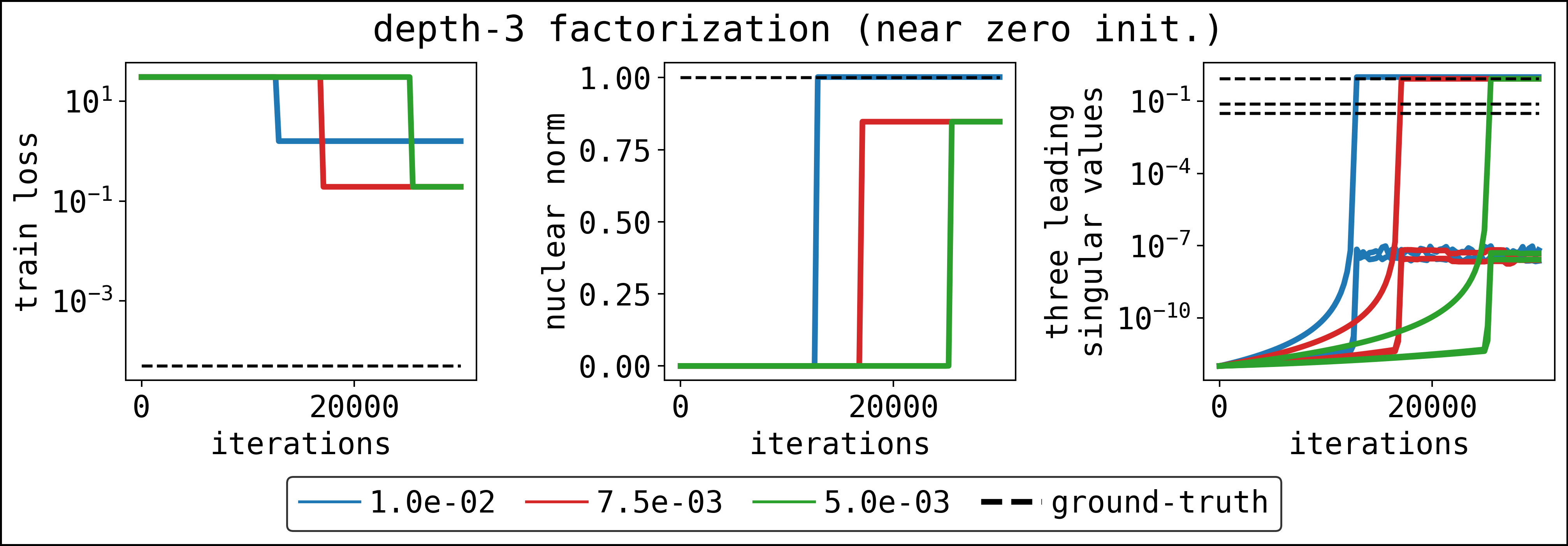
Figure 3: The evolution of training error (left panel), nuclear norm (middle panel), 3 leading singular values (right panel) over time with different learning rates (lr) of different models.

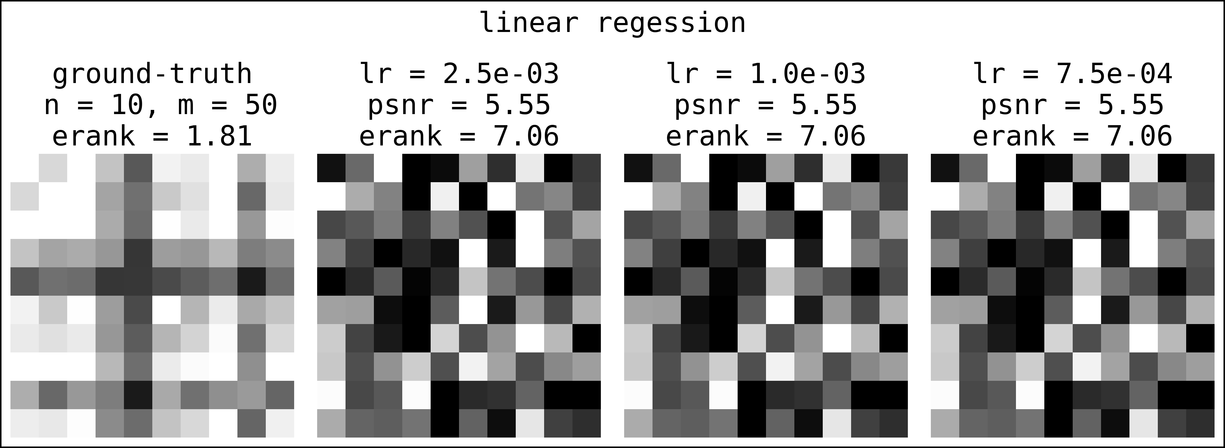
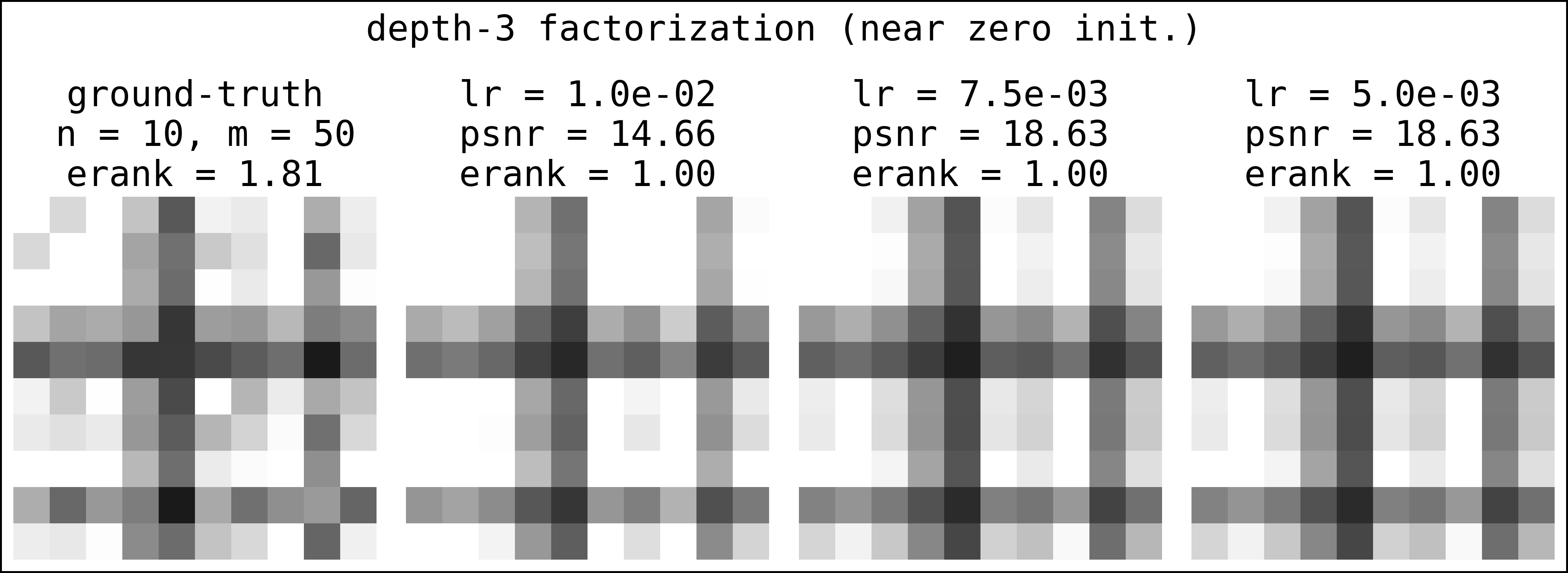
Figure 4: The reconstruction images over time with different learning rates (lr) of different models.

5.3 Real image reconstruction task

In the third experiment, we illustrate the numerical results where the ground-truth $X^{\star}$ are real images retrieved from the MNIST dataset. The measurement matrices and initializations are generated as in Section 5.2, and $K=4$. The numerical performances reported in Figure 5 suggest that the spectral regularization phenomena could be regarded as a denoising methodology in certain circumstances where the number of observations is low.

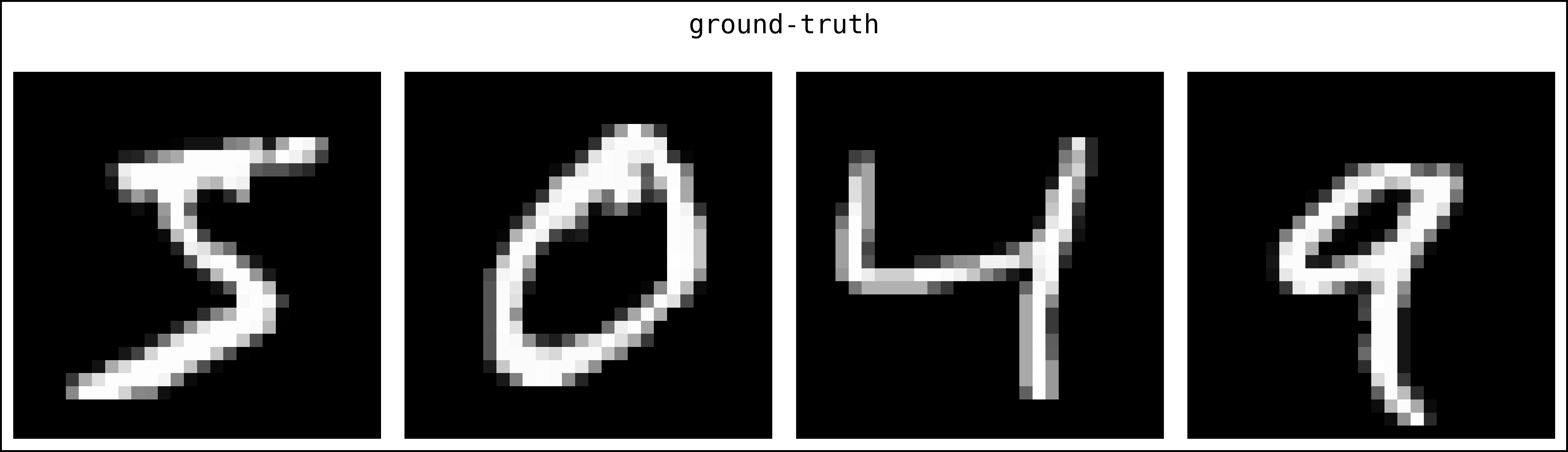
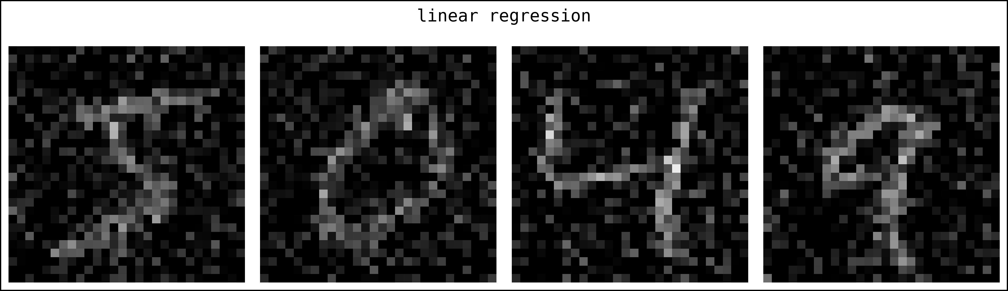
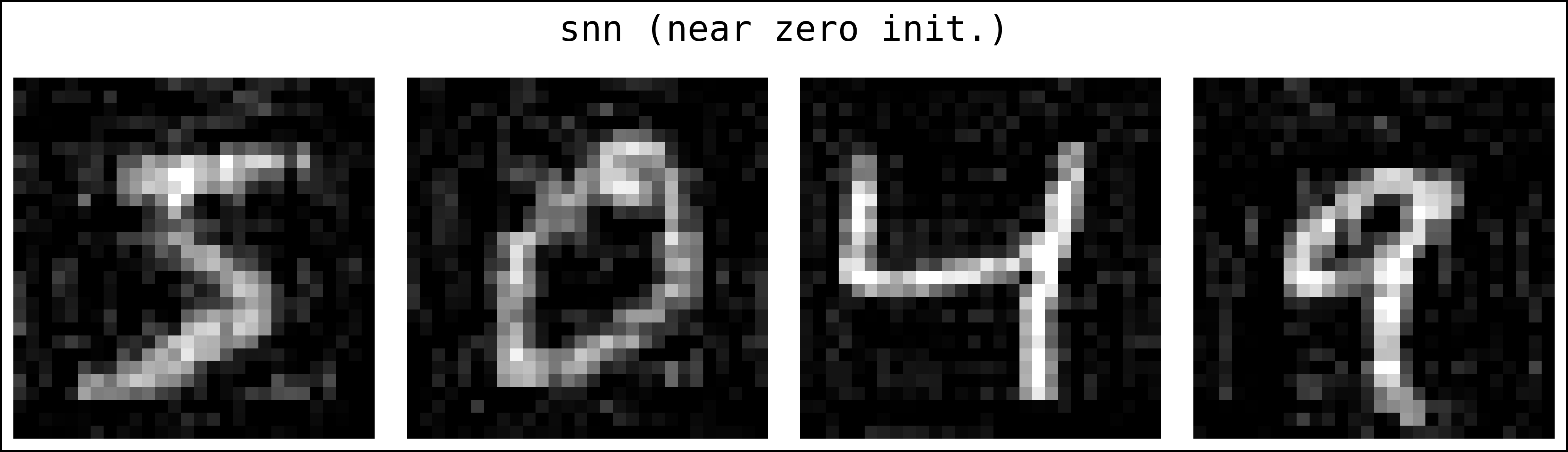
Figure 5: Top row: ground-truth $X^{\star}$, middle row & bottom row: recovering images by linear regression and our model.

6 Summary of contributions and future directions

In this work, we investigate the phenomenon of implicit regularization via gradient flow in neural networks, using the problem of matrix sensing as a canonical test bed. We undertake our investigations in the more realistic scenario of non-linear activation functions, compared to the mostly linear structure that has been explored in the literature. In this endeavor, we contribute a novel neural network architecture called Spectral Neural Network (SNN) that is particularly well-suited for matrix learning problems. SNNs are characterized by a spectral application of a non-linear activation function to matrix-valued input, rather than an entrywise one. Conceptually, this entails coordinatizing the space of matrices by their singular values and singular vectors, as opposed to by their entries. We believe that this perspective has the potential to gain increasing salience in a wide array of matrix learning scenarios. SNNs are particularly well-suited for theoretical analysis due to their spectral nature of the non-linearities, as opposed to vanilla neural nets, while at the same time provably guaranteeing effectiveness in matrix learning problems. We also introduce a much more general counterpart of the near-zero initialization that is popular in related literature, and our methods are able to handle a much more robust class of initializing setups that are constrained only via certain inequalities. Our theoretical contributions include a compact analytical representation of the gradient flow dynamics, accorded by the spectral nature of our network architecture. We demonstrate a rigorous proof of exponentially fast convergence of gradient descent to an approximation to the original matrix that is best in a certain class, complemented by a matching lower bound, Finally, we demonstrate the matrix-valued limit of the gradient flow dynamics achieves zero training loss and is a minimizer of the matrix nuclear norm, thereby rigorously establishing the phenomenon of implicit regularization in this setting.

Our work raises several exciting possibilities for follow-up and future research. A natural direction is to extend our analysis to extend our detailed analysis to the most general setting when the sensing matrices $A_{i}$ are non-commuting. An investigation of the dynamics in the setting of discrete time gradient descent (as opposed to continuous time gradient flow) is an important question, wherein the optimal choice of the learning rate appears to be an intriguing question, especially in the context of our numerical studies (c.f. Fig. 3). Finally, it would be of great interest to develop a general theory of SNNs for applications of neural network-based techniques to matrix learning problems.

Appendix A Proof of Theorem 1

Before presenting the Proof of Theorem 1, we define the few notations. Let $A\in\mathbb{R}^{d_{1}\times d_{2}},d_{1}<d_{2}$ be a rectangular matrix and $a\in\mathbb{R}^{d_{1}}$ be a vector. We let $A_{ij}$ denote the $(i,j)$-entry of $A$, $A_{i\ast}$ denote the $i$-th row of $A$, and $A_{\ast j}$ denote the $j$-th column of $A$. We define the following functions on the matrix $A$.

$$\mathrm{vec}:\mathbb{R}^{d_{1}\times d_{2}}\rightarrow\mathbb{R}^{d_{1}d_{2}}\quad \mathrm{vec}(A)=\begin{bmatrix}A_{\ast 1}^{\top}&\dots&A_{\ast d_{2}}^{\top}\end{bmatrix}^{\top}$$ (15)

$$\mathrm{diag}:\mathbb{R}^{d_{1}\times d_{2}}\rightarrow\mathbb{R}^{d_{1}} \mathrm{diag}(A)=[A_{11}\dots A_{d_{1}d_{1}}]^{\top}$$ (16)

$$\mathrm{Diag}:\mathbb{R}^{d_{1}}\rightarrow\mathbb{R}^{d_{1}\times d_{2}} \mathrm{Diag}(a)=\begin{bmatrix}a_{1}&\cdots&0&0&\cdots&0\\ \vdots&\ddots&\vdots&\vdots&\ddots&\vdots\\ 0&\cdots&a_{d_{1}}&0&\cdots&0\\ \end{bmatrix}.$$ (17)

We are now ready to present the Proof of Theorem 1. We first recall the definition of $X$ in Eq. 3

$$X=\sum_{k=1}^{K}\alpha_{k}\Gamma(U_{k}V_{k}^{\top}),$$

where $\Gamma(\cdot)$ is a matrix-valued function that applies a non-linear scalar-valued function $\gamma(\cdot)$ on the matrix’s singular values. Under Assumption 1, we can write $U_{k}$ and $V_{k}$ as

$$U_{k}V_{k}^{\top} =(\Phi\bar{U}_{k}\Psi^{T}G)(G^{\top}\bar{V}_{k}^{\top}\Psi^{\top})=\Phi\bar{U}_{k}\bar{V}_{k}^{\top}\Psi^{\top}.$$

Since both $\bar{U}_{k}$ and $\bar{V}_{k}$ are diagonal matrices, their product $\bar{U}_{k}\bar{V}_{k}^{\top}$ is also diagonal. Consequently, we can write

$$\Gamma(U_{k}V_{k}^{\top}) =\Phi\gamma(\bar{U}_{k}\bar{V}_{k}^{\top})\Psi^{\top},$$

where $\gamma(\cdot)$ is applied entry-wise on the matrix $\bar{U}_{k}\bar{V}_{k}^{\top}$. We can now write the matrix $X$ as

$$X=\sum_{k=1}^{K}\alpha_{k}\Phi\gamma(\bar{U}_{k}\bar{V}_{k}^{\top})\Psi^{\top}=\Phi\bigg{(}\sum_{k=1}^{K}\alpha_{k}\gamma(\bar{U}_{k}\bar{V}_{k}^{\top})\bigg{)}\Psi^{\top}.$$ (18)

For notational convenience, we define the following notations to be used throughout this section:

$$\mkern 1.25mu\overline{\mkern-1.25muX\mkern-0.25mu}\mkern 0.25mu =\sum_{k=1}^{K}\alpha_{k}\gamma(\bar{U}_{k}\bar{V}_{k}^{\top})\in\mathbb{R}^{d_{1}\times d_{2}}:\textrm{Diagonal matrix containing the singular values of $X$}$$ (19)

$$\mkern 1.25mu\overline{\mkern-1.25mu\mathbf{x}\mkern-0.25mu}\mkern 0.25mu =\mathrm{diag}(\mkern 1.25mu\overline{\mkern-1.25muX\mkern-0.25mu}\mkern 0.25mu)\in\mathbb{R}^{d_{1}}:\textrm{Vector containing the singular values of $X$}$$ (20)

$$\mathbf{x} =\mathrm{vec}(X)\in\mathbb{R}^{d_{1}d_{2}}:\textrm{The matrix $X$ expressed as a vector}$$ (21)

$$\Theta =\Psi\boxtimes\Phi\in\mathbb{R}^{d_{1}d_{2}\times d_{1}}:\textrm{Khatri--Rao product between $\Psi$ and $\Phi$}$$ (22)

$$G =\dfrac{\partial\ell(X)}{\partial X}=-\sum_{j=1}^{m}(y_{j}-\langle A_{j},X\rangle)A_{j}\in\mathbb{R}^{d_{1}\times d_{2}}:\textrm{Gradient of $\ell(X)$ with respect to $X$}$$ (23)

$$\mathbf{g} =\mathrm{vec}(G)\in\mathbb{R}^{d_{1}d_{2}}:\textrm{The gradient $G$ expressed as a vector}$$ (24)

$$Z_{k} =U_{k}V_{k}^{\top}\in\mathbb{R}^{d_{1}\times d_{2}}:\textrm{Product matrix between $U_{k}$ and $V_{k}^{\top}$}.$$ (25)

The Khatri–Rao product in Eq. 22 is defined as follows: the columns of the matrix $\Theta$ are Kronecker products of the corresponding columns of $\Psi$ and $\Phi$. In other words, the $i$-th column of $\Theta$ can be expressed as the vectorization of the outer product between the $i$-th column of $\Phi$ and the $i$-th column of $\Psi$, i.e.,

$$\Theta_{\ast i}=\mathrm{vec}(\phi_{i}\psi_{i}^{\top}).$$ (26)

We shall see in the next paragraph that by leveraging the Khatri–Rao product, we can write the differentials of many quantities of interest compactly, facilitating the derivation of the gradient flow dynamics in Theorem 4.

Therefore, we can use the Khatri–Rao product to expand $\mathrm{vec}(X)$ as follows:

$$X =\Phi\mkern 1.25mu\overline{\mkern-1.25muX\mkern-0.25mu}\mkern 0.25mu\Psi^{\top}=\sum_{i=1}^{d_{1}}\mkern 1.25mu\overline{\mkern-1.25muX\mkern-0.25mu}\mkern 0.25mu_{ii}\phi_{i}\psi_{i}^{\top}$$ (27)

$$\mathbf{x} =\mathrm{vec}(X)=\sum_{i=1}^{d_{1}}\mkern 1.25mu\overline{\mkern-1.25muX\mkern-0.25mu}\mkern 0.25mu_{ii}\mathrm{vec}(\phi_{i}\psi_{i}^{\top})=\sum_{i=1}^{d_{1}}\mkern 1.25mu\overline{\mkern-1.25muX\mkern-0.25mu}\mkern 0.25mu_{ii}\Theta_{\ast i}=\Theta\mkern 1.25mu\overline{\mkern-1.25mu\mathbf{x}\mkern-0.25mu}\mkern 0.25mu.$$ (28)

From here, we can write the differential of $X$ as

$$d\mathbf{x}=\Theta d\mkern 1.25mu\overline{\mkern-1.25mu\mathbf{x}\mkern-0.25mu}\mkern 0.25mu.$$ (29)

Since $\mkern 1.25mu\overline{\mkern-1.25mu\mathbf{x}\mkern-0.25mu}\mkern 0.25mu_{i}$ is the $i$-th singular value of the matrix $X$, we can express the differential of $\mkern 1.25mu\overline{\mkern-1.25mu\mathbf{x}\mkern-0.25mu}\mkern 0.25mu_{i}$ as follows:

$$d\mkern 1.25mu\overline{\mkern-1.25mu\mathbf{x}\mkern-0.25mu}\mkern 0.25mu_{i}=\langle\phi_{i}\psi_{i}^{\top},dX\rangle=\langle\phi_{i}\psi_{i}^{\top},\alpha_{k}\gamma^{\prime}(z_{i}^{(k)})dZ_{k}\rangle=\langle\alpha_{k}\gamma^{\prime}(z_{i}^{(k)})\phi_{i}\psi_{i}^{\top},dZ_{k}\rangle,$$ (30)

where the first equality is due to Eq. 3, and the second equality is due to $\alpha_{k}$ and $\gamma^{\prime}(z_{i}^{(k)})$ being scalars. Notice that we can write the vector $\mkern 1.25mu\overline{\mkern-1.25mu\mathbf{x}\mkern-0.25mu}\mkern 0.25mu$ as a sum over its entries as follow

$$\mkern 1.25mu\overline{\mkern-1.25mu\mathbf{x}\mkern-0.25mu}\mkern 0.25mu =\sum_{i=1}^{d_{1}}\mkern 1.25mu\overline{\mkern-1.25mu\mathbf{x}\mkern-0.25mu}\mkern 0.25mu_{i}\cdot\mathbf{e}_{i},$$

where $\mathbf{e}_{i}$ denote the $i$-th canonical basis vectors of $\mathbb{R}^{d_{1}}$. We have

$$d\mkern 1.25mu\overline{\mkern-1.25mu\mathbf{x}\mkern-0.25mu}\mkern 0.25mu =\sum_{i=1}^{d_{1}}d\mkern 1.25mu\overline{\mkern-1.25mu\mathbf{x}\mkern-0.25mu}\mkern 0.25mu_{i}\cdot\mathbf{e}_{i}=\sum_{i=1}^{d_{1}}\langle\alpha_{k}\gamma^{\prime}(z_{i}^{(k)})\phi_{i}\psi_{i}^{\top},dZ_{k}\rangle\cdot\mathbf{e}_{i}=\alpha_{k}\gamma^{\prime}(z_{i}^{(k)})\Big{\langle}\sum_{i=1}^{d_{1}}\mathbf{e}_{i}\star\phi_{i}\psi_{i}^{\top},dZ_{k}\Big{\rangle},$$ (31)

where $\star$ denotes the tensor product, i.e., $\mathbf{e}_{i}\star\phi_{i}\psi_{i}^{\top}\in\mathbb{R}^{d_{1}\times d_{1}\times d_{2}}$ is a third-order tensor. Since $dZ_{k}$ has dimension $d_{1}\times d_{2}$, the above Frobenius product returns a vector of dimension $d_{1}$, which matches that of $d\mkern 1.25mu\overline{\mkern-1.25mu\mathbf{x}\mkern-0.25mu}\mkern 0.25mu$. Substituting Eq. 31 this into the differential of $\ell(X)$ gives

$$d\ell(X) =\Big{\langle}\dfrac{\partial\ell}{\partial X},dX\Big{\rangle}=\langle G,dX\rangle=\mathbf{g}^{\top}d\mathbf{x}=\mathbf{g}^{\top}\Theta d\mkern 1.25mu\overline{\mkern-1.25mu\mathbf{x}\mkern-0.25mu}\mkern 0.25mu$$

$$=\alpha_{k}\gamma^{\prime}(z_{i}^{(k)})\Big{\langle}\sum_{i=1}^{d_{1}}(\mathbf{g}^{\top}\Theta\mathbf{e}_{i})(\phi_{i}\psi_{i}^{\top}),dZ_{k}\Big{\rangle}.$$ (32)

Let us define the scalar $\lambda_{i}^{(k)}$ as

$$\lambda_{i}^{(k)} =-\alpha_{k}\gamma^{\prime}(z_{i}^{(k)})\>\mathbf{g}^{\top}\Theta\mathbf{e}_{i}$$

$$\stackrel{{\scriptstyle(a)}}{{=}}-\alpha_{k}\gamma^{\prime}(z_{i}^{(k)})\>\mathbf{g}^{\top}\Theta_{\ast i}$$

$$\stackrel{{\scriptstyle(b)}}{{=}}-\alpha_{k}\gamma^{\prime}(z_{i}^{(k)})\>\mathbf{g}^{\top}\mathrm{vec}(\phi_{i}\psi_{i}^{\top})$$

$$=-\alpha_{k}\gamma^{\prime}(z_{i}^{(k)})\langle G,\phi_{i}\psi_{i}^{\top}\rangle$$

$$\stackrel{{\scriptstyle(c)}}{{=}}\alpha_{k}\gamma^{\prime}(z_{i}^{(k)})\Big{\langle}\sum_{j=1}^{m}(y_{j}-\langle A_{j},X\rangle)A_{j},\phi_{i}\psi_{i}^{\top}\Big{\rangle}$$

$$=\alpha_{k}\gamma^{\prime}(z_{i}^{(k)})\sum_{j=1}^{m}(y_{j}-\langle A_{j},X\rangle)\Big{\langle}A_{j},\phi_{i}\psi_{i}^{\top}\Big{\rangle}$$

$$\stackrel{{\scriptstyle(d)}}{{=}}\alpha_{k}\gamma^{\prime}(z_{i}^{(k)})\sum_{j=1}^{m}\Big{(}\langle\sigma^{(j)},\sigma^{\star}\rangle-\sum_{l=1}^{K}\alpha_{l}\langle\sigma^{(j)},\gamma(z^{(l)})\rangle\Big{)}\cdot\sigma_{i}^{(j)}$$

$$\stackrel{{\scriptstyle(e)}}{{=}}\alpha_{k}\gamma^{\prime}(z_{i}^{(k)})\sum_{j=1}^{m}\Big{(}B^{\top}\sigma^{\star}-B^{\top}H\alpha\Big{)}\cdot\sigma_{i}^{(j)}$$

$$=\alpha_{k}\gamma^{\prime}(z_{i}^{(k)})\cdot\mathrm{row}_{i}(B)B^{\top}(\sigma^{\star}-H\alpha),$$

where $(a)$ is due to $\Theta\mathbf{e}_{i}$ equals to the $i$-column of $\Theta$, $(b)$ is due to Eq. 26, $(c)$ is due to the definition of the matrix $G$ in Eq. 23, $(d)$ is due to Eq. 11, and $(e)$ is due to the definitions of $B$ and $H$.

Let $\lambda^{(k)}\in\mathbb{R}^{d_{1}}$ denote the vector containing the $\lambda_{i}^{(k)}$, we can write

$$\lambda^{(k)}=\alpha_{k}\cdot\gamma^{\prime}(z^{(k)})\circ BB^{\top}(\sigma^{\star}-H\alpha)=\alpha_{k}\cdot\gamma^{\prime}(z^{(k)})\circ\mathcal{C}(\sigma^{\star}-H\alpha).$$ (33)

The differential of $d\ell(X)$ becomes

$$d\ell(X) =-\Big{\langle}\sum_{i=1}^{d_{1}}\lambda_{i}^{(k)}\phi_{i}\psi_{i}^{\top},dZ_{k}\Big{\rangle},$$

$$\dfrac{\partial\ell(X)}{\partial Z_{k}} =-\sum_{i=1}^{d_{1}}\lambda_{i}^{(k)}\phi_{i}\psi_{i}^{\top}=-\Phi L^{(k)}\Psi^{\top},$$ (34)

where $L^{(k)}$ is a diagonal matrix whose diagonal entries are $\lambda_{i}^{(k)}$, i.e., $L^{(k)}=\mathrm{Diag}(\lambda^{(k)})$. Since $Z_{k}=U_{k}V_{k}^{\top}$, we have

$$\dfrac{\partial\ell(X)}{\partial U_{k}} =-\sum_{i=1}^{d_{1}}\lambda_{i}^{(k)}\phi_{i}\psi_{i}^{\top}=-\Phi L^{(k)}\Psi^{\top}V_{k},$$ (35)

$$\dfrac{\partial\ell(X)}{\partial V_{k}} =-\sum_{i=1}^{d_{1}}\lambda_{i}^{(k)}\phi_{i}\psi_{i}^{\top}=-(\Phi L^{(k)}\Psi^{\top})^{\top}U_{k}.$$ (36)

This concludes the proof for the gradient flow dynamics on $U_{k}$ and $V_{k}$. In the remaining, we shall derive the gradient of $\ell(X)$ with respect to the scalar $\alpha_{k}$.

$$\dfrac{\partial\ell(X)}{\partial\alpha_{k}} =-\sum_{j=1}^{m}(y_{j}-\langle A_{j},X\rangle)\langle\Gamma(U_{k}V_{k}^{\top}),A_{j}\rangle$$

$$=-\sum_{j=1}^{m}\Big{(}\big{\langle}\sigma^{(i)},\sigma^{\star}-\sum_{l=1}^{K}\alpha_{l}\gamma(z^{(l)})\big{\rangle}\cdot\big{\langle}\sigma^{(i)},\gamma(z^{(k)})\big{\rangle}\Big{)}$$

$$=-\gamma(z^{(k)})^{\top}\mathcal{C}\Big{(}\sigma^{\star}-\sum_{l=1}^{K}\alpha_{l}\gamma(z^{(l)})\Big{)}$$

$$=-\gamma(z^{(k)})^{\top}\mathcal{C}(\sigma^{\star}-H\alpha),$$

where the second equality is due to Eq. 11. Consequently, the gradient of $\ell(X)$ with respect to the vector $\alpha$ is

$$\dfrac{\partial\ell(X)}{\partial\alpha}=-H^{\top}\mathcal{C}(\sigma^{\star}-H\alpha),$$ (37)

which concludes the proof of Theorem 1.

Appendix B Proof of Theorem 2

Let us direct our attention to the evolution of the diagonal elements. Restricting 13 to the diagonal elements gives us a system of differential equations for each $i\in[m]$:

$$[\partial_{t}{\bar{U}}_{k}]_{ii}=\lambda_{i}^{(k)}[\bar{V}_{k}]_{ii},\quad[\partial_{t}{\bar{V}}_{k}]_{ii}=\lambda_{i}^{(k)}[\bar{U}_{k}]_{ii}.$$ (38)

We can re-write the above into a single matrix differential equation as

$$\partial_{t}{\begin{bmatrix}[\bar{U}_{k}]_{ii}\\ [\bar{V}_{k}]_{ii}\end{bmatrix}}\>\>=\lambda_{i}\begin{bmatrix}0&1\\ 1&0\end{bmatrix}\begin{bmatrix}[\bar{U}_{k}]_{ii}\\ [\bar{V}_{k}]_{ii}\end{bmatrix}.$$ (39)

For the remaining of this section, we define the following notations for ease of presentation:

$$\mathbf{x}_{i}^{(k)} =\begin{bmatrix}[\bar{U}_{k}]_{ii}\\ [\bar{V}_{k}]_{ii}\end{bmatrix}$$ (40)

$$A =\begin{bmatrix}0&1\\ 1&0\end{bmatrix}$$ (41)

$$w_{i}^{(k)} =\dfrac{1}{2}\mathbf{x}_{i}^{(k)\top}\mathbf{x}_{i}^{(k)}=\dfrac{1}{2}(\bar{U}_{ii}^{2}+\bar{V}_{ii}^{2})$$ (42)

$$\partial_{t}{w}_{i}^{(k)} =\mathbf{x}_{i}^{(k)\top}\partial_{t}{\mathbf{x}}_{i}^{(k)}$$ (43)

$$z_{i}^{(k)} =\dfrac{1}{2}\mathbf{x}_{i}^{(k)\top}A\mathbf{x}_{i}^{(k)}=[\bar{U}_{k}]_{ii}[\bar{V}_{k}]_{ii}$$ (44)

$$\partial_{t}{z}_{i}^{(k)} =\mathbf{x}_{i}^{(k)\top}A\partial_{t}{\mathbf{x}}_{i}^{(k)}.$$ (45)

The above matrix differential equation becomes

$$\partial_{t}{\mathbf{x}}_{i}^{(k)} =\lambda_{i}^{(k)}A\mathbf{x}_{i}^{(k)}$$

$$\mathbf{x}_{i}^{(k)\top}\partial_{t}{\mathbf{x}}_{i}^{(k)} =\mathbf{x}_{i}^{(k)\top}\lambda_{i}^{(k)}A\mathbf{x}_{i}^{(k)}$$

$$\partial_{t}{w}_{i}^{(k)} =2\lambda_{i}^{(k)}z_{i}^{(k)}$$ (46)

On another note, we also have

$$\partial_{t}{\mathbf{x}}_{i}^{(k)} =\lambda_{i}^{(k)}A\mathbf{x}_{i}^{(k)}$$

$$\mathbf{x}_{i}^{(k)\top}A\partial_{t}{\mathbf{x}}_{i}^{(k)} =\lambda_{i}^{(k)}\mathbf{x}_{i}^{(k)\top}AA\mathbf{x}_{i}^{(k)}$$

$$\partial_{t}{z}_{i}^{(k)} =2\lambda_{i}^{(k)}w_{i}^{(k)}.$$ (47)

We are now ready to prove the main result. In the remaining proof, we will derive the differential equation for $H\alpha$. By the product rule of calculus, we have

$$\partial_{t}{(H\alpha)}=(\partial_{t}{H})\alpha+H(\partial_{t}{\alpha}).$$ (48)

We shall derive $\partial_{t}{H}\alpha$ and $H\partial_{t}{\alpha}$ separately. First, let us consider the evolution of $H$ over time.

$$\partial_{t}{H} =\begin{bmatrix}\,\dots\,|\,\gamma^{\prime}(z^{(k)})\partial_{t}{z}^{(k)}\,|\,\dots\,\end{bmatrix}$$ (49)

$$=\begin{bmatrix}\,\dots\,|\,\gamma^{\prime}(z^{(k)})\circ 2\lambda^{(k)}\circ w^{(k)}\,|\,\dots\,\end{bmatrix}$$ (50)

$$=\begin{bmatrix}\,\dots\,|\,\gamma^{\prime}(z^{(k)})^{2}\circ 2\mathcal{C}(\sigma^{\star}-H\alpha)\circ w^{(k)}\,|\,\dots\,\end{bmatrix}\mathrm{Diag}(\alpha),$$ (51)

where the first equality follows from the definition of $H$ and the chain rule of calculus, the second equality is due to Eq. 47, and the last equality follows from Theorem 1. Multiplying the vector $\alpha$ from the right on both sides gives:

$$(\partial_{t}{H})\alpha =2\sum_{k=1}^{K}\alpha_{k}^{2}\cdot\big{(}\gamma^{\prime}(z^{(k)})^{2}\circ\mathcal{C}(\sigma^{\star}-H\alpha)\circ w^{(k)}\big{)}.$$ (52)

Recall that from Theorem 1, we have

$$\partial_{t}{\alpha} =H^{\top}\mathcal{C}(\sigma^{\star}-H\alpha).$$ (53)

Multiplying the matrix $H$ from the left on both sides gives

$$H(\partial_{t}{\alpha}) =HH^{\top}\mathcal{C}(\sigma^{\star}-H\alpha).$$ (54)

Combining Eq. 52 and Eq. 54 gives

$$\partial_{t}{(H\alpha)} =4\sum_{k=1}^{K}\alpha_{k}^{2}\cdot\big{(}\gamma^{\prime}(z^{(k)})^{2}\circ\mathcal{C}(\sigma^{\star}-H\alpha)\circ w^{(k)}\big{)}+HH^{\top}\mathcal{C}(\sigma^{\star}-H\alpha).$$ (55)

Notice that by definition, the matrix $B$ contains the singular values of $A_{i}$’s, and therefore its entries are non-negative. Consequently, since $\mathcal{C}=BB^{\top}$, $\mathcal{C}$’s entries are also non-negative. Finally, by definition in Eq. 42, $w^{(k)}$ has non-negative entries. Therefore, all quantities in Eq. 55 are non-negative entry-wise, except for the vectors $(\sigma^{\star}-H\alpha)$. Consequently, both quantities $(\partial_{t}{H})\alpha$ and $H(\partial_{t}{\alpha})$ have the same sign as $(\sigma^{\star}-H\alpha)$. By our initialization, this sign is non-negative.

Furthermore, this non-negativity implies that

$$\partial_{t}{(H\alpha)} \geq HH^{\top}\mathcal{C}(\sigma^{\star}-H\alpha).$$ (56)

$$\partial_{t}{(H\alpha)} \geq 4\sum_{k=1}^{K}\alpha_{k}^{2}\cdot\big{(}\gamma^{\prime}(z^{(k)})^{2}\circ\mathcal{C}(\sigma^{\star}-H\alpha)\circ w^{(k)}\big{)}.$$ (57)

We will have the occasion to use both inequalities depending on the situation. Finally, we can also write down a similar differential equation for each $(H_{ij}$ from Eq. 51 as

$$\partial_{t}H_{ij}=2\cdot\alpha_{j}\gamma^{\prime}(z^{(j)}_{i})^{2}[\mathcal{C}(\sigma^{\star}-H\alpha)]_{ij}w^{(k)}_{i}.$$ (58)

By Assumption 2, part (c), at initialization, we have $H(0)\alpha(0)<\sigma^{\star}$ entry-wise. This implies that each entry in $\partial_{t}{(H\alpha)}$ is positive at initialization, and therefore $H\alpha$ is increasing in a neighborhood of $0$. As $H\alpha$ approaches $\sigma^{\star}$, the gradient $\partial_{t}{(H\alpha)}$ decreases and reaches $0$ exactly when $H\alpha=\sigma^{\star}$, which then causes $H\alpha$ to stay constant from then on. Thus, we have shown that

$$\lim_{t\rightarrow\infty}H(t)\alpha(t)=\sigma^{\star}\quad\textrm{and}\quad\partial_{t}{(H\alpha)}\geq 0.$$ (59)

Combining Eq. 47 and Eq. 46, we have

$$\partial_{t}{w}_{i}^{(k)}\cdot w_{i}^{(k)}-\partial_{t}{z}_{i}^{(k)}\cdot z_{i}^{(k)}=0.$$ (60)

Integrating both sides with respect to time, we have that for any $t>0$

$$(w_{i}^{(k)}(t))^{2}-(z_{i}^{(k)}(t))^{2}=Q.$$ (61)

for some constant $Q$ which does not depend on time. Since $w^{(k)}_{i}$ is non-negative by definition, the above implies that $w^{(k)}_{i}(t)\geq\sqrt{|Q|}$ for all $t>0$; note that $Q>0$ can be ensured via initialization, as discussed below. To this end, notice that

$$(w^{(k)}_{i}(0))^{2}-(z^{(k)}_{i}(0))^{2} =\frac{1}{4}(\bar{U}_{k,ii}(0)^{2}+\bar{V}_{k,ii}(0)^{2})^{2}-\bar{U}_{k,ii}(0)^{2}\bar{V}_{k,ii}(0)^{2}$$

$$=\frac{1}{4}(\bar{U}_{k,ii}(0)^{2}-\bar{V}_{k,ii}(0)^{2})^{2}.$$

Thus this can always be arranged simply by initializing $\bar{U}_{k}(0),\bar{V}_{k}(0)$ suitably.

This, in particular, implies that $w^{(k)}_{i}$ is bounded away from 0 in time.

In the remainder of this section, we will show that the convergence rate is exponential. In the below, we shall establish a lower bound on $\partial_{t}{(H\alpha)}$.

Case 1: The $\alpha_{k}$ are upper bounded by a finite constant $\alpha_{\textrm{max}}>0$ for all $k\in[K]$ and $t\in\mathbb{R}_{+}$.

Let $h_{1},\dots,h_{d_{1}}$ denote the rows of $H$, and $b_{1},\dots,b_{d_{1}}$ denote the rows of $B$. We have

$$H\partial_{t}\alpha =HH^{\top}\mathcal{C}(\sigma^{\star}-H\alpha)=(HH^{\top})(BB^{\top})(\sigma^{\star}-H\alpha)$$ (62)

$$=\begin{bmatrix}h_{1}^{\top}h_{1}&h_{1}^{\top}h_{2}&\dots&h_{1}^{\top}h_{d_{1}}\\ \vdots&\vdots&\ddots&\vdots\\ h_{1}^{\top}h_{d_{1}}&h_{2}^{\top}h_{d_{1}}&\dots&h_{d_{1}}^{\top}h_{d_{1}}\end{bmatrix}\begin{bmatrix}b_{1}^{\top}b_{1}&b_{1}^{\top}b_{2}&\dots&b_{1}^{\top}b_{d_{1}}\\ \vdots&\vdots&\ddots&\vdots\\ b_{1}^{\top}b_{d_{1}}&b_{2}^{\top}b_{d_{1}}&\dots&b_{d_{1}}^{\top}b_{d_{1}}\end{bmatrix}(\sigma^{\star}-H\alpha)$$ (63)

$$\geq\begin{bmatrix}h_{1}^{\top}h_{1}&&&\\ &h_{2}^{\top}h_{2}&&\\ &&\ddots&\\ &&&h_{d_{1}}^{\top}h_{d_{1}}\end{bmatrix}\begin{bmatrix}b_{1}^{\top}b_{1}&&&\\ &b_{2}^{\top}b_{2}&&\\ &&\ddots&\\ &&&b_{d_{1}}^{\top}b_{d_{1}}\end{bmatrix}(\sigma^{\star}-H\alpha)$$ (64)

$$=\begin{bmatrix}h_{1}^{\top}h_{1}\cdot b_{1}^{\top}b_{1}&&&\\ &h_{2}^{\top}h_{2}\cdot b_{2}^{\top}b_{2}&&\\ &&\ddots&\\ &&&h_{d_{1}}^{\top}h_{d_{1}}\cdot b_{d_{1}}^{\top}b_{d_{1}}\end{bmatrix}(\sigma^{\star}-H\alpha)$$ (65)

$$=\begin{bmatrix}h_{1}^{\top}h_{1}\cdot b_{1}^{\top}b_{1}&\dots&h_{d_{1}}^{\top}h_{d_{1}}\cdot b_{d_{1}}^{\top}b_{d_{1}}\end{bmatrix}^{\top}\circ(\sigma^{\star}-H\alpha),$$ (66)

where the first inequality is due to the non-negativity of the entries of $H$ and $B$. Let us focus our attention on the evolution of the $i$-th entry of $H\alpha$.

$$\partial_{t}{(H\alpha)}_{i} =[(\partial_{t}{H})\alpha]_{i}+[H(\partial_{t}{\alpha})]_{i}\geq[H(\partial_{t}{\alpha})]_{i}\geq(h_{i}^{\top}h_{i}\cdot b_{i}^{\top}b_{i})(\sigma^{\star}_{i}-(H\alpha)_{i}),$$ (67)

where the first inequality is due to $[H(t)\alpha(t)]_{i}\leq\sigma^{\star}_{i}$, which causes $(\partial_{t}{H})\alpha_{i}$ to be non-negative.

Notice that $b_{i}$ are constants with respect to time, and are non-zero because of the condition that the all-ones vector lies in the range of $B$. Therefore, to show a lower bound on $\partial_{t}{(H\alpha)}_{i}$, it remains to show that $h_{i}^{\top}h_{i}$ (or $\lVert h_{i}\rVert$) is bounded away from $0$.

In the previous part, we have shown that $H(t)\alpha(t)$ approaches $\sigma^{\star}$ as $t\rightarrow\infty$. Therefore, for any $\epsilon>0$, there exists a time $t_{0}$ after which $|\sigma^{\star}_{i}-(H\alpha)_{i}|\leq\epsilon$. Notice that $(H\alpha)_{i}=h_{i}^{\top}\alpha$. By Cauchy-Schwarz inequality, we have for $t>t_{0}$:

$$\lVert h_{i}(t)\rVert\cdot\lVert\alpha(t)\rVert\geq|h_{i}(t)^{\top}\alpha(t)|\geq|\sigma^{\star}_{i}|-|\sigma^{\star}_{i}-h_{i}(t)^{\top}\alpha(t)|\geq|\sigma^{\star}_{i}|-\epsilon,$$ (68)

where the second inequality is due to the Triangle inequality. Choose $\epsilon=|\sigma^{\star}_{i}|/2$, we have

$$\lVert h_{i}(t)\rVert\geq\dfrac{|\sigma^{\star}_{i}|}{2\lVert\alpha(t)\rVert}\geq\dfrac{|\sigma^{\star}_{i}|}{2\sqrt{K}\alpha_{\textrm{max}}}.$$ (69)

Let us define the constant $\eta_{i}=|\sigma^{\star}_{i}|/(2\sqrt{K}\alpha_{\textrm{max}})\cdot b_{i}^{\top}b_{i}$, and $\beta_{i}=\sigma^{\star}_{i}-(H\alpha)_{i}$. Notice that $\eta_{i}$ is a constant with respect to $t$. We have the following differential inequality:

$$\partial_{t}{\beta}_{i}=-\partial_{t}{(H\alpha)}_{i}\leq-\eta_{i}\beta_{i}.$$ (70)

Integrating the above differential inequality we get that

$$\beta_{i}(t)=\sigma^{\star}_{i}-(H(t)\alpha(t))_{i}\leq Ce^{-\eta_{i}t},$$ (71)

for some constant $C>0$ for all large enough $t$. This shows that $H\alpha$ converges to $\sigma^{\star}$ at an exponential rate.

Definition. In the complement of Case 1, we define the subset $S\subseteq[K]$ such that $j\in S$ implies that $\lim_{t\rightarrow\infty}\alpha_{j}(t)=+\infty$.

In order to deal with the complement of Case 1 above, we now proceed to handle the convergence of $H\alpha$ to $\sigma^{*}$ coordinate-wise. To this end, we consider two types of coordinates $i\in[d_{1}]$, depending on the limiting behavior of the $H_{ij}$ in tandem with that of $\alpha_{j}$ (as $j$ ranges over $S$ for this $i$).

Case 2 : The index $i\in[d_{1}]$ is such that $H_{ij}\alpha_{j}\to 0$ as $t\to\infty$ for all $j\in S$. In this case, we consider the left and right sides of Eq 55 for the $i$-th co-ordinate, and notice that in fact we have $\sigma_{i}^{*}=\lim_{t\to\infty}\sum_{j\notin S}H_{ij}\alpha_{j}$. Since $\alpha_{j}$ for each $j\notin S$ converges to a finite real number, this implies that for this particular index $i\in[d_{1}]$ we can employ the argument of Case 1, with a lower dimensional vector $(\alpha_{j})_{j\notin S}$ instead of $(\alpha_{j})_{j\in[K]}$.

Case 3 : The index $i\in[d_{1}]$ is such that $\exists j\in S$ with $H_{ij}\alpha_{j}$ does not converge to zero as $t\to\infty$ and $H_{ij}$ remains bounded away from 0 for this $j$. In this case, we notice that the $i$-th row of $H$, denoted $h_{i}$, satisfies the condition that $\|h_{i}\|_{2}$ is bounded away from $0$ as $t\to\infty$, thanks to the above co-ordinate $j$. As such, we are able to apply the exponential decay argument of Case 1 by combining Eq 67 and Eq 70.

Case 4 : The index $i\in[d_{1}]$ is such that $\exists j\in S$ with $H_{ij}\alpha_{j}$ does not converge to zero as $t\to\infty$ and $H_{ij}\to 0$ for this $j$. For the proof of Case 4 in Theorem 2, we further assume that if $x_{0}$ is a zero of the activation function $\gamma$, then $\gamma^{\prime}(x)\geq c\gamma(x)$ for $x$ sufficiently close to $x_{0}$, and $c>$ being a constant. This covers the case of $x_{0}=-\infty$, as in the case of sigmoid functions, where the condition would be taken to be satisfied for $x$ sufficiently large and negative. This condition is satisfied by nearly all of the activation functions of our interest, including sigmoid functions, the tanh function, and truncated ReLu with quadratic smoothing, among others. We believe that this condition is a technical artifact of our proof, and endeavor to remove it in an upcoming version of the manuscript.

In this setting, we invoke Eq 55 in its $i$-th component and lower bound its right-hand side by the $k=j$ summand therein; in other words, we write

$$\partial_{t}{(H\alpha)_{i}} \geq 4\alpha_{j}^{2}\gamma^{\prime}(z^{(j)}_{i})^{2}[\mathcal{C}(\sigma^{\star}-H\alpha)]_{i}w^{(k)}_{i}.$$ (72)

Since $H_{ij}=\gamma(z^{(j)}_{i})$, therefore for large enough $t$, we have $z^{(j)}_{i}$ is close to $z_{0}$, the zero of $\gamma$ (in the event $z_{0}=-\infty$, this means that $z^{(j)}_{i}$ is large and negative). By the properties of the activation function $\gamma$, this implies that the inequality $\gamma^{\prime}(z^{(j)}_{i})\geq c\gamma(z^{(j)}_{i})$ holds true with an appropriate constant $c>0$ for large enough $t$. Notice that $\alpha_{j}\uparrow+\infty$ and from Eq (58) we have $\partial_{t}H_{ij}\geq 0$ for large enough time $t$, which implies that $H_{ij}$ is non-decreasing for large time. As a result, $H_{ij}\alpha_{j}$ is non-decreasing for large time. But recall that $H_{ij}\alpha_{j}$ does not converge to zero as $t\to\infty$ by the defining condition of this case, which when combined with the non-decreasing property established above, implies that $H_{ij}\alpha_{j}$ is bounded away from $0$ for large time. Finally, recall that $w^{k}_{i}\geq\sqrt{|Q|}$. Combining these observations, we may deduce from Eq 72 that, for an appropriate constants $c_{1},c_{2}>0$ we have

$$\partial_{t}{(H\alpha)_{i}} \geq c_{1}\alpha_{j}^{2}\gamma(z^{(j)}_{i})^{2}[\mathcal{C}(\sigma^{\star}-H\alpha)]_{i}w^{(k)}_{i}\geq c_{2}\cdot[\mathcal{C}(\sigma^{\star}-H\alpha)]_{i}.$$ (73)

We now proceed as in Eq 70 and obtain exponentially fast convergence, as desired.

Establishing a matching exponential lower bound on $\beta_{i}(t)$ is not very important from a practical point of view. So, we only show such a bound under the assumption that the $\alpha_{k}(t)$ remains bounded by some constant $\alpha_{\max}>0$, for all $k$. For simplicity, we also assume that the non-linearity $\gamma$ is such that $\gamma^{\prime}(x)=O\big{(}\frac{1}{\sqrt{|x|}}\big{)}$ as $x\rightarrow\pm\infty$. (This is a mild assumption, satisfied, e.g., by the logistic or the tanh non-linearities.) Since $w^{(k)}_{i}$ can grow at most linearly in $z^{(k)}_{i}$ (see Eq. (61)), this assumption ensures that $\gamma^{\prime}(z^{(k)}_{i})^{2}w^{(k)}_{i}$ remains bounded uniformly for all $i$ and $k$. Further, the entries of $H$ are uniformly bounded, and $\mathcal{C}$ is a fixed matrix. Therefore, for some constant $\zeta>0$, we have, for all $i\in[d_{1}]$, that

$$\partial_{t}(H\alpha)_{i} =4\sum_{k=1}^{K}\alpha_{k}^{2}(\gamma^{\prime}(z^{(k)}_{i}))^{2}w^{(k)}_{i}(\mathcal{C}(\sigma^{\star}-H\alpha)_{i}+\sum_{j}(HH^{\top})_{ij}(C(\sigma^{\star}-H\alpha))_{j}$$

$$\leq\zeta\sum_{\ell}(\sigma^{\star}-H\alpha)_{\ell}.$$

A fortiori,

$$\partial_{t}\sum_{i}\beta_{i}=\sum_{i}\partial_{t}\beta_{i} =-\sum_{i}\partial_{t}(H\alpha)_{i}$$

$$\geq-\zeta\sum_{i}\sum_{\ell}\beta_{\ell}$$

$$=-d_{1}\zeta\sum_{i}\beta_{i}.$$

Integrating this differential inequality, we conclude that for some constant $C_{1}>0$,

$$\sum_{i}\beta_{i}(t)\geq C_{1}e^{-d_{1}\zeta t},$$

for all $t>0$. The Cauchy-Schwartz bound $\sum_{i}\beta_{i}(t)\leq\sqrt{d_{1}}\|\beta(t)\|_{2}$ then implies that for all $t>0$,

$$\|\sigma^{\star}-H(t)\alpha(t)\|_{2}=\|\beta(t)\|_{2}\geq\frac{C_{1}}{\sqrt{d_{1}}}e^{-d_{1}\zeta t}=Ce^{-\eta t},$$

where $C=\frac{C_{1}}{\sqrt{d_{1}}}$ and $\eta=d_{1}\zeta$. This completes the proof of the lower bound.

Appendix C Proof of Theorem 3

By our definition of $X_{\infty}$, we have

$$X_{\infty} =\lim_{t\rightarrow\infty}X(t)$$

$$=\lim_{t\rightarrow\infty}\sum_{k=1}^{K}\alpha_{k}(t)\Gamma\big{(}U_{k}(t)V_{k}(t)^{\top}\big{)}$$

$$=\lim_{t\rightarrow\infty}\sum_{k=1}^{K}\alpha_{k}(t)\Gamma\big{(}\Phi\bar{U}_{k}(t)G\cdot G^{\top}\bar{V}_{k}(t)^{\top}\Psi^{\top}\big{)}$$

$$=\lim_{t\rightarrow\infty}\sum_{k=1}^{K}\alpha_{k}(t)\Gamma\big{(}\Phi\bar{U}_{k}(t)\bar{V}_{k}(t)^{\top}\Psi^{\top}\big{)}$$

$$=\lim_{t\rightarrow\infty}\sum_{k=1}^{K}\alpha_{k}(t)\Phi\gamma(\bar{U}_{k}(t)\bar{V}_{k}(t)^{\top}\Psi^{\top}$$

$$=\Phi\bigg{[}\lim_{t\rightarrow\infty}\sum_{k=1}^{K}\alpha_{k}(t)\gamma\big{(}\bar{U}_{k}(t)\bar{V}_{k}(t)^{\top}\big{)}\bigg{]}\Psi^{\top}$$

$$=\Phi\bigg{[}\lim_{t\rightarrow\infty}\mathrm{Diag}\Big{(}\sum_{k=1}^{K}\alpha_{k}(t)\gamma\big{(}z^{(k)}(t)\big{)}\Big{)}\bigg{]}\Psi^{\top}$$

$$=\Phi\bigg{[}\lim_{t\rightarrow\infty}\mathrm{Diag}\Big{(}H(t)\boldsymbol{\alpha}(t)\Big{)}\bigg{]}\Psi^{\top}$$

$$=\Phi\bigg{[}\mathrm{Diag}\Big{(}\lim_{t\rightarrow\infty}H(t)\boldsymbol{\alpha}(t)\Big{)}\bigg{]}\Psi^{\top}$$

$$=\Phi\Big{[}\mathrm{Diag}(\sigma^{\star})\Big{]}\Psi^{\top},$$

where the fourth equality is due to the orthogonality of $G$, and the last equality is due to Theorem 1. Now, let us look at the prediction given by $X_{\infty}$, for any $i=1,\dots,m$, we have

$$\langle A_{i},X_{\infty}\rangle =\langle\Phi\bar{A}_{i}\Psi^{\top},\Phi\mathrm{Diag}(\sigma^{\star})\Psi^{\top}\rangle=\langle\sigma^{(i)},\sigma^{\star}\rangle=y_{i},$$ (74)

where the last equality is due to Equation 11.This implies that $\ell(X_{\infty})=0$, proving (a).

To prove (b), we will show that $X_{\infty}$ satisfies the Karush-Kuhn-Tucker (KKT) conditions of the following optimization problem

$$\min_{X\in\mathbb{R}^{d_{1}\times d_{2}}}\lVert X\rVert_{*}\quad\textrm{subject to}\quad y_{i}=\langle A_{i},X\rangle,\forall i\in[m].$$ (75)

The KKT optimality conditions for the optimization in 75 are

$$\exists\nu\in\mathbb{R}^{m}\quad\textrm{ s.t. }\quad\forall i\in[m],\quad\langle A_{i},X\rangle=y_{i}\quad\textrm{and}\quad\nabla_{X}\lVert X\rVert_{*}+\sum_{i=1}^{m}\nu_{i}A_{i}=0.$$ (76)

The solution matrix $X_{\infty}$ satisfies the first condition from the first claim of Theorem 3, it remains to prove that $X_{\infty}$ also satisfies the second condition. The gradient of the nuclear norm of $X_{\infty}$ is given by

$$\nabla\lVert X_{\infty}\rVert=\Phi\Psi^{\top}.$$ (77)

Therefore, the second condition becomes

$$\Phi\Psi^{\top}+\sum_{i=1}^{m}\nu_{i}A_{i}=0$$

$$\Leftrightarrow\quad \Phi\Psi^{\top}+\sum_{i=1}^{m}\nu_{i}\Phi\bar{A}_{i}\Psi^{\top}=0$$

$$\Leftrightarrow\quad \Phi\Big{(}I-\sum_{i=1}^{m}\nu_{i}\bar{A}_{i}\Big{)}\Psi^{\top}=0$$

$$\Leftrightarrow\quad \sum_{i=1}^{m}\nu_{i}\sigma_{j}^{(i)}=1,\forall j\in[d_{1}]$$

$$\Leftrightarrow\quad B\nu=\mathds{1}.$$

By Assumption 1, the vector $\mathds{1}$ lies in the column space of $B$, which implies the existence of a vector $\nu$ that satisfies the condition above. This proves (b) and concludes the proof of Theorem 3.

Appendix D Singular value decomposition

In this appendix, we explain in detail the singular value decomposition of a rectangular matrix. By doing so, we also explain some of the non-standard notations used in the paper (e.g., a rectangular diagonal matrix).

In our paper, we consider a rectangular measurement matrix $A$ of dimension $d_{1}\times d_{2}$ and rank $r$. Without loss of generality, we assume that $r\leq d_{1}\leq d_{2}$. Then the singular value decomposition of the matrix $A$ is given by

$$A=\Phi\bar{A}\Psi^{\top},$$ (78)

where $\Phi\in\mathbb{R}^{d_{1}\times d_{1}},\Psi\in\mathbb{R}^{d_{2}\times d_{1}}$ are two orthogonal matrices whose columns represent the left and right singular vectors of $A$, and $\bar{A}\in\mathbb{R}^{d_{1}\times d_{1}}$ is a diagonal matrix whose diagonal entries represent the singular values of $A$.

This is similar to the notion of compact SVD commonly used in the literature, but we truncate the matrix $\Psi$ to $d_{1}$ columns, instead of $r$ columns like in compact SVD.

This choice of compact SVD is not taken lightly, it is crucial for the proof of Theorem 1 via the use of the Khatri–Rao product. More specifically, the Khatri–Rao product in Eq. 22 requires that $\Phi$ and $\Psi$ have the same number of columns. This is generally not true in the standard singular value decomposition.

Next, we precisely define the notion of a rectangular diagonal matrix. Suppose $A\in\mathbb{R}^{d_{1}\times d_{2}}$ with $d_{1}<d_{2}$ is a diagonal matrix, then $A$ takes the following form:

$$A=\begin{bmatrix}a_{1}&\cdots&0&0&\cdots&0\\ \vdots&\ddots&\vdots&\vdots&\ddots&\vdots\\ 0&\cdots&a_{d_{1}}&0&\cdots&0\\ \end{bmatrix}.$$ (79)

Here, we start with a standard square diagonal matrix of size $d_{1}\times d_{1}$, and add $d_{2}-d_{1}$ columns of all $0$’s to the right of that matrix. Similarly, we define a rectangular identity matrix of size $d_{1}\times d_{2}$ by setting $a_{1}=\dots=a_{d_{1}}=1$.

Appendix E Code availability

The python code used to conduct our experiments is publicly available at https://github.com/porichoy-gupto/spectral-neural-nets.

References

• [1] Sanjeev Arora, Nadav Cohen, Wei Hu, and Yuping Luo. Implicit regularization in deep matrix factorization. Advances in Neural Information Processing Systems, 32, 2019.
• [2] Srinadh Bhojanapalli, Behnam Neyshabur, and Nati Srebro. Global optimality of local search for low rank matrix recovery. Advances in Neural Information Processing Systems, 29, 2016.
• [3] Guy Blanc, Neha Gupta, Gregory Valiant, and Paul Valiant. Implicit regularization for deep neural networks driven by an ornstein-uhlenbeck like process. In Conference on learning theory, pages 483–513. PMLR, 2020.
• [4] Samuel Burer and Renato DC Monteiro. A nonlinear programming algorithm for solving semidefinite programs via low-rank factorization. Mathematical Programming, 95(2):329–357, 2003.
• [5] Emmanuel J Candès and Benjamin Recht. Exact matrix completion via convex optimization. Foundations of Computational mathematics, 9(6):717–772, 2009.
• [6] Emmanuel J Candès and Terence Tao. The power of convex relaxation: Near-optimal matrix completion. IEEE Transactions on Information Theory, 56(5):2053–2080, 2010.
• [7] Simon Du and Wei Hu. Width provably matters in optimization for deep linear neural networks. In International Conference on Machine Learning, pages 1655–1664. PMLR, 2019.
• [8] Rong Ge, Jason D Lee, and Tengyu Ma. Matrix completion has no spurious local minimum. Advances in neural information processing systems, 29, 2016.
• [9] Gauthier Gidel, Francis Bach, and Simon Lacoste-Julien. Implicit regularization of discrete gradient dynamics in linear neural networks. Advances in Neural Information Processing Systems, 32, 2019.
• [10] Suriya Gunasekar, Blake E Woodworth, Srinadh Bhojanapalli, Behnam Neyshabur, and Nati Srebro. Implicit regularization in matrix factorization. Advances in Neural Information Processing Systems, 30, 2017.
• [11] Raghunandan H Keshavan, Andrea Montanari, and Sewoong Oh. Matrix completion from a few entries. IEEE transactions on information theory, 56(6):2980–2998, 2010.
• [12] Masayoshi Kubo, Ryotaro Banno, Hidetaka Manabe, and Masataka Minoji. Implicit regularization in over-parameterized neural networks. arXiv preprint arXiv:1903.01997, 2019.
• [13] Yuanzhi Li, Tengyu Ma, and Hongyang Zhang. Algorithmic regularization in over-parameterized matrix sensing and neural networks with quadratic activations. In Conference On Learning Theory, pages 2–47. PMLR, 2018.
• [14] Behnam Neyshabur, Srinadh Bhojanapalli, David McAllester, and Nati Srebro. Exploring generalization in deep learning. Advances in neural information processing systems, 30, 2017.
• [15] Behnam Neyshabur, Ryota Tomioka, and Nathan Srebro. In search of the real inductive bias: On the role of implicit regularization in deep learning. arXiv preprint arXiv:1412.6614, 2014.
• [16] Noam Razin and Nadav Cohen. Implicit regularization in deep learning may not be explainable by norms. Advances in neural information processing systems, 33:21174–21187, 2020.
• [17] Noam Razin, Asaf Maman, and Nadav Cohen. Implicit regularization in tensor factorization. In International Conference on Machine Learning, pages 8913–8924. PMLR, 2021.
• [18] Benjamin Recht. A simpler approach to matrix completion. Journal of Machine Learning Research, 12(12), 2011.
• [19] Benjamin Recht, Maryam Fazel, and Pablo A Parrilo. Guaranteed minimum-rank solutions of linear matrix equations via nuclear norm minimization. SIAM review, 52(3):471–501, 2010.
• [20] Andrew M Saxe, James L McClelland, and Surya Ganguli. A mathematical theory of semantic development in deep neural networks. Proceedings of the National Academy of Sciences, 116(23):11537–11546, 2019.
• [21] Daniel Soudry, Elad Hoffer, Mor Shpigel Nacson, Suriya Gunasekar, and Nathan Srebro. The implicit bias of gradient descent on separable data. The Journal of Machine Learning Research, 19(1):2822–2878, 2018.
• [22] Nathan Srebro and Adi Shraibman. Rank, trace-norm and max-norm. In International Conference on Computational Learning Theory, pages 545–560. Springer, 2005.
• [23] Salma Tarmoun, Guilherme Franca, Benjamin D Haeffele, and Rene Vidal. Understanding the dynamics of gradient flow in overparameterized linear models. In International Conference on Machine Learning, pages 10153–10161. PMLR, 2021.
• [24] Peng Zhao, Yun Yang, and Qiao-Chu He. Implicit regularization via hadamard product over-parametrization in high-dimensional linear regression. arXiv preprint arXiv:1903.09367, 2019.