Corridor MPC for Multi-Agent Inspection of Orbiting Structures

Abstract

In this work, we propose an extension of the previously introduced Corridor Model Predictive Control scheme for high-order and distributed systems, with an application for on-orbit inspection. To this end, we leverage high order control barrier function (HOCBF) constraints as a suitable control approach to maintain each agent in the formation within a safe corridor from its reference trajectory. The recursive feasibility of the designed MPC scheme is tested numerically, while suitable modifications of the classical HOCBF constraint definition are introduced such that safety is guaranteed both in sampled and continuous time. The designed controller is validated through computer simulation in a realistic inspection scenario of the International Space Station.

I INTRODUCTION

The application of multi-agent systems (MAS) design to solve complex robotics tasks has received increasing attention in the past few decades [1, 2]. Examples of successful MAS control paradigms for terrestrial and aerial applications are extensive in the literature due to the broad application range. The advantages of MAS design include redundancy and robustness to single agent failure, reduced complexity in single agent hardware and the possibility to accomplish complex interactions among heterogeneous agents. These same advantages are of critical importance for the next generation of planetary exploration, on-orbit servicing and construction mission concepts, to mention a few [3, 4, 5].

In this work, we propose a solution to the problem of multi-agent inspection of on-orbit space vehicles using unmanned autonomous spacecrafts [6]. The ability to autonomously inspect space vehicles has the potential to lower the cost of replacing space assets and hence help in reducing the population of space debris orbiting the Earth. This fact drives our work towards a fully safe and autonomous inspection of such space assets. We structure the inspection mission as follows: we assume a formation of CubeSats, called the inspectors [6], is deployed into a set of Passive Relative Orbits (PRO) [7] around a space vehicle orbiting a planetary body in a nearly circular orbit. Each inspector is controlled through a sampled-data model predictive controller (MPC), which is applied to track the assigned PRO under the influence of orbital perturbations. Appropriate High Order Control Barrier Function (HOCBF) constraints are introduced within the MPC scheme to constrain the system inside worst-case velocity and position tracking error bounds for each inspector in the formation.

The application of sampled-data CBF inside a Finite Horizon Optimal Control scheme (FHOC) such as MPC has already been explored in [8]. Still, safety in between discrete time steps is not analyzed. This problem is first addressed in [9] and [10], where suitable corrective terms are added to the continuous time CBF constraint formulation to ensure safety between time steps. However, only first relative degree systems under zero disturbances are analyzed in [10], while only time-invariant dynamics are analyzed in [9]. In [11], the results from [9, 10] are unified under a unique framework and expanded to first-order relative degree systems with time-varying dynamics and subject to state disturbances.

Based on the Corridor MPC (CMPC) scheme developed by [11], the contributions of this work are as follows: i) expand the definition of sampled-data CBF in [11] to the case of higher relative degree systems, ii) apply the expanded CMPC control scheme to a realistic multi-agent inspection mission of a space vehicle. The recursive feasibility of the derived CMPC control scheme is then shown numerically following an approach similar to [12]. We remark that only the planning and control parts of the inspection mission are analyzed here, while problems inherent to the visual inspection of the space vehicle are topics of future work.

The manuscript is divided as follows: Section II reviews the fundamentals of relative spacecraft dynamics and HOCBF for safety-critical systems. In Section III, we formally present the inspection problem, and Section IV proposes the new definition of sample data HOCBF as an expansion to the work in [11, 9, 10]. Section V presents the Corridor MPC for high-order systems. Lastly, Sections VI-3 show a numerical simulation proving the applicability of the proposed solution in a realistic inspection of the International Space Station (ISS), followed by the conclusions.

Notation: Small, bold letters represent vectors. Matrices are denoted by bold, capital letters. Regular letters denote scalars. Calligraphic letters denote reference frames, and the basis vectors of a frame $\mathcal{A}$ are denoted $\{\bm{\mathbf{a}}_{x},\bm{\mathbf{a}}_{y},\bm{\mathbf{a}}_{z}\}$. The weighted vector norm $\sqrt{\bm{\mathbf{x}}^{T}\bm{\mathbf{A}}\bm{\mathbf{x}}}$ is denoted $\norm{\bm{\mathbf{x}}}_{\bm{\mathbf{A}}}$. The notation $\|\cdot\|$ represents the standard Euclidean 2-norm, while the hat symbol ($\hat{\cdot}$) on top of a vector quantity denotes a unitary (unit-norm) vector. A continuous function, $\alpha(\cdot):\mathbb{R}\rightarrow\mathbb{R}$ is an extended class $\mathcal{K}$-function if it is strictly increasing and $\alpha(0)=0$, while $\alpha(\cdot)$ is of class $C^{l}$ if it is $l$ times continuously differentiable in its argument. Given a sampling time $\Delta t\geq 0$, we define a discrete time instant as $k\Delta t\triangleq t_{0}+k\Delta t$ with $k\in\mathbb{N}_{0}=\mathbb{N}\cup\{0\}$ and initial reference time $t_{0}\in\mathbb{R}_{\geq 0}$. We will use the notation $\bm{a}(i|k\Delta t)$ to indicate a property that is predicted $i$-steps ahead relative to the current discrete time instant $k\Delta t$. We denote vectorial/scalar properties of the space vehicle and the inspectors with the subscripts $sv$ and $ins$ respectively.

II BACKGROUND

II-A Nonlinear Relative Dynamics

Figure 1: Relative state of the inspector spacecraft ($\delta\bm{r}$) with respect to the a general SV ($\bm{r}_{sv}$). The Hill’s frame is defined by the base $\{\hat{\bm{r}},\hat{\bm{s}},\hat{\bm{w}}\}$ while the inertial frame $\mathcal{J}$ is defined by $\{\hat{\bm{e}}_{1},\hat{\bm{e}}_{2},\hat{\bm{e}}_{3}\}$.

Consider $\mathcal{J}$ to be an inertial frame fixed at the Earth’s centre of mass with base {$\hat{\bm{e}}_{1}$,$\hat{\bm{e}}_{2}$,$\hat{\bm{e}}_{3}$}, such that $\hat{\bm{e}}_{3}$ is aligned with the rotational axis of the Earth. Furthermore, consider the Local Vertical Local Horizontal frame $\mathcal{H}$ over the space vehicle’s inertial state with base $\{\hat{\bm{r}},\hat{\bm{s}},\hat{\bm{w}}\}$ with $\hat{\bm{r}}=\frac{\bm{r}_{sv}}{\|\bm{r}_{sv}\|}$, $\hat{\bm{w}}=\frac{\bm{r}_{sv}\times\dot{\bm{r}}_{sv}}{\|\bm{r}_{sv}\times\dot{\bm{r}}_{sv}\|}$, $\hat{\bm{s}}=\hat{\bm{w}}\times\hat{\bm{r}}$, where $\bm{r}_{sv}$ and $\dot{\bm{r}}_{sv}$ are the inertial position and velocity of space vehicle with respect to $\mathcal{J}$. We define the relative position and velocity of the inspector in the $\mathcal{H}$ frame as $\delta\bm{r}=\bm{r}_{ins}-\bm{r}_{sv}$ and $\delta\bm{v}=\delta\dot{\bm{r}}-\bm{\omega}_{\mathcal{H}/\mathcal{J}}\times\delta\bm{r}$ respectively, with $\bm{\omega}_{\mathcal{H}/\mathcal{J}}$ being the angular velocity of $\mathcal{H}$ w.r.t to $\mathcal{J}$ and $\delta\dot{\bm{r}}$ being the time derivative of $\delta\bm{r}$ w.r.t $\mathcal{J}$. Given the inspector relative state $\bm{x}=[\delta\bm{r},\delta\bm{v}]^{T}\in\tilde{\mathbb{X}}\subset\mathbb{R}^{6}$ and time $t\in\mathbb{I}\subset\mathbb{R}_{\geq 0}$, the nominal dynamics of an inspector relative to the space vehicle written in state space form is given as

$$\dot{\bm{x}}=\eta(\bm{x},t)=\bm{f}(\bm{x},t)+\bm{g}(\bm{x},t)\bm{u}\\$$ (1)

with $\bm{g}(\bm{x},t)=[\bm{O}_{3},\bm{I}_{3}]^{T}$, $\bm{f}(\bm{x},t)=[\bm{f}_{r}(\bm{x},t),\bm{f}_{v}(\bm{x},t)]^{T}$ and $\bm{u}\in\mathbb{U}\subset\mathbb{R}^{3}$ the acceleration from the inspector’s propulsion system. We assume $\mathbb{U}$ and $\tilde{\mathbb{X}}$ are compact sets containing the origin, and $\mathbb{I}$ is a compact time interval. The full dynamics of (1) can be found in [7, Eqs. 4.14-4.16] and are omitted for brevity. Nonetheless, $\bm{f}$ and $\bm{g}$ are of class $C^{\infty}$ in $t$ and $\bm{x}$ for any compact set $\tilde{\mathbb{X}}$ such that $\delta\bm{r}\neq\bm{r}_{sv};\forall\bm{x}\in\tilde{\mathbb{X}}$. Under the effect of orbital perturbations, the nominal dynamics (1) become

$$\dot{\tilde{\bm{x}}}=\tilde{\eta}(\tilde{\bm{x}},t,\bm{d})=\bm{f}(\tilde{\bm{x}},t)+\bm{g}(\tilde{\bm{x}},t)(\bm{u}+\bm{d})$$ (2)

where $\eta(\bm{x},t)\triangleq\tilde{\eta}(\tilde{\bm{x}},t,\bm{0})$, $\bm{d}\in\mathbb{W}\subset\mathbb{R}^{3}$ is the orbital perturbation vector gathering $J_{2}$ and aerodynamic drag perturbations [13], and $\tilde{\bm{x}}=[\delta\tilde{\bm{r}},\delta\tilde{\bm{v}}]\in\tilde{\mathbb{X}}\subset\mathbb{R}^{6}$ is the perturbed state. The tilde notation distinguishes the perturbed state dynamics from the nominal ones. Although analytical models for $\bm{d}$ exist [13], they depend on parameters that are difficult to identify online. Therefore, we consider $\bm{d}$ an unknown bounded disturbance encompassing noise. We further assume $\mathbb{W}$ a compact and convex set containing the origin such that

$$\begin{gathered}\tilde{\mathbb{X}}=\{\tilde{\bm{x}}\in\mathbb{R}^{6}:\|\tilde{\bm{x}}\|\leq\epsilon_{\tilde{x}}\},\mathbb{I}=[0,t_{max}],\\ \mathbb{U}=\{\bm{u}\in\mathbb{R}^{3}:\|\bm{u}\|\leq\epsilon_{u}\},\mathbb{W}=\{\bm{d}\in\mathbb{R}^{3}:\|\bm{d}\|\leq\epsilon_{d}\}\end{gathered}$$ (3)

with $\epsilon_{u},\epsilon_{d},\epsilon_{\tilde{x}},t_{max}\in\mathbb{R}^{+}$. We denote as $\eta_{d}(\bm{x},k\Delta t)$ the discrete-time version of the nominal dynamics $\eta(\bm{x},t)$, obtained through Runge-Kutta integration so that $\bm{x}((k+1)\Delta t)=\eta_{d}(\bm{x}(k\Delta t),k\Delta t)$. As we restrict our derivations to SVs in nearly circular orbits, we use passive relative orbits [7, Ch. 5] as suitable reference trajectories to be tracked by each inspector. We refer to the reference PRO trajectory state at time $t$ as $\bm{x}_{r}(t)=[\delta\bm{r}_{r}(t),\delta\bm{v}_{r}(t)]$ according to Table I.

direction	$\delta\bm{r}_{r}(t)$	$\delta\bm{v}_{r}(t)$	$\delta\bm{a}_{r}(t)$
$\hat{\bm{r}}$	$\rho_{r}\sin{\omega_{w}^{r}}$	$\omega_{w}\rho_{r}\cos{\omega_{w}^{r}}$	$-\omega^{2}_{w}\rho_{r}\sin{\omega_{w}^{r}}$
$\hat{\bm{s}}$	$\rho_{s}+2\rho_{r}\cos{\omega_{w}^{r}}$	$-2\omega_{w}\rho_{r}\sin{\omega_{w}^{r}}$	$-2\omega^{2}_{w}\rho_{r}\cos{\omega_{w}^{r}}$
$\hat{\bm{w}}$	$\rho_{w}\sin{\omega_{w}^{w}}$	$\omega_{w}\rho_{w}\cos{\omega_{w}^{w}}$	$-\omega^{2}_{w}\rho_{w}\sin{\omega_{w}^{w}}$

Table I: Component wise definition of a PRO orbit in amplitude-phase parameters in the Local Vertical Local Horizontal frame $\mathcal{H}$. The shorthand notation $\omega_{w}^{r}\triangleq\omega_{w}t+\alpha_{r}$, $\omega_{w}^{w}\triangleq\omega_{w}t+\alpha_{w}$ is applied.

The parameters $\rho_{r}$, $\rho_{s}$, $\alpha_{r}$, and $\alpha_{w}$ are positive scalars and design parameters. The term $\omega_{w}$ is the mean motion of the space vehicle orbit, and it is given as $\omega_{w}=\sqrt{\mu/p^{3}}$ [s^-1] with $p$ being the semi-major axis of the space vehicle orbit and $\mu$ being the standard gravitational parameters of the Earth. Such a reference trajectory can be proved to be an unforced solution of the Cloessy-Wiltshire (CW) model [7, Ch. 5], which is obtained by linearising the nominal dynamics (1) around the space vehicle inertial position and assuming the space vehicle’s orbit to be perfectly circular (zero eccentricity) and under zero orbital perturbations. Assuming an inspector is correctly deployed into a PRO, due to the effect of orbital perturbations (considered absent in the CW model) and the nonlinearity of the real dynamics, the inspector would eventually drift from its assigned PRO if not properly stabilised. We hence define the position and velocity tracking errors under nominal dynamics as $\bm{e}_{\delta\bm{r}}(t)\triangleq\delta\bm{r}(t)-\delta\bm{r}_{r}(t)$, $\bm{e}_{\delta\bm{v}}(t)\triangleq\delta\bm{v}(t)-\delta\bm{v}_{r}(t)$ and under perturbed dynamics as $\tilde{\bm{e}}_{\delta\bm{r}}(t)\triangleq\delta\tilde{\bm{r}}(t)-\delta\bm{r}_{r}(t)$, $\tilde{\bm{e}}_{\delta\bm{v}}(t)\triangleq\delta\tilde{\bm{v}}(t)-\delta\bm{v}_{r}(t)$. Additionally, $\bm{e}(t)=[\bm{e}_{\delta\bm{r}},\bm{e}_{\delta\bm{v}}]^{T}$ and $\tilde{\bm{e}}(t)=[\tilde{\bm{e}}_{\delta\bm{r}},\tilde{\bm{e}}_{\delta\bm{v}}]^{T}$. Without loss of generality, we will consider $\delta\bm{a}_{r}(t)=\bm{0}$.

II-B High Order Control Barrier Functions

Control barrier functions (CBFs) [14] and their high order version (HOCBFs) [15] are a commonly applied analytical tool to define control invariant sets where the system state can evolve safely w.r.t a given notion of safety (i.e. avoid an area where an obstacle is located or avoid a region of instability for the system). In this section, we review the key application of HOCBFs in the design of safe controllers. Consider a continuously differentiable scalar function $h(\tilde{\bm{x}},t):\mathbb{D}\times\mathbb{I}\rightarrow\mathbb{R}$, with $\mathbb{D}\subseteq\tilde{\mathbb{X}}$ being compact, and consider $\mathcal{C}_{S}(t)$ and $\partial\mathcal{C}_{S}(t)$ to be the super level set of $h$ and its boundary, defined as $\mathcal{C}_{S}(t):=\{\tilde{\bm{x}}\in\mathbb{D}:h(\tilde{\bm{x}},t)\geq 0\}$, $\partial\mathcal{C}_{S}(t):=\{\tilde{\bm{x}}\in\mathbb{D}:h(\tilde{\bm{x}},t)=0\}$. We recall the definition of relative degree as

Definition 1.

([15, Def. 5]) The relative degree of a continuously differentiable function $h:\mathbb{D}\times\mathbb{I}\rightarrow\mathbb{R}$ with respect to system equation (2) is the number of times it is needed to differentiate it along the dynamics of equation (2) until control $\bm{u}$ explicitly shows.

When $h(\tilde{\bm{x}},t)$ is of relative degree 1, it is possible to directly define a valid input $\bm{u}$ such that $\mathcal{C}_{S}(t)$ is control forward invariant as in [14]. When the relative degree of $h$ is $r>1$, we can guarantee $\mathcal{C}_{S}(t)$ is a control invariant set by rendering a strict subset of $\mathcal{C}_{S}(t)$ forward invariant. Consider the cascade of functions $H_{i}:\mathbb{D}\times\mathbb{I}\rightarrow\mathbb{R},\;\forall i=0,\ldots r$ as

$$H_{0}(\tilde{\bm{x}},t) =h(\tilde{\bm{x}},t);H_{i}(\tilde{\bm{x}},t)=\dot{H}_{i\text{-}1}(\tilde{\bm{x}},t)+\alpha_{i\text{-}1}(H_{i\text{-}1}(\tilde{\bm{x}},t)),$$ (4)

where $\alpha_{j}(t):\mathbb{R}_{\geq 0}\rightarrow\mathbb{R}_{\geq 0}\;\forall\,j=0,\ldots r-1$ are class $\mathcal{K}$ and $C^{r-j}$ functions. A safe set for every $H_{i}$ is defined as

$$\mathcal{C}_{S_{i}}(t) =\{\tilde{\bm{x}}\in\mathbb{D}:H_{i}\geq 0\}\;\forall i=0,\ldots r.$$ (5)

Definition 2.

(modified from [15, Def. 7]) Let $H_{i}$ and $\mathcal{C}_{S_{i}}$ be defined as in equations (4) and (5), respectively, $\forall i=0,\ldots r$. The function $h(\tilde{\bm{x}},t):\mathbb{D}\times\mathbb{I}\rightarrow\mathbb{R}$ is a High Order Barrier Function (HOCBF) for (2) if it is $r$ times differentiable in $\tilde{\bm{x}}$ and $t$, and there exists $\alpha_{j}(t):\mathbb{R}_{\geq 0}\rightarrow\mathbb{R}_{\geq 0}\;\forall\,j=0,\ldots r-1$ class $\mathcal{K}$-functions such that $\alpha_{j}$ is of class $C^{r-j}$ and

$$\underset{\bm{u}\in\mathbb{U}}{sup}\biggl{[}\partialderivative{H_{r\text{-}1}(\tilde{\bm{x}},t)}{t}+\mathcal{L}_{f}H_{r\text{-}1}(\tilde{\bm{x}},t)+\mathcal{L}_{g}H_{r\text{-}1}(\tilde{\bm{x}},t)\bm{u}+$$ (6)

$$\quad\mathcal{L}_{g}H_{r\text{-}1}(\tilde{\bm{x}},t)\bm{d}+\alpha_{r\text{-}1}(H_{r\text{-}1}(\tilde{\bm{x}},t))\biggr{]}\geq 0,$$

$$\forall\tilde{\bm{x}}\in\cap_{r\text{-}1}^{0}\mathcal{C}_{S_{i}}(t).$$

If condition (6) is satisfied, then there exists a control input $\bm{u}\in\mathbb{U}$ that renders $\cap^{0}_{r\text{-}1}\mathcal{C}_{S_{i}}(t)$ forward invariant [15, Thm. 5]. For easiness of notation we define the function $\tilde{\zeta}(\tilde{\bm{x}},\bm{u},\delta\bm{d},t):\mathbb{D}\times\mathbb{U}\times\mathbb{W}\times\mathbb{I}\rightarrow\mathbb{R}$ as

$$\tilde{\zeta} (\tilde{\bm{x}},\bm{u},\delta\bm{d},t):=\partialderivative{H_{r\text{-}1}(\tilde{\bm{x}},t)}{t}+\mathcal{L}_{f}H_{r\text{-}1}(\bm{x},t)+$$ (7)

$$\qquad\mathcal{L}_{g}H_{r\text{-}1}(\tilde{\bm{x}},t)(\bm{u}+\bm{d})+\alpha_{r\text{-}1}(H_{r\text{-}1}(\tilde{\bm{x}},t))$$

and forward invariance of the safe set $\cap^{0}_{r\text{-}1}\mathcal{C}_{S_{i}}(t)$ is enforced by ensuring that the condition $\tilde{\zeta}(\tilde{\bm{x}},\bm{u},\delta\bm{d},t)\geq 0$ is met everywhere inside $\cap^{0}_{r\text{-}1}\mathcal{C}_{S_{i}}(t)$. Similarly to the function $\eta(\bm{x},\bm{u},t)$, we define the function $\zeta(\bm{x},\bm{u},t)\triangleq\tilde{\zeta}(\tilde{\bm{x}},\bm{u},\bm{0},t)$.

III PROBLEM STATEMENT

We want to maintain a set of inspector spacecrafts with dynamics as in (2), $\epsilon$-close to a set of distinct PROs (Tab. I) relative to the ISS. The PRO set is defined to avoid collision between the inspectors as long as each inspector is within a safe corridor from its reference. Hence, no active collision avoidance is needed. Therefore, we propose a CMPC [11] control scheme subject to two HOCBF constraints for each inspector: one to constraint the maximum position tracking error and the other to constraint the maximum velocity tracking error. We consider the following problem.

Problem 1.

Consider a set of $n$ inspector spacecraft $s_{i}\;,i=1,\ldots n$ in relative orbit around a space vehicle with dynamics (2), and assume the space vehicle to be in a nearly circular orbit. Consider as well $n$ distinct reference PROs $\bm{x}_{i,r}(t)=[\delta\bm{r}_{i,r},\delta\bm{v}_{i,r}]^{T}$ with relative velocity $\delta\bm{v}_{r}(t)$ and position $\delta\bm{r}_{r}(t)$ according to Table I such that each inspector $s_{i}$ is assigned to a specific reference PRO $\bm{x}_{r,i}$. We consider how to synthesize a ZOH feedback control input $K_{i}(\tilde{\bm{x}},t)\in\mathbb{U}$ for each inspector under dynamics (2) such that $\|\delta\tilde{\bm{r}}_{i}(t)-\delta\bm{r}_{i,r}(t)\|\leq\epsilon_{\delta\bm{r}}\;\forall t\in\mathbb{I}$ with $\epsilon_{\delta\bm{r}}\in\mathbb{R}_{>0}$.

IV SAMPLED DATA HOCBF

To solve Problem 1, we define the sampled-data HOCBF, which will be applied inside the control scheme presented in Section V. For a zero order hold (ZOH) sampled-data system, the state measurements are only available at discrete time steps $k\Delta t$. Assuming that a control input $\bm{u}(k\Delta t)\in\mathbb{U}$ is applied to (2) such that $\tilde{\zeta}(\tilde{\bm{x}}(k\Delta t),\bm{u}(k\Delta t),\delta\bm{d}(k\Delta t),k\Delta t)\geq 0$ is satisfied, this condition is not sufficient to guarantee safety throughout the sampling interval $[k\Delta t,(k+1)\Delta t]$. In this section, we present our first contribution to solve this problem by expanding the definition of sampled-data CBF in [11] to the HOCBF case.

Lemma 1.

Consider the perturbed control affine system (2) where the functions $\bm{g}:\mathbb{R}^{n}\times\mathbb{R}_{\geq 0}\rightarrow\mathbb{R}^{n\times m}$ and $\bm{f}:\mathbb{R}^{n}\times\mathbb{R}_{\geq 0}\rightarrow\mathbb{R}^{n}$ are at least $C^{r+1}$ in $\tilde{\bm{x}}$ and $t$ on the set $\tilde{\mathbb{X}}\times\mathbb{I}$. Let $\bm{d}(t)\in\mathbb{W}$ be a bounded unknown piece-wise differentiable disturbance defined on the compact set $\mathbb{W}$ such that $\|\bm{d}(t)\|\leq\epsilon_{d}\;\forall t\in\mathbb{I}$. Let $[k\Delta t,(k+1)\Delta t)\subset\mathbb{I}$ be a sampling interval for some $\Delta t>0$ such that (2) is subject to a constant bounded feedback control input $\bm{u}(t)=\bm{u}(\tilde{\bm{x}}(k\Delta t),k\Delta t)\in\mathbb{U}\;\forall t\in[k\Delta t,(k+1)\Delta t]$ shorthanded as $\bm{u}(k\Delta t)$. Furthermore consider a HOCBF $h:\mathbb{D}\times\mathbb{I}\rightarrow\mathbb{R}$ of relative degree $r$ as in Def. 2 that is at least $C^{r+1}$ on $\mathbb{D}\times\mathbb{I}$ and where $\alpha_{j}$ is $C^{r-j}\;\forall j=0,\ldots r-1$. Let $\cap^{0}_{r\text{-}1}\mathcal{C}_{S_{i}}(t)\subset\mathbb{D}$ be the associated safe sets as in (5). Given that at time instant $k\Delta t$, $\tilde{\bm{x}}(k\Delta t)\in\cap^{0}_{r\text{-}1}\mathcal{C}_{S_{i}}(t)$, $\bm{x}(k\Delta t)\triangleq\tilde{\bm{x}}(k\Delta t)$ and that the constant feedback control input $\bm{u}(k\Delta t)\in\mathbb{U}$ satisfies

$$\zeta(\bm{x}(k\Delta t),\bm{u}(k\Delta t),k\Delta t)-L_{w}\Delta t-c_{w}\epsilon_{d}\geq 0$$ (8)

where $L_{w}$ is defined over the set $\mathcal{Q}\triangleq\mathbb{D}\times\mathbb{U}\times\mathbb{W}\times\mathbb{I}$ as $L_{w}=\underset{(\tilde{\bm{x}},\bm{u},\delta\bm{d},t)\in\mathcal{Q}}{max}|\dot{\tilde{\zeta}}(\tilde{\bm{x}},\bm{u},\delta\bm{d},t)|,$, and $c_{w}$ is defined as $c_{w}=\underset{(\tilde{\bm{x}},t)\in\mathbb{D}\times\mathbb{I}}{max}||\mathcal{L}_{g}H_{r\text{-}1}(\tilde{\bm{x}},t)||,$. Then it holds that $\tilde{\bm{x}}(k\Delta t)\in\cap_{r\text{-}1}^{0}\mathcal{C}_{S_{i}}(k\Delta t)\Rightarrow\tilde{\bm{x}}(t)\in\cap_{r\text{-}1}^{0}\mathcal{C}_{S_{i}}(t),\forall t\in[k\Delta t,(k+1)\Delta t]$.

Proof.

Given a constant feedback input $\bm{u}(k\Delta t)$ on interval $[k\Delta t,(k+1)\Delta t]$, we assume that $\bm{u}(k\Delta t)$ and $\bm{d}$ are bounded on $[k\Delta t,(k+1)\Delta t)$ according to (3). Since $\bm{f}$ and $\bm{g}$ in (2) are $C^{r+1}$ and $\bm{d}(t)$ is piece-wise differentiable, then the solution $\tilde{\bm{x}}(t)$ to (2) is uniquely defined on an interval $[k\Delta t,\tau]\subset[k\Delta t,(k+1)\Delta t)$ for some $\tau\leq(k+1)\Delta t$ [16, Thm. 54]. In addition, since $\tilde{\bm{x}}(k\Delta t)\in\cap^{0}_{r\text{-}1}\mathcal{C}_{S_{i}}(t)\subset\mathbb{D}$ and by continuity of $\tilde{\bm{x}}(t)$ there exists $\tau_{0}\in[k\Delta t,\tau]$ such that $\tilde{\bm{x}}(t)\in\mathbb{D}\;\forall t\in[k\Delta t,\tau_{0}]$. The function $\tilde{\zeta}$ on $[k\Delta t,\tau_{0}]$ is then written as a functions of time $\tilde{\zeta}(\tilde{\bm{x}}(t),\bm{u}(k\Delta t),\bm{d}(t),t)=\partialderivative{H_{r\text{-}1}(\tilde{\bm{x}}(t),t)}{t}+\mathcal{L}_{f}H_{r\text{-}1}(\tilde{\bm{x}}(t),t)+\mathcal{L}_{g}H_{r\text{-}1}(\tilde{\bm{x}}(t),t)(\bm{u}(k\Delta t)+\bm{d}(t))+\alpha_{r\text{-}1}(H_{r\text{-}1}(\tilde{\bm{x}}(t),t)),\forall t\in[k\Delta t,\tau_{0}].$ Note that $\tilde{\zeta}(\tilde{\bm{x}}(t),\bm{u}(k\Delta t),\bm{d}(t),t)$ is a piece-wise differentiable function of time as all the functions within its definition are continuously differentiable apart from $\bm{d}(t)$, which is only piece-wise differentiable. Since this function respects the conditions in [17, Prop 4.1.2], the Lipschitz constant for $\tilde{\zeta}(\tilde{\bm{x}}(t),\bm{u}(k\Delta t),\bm{d}(t),t)$ exists and is given by $L_{w}=\underset{(\tilde{\bm{x}},\bm{u},\delta\bm{d},t)\in\mathcal{Q}}{max}|\dot{\tilde{\zeta}}(\tilde{\bm{x}},\bm{u}(k\Delta t),\delta\bm{d},t)|.$ Introducing the shorthand notation $\tilde{\zeta}_{k}(\tilde{x}(t))\triangleq\tilde{\zeta}(\tilde{\bm{x}}(t),\bm{u}(k\Delta t),\bm{d}(t),t)$ and $\zeta_{k}(\bm{x}(t))\triangleq\zeta(\bm{x}(t),\bm{u}(k\Delta t),t)$ we can apply the Lipschitz continuity property on $\tilde{\zeta}_{k}(\tilde{\bm{x}}(t))$ such that $|\tilde{\zeta}_{k}(\tilde{\bm{x}}(t_{2}))-\tilde{\zeta}_{k}(\tilde{\bm{x}}(t_{1}))|\leq L_{w}|t_{2}-t_{1}|\;\forall t_{1},t_{2}\in[k\Delta t,\tau_{0}]$. The maximum negative variation of $\tilde{\zeta}_{k}(\tilde{\bm{x}}(t))$ in the interval $[k\Delta t,\tau_{0}]$ then satisfies

$$\tilde{\zeta}_{k}(\tilde{\bm{x}}(t_{2}))-\tilde{\zeta}_{k}(\tilde{\bm{x}}(t_{1}))\geq-L_{w}|t_{2}-t_{1}|\;\forall t_{1},t_{2}\in[k\Delta t,\tau_{0}].$$ (9)

Recalling that at time $k\Delta t$, $\tilde{\bm{x}}(k\Delta t)=\bm{x}(k\Delta t)$ the following relation between $\tilde{\zeta}_{k}(\tilde{\bm{x}}(k\Delta t))$ and $\zeta_{k}(\bm{x}(k\Delta t))$ holds $\tilde{\zeta}_{k}(\tilde{\bm{x}}(k\Delta t))=\zeta_{k}(\bm{x}(k\Delta t))+\mathcal{L}_{g}H_{r\text{-}1}(\tilde{\bm{x}}(k\Delta t),k\Delta t)\bm{d}(k\Delta t)\geq\zeta_{k}(\bm{x}(k\Delta t))-\underset{(\tilde{\bm{x}},t)\in\mathbb{D}\times\mathbb{I}}{max}||\mathcal{L}_{g}H_{r\text{-}1}(\tilde{\bm{x}},t)||\,||\bm{d}||=\zeta_{k}(\bm{x}(k\Delta t))-c_{w}\epsilon_{d}$. Replacing $t_{1}$ with $k\Delta t$, $t_{2}$ with $t$ in (9) and by adding and subtracting $\tilde{\zeta}_{k}(\tilde{\bm{x}}(k\Delta t))$ on the LHS and RHS we obtain

$$\tilde{\zeta}_{k}(\tilde{\bm{x}}(t))\geq-L_{w}\Delta t+\tilde{\zeta}_{k}(\tilde{\bm{x}}(k\Delta t))$$ (10)

$$\geq-L_{w}\Delta t+\zeta_{k}(\bm{x}(k\Delta t))-c_{w}\epsilon_{d}\;\forall t\in[k\Delta t,\tau_{0}].$$

Replacing (8) from the lemma statement in (10) it is evident that $\tilde{\zeta}_{k}(\tilde{\bm{x}}(t))\geq 0\;\forall t\in[k\Delta t,\tau_{0}]$ which by [15, Thm. 5] ensures that $\tilde{\bm{x}}(t)\in\cap^{0}_{r\text{-}1}\mathcal{C}_{S_{i}}(t)\;\forall t\in[k\Delta t,\tau_{0}]$. We will now prove that $\tilde{\bm{x}}(t)\in\cap^{0}_{r\text{-}1}\mathcal{C}_{S_{i}}(t)\;\forall t\in[k\Delta t,\tau]$ by contradiction. Suppose instead that for some $\tau_{a}\in\left(\tau_{0},\tau\right],\tilde{\bm{x}}\left(\tau_{a}\right)\in\mathbb{D}\backslash\cap^{0}_{r\text{-}1}\mathcal{C}_{S_{i}}(t)$ and $\tilde{\bm{x}}(t)\in\mathbb{D}$ for all $t\in\left[k\Delta t,\tau_{a}\right]$ (i.e., the solution has left $\cap^{0}_{r\text{-}1}\mathcal{C}_{S_{i}}(t)$, but not $\left.\mathbb{D}\right)$. Then $\tilde{\bm{x}}(t)$ must leave $\cap^{0}_{r\text{-}1}\mathcal{C}_{S_{i}}(t)$ at some $t<\tau_{a}$. Furthermore, since the closed-loop dynamics are differentiable on $\mathbb{D}$, $\tilde{\bm{x}}(t)$ is uniquely defined on $\left[k\Delta t,\tau_{a}\right]$ (this is shown by repeatedly applying [16, Thm. 54], since $\tilde{\bm{x}}(t)$ remains in $\mathbb{D}$ over which local differentiability of the closed-loop dynamics holds). To leave $\cap^{0}_{r\text{-}1}\mathcal{C}_{S_{i}}(t)$, $\dot{H}_{r\text{-}1}(\tilde{\bm{x}},t)<0$ must hold on $\partial(\cap^{0}_{r\text{-}1}\mathcal{C}_{S_{i}}(t))$. The maximum negative variation of $\tilde{\zeta}_{k}(\tilde{\bm{x}}(t))$ is then recomputed over the interval $[k\Delta t,\tau_{a}]$ and is again obtained that $\tilde{\zeta}_{k}(\tilde{\bm{x}}(t))\geq 0\;\forall t\in[k\Delta t,\tau_{a}]$ as $L_{w}$ and $c_{w}$ are independent of $\tau_{a}$ and $\tau_{0}$. Therefore we see that $\dot{H}_{r\text{-}1}(\tilde{\bm{x}},t)\geq 0$ holds for any $\tilde{\bm{x}}(t)\in\cap^{0}_{r\text{-}1}\mathcal{C}_{S_{i}}(t),t\in\left[k\Delta t,\tau_{a}\right]$ such that $\tau_{a}\leq(k+1)\Delta t$. Hence, the contradiction is reached, and so $\tilde{\bm{x}}(t)$ can never leave $\cap^{0}_{r\text{-}1}\mathcal{C}_{S_{i}}(t)$ (and thus $\mathbb{D})$ on $t\in\left[k\Delta t,\tau\right]$ with $\tau\leq(k+1)\Delta t$. Since it was showed that $\tilde{\bm{x}}(t)$ remains in a compact subset on the interval $\left[k\Delta t,\tau\right]$ (namely $\mathbb{D}$), then $\tilde{\bm{x}}(t)$ exists and is unique over the whole interval $\left[k\Delta t,(k+1)\Delta t\right]$ [16, Prop. C.3.6]. By the same arguments applied for the previous sub-intervals, we prove that $\tilde{\zeta}_{k}(\tilde{\bm{x}}(t))\geq 0\;\forall t\in[k\Delta t,(k+1)\Delta t]$ ensuring that $\tilde{\bm{x}}(t)\in\cap^{0}_{r\text{-}1}\mathcal{C}_{S_{i}}(t)\;\forall t\in[k\Delta t,(k+1)\Delta t]$ by [15, Thm.5]. ∎

As in [10], satisfying (8) might require excessive control authority given $c_{w}$ and $L_{w}$ are calculated on $\mathcal{Q}$. For this reason, we introduce the definition of reachable set, where locally valid parameters $L_{w}^{l}$ and $c_{w}^{l}$ can be defined.

Definition 3.

Given a set $\mathcal{N}\subseteq\tilde{\mathbb{X}}$ we define ${}^{\Delta t}\mathcal{R}(\mathcal{N})$ as the set of all states $\tilde{\bm{x}}\in\tilde{\mathbb{X}}$ that can be reached from $\tilde{\bm{x}}\in\mathcal{N}$ in a time interval $\Delta t$ with state dynamics as in (2) and under available control input $\bm{u}\in\mathbb{U}$ according to (3).

The following Lemma is proposed as a less conservative modification of Lemma 1.

Lemma 2.

Consider the perturbed control affine system (2) where functions $\bm{g}:\mathbb{R}^{n}\times\mathbb{R}_{\geq 0}\rightarrow\mathbb{R}^{n\times m}$ and $\bm{f}:\mathbb{R}^{n}\times\mathbb{R}_{\geq 0}\rightarrow\mathbb{R}^{n}$ are at least $C^{r+1}$ in $\tilde{\bm{x}}$ and $t$ on set $\tilde{\mathbb{X}}\times\mathbb{I}$. Let $\bm{d}(t)\in\mathbb{W}$ be a bounded unknown piece-wise differentiable disturbance defined on the compact set $\mathbb{W}$ such that $\|\bm{d}(t)\|\leq\epsilon_{d}\;\forall t\in\mathbb{I}$. Let $[k\Delta t,(k+1)\Delta t]\subset\mathbb{I}$ be a sampling interval for some $\Delta t>0$ such that (2) is subject to a constant bounded feedback control input $\bm{u}(t)=\bm{u}(\tilde{\bm{x}}(k\Delta t),k\Delta t)\in\mathbb{U}\;\forall t\in[k\Delta t,(k+1)\Delta t]$ shorthanded as $\bm{u}(k\Delta t)$. Furthermore consider a HOCBF $h:\mathbb{D}\times\mathbb{I}\rightarrow\mathbb{R}$ of relative degree $r$ as in Def. 2 that is at least $C^{r+1}$ on $\mathbb{D}\times\mathbb{I}$ and where $\alpha_{j}$ is $C^{r-j}\;\forall j=0,\ldots r-1$. Let $\cap^{0}_{r\text{-}1}\mathcal{C}_{S_{i}}(t)\subset\mathbb{D}$ be the safe set as in (5). Given that at time instant $k\Delta t$, $\tilde{\bm{x}}(k\Delta t)\in\cap^{0}_{r\text{-}1}\mathcal{C}_{S_{i}}(t)$, $\bm{x}(k\Delta t)\triangleq\tilde{\bm{x}}(k\Delta t)$ and that the constant feedback control input $\bm{u}(k\Delta t)\in\mathbb{U}$ respects the condition $\zeta(\bm{x}(k\Delta t),\bm{u}(k\Delta t),k\Delta t)-\quad L^{l}_{w}(\tilde{\bm{x}}(k\Delta t),\Delta t)\Delta t-c^{l}_{w}(\tilde{\bm{x}}(k\Delta t),\Delta t)\epsilon_{d}\geq 0$ where $L^{l}_{w}(\tilde{\bm{x}}(k\Delta t),\Delta t)$ is defined over the set ${}^{\Delta t}\mathcal{Q}(\cap^{0}_{r\text{-}1}\mathcal{C}_{S_{i}}(t))\triangleq{}^{\Delta t}\mathcal{R}(\cap^{0}_{r\text{-}1}\mathcal{C}_{S_{i}}(t))\times\mathbb{U}\times\mathbb{W}\times[k\Delta t,(k+1)\Delta t]$ as

$$L^{l}_{w}(\tilde{\bm{x}}(k\Delta t),\Delta t)=\underset{\begin{subarray}{c}(\tilde{\bm{x}},\bm{u},\bm{d},t)\in\\ {}^{\Delta t}\mathcal{Q}(\cap^{0}_{r\text{-}1}\mathcal{C}_{S_{i}}(k\Delta t))\end{subarray}}{max}|\dot{\tilde{\zeta}}(\tilde{\bm{x}},\bm{u}(k\Delta t),\delta\bm{d},t)|,$$

and the constant $c^{l}_{w}(\tilde{\bm{x}}(k\Delta t),\Delta t)$ is defined as

$$c^{l}_{w}(\tilde{\bm{x}}(k\Delta t),\Delta t)=\underset{{}^{\Delta t}\mathcal{R}(\cap^{0}_{r\text{-}1}\mathcal{C}_{S_{i}}(k\Delta t))\times\mathbb{I}}{max}||\mathcal{L}_{g}\mathcal{L}_{f}^{r-1}h(\tilde{\bm{x}},t)||.$$

Then, $\forall t\in[k\Delta t,(k+1)\Delta t]$, it holds that

$$\tilde{\bm{x}}(k\Delta t)\in\cap_{r\text{-}1}^{0}\mathcal{C}_{S_{i}}(k\Delta t)\Rightarrow\tilde{\bm{x}}(t)\in\cap_{r\text{-}1}^{0}\mathcal{C}_{S_{i}}(t).$$ (11)

Proof.

The proof follows from the proof of Lemma 1 by noting that inside the interval $[k\Delta t,(k+1)\Delta t]$ all the solutions $\tilde{\bm{x}}(t)$ to (2) are inside ${}^{\Delta t}\mathcal{R}(\cap^{0}_{r\text{-}1}\mathcal{C}_{S_{i}}(k\Delta t))$. ∎

Let us now define a sampled-data HOCBF (SD-HOCBF).

Definition 4 (SD-HOCBF).

Consider a HOCBF $h:\mathbb{D}\times\mathbb{I}\rightarrow\mathbb{R}$ as in Definition 2 with relative degree $r$ with respect to (2) and corresponding safe set $\cap^{0}_{r\text{-}1}\mathcal{C}_{S_{i}}(t)$ according to (5). The function $h$ is a sampled-data HOCBF (SD-HOCBF) for a given $\Delta t>0$ if for any point $\tilde{\bm{x}}\in\cap^{0}_{r\text{-}1}\mathcal{C}_{S_{i}}(k\Delta t)$ and $k\in\mathbb{N}_{0}$, there is a constant feedback input $\bm{u}(\bm{x}(k\Delta t),k\Delta t)\in\mathbb{U}$, shortened to $\bm{u}(k\Delta t)$, where $\bm{x}(k\Delta t)\triangleq\tilde{\bm{x}}(k\Delta t)$ , such that

$$\underset{\bm{u}\in\mathbb{U}}{sup}[\zeta(\bm{x}(k\Delta t),\bm{u}(\Delta t),k\Delta t)-$$ (12)

$$\quad L^{l}_{w}(\tilde{\bm{x}}(k\Delta t),\Delta t)\Delta t-c^{l}_{w}(\tilde{\bm{x}}(k\Delta t),\Delta t)\epsilon_{d}]\geq 0.$$

V CONTROL STRATEGY

Here we present the two SD-HOCBF that will be used in CMPC scheme applied to solve Problem 1,

$$h_{\delta\bm{r}}(\tilde{\bm{x}},t)=\epsilon^{2}_{\delta\bm{r}}-\|\delta\tilde{\bm{r}}-\delta\bm{r}_{r}(t)\|^{2}=\epsilon^{2}_{\delta\bm{r}}-\|\tilde{\bm{e}}_{\delta\bm{r}}(t)\|^{2},$$ (13a)

$$h_{\delta\bm{v}}(\tilde{\bm{x}},t)=\epsilon^{2}_{\delta\bm{v}}-\|\delta\tilde{\bm{v}}-\delta\bm{v}_{r}(t)\|^{2}=\epsilon^{2}_{\delta\bm{v}}-\|\tilde{\bm{e}}_{\delta\bm{v}}(t)\|^{2}$$ (13b)

where $h_{\delta\bm{r}}(\tilde{\bm{x}},t)$ bounds the position error to tackle Problem 1, and $h_{\delta\bm{v}}(\tilde{\bm{x}},t)$ bounds the maximum velocity error to provide recursive feasibility guarantees on the satisfaction of the former, as we will demonstrate.

It can be shown that $h_{\delta\bm{r}}(\tilde{\bm{x}},t)$ is a relative degree two HOCBF for (2) while $h_{\delta\bm{v}}(\tilde{\bm{x}},t)$ is relative degree one. Given the class-$\mathcal{K}$ functions $\alpha_{\delta\bm{r}_{0}}(x)=p_{\delta\bm{r}_{0}}x$, $\alpha_{\delta\bm{r}_{1}}(x)=p_{\delta\bm{r}_{1}}x$ for $h_{\delta\bm{r}}$ and $\alpha_{\delta\bm{v}_{0}}(x)=p_{\delta\bm{v}_{0}}x$ for $h_{\delta\bm{v}}$, with $p_{\delta\bm{r}_{0}},p_{\delta\bm{r}_{1}},p_{\delta\bm{v}_{0}}\in\mathbb{R}_{>0}$, we define functions $\tilde{\zeta}_{\delta\bm{r}}$ and $\tilde{\zeta}_{\delta\bm{v}}$ as

$$\tilde{\zeta}_{\delta\bm{v}}=-2\tilde{\bm{e}}^{T}_{\delta\bm{v}}(\bm{f}_{v}+\bm{u}+\bm{d})+p_{\delta\bm{v}±_{0}}(\epsilon_{\delta\bm{v}}^{2}-\|\tilde{\bm{e}}_{\delta\bm{v}}\|^{2}),$$ (14a)

$$\tilde{\zeta}_{\delta\bm{r}}=-2\|\tilde{\bm{e}}_{\delta\bm{v}}\|^{2}-2\tilde{\bm{e}}_{\delta\bm{r}}^{T}(\bm{f}_{v}+\bm{d}+\bm{u})-$$ (14b)

$$2(p_{\delta\bm{r}_{0}}+p_{\delta\bm{r}_{1}})(\tilde{\bm{e}}_{\delta\bm{r}}^{T}\tilde{\bm{e}}_{\delta\bm{v}})+p_{\delta\bm{r}_{0}}p_{\delta\bm{r}_{1}}(\epsilon_{\delta\bm{r}}^{2}-\|\tilde{\bm{e}}_{\delta\bm{r}}\|^{2}).$$

The safe set definitions are then given by $\mathcal{C}_{S,\delta\bm{r}}(t)=\{\tilde{\bm{x}}\in\tilde{\mathbb{X}}:H_{\delta\bm{r}_{0}}(\tilde{\bm{x}},t)\geq 0\land H_{\delta\bm{r}_{1}}(\tilde{\bm{x}},t)\geq 0\},\mathcal{C}_{S,\delta\bm{v}}(t)=\{\tilde{\bm{x}}\in\tilde{\mathbb{X}}:H_{\delta\bm{v}_{0}}(\tilde{\bm{x}},t)\geq 0\},\mathcal{C}_{S,x}(t)=\mathcal{C}_{S,\delta\bm{v}}(t)\cup\mathcal{C}_{S,\delta\bm{r}}(t)\}$, with $H_{\delta\bm{r}_{1}}$,$H_{\delta\bm{r}_{0}}$,$H_{\delta\bm{v}_{0}}$ defined in (4). It is evident from (14b) that $\|\tilde{\bm{e}}_{\delta\bm{v}}\|$ may grow unbounded inside the safe set if not bounded by $h_{\delta\bm{v}}(\tilde{\bm{x}},t)$. As $\tilde{\zeta}_{\delta\bm{r}}$ (and $\zeta_{\delta\bm{r}}$) depends directly on $\|\tilde{\bm{e}}_{\delta\bm{v}}\|$, it is crucial to ensure boundedness of such term to analyze the satisfaction of (12). In the remainder, we will refer to $L^{l}_{w}(\tilde{\bm{x}},t)$ and $c^{l}_{w}(\tilde{\bm{x}},t)$ from Lemma 2 as computed for $h_{\delta\bm{r}}$ and $h_{\delta\bm{v}}$ with $L^{l}_{\delta\bm{r}}$,$c^{l}_{\delta\bm{r}}$ and $L^{l}_{\delta\bm{v}}$,$c^{l}_{\delta\bm{v}}$ respectively.

Computing $L^{l}_{w}(\tilde{\bm{x}},\Delta t)$ and $c^{l}_{w}(\tilde{\bm{x}},\Delta t)$ requires the online computation of ${}^{\Delta t}\mathcal{R}(\mathcal{C}_{S,x}(t))$. While an analytical definition is impractical, we propose to find a set ${}^{\Delta t}\bar{\mathcal{R}}(\mathcal{C}_{S,x}(t))\supset{}^{\Delta t}\mathcal{R}(\mathcal{C}_{S,x}(t))$ such that suitable constants $\bar{L}^{l}_{w}(\Delta t)\geq L^{l}_{w}(\tilde{\bm{x}},\Delta t)$, $\bar{c}^{l}_{w}(\Delta t)\geq c^{l}_{w}(\tilde{\bm{x}},\Delta t)$ can be computed only based on the current sampling time $\Delta t$. This result is achieved in two steps: i) we first derive a constant $\bar{a}$ that upper bounds the maximum total acceleration that (2) is subject to; and ii) based on $\bar{a}$ we compute the maximum position and velocity tracking errors that can be reached by (2) in a sampling interval $[k\Delta t,(k+1)\Delta t]$. Namely, we compute the maximum acceleration that (2) is subject as

$$\underset{(\bm{x},t)\in\tilde{\mathbb{X}}\times\mathbb{I}}{max}\|\delta\dot{\tilde{\bm{v}}}\|=\|\bm{f}_{v}+\bm{u}+\bm{d}\|\leq\epsilon_{f}+\epsilon_{u}+\epsilon_{d}=\bar{a}$$ (15)

with $\epsilon_{f}=\underset{(\tilde{\bm{x}},t)\in\tilde{\mathbb{X}}\times\mathbb{I}}{max}\|\bm{f}_{v}(\tilde{\bm{x}},t)\|$. Note that in (15) the function $\bm{g}$ was omitted as it is the identity matrix. Next, the maximum velocity and position tracking errors are computed assuming that (2) is forced under constant acceleration $\bar{a}$ during the sampling interval $[k\Delta t,(k+1)\Delta t]$. Under these assumptions, we compute the maximum velocity and position tracking errors in first-order approximation for the time interval $[k\Delta t,(k+1)\Delta t]$ as $\|\tilde{\bm{e}}_{\delta\bm{v}}(t)-\tilde{\bm{e}}_{\delta\bm{v}}(k\Delta t)\|\leq\|\delta\tilde{\bm{v}}(t)-\delta\tilde{\bm{v}}(k\Delta t)\|+\|\delta\bm{v}_{r}(t)-\delta\bm{v}_{r}(k\Delta t)\|\leq\bar{a}\Delta t+\bar{a}_{r}\Delta t\;\forall t\in[k\Delta t,(k+1)\Delta t]$ and $\|\tilde{\bm{e}}_{\delta\bm{r}}(t)-\tilde{\bm{e}}_{\delta\bm{r}}(k\Delta t)\|\leq\|\delta\tilde{\bm{r}}(t)-\delta\tilde{\bm{r}}(k\Delta t)\|+\|\delta\bm{r}_{r}(t)-\delta\bm{r}_{r}(k\Delta t)\|\leq\hskip 5.69046pt\bar{a}\frac{\Delta t^{2}}{2}+\epsilon_{\delta\bm{v}}\Delta t+\bar{a}_{r}\frac{\Delta t^{2}}{2}+\bar{v}_{r}\Delta t\;\forall t\in[k\Delta t,(k+1)\Delta t]$; where $\bar{v}_{r}\triangleq\underset{t\in\mathbb{I}}{max}\|\delta\bm{v}_{r}(t)\|$ and $\bar{a}_{r}\triangleq\underset{t\in\mathbb{I}}{max}\|\delta\bm{a}_{r}(t)\|$ (Tab. I). Note that we applied the formulas for linear displacement under constant acceleration to compute the maximum velocity and position error bounds. Moreover, the constants $\bar{a}$ and $\bar{v}$ exist as a PRO is a periodic trajectory. For completeness, we define $\bar{r}_{r}\triangleq\underset{t\in\mathbb{I}}{max}\|\delta\bm{r}_{r}(t)\|$. If we define two new functions $\gamma_{\delta\bm{v}}=\bar{\epsilon}^{2}_{\delta\bm{v}}-\|\tilde{\bm{e}}_{\delta\bm{v}}\|^{2}$ and $\gamma_{\delta\bm{r}}=\bar{\epsilon}^{2}_{\delta\bm{r}}-\|\tilde{\bm{e}}_{\delta\bm{r}}\|^{2}$ with $\bar{\epsilon}_{\delta\bm{v}}(\Delta t)\triangleq\epsilon_{\delta\bm{v}}+\bar{a}\Delta t+\bar{a}_{r}\Delta t$ and $\bar{\epsilon}_{\delta\bm{r}}(\Delta t)\triangleq\epsilon_{\delta\bm{r}}+\bar{a}\frac{\Delta t^{2}}{2}+\epsilon_{\delta\bm{v}}\Delta t+\bar{a}_{r}\frac{\Delta t^{2}}{2}+\bar{v}_{r}\Delta t$; we can then define ${}^{\Delta t}\bar{\mathcal{R}}(\mathcal{C}_{S,x}(t))$ as ${}^{\Delta t}\bar{\mathcal{R}}(\mathcal{C}_{S,x}(t))=\{\tilde{\bm{x}}\in\tilde{\mathbb{X}}:\gamma_{\delta\bm{v}}(\tilde{\bm{x}},t)\geq 0\land\gamma_{\delta\bm{r}}(\tilde{\bm{x}},t)\geq 0\}$. We next show how to compute valid constants $\bar{L}_{w}^{l}(\Delta t)\geq L_{w}^{l}(\tilde{\bm{x}},\Delta t)$ and $\bar{c}_{w}^{l}(\Delta t)\geq c_{w}^{l}(\tilde{\bm{x}},\Delta t)$ over ${}^{\Delta t}\bar{\mathcal{R}}(\mathcal{C}_{S,x}(t))$ such that the conditions for Lemma 2 are still satisfied by $\bar{L}_{w}$ and $\bar{c}_{w}$. The time derivative of $\tilde{\zeta}_{\delta\bm{r}}$ and $\tilde{\zeta}_{\delta\bm{v}}$ is derived as $\dot{\tilde{\zeta}}_{\delta\bm{v}}=-2\tilde{\bm{e}}_{\delta\bm{v}}^{T}\left(\dot{\bm{f}}_{v}+\dot{\bm{d}}\right)-2\|\bm{f}_{v}+\bm{u}+\bm{d}\|^{2}-2p_{\delta\bm{v}_{0}}\tilde{\bm{e}}_{v}^{T}(\bm{f}_{v}+\bm{u}+\bm{d})$ and $\dot{\tilde{\zeta}}_{\delta\bm{r}}=-6\tilde{\bm{e}}_{\delta\bm{v}}^{T}(\bm{f}_{v}+\bm{u}+\bm{d})-2\tilde{\bm{e}}_{\delta\bm{r}}^{T}(\dot{\bm{f}_{v}}+\dot{\bm{d}})-\\ 2(p_{\delta\bm{r}_{0}}+p_{\delta\bm{r}_{1}})(\tilde{\bm{e}}_{\delta\bm{v}}^{T}\tilde{\bm{e}}_{\delta\bm{v}}+\tilde{\bm{e}}_{\delta\bm{r}}^{T}(\bm{f}_{v}+\bm{u}+\bm{d}))-p_{\delta\bm{r}_{0}}p_{\delta\bm{r}_{1}}(2\tilde{\bm{e}}_{\delta\bm{v}}^{T}\tilde{\bm{e}}_{\delta\bm{r}})$. Noting that $\mathcal{L}_{g}H_{\delta\bm{v}_{0}}(\tilde{\bm{x}},t)=-2\tilde{\bm{e}}_{\delta\bm{v}}$ and $\mathcal{L}_{g}H_{\delta\bm{r}_{1}}(\tilde{\bm{x}},t)=-2\tilde{\bm{e}}_{\delta\bm{r}}$; we can obtain $\bar{L}_{\delta\bm{r}}^{l}(\Delta t)$,$\bar{L}_{\delta\bm{v}}^{l}(\Delta t)$,$\bar{c}_{\delta\bm{r}}^{l}(\Delta t)$,$\bar{c}_{\delta\bm{v}}^{l}(\Delta t)$ by applying the inequality $\bm{a}^{T}\bm{b}\leq\|\bm{a}\|\|\bm{b}\|$ in $\dot{\tilde{\zeta}}_{\delta\bm{r}}$ and $\dot{\tilde{\zeta}}_{\delta\bm{v}}$, which yields $\bar{L}^{l}_{\delta v}(\Delta t)=2\epsilon_{\delta\bm{v}}\beta+2\bar{a}^{2}+2p_{\delta\bm{v}_{0}}\bar{\epsilon}_{\delta\bm{v}}\bar{a}\geq L^{l}_{\delta v}(\tilde{\bm{x}},\Delta t)$, $\bar{c}^{l}_{\delta v}(\Delta t)=2\bar{\epsilon}_{\delta\bm{v}}\geq c^{l}_{\delta v}(\tilde{\bm{x}},\Delta t)$, $\bar{L}^{l}_{\delta\bm{r}}(\Delta t)=6\bar{a}+2(p_{\delta\bm{r}_{0}}+p_{\delta\bm{r}_{1}})(\bar{\epsilon}^{2}_{\delta\bm{v}}+\bar{\epsilon}_{\delta\bm{r}}\bar{a})+2\epsilon_{\delta\bm{r}}\beta+2p_{\delta\bm{r}_{0}}p_{\delta\bm{r}_{1}}(\bar{\epsilon}_{\delta\bm{r}}\bar{\epsilon}_{\delta\bm{v}})\geq L^{l}_{\delta\bm{r}}(\tilde{\bm{x}},\Delta t)$, $\bar{c}^{l}_{\delta\bm{v}}(\Delta t)=2\bar{\epsilon}_{\delta\bm{r}}\geq c^{l}_{\delta\bm{v}}(\tilde{\bm{x}},\Delta t),\forall\tilde{\bm{x}}\in\mathcal{C}_{S,x}(t)$, where $\beta=\underset{{}^{\Delta t}\mathcal{Q}(\cap^{0}_{r\text{-}1}\mathcal{C}_{S_{i}}(t))}{max}\|\dot{\bm{f}}_{v}\|+\underset{\tilde{{\mathbb{X}}}\times\mathbb{I}}{max}\|\dot{\bm{d}}\|$.

V-A Corridor MPC

Now that $\bar{L}^{l}_{\delta\bm{r}}(\Delta t)$,$\bar{L}^{l}_{\delta\bm{v}}(\Delta t)$,$\bar{c}^{l}_{\delta\bm{r}}(\Delta t)$,$\bar{c}^{l}_{\delta\bm{v}}(\Delta t)$ are defined, the CMPC scheme [11, Eqs. 17-18] applied to control each inspector along its trajectory is given as

$$J_{N}^{*}(\tilde{\bm{e}}_{x}(k\Delta t))=\min_{\mathbf{u}_{k}^{*}}J_{N}(\bm{e}_{x},\bm{u})$$ (16a)

$$\bm{x}((m+1)|k\Delta t)=\eta_{d}(\bm{x}(m|k\Delta t),\bm{u}(m|k\Delta t),k\Delta t)$$ (16b)

$$\zeta_{\delta\bm{v}}(\bm{x}(0|k\Delta t),\bm{u}(0|k\Delta t),0)-\bar{L}^{l}_{\delta\bm{v}}\Delta t-\bar{c}^{l}_{\delta\bm{v}}\epsilon_{d}\geq 0$$ (16c)

$$\zeta_{\delta\bm{r}}(\bm{x}(0|k\Delta t),\bm{u}(0|k\Delta t),0)-\bar{L}^{l}_{\delta\bm{r}}\Delta t-\bar{c}^{l}_{\delta\bm{r}}\epsilon_{d}\geq 0$$ (16d)

$$\bm{u}(m|k\Delta t)\in\mathbb{U},\quad\forall m\in\mathbb{N}_{[0,N-1]}$$ (16e)

$$\bm{e}_{x}(n|k\Delta t)=\bm{x}(n|k\Delta t)-\bm{x}_{r}(n|k\Delta t)$$ (16f)

$$\bm{x}(0|k\Delta t)=\tilde{\bm{x}}(k\Delta t),\quad\forall n\in\mathbb{N}_{[0,N]}$$ (16g)

where

$$J_{N}(\bm{e}_{x},\bm{u})= \sum_{n=0}^{N-1}\|\bm{e}_{x}(n|k\Delta t)\|_{Q}+\|\bm{u}(n|k\Delta t)\|_{R}$$ (17)

$$+V(\bm{e}_{x}(N|k\Delta t)),$$

and where $V(\bm{e}_{x}(N|k\Delta t))$ is a positive definite function of the state error. The solution to the CMPC is the optimal solution of the finite horizon optimal control problem (FHOC) in (16). Such solution is an optimal control trajectory $\bm{u}_{k}^{*}=[\bm{u}^{*}(0|k\Delta t),\ldots\bm{u}^{*}((N-1)|k\Delta t)]$ and a corresponding optimal state trajectory $\bm{x}^{*}=[\bm{x}^{*}(0|k\Delta t),\ldots\bm{x}^{*}_{k}((N-1)|k\Delta t)]$ so that the cost function $J_{N}(\bm{e},\bm{u})$ is minimised along the $N$-steps receding horizon of the FHOC problem. In (16), the constraint (16b) forces the state to evolve according to the nominal discrete dynamics of each inspector, (16c) and (16d) are the SD-HOCBF constraint on the velocity and position respectively, (16e) is the control constraint and (16g) sets the initial state of the state trajectory $\bm{x}^{*}$ to be equal to the measured state $\tilde{\bm{x}}(k\Delta t)$. Once the solution $\bm{u}_{k}^{*}$ to (16) is found, the feedback control $K(\tilde{\bm{x}},k\Delta t)=\bm{u}^{*}(0|k\Delta t)$ is applied in a ZOH fashion on (2) during the interval $[k\Delta t,(k+1)\Delta t]$. Since at $k\Delta t$ we have $\tilde{\bm{x}}\in\mathcal{C}_{S,x}(k\Delta t)$, Lemma 2 guarantees that $\tilde{\bm{x}}(t)\in\mathcal{C}_{S,x}(t)\,\forall t\in[k\Delta t,(k+1)\Delta t]$ under $K(\tilde{\bm{x}},k\Delta t)$.

Given the maximum control input $\epsilon_{u}$ and a sampling interval $\Delta t$, the recursive feasibility of the given CMPC scheme can be assessed numerically by applying the feasibility checking algorithm by [12]. Namely, we verify the compatibility of constraints (16c)-(16e) by solving the following quadratic program (QP)

$$\underset{\bm{q},\bm{u}}{min}-\bm{1}^{T}\bm{q}$$ (18a)

$$\bm{I}_{2}\bm{q}\geq\bm{0}\;,\|\bm{u}\|^{2}\leq\epsilon_{u}^{2}\;$$ (18b)

$$\begin{gathered}\zeta_{\delta\bm{r}}(\bm{x},t,\bm{u})\geq\bar{L}^{l}_{\delta\bm{r}}\Delta t+\bar{c}^{l}_{\delta\bm{r}}\epsilon_{d}+q_{1}\end{gathered}$$ (18c)

$$\begin{gathered}\zeta_{\delta\bm{v}}(\bm{x},t,\bm{u})\geq\bar{L}^{l}_{\delta\bm{v}}\Delta t+\bar{c}^{l}_{\delta\bm{v}}\epsilon_{d}+q_{2},\end{gathered}$$ (18d)

over a dense discretization of $\bm{x}$ and $t$, yielding a seven-dimensional parameter space for problem (18). Note that $\bm{q}=[q_{1},q_{2}]^{T}$ is only a slack variable that defines how robustly (18c)-(18d) can be satisfied. We propose to lower the dimensionality of the problem by offering a more conservative solution, based on the fact that $\bm{f}_{v}(\tilde{\bm{x}},t)\leq\epsilon_{f}\forall(\tilde{\bm{x}},t)\in\tilde{\mathbb{X}}\times\mathbb{I}$. In particular, we note that both $\zeta_{\delta\bm{r}}$ and $\zeta_{\delta\bm{v}}$ are directly functions of the $\bm{x}$ and $\bm{t}$ through $\bm{f}_{v}(\bm{x},t)$. By upper bounding $\bm{f}_{v}(\bm{x},t)$ with $\epsilon_{f}$, we can assess the feasibility of the CMPC scheme by solving a new QP parameterised over $\bm{e}_{\delta\bm{v}}$ and $\bm{e}_{\delta\bm{r}}$ instead of $\bm{x}$ and $t$ [12, Eq. 11]

$$\underset{\bm{q},\bm{u}}{min}-\bm{1}^{T}\bm{q}$$ (19a)

$$\bm{I}_{2}\bm{q}\geq\bm{0}\;,\|\bm{u}\|^{2}\leq\epsilon_{u}^{2}\;$$ (19b)

$$\begin{gathered}-2\|\tilde{\bm{e}}_{\delta\bm{v}}\|^{2}-2\|\tilde{\bm{e}}_{\delta\bm{r}}\|\epsilon_{f}+2\tilde{\bm{e}}_{\delta\bm{r}}^{T}\bm{u}-\\ 2(p_{\delta\bm{r}0}+p_{\delta\bm{r}1})(\tilde{\bm{e}}_{\delta\bm{r}}^{T}\tilde{\bm{e}}_{\delta\bm{v}})+p_{\delta\bm{r}0}p_{\delta\bm{r}1}(\epsilon_{\delta\bm{r}}^{2}-\|\tilde{\bm{e}}_{\delta\bm{r}}\|^{2})\\ \geq\bar{L}^{l}_{\delta\bm{r}}\Delta t+\bar{c}^{l}_{\delta\bm{r}}\epsilon_{d}+q_{1}\end{gathered}$$ (19c)

$$\begin{gathered}-2\|\tilde{\bm{e}}_{\delta\bm{v}}\|\epsilon_{f}-2\tilde{\bm{e}}_{\delta\bm{v}}^{T}\bm{u}+p_{\delta\bm{v}0}(\epsilon_{\delta\bm{v}}^{2}-\|\tilde{\bm{e}}_{\delta\bm{v}}\|^{2})\\ \geq\bar{L}^{l}_{\delta\bm{v}}\Delta t+\bar{c}^{l}_{\delta\bm{v}}\epsilon_{d}+q_{2}.\end{gathered}$$ (19d)

where constraints (19c) and (19d) are a modified version of the SD-HOCBF constraints in (16c),(16d). More specifically, the terms $-\tilde{\bm{e}}^{T}_{\delta\bm{r}}\bm{f}_{v}$ and $-\tilde{\bm{e}}^{T}_{\delta\bm{v}}\bm{f}_{v}$ as $-\|\tilde{\bm{e}}_{\delta\bm{r}}\|\epsilon_{f}$ and $-\|\tilde{\bm{e}}_{\delta\bm{v}}\|\epsilon_{f}$ are lower bounded, such that $\zeta_{\delta\bm{v}}$ and $\zeta_{\delta\bm{r}}$ are maximally negatively decreased by the dynamic acceleration $\bm{f}_{\delta\bm{v}}$. With such formulation, the satisfaction of (19) only depends on i) the position tracking error magnitude $\|\bm{e}_{\delta\bm{r}}\|$; ii) the velocity tracking error magnitude $\|\bm{e}_{\delta\bm{v}}\|$; and iii) the angle $\alpha=\arccos(\frac{\bm{e}_{\delta\bm{v}}\cdot\bm{e}_{\delta\bm{v}}}{\|\bm{e}_{\delta\bm{r}}\|\|\bm{e}_{\delta\bm{v}}\|})$. We can then iteratively check for infeasibility of (19) over a dense discretization of $[0,\epsilon_{\delta\bm{r}}]\times[0,\epsilon_{\delta\bm{v}}]\times[0,\pi]$, which is only a three-dimensional grid instead of seven-dimensional one. This optimization problem can be solved offline during the mission design process. Both $\epsilon_{u}$ and $\Delta t$ are typically constrained by the specific hardware at hand, but they could also be treated as design parameters by increasing the dimensionality of the feasibility test by two. In addition, the design choice of the parameter $\epsilon_{\delta v}$ might need to be reiterated during this process if the feasibility of (19) is not achieved.

VI RESULTS

We simulate three inspectors as they orbit the ISS to accomplish the inspection mission (Fig. 3). We leverage the optimization library CasADi to solve the nonlinear optimal control scheme (16) and the QP in (19) offline.

Parameter	Inspector 1	Inspector 2	Inspector 3	units
$\bar{L}^{l}_{\delta\bm{v}}$	1.315$\times 10^{-3}$	1.410$\times 10^{-3}$	1.568$\times 10^{-3}$	-
$\bar{L}^{l}_{\delta\bm{r}}$	5.036$\times 10^{-2}$	5.414$\times 10^{-2}$	6.038$\times 10^{-2}$	-
$\bar{c}^{l}_{\delta\bm{v}}$	2.702$\times 10^{-1}$	2.703$\times 10^{-1}$	2.704$\times 10^{-1}$	-
$\bar{c}^{l}_{\delta\bm{r}}$	1.405$\times 10^{1}$	1.406$\times 10^{1}$	1.407$\times 10^{1}$	-
$\Delta t$	1.000$\times 10^{-1}$	1.000$\times 10^{-1}$	1.000$\times 10^{-1}$	s
$\epsilon_{f}$	8.872$\times 10^{-4}$	1.254$\times 10^{-3}$	1.860$\times 10^{-3}$	^-2
$\epsilon_{\delta\bm{r}}$	7.000$\times 10^{0}$	7.000$\times 10^{0}$	7.000$\times 10^{0}$
$\epsilon_{\delta\bm{v}}$	1.330$\times 10^{-1}$	1.330$\times 10^{-1}$	1.330$\times 10^{-1}$	^-1
$\bar{\epsilon}_{\delta\bm{r}}$	7.025$\times 10^{0}$	7.029$\times 10^{0}$	7.037$\times 10^{0}$
$\bar{\epsilon}_{\delta\bm{v}}$	1.351$\times 10^{-1}$	1.351$\times 10^{-1}$	1.352$\times 10^{-1}$	^-1
$\epsilon_{d}$	1.577$\times 10^{-6}$	2.205$\times 10^{-6}$	3.243$\times 10^{-6}$	^-2
$p_{\delta r_{0}}$	2.000$\times 10^{-2}$	2.000$\times 10^{-2}$	2.000$\times 10^{-2}$	-
$p_{\delta r_{1}}$	5.000$\times 10^{-2}$	5.000$\times 10^{-2}$	5.000$\times 10^{-2}$	-
$p_{\delta v_{0}}$	5.000$\times 10^{-2}$	5.000$\times 10^{-2}$	5.000$\times 10^{-2}$	-
$\bar{a}$	2.089$\times 10^{-2}$	2.126$\times 10^{-2}$	2.186$\times 10^{-2}$	^-2
$\bar{a}_{r}$	1.266 $\times 10^{-4}$	1.789$\times 10^{-4}$	2.653 $\times 10^{-4}$	^-2
$\bar{v}_{r}$	1.125$\times 10^{-1}$	1.590$\times 10^{-1}$	2.358$\times 10^{-1}$	^-1
$\epsilon_{u}$	2.000$\times 10^{-2}$	2.000$\times 10^{-2}$	2.000$\times 10^{-2}$	^-2
$\beta$	6.023$\times 10^{-4}$	8.236$\times 10^{-4}$	1.189$\times 10^{-3}$	^-3
$\bar{r}_{r}$	1.000$\times 10^{1}$	1.414$\times 10^{1}$	2.096$\times 10^{1}$
$\alpha_{w}$	0.000$\times 10^{0}$	0.000$\times 10^{0}$	0.000$\times 10^{0}$
$\alpha_{r}$	1.571$\times 10^{0}$	1.571$\times 10^{0}$	1.571$\times 10^{0}$
$\rho_{r}$	5.000$\times 10^{1}$	6.400$\times 10^{1}$	7.800$\times 10^{1}$
$\rho_{s}$	0.000$\times 10^{0}$	0.000$\times 10^{0}$	0.000$\times 10^{0}$
$\rho_{w}$	0.000$\times 10^{0}$	6.000$\times 10^{1}$	1.400$\times 10^{1}$

Table II: Parameters value for the three different agents.

The simulations were performed on a 2.3 GHz Dual-Core Intel Core i5 CPU with 8GB of RAM. The simulation considers zonal harmonic terms up to order six and an exponential atmospheric model. The inspectors are 6U-CubeSats with a mass of $10$ and an omnidirectional propulsion system delivering a maximum thrust of $200$ (and hence 0.02 ^-2 in acceleration). Similar specifications were applied in [6] giving a realistic scenario for the inspection mission. The ISS has a mass of $419400$ and no actuation capabilities. The reference ISS orbit parameters are obtained from New Horizon Database on 2023-Feb-04 00h:00m:00s.

The inspectors are deployed on three separate PRO trajectories (Fig. 3) according to the parameters in Tab II, with a non-zero initial tracking error contained inside the initial safe set. Namely, the initial condition at time $t_{0}=0$ for each inspector is $\tilde{\bm{x}}_{1}(0)=[55.70,1.08,2.43,1.73\times 10^{-2},-9.23\times 10^{-2},8.00\times 10^{-3}]$, $\tilde{\bm{x}}_{2}(0)=[67.72,3.27,3.88,-2.5\times 10^{-3},-1.36\times 10^{-1},7.01\times 10^{-2}]$ and $\tilde{\bm{x}}_{3}(0)=[82.63,0.65,4.21,-1.39\times 10^{-2},-4.85\times 10^{-2},1.61\times 10^{-1}]$. Moreover, we have $\mathbb{U}=\{\bm{u}\in\mathbb{R}^{3}:\|\bm{u}\|\leq 0.02\}$ and $\mathbb{I}=[0,T]$ with $T$ being the period of the assigned PRO (which is approximately 93 ). The set $\tilde{\mathbb{X}}$ is chosen for each inspector $i=1,2,3$ as $\tilde{\mathbb{X}}_{i}=\{\tilde{\bm{x}}\in\mathbb{R}^{6}:\|\delta\bm{r}\|\leq k_{1}\bar{r}_{r,i}\land\|\delta\bm{v}\|\leq k_{2}\bar{v}_{r,i}\}$ with $k_{1},k_{2}\in\mathbb{R}_{\geq 0}$ being two sufficiently large constants that realistically capture the workspace. For this mission simulation, we used $k_{1}=k_{2}=1.4$, and Table. II summarises the CMPC parameters. We considered $Q=diag([50\bm{I}_{3\times 3},59.17\bm{I}_{3\times 3}])$, $R=50\bm{I}_{3\times 3}$ and $V(\bm{e}_{x})=2\bm{e}^{T}_{x}P\bm{e}_{x}$ where P is obtained by solving the discrete algebraic Riccati equation with a linearised dynamics along the reference trajectory. The time step was chosen as $\Delta t=0.1$s with $N=25$ horizon steps. The solution to (19) took 105 min. The simulation results are illustrated in Fig. 2 for a time interval of 3 min. We observe that each inspector can simultaneously satisfy (18c)-(18d) such that the safety specification in Problem 1 is respected. Particularly, we notice how the optimal control strategy results in an accelerate-coast-break profile: the velocity error is first increased to its maximum norm to lower the position tracking error as fast as possible, and then the inspector is left under minimum actuation until the velocity and position errors are driven to zero.

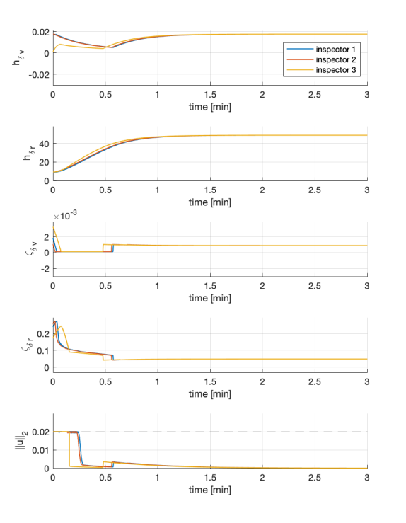
Figure 2: Time evolution of the CBFs $h_{\delta\bm{v}}$,$h_{\delta\bm{r}}$; the HOCBF nominal function $\zeta_{\delta\bm{r}}$,$\zeta_{\delta\bm{v}}$; and the control signal $\|\bm{u}\|_{2}$ for each inspector.

VII CONCLUSIONS AND FUTURE WORK

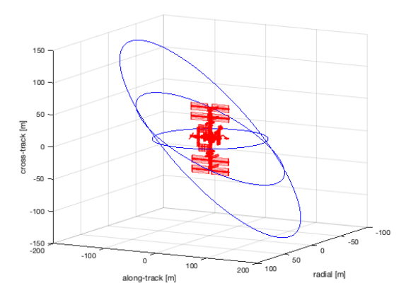
Figure 3: Three PRO assigned to each inspector around the ISS. The base directions are given in terms of the LVLH frame where $\hat{\bm{r}}$ is the radial direction, $\hat{\bm{s}}$ is the along-track direction and $\hat{\bm{w}}$ is the cross-track direction.

In this work, we developed new definitions of sampled-data HOCBF thanks to which continuous-time safety guarantees can be ensured for sampled-data high-order systems. Then, we explored the applicability of the CMPC with the newly introduced definition of SD-HOCBF for a realistic space mission scenario. In future work, we will investigate how to determine suitable parameters for the CMPC scheme in a programmatic manner and we will analyse the impact of sensor noise on the control performance.

References

• [1] A. Dorri, S. S. Kanhere, and R. Jurdak, “Multi-Agent Systems: A Survey,” IEEE Access, vol. 6, pp. 28 573–28 593, 2018.
• [2] M. Mesbahi and M. Egerstedt, “Graph theoretic methods in multiagent networks,” in Graph Theoretic Methods in Multiagent Networks.   Princeton University Press, 2010.
• [3] A. Ekblaw and J. Paradiso, “Self-Assembling Space Habitats: TESSERAE design and mission architecture,” in Aerospace Conference.   IEEE, 2019, pp. 1–11.
• [4] B. Khoshnevis, A. Carlson, and M. Thangavelu, “ISRU-based robotic construction technologies for lunar and martian infrastructures,” Tech. Rep., 2017.
• [5] A. Flores-Abad, O. Ma, K. Pham, and S. Ulrich, “A review of space robotics technologies for on-orbit servicing,” Progress in Aerospace Sciences, vol. 68, pp. 1–26, Jul. 2014.
• [6] Y. K. Nakka, W. Hönig, C. Choi, A. Harvard, A. Rahmani, and S.-J. Chung, “Information-based guidance and control architecture for multi-spacecraft on-orbit inspection,” Journal of Guidance, Control, and Dynamics, vol. 45, no. 7, pp. 1184–1201, 2022.
• [7] K. T. Alfriend, S. R. Vadali, P. Gurfil, J. P. How, and L. Breger, Spacecraft formation flying: Dynamics, control and navigation.   Elsevier, 2009, vol. 2.
• [8] J. Zeng, B. Zhang, and K. Sreenath, “Safety-critical model predictive control with discrete-time control barrier function,” in American Control Conference (ACC).   IEEE, 2021, pp. 3882–3889.
• [9] W. S. Cortez, D. Oetomo, C. Manzie, and P. Choong, “Control barrier functions for mechanical systems: Theory and application to robotic grasping,” IEEE Transactions on Control Systems Technology, vol. 29, no. 2, pp. 530–545, 2019.
• [10] J. Breeden, K. Garg, and D. Panagou, “Control barrier functions in sampled-data systems,” IEEE Control Systems Letters, vol. 6, pp. 367–372, 2021.
• [11] P. Roque, W. S. Cortez, L. Lindemann, and D. V. Dimarogonas, “Corridor MPC: Towards optimal and safe trajectory tracking,” in American Control Conference (ACC).   IEEE, 2022, pp. 2025–2032.
• [12] X. Tan and D. V. Dimarogonas, “Compatibility checking of multiple control barrier functions for input constrained systems,” in Conference on Decision and Control (CDC).   IEEE, 2022, pp. 939–944.
• [13] D. Morgan, S.-J. Chung, L. Blackmore, B. Acikmese, D. Bayard, and F. Y. Hadaegh, “Swarm-keeping strategies for spacecraft under J2 and atmospheric drag perturbations,” Journal of Guidance, Control, and Dynamics, vol. 35, no. 5, pp. 1492–1506, 2012.
• [14] A. D. Ames, S. Coogan, M. Egerstedt, G. Notomista, K. Sreenath, and P. Tabuada, “Control barrier functions: Theory and applications,” in European Control Conference (ECC).   IEEE, 2019, pp. 3420–3431.
• [15] W. Xiao and C. Belta, “Control barrier functions for systems with high relative degree,” in Conference on Decision and Control (CDC).   IEEE, 2019, pp. 474–479.
• [16] E. D. Sontag, Mathematical control theory: deterministic finite dimensional systems.   Springer Science & Business Media, 2013, vol. 6.
• [17] S. Scholtes, Introduction to piecewise differentiable equations.   Springer Science & Business Media, 2012.