tinyBenchmarks: evaluating LLMs with fewer examples

Abstract

The versatility of large language models (LLMs) led to the creation of diverse benchmarks that thoroughly test a variety of language models’ abilities. These benchmarks consist of tens of thousands of examples making evaluation of LLMs very expensive. In this paper, we investigate strategies to reduce the number of evaluations needed to assess the performance of an LLM on several key benchmarks. For example, we show that to accurately estimate the performance of an LLM on MMLU, a popular multiple-choice QA benchmark consisting of 14K examples, it is sufficient to evaluate this LLM on 100 curated examples. We release evaluation tools and tiny versions of popular benchmarks: Open LLM Leaderboard, MMLU, HELM, and AlpacaEval 2.0. Our empirical analysis demonstrates that these tools and tiny benchmarks are sufficient to reliably and efficiently reproduce the original evaluation results.

1 Introduction

Large Language Models (LLMs) have demonstrated remarkable abilities to solve a diverse range of tasks (Brown et al., 2020). Quantifying these abilities and comparing different LLMs became a challenge that led to the development of several key benchmarks, e.g., MMLU (Hendrycks et al., 2020), Open LLM Leaderboard (Beeching et al., 2023), HELM (Liang et al., 2022), and AlpacaEval (Li et al., 2023).

These benchmarks are comprised of hundreds or thousands of examples, making the evaluation of modern LLMs with billions of parameters computationally, environmentally, and financially very costly. For example, Liang et al. (2022) report that evaluating the performance of a single LLM on HELM costs over 4K GPU hours (or over $10K for APIs). Benchmarks like AlpacaEval (Li et al., 2023) also require a commercial LLM as a judge to perform evaluation, further increasing the costs. Furthermore, evaluation of a single model is often performed many times to monitor checkpoints during pre-training (Biderman et al., 2023a; Liu et al., 2023) and to explore different prompting strategies or a wider range of hyperparameters (Weber et al., 2023b; Mizrahi et al., 2023; Sclar et al., 2023; Voronov et al., 2024).

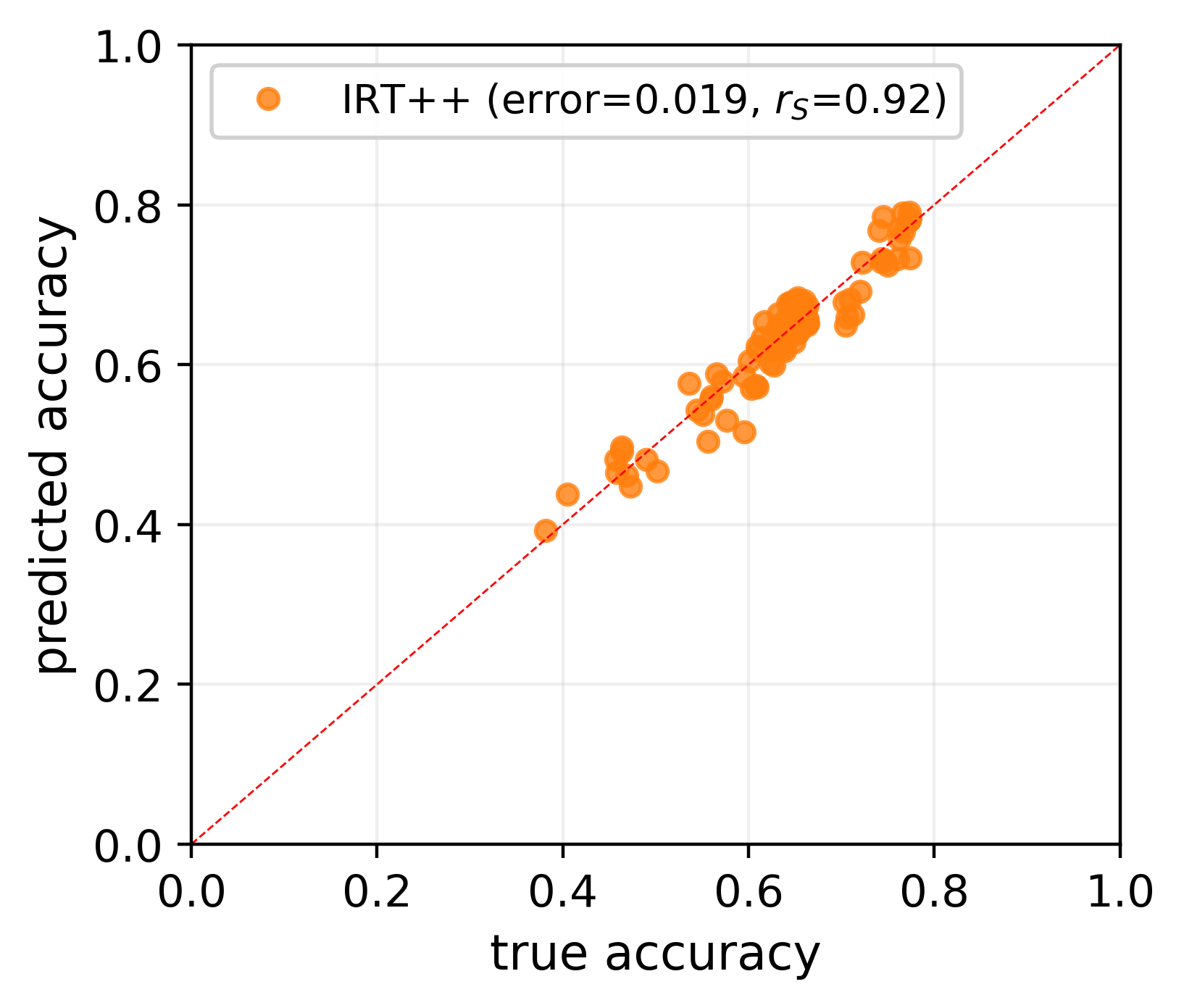
Figure 1: Estimating accuracy on MMLU (true accuracy) using 100 curated examples (predicted accuracy). IRT++, our best-performing evaluation strategy, predicts the accuracy of recent LLMs released between December 30th and January 18th within 1.9% of their true accuracy on all of MMLU (14K examples).

Our work reassesses the need to evaluate LLMs on such large benchmark datasets. In Figure 1 we demonstrate the efficacy of our best evaluation strategy on MMLU, where we compare accuracy estimates obtained from evaluating LLMs on a curated subset of 100 examples (less than 1% of the examples) to accuracy on all of MMLU, achieving average estimation error under 2%.

We consider a range of evaluation strategies (§3):

1. Stratified random sampling as proposed by Perlitz et al. (2023) for HELM. This approach is the simplest to use but can result in a large estimation error.

2. Clustering examples based on LLMs that have already been evaluated. The key idea is to find examples where (in)correct prediction of an LLM implies that it will also be (in)correct on a subset of other examples. This method performs well in some settings but can be unreliable when such correctness patterns are spurious, e.g., when predicting the accuracy of an LLM specialized to a domain. This strategy is inspired by the Anchor Points method (Vivek et al., 2023) which clusters models’ confidence in the correct class for faster evaluation on classification tasks.

3. New strategies built using Item Response Theory (IRT) (Lord et al., 1968) for evaluating individuals through standardized tests. Applying IRT to LLMs viewed as testees and benchmarks as tests, we learn representations of examples encoding latent abilities required to perform well on these examples. Clustering these representations allows us to find a more robust evaluation set. Furthermore, using the IRT model, we develop tools for improving benchmark accuracy estimates obtained with an arbitrary set of examples.

We present an extensive evaluation of these strategies on four popular benchmarks (§5): Open LLM Leaderboard (Beeching et al., 2023), MMLU (Hendrycks et al., 2020), HELM (Liang et al., 2022), and AlpacaEval 2.0 (Li et al., 2023). Our goal is to assess the effectiveness of estimating the performance of LLMs on these benchmarks using a limited number of examples for evaluation. Overall, we conclude that 100 curated examples per scenario are enough to reliably estimate the performance of various LLMs, within about 2% error on average. Based on our findings we release tiny (100 examples per scenario) versions of every considered benchmark and IRT-based tools for further improving the performance estimation.

1.1 Related work

Efficient benchmarking of LLMs

Multi-dataset benchmarks were introduced to the field of NLP with the advent of pre-trained models (e.g. Wang et al., 2018), and constantly evolved in lockstep with language model capabilities (Srivastava et al., 2022). The ever-increasing size of models and datasets consequently led to high evaluation costs, triggering changes in reported evaluation to accommodate the costs (Biderman et al., 2023b). Ye et al. (2023) considered reducing the number of tasks in Big-bench (Srivastava et al., 2022). Perlitz et al. (2023) found that evaluation on HELM (Liang et al., 2022) relies on diversity across datasets, but the number of examples currently used is excessive. We adopt their stratified sampling approach as one of the efficient evaluation strategies. Vivek et al. (2023) proposed clustering evaluation examples based on models’ confidence in the correct class for faster evaluation on classification tasks. One of the approaches we consider is based on an adaptation of their method to popular LLM benchmarks with more diverse tasks.

Item response theory (IRT)

IRT (Cai et al., 2016; Van der Linden, 2018; Brzezińska, 2020; Lord et al., 1968) is a well-established set of statistical models used in psychometrics to measure the latent abilities of individuals through standardized testing (An & Yung, 2014; Kingston & Dorans, 1982; Petersen et al., 1982), e.g., in GRE, SAT, etc.. Even though IRT methods have been traditionally used in psychometrics, they are becoming increasingly popular among researchers in the fields of artificial intelligence and natural language processing (NLP). For instance, Lalor et al. (2016) propose using IRT’s latent variables to measure language model abilities, Vania et al. (2021) employs IRT models in the context of language models benchmarking to study saturation (un-discriminability) of commonly used benchmarks, and Rodriguez et al. (2021) study several applications of IRT in the context of language models, suggesting that IRT models can be reliably used to: predict responses of LLMs in unseen items, categorize items (e.g., according to their difficulty/discriminability), and rank models. However, to the best of our knowledge, IRT has not been used for performance estimation in the context of efficient benchmarking of LLMs. We explore this new path.

Active testing

Another line of related work is related to active learning (Ein-Dor et al., 2020) and especially active testing. In such works, evaluation examples are chosen dynamically using various criteria (Ji et al., 2021; Kossen et al., 2021) to minimize annotation costs. Those methods are somewhat similar to the adaptive IRT which we discuss in §6.

2 Problem statement

In this section, we describe in detail the setup we work on and what are our objectives. Consider that a benchmark is composed of scenarios and possibly sub-scenarios. For example, MMLU and GSM8K are examples of scenarios of both the Open LLM Leaderboard and HELM (Lite), while MMLU has different sub-scenarios like “marketing”, “elementary mathematics”, and so on. Furthermore, each scenario (or sub-scenario) is composed of examples (analogous to “items” in the IRT literature) that are small tests to be solved by the LLMs–these examples range from multiple-choice questions to text summarization tasks. Our final objective is to estimate the performance of LLMs in the full benchmark, which is given by the average of the performances in individual scenarios (Open LLM Leaderboard, MMLU, AlpacaEval 2.0) or mean-win-rate (HELM). We achieve this objective by first estimating the performance of LLMs in individual scenarios and then aggregating scores. When scenarios have sub-scenarios, it is usually the case that the scenario performance is given by a simple average of sub-scenarios performances. The main concern is that each scenario/sub-scenario is composed of hundreds or thousands of examples, making model evaluation costly.

In this work, for a fixed benchmark, we denote the set of examples of each scenario $j$ as $\mathcal{I}_{j}$, implying that the totality of examples in the benchmark is given by $\mathcal{I}=\cup_{j}\mathcal{I}_{j}$. When an LLM $l$ interacts with an example $i\in\mathcal{I}_{j}$, the system behind the benchmarks generates a score that we call “correctness” and denote as $Y_{il}$. In all the benchmarks we consider in this work, the correctness is either binary, i.e., $Y_{il}\in\{0,1\}$ (incorrect/correct), or bounded, i.e., $Y_{il}\in[0,1]$, denoting a degree of correctness. The second case is applied in situations in which, for instance, there might not be just one correct answer for example $i$. To simplify the exposition in the main text, we assume that the score for LLM $l$ in scenario $j$ is just the simple average of the correctness of all items in that scenario, that is, $\frac{1}{|\mathcal{I}_{j}|}\sum_{i\in\mathcal{I}_{j}}Y_{il}$. That is not true when different sub-scenarios have different numbers of examples; in that case, one would just have to use a weighted average instead, to make sure every sub-scenario is equally important (in the experiments, we consider this case). In Appendix A, we explain in more detail how things change when a scenario has subscenarios with different sizes but we want to give the same importance to each one of them. Our objective when evaluating a model $l$ is to choose a small fraction of examples $\widehat{\mathcal{I}}_{j}\subset\mathcal{I}_{j}$, compute the correctness of model $l$ in every example of $\widehat{\mathcal{I}}_{j}$, and then use the available data to estimate what would be the average score of that model in $\mathcal{I}_{j}$, i.e., $\frac{1}{|\mathcal{I}_{j}|}\sum_{i\in\mathcal{I}_{j}}Y_{il}$. In the next section, we describe strategies on how $\widehat{\mathcal{I}}_{j}$ can be chosen and how the overall score can be estimated.

3 Selecting evaluation examples

In this section, we describe strategies on how to select examples from a fixed scenario $j$, i.e., $\mathcal{I}_{j}$, obtaining $\widehat{\mathcal{I}}_{j}\subset\mathcal{I}_{j}$ described in Section 2. Ideally, the set of selected examples should be representative of the whole set of items in scenario $j$, that is,

$$\textstyle\sum_{i\in\widehat{\mathcal{I}}_{j}}w_{i}Y_{il}\approx\frac{1}{|\mathcal{I}_{j}|}\sum_{i\in\mathcal{I}_{j}}Y_{il},$$ (3.1)

for nonnegative weights $\{w_{i}\}_{i\in\widehat{\mathcal{I}}_{j}}$ such that $\sum_{i\in\widehat{\mathcal{I}}_{j}}w_{i}=1$. In the next paragraphs, we describe two possible ways of obtaining $\widehat{\mathcal{I}}_{j}$ and $\{w_{i}\}_{i\in\widehat{\mathcal{I}}_{j}}$.

3.1 Stratified random sampling

In some settings (e.g., classifiers Katariya et al., 2012), it is useful to perform stratified random sampling – subsample examples ensuring the representation of certain groups of data. Using subscenarios as the strata for stratified random sampling was proposed by Perlitz et al. (2023) when sub-sampling examples from HELM scenarios. The authors showed that this is an effective way of sampling examples without too much loss on the ability to rank LLMs by performance. Examples should be randomly selected from sub-scenarios (with uniform probability) in a way such that the difference in number of examples sampled for two distinct subscenarios is minimal ($\leq 1$). The rationale behind this method is that, for an effective evaluation, sub-scenarios should be equally represented. The weights are $w_{i}=1/|\widehat{\mathcal{I}}_{j}|$ for all $i\in\widehat{\mathcal{I}}_{j}$.

3.2 Clustering

Assessing the performance of LLM’s on a randomly sampled subset of examples suffers from extra uncertainty in the sampling process, especially when the number of sampled examples is small. Instead, we consider selecting a subset of representative examples using clustering. Vivek et al. (2023) proposed to cluster examples based on the confidence of models in the correct class corresponding to these examples. Representative examples, from these clusters, which they call “anchor points”, can then be used to evaluate models on classification tasks more efficiently. We adapt their clustering approach to a more general setting, allowing us to extract such anchor points for MMLU, AlpacaEval 2.0, and all scenarios of the Open LLM Leaderboard and HELM.

First, we propose to group examples by model correctness, expecting some examples would represent the rest. Ideally, if example $i$ is an anchor point, then there will be a big set of examples on which models are correct if and only if they get example $i$ correct. The same idea applies when correctness is given by a number in $[0,1]$. Assume that we want to select $K$ anchor points and have access to the training set $\mathcal{D}_{tr}=\{Y_{l}\}_{l\in\mathcal{L}_{tr}}$, where $Y_{l}$ is a vector in which each entry is given by the correctness score $Y_{il}$ for all examples $i\in\mathcal{I}_{j}$. We represent each example $i\in\mathcal{I}_{j}$ by the embedding $E_{i}\in{\mathbb{R}}^{|\mathcal{L}_{tr}|}$ which is a vector with entries given by $Y_{il}$ for $l\in\mathcal{L}_{tr}$, and then run $K$-Means (Hastie et al., 2009) with the number of clusters being equal $K$. After the $K$ centroids are obtained, we find the closest example to each centroid, and each of those points will compose $\widehat{\mathcal{I}}_{j}$. For a new LLM $l\not\in\mathcal{L}_{tr}$ to be evaluated, we can obtain an estimate for its performance using the estimate in equation 3.1 by setting $w_{i}$ as the fraction of points in $\mathcal{I}_{j}$ assigned to cluster/anchor point $i$. This method is compelling and simple in detecting anchor points. Still, it can suffer from distribution shifts since correctness patterns can vary, e.g., in time, and from the curse of dimensionality when $|\mathcal{L}_{tr}|$ is big. Our second approach is intended to be more robust to those problems.

The second approach we propose is using item response theory (IRT) representation of examples, detailed in Section 4, as our embeddings $E_{i}$. The IRT model creates a meaningful representation for each example $i$ based on their difficulty and the abilities required to respond to those examples correctly. This approach immediately solves the dimensionality problem, since $E_{i}$ is relatively low-dimensional, and potentially alleviates the distribution shift problem if the IRT model reasonably describes the reality and the example representations are stable. As IRT should represent which examples have similar difficulty and require similar abilities, the anchors represent exactly what we looked for. The weight $w_{i}$ is given by the fraction of examples in $\mathcal{I}_{j}$ assigned to cluster/anchor point $i$.

4 Better performance estimation with IRT

In this section, we propose ways of enhancing performance estimates by using IRT models. We start by discussing the case where $Y_{il}\in\{0,1\}$, that is, the $l$ responds to the example $i\in\mathcal{I}$ correctly or not. We later also discuss the case where $Y_{il}\in[0,1]$.

4.1 The IRT model

The two-parameter multidimensional IRT model assumes that the probability of the LLM $j$ getting example $i$ correctly is given by

$$\textstyle p_{il} \textstyle\triangleq{\mathbb{P}}(Y_{il}=1\mid\theta_{l},\alpha_{i},\beta_{i})=\frac{1}{1+\mathrm{exp}(-\alpha_{i}^{\top}\theta_{l}+\beta_{i})},$$ (4.1)

where $\theta_{l}\in{\mathbb{R}}^{d}$ denotes the unobserved abilities of LLM $l$, while $\alpha_{i}\in{\mathbb{R}}^{d}$ dictates which dimensions of $\theta_{l}$ are required from model $l$ to respond to example $i$ correctly. In this formulation, $\beta_{i}\in{\mathbb{R}}$ can be viewed as a bias term that regulates the probability of correctness when $\theta_{l}=0$. We use IRT parameter estimates as example representations referred to in Section 3. Specifically, we take $E_{i}=(\widehat{\alpha}_{i},\widehat{\beta}_{i})$, where $\widehat{\alpha}_{i}$ and $\widehat{\beta}_{i}$ are point estimates for the parameters of example $i$. In the next sections, we introduce two estimators for the performance of an LLM, propose a simple solution for the case $Y_{il}\not\in\{0,1\}$, and describe model fitting.

4.2 IRT-based LLM performance estimation

The performance-IRT (p-IRT) estimator.

Assume that we are interested in estimating the performance of a model $l\not\in\mathcal{L}_{tr}$ on scenario $j$ and that point estimates of example parameters, $(\widehat{\alpha}_{i},\widehat{\beta}_{i})$, have been computed, using a training set, for all examples in all scenarios, including examples $i\in\mathcal{I}_{j}$. Formally, we are interested in approximating

$$\textstyle Z_{jl}\triangleq\frac{1}{|\mathcal{I}_{j}|}\sum_{i\in\mathcal{I}_{j}}Y_{il}$$ (4.2)

Now, assume that we have run model $l$ on a subset of examples from scenario $j$, obtaining responses $\{Y_{i_{0}l},\cdots,Y_{i_{k}l}\}$ for the examples $\widehat{\mathcal{I}}_{j}=\{i_{0},\cdots,i_{k}\}$. Let $\widehat{\theta}_{l}$ denote the estimate for $\theta_{l}$ after observing $\widehat{\mathcal{I}}_{j}$ and possibly a bigger set of examples coming from different scenarios. To obtain that estimate, we maximize the log-likelihood of the freshly observed data with respect to $\theta_{l}$, fixing examples’ parameters. This procedure is equivalent to fitting a logistic regression model, which is an instance of the well-studied $M$-estimation procedure.

Because $Z_{jl}$ is a random variable, we approximate it by estimating the conditional expectation

$$\textstyle{\mathbb{E}}[Z_{jl}\mid Y_{i_{0}l},\cdots,Y_{i_{k}l}]=$$

$$\textstyle=\frac{1}{|{\mathcal{I}}_{j}|}\sum_{i\in{\mathcal{I}}_{j}}{\mathbb{E}}[Y_{il}\mid Y_{i_{0}l},\cdots,Y_{i_{k}l}]$$

$$\textstyle=\frac{1}{|{\mathcal{I}}_{j}|}\left(\sum_{i\in\widehat{\mathcal{I}}_{j}}Y_{il}+\sum_{i\in{\mathcal{I}}_{j}\setminus\widehat{\mathcal{I}}_{j}}p_{il}\right)$$

$$\textstyle=\frac{\hat{\lambda}}{|\widehat{\mathcal{I}}_{j}|}\sum_{i\in\widehat{\mathcal{I}}_{j}}Y_{il}+\frac{1-\hat{\lambda}}{|{\mathcal{I}}_{j}\setminus\widehat{\mathcal{I}}_{j}|}\sum_{i\in{\mathcal{I}}_{j}\setminus\widehat{\mathcal{I}}_{j}}p_{il}$$

where $\hat{\lambda}=|\widehat{\mathcal{I}}_{j}|/|{\mathcal{I}}_{j}|\in[0,1]$ is a weight that gives more or less importance to the observed set $\widehat{\mathcal{I}}_{j}$ in the performance computation depending on how big that set is. The probability $p_{il}={\mathbb{P}}(Y_{il}=1\mid\theta_{l},\alpha_{i},\beta_{i})$ is given by the IRT model in Equation 4.1. The estimator for the conditional expectation is then given by

$$\textstyle\hat{Z}^{\text{p-IRT}}_{jl} \textstyle\triangleq\widehat{{\mathbb{E}}}[Z_{jl}\mid Y_{i_{0}l},\cdots,Y_{i_{k}l}]$$ (4.3)

$$\textstyle=\frac{\hat{\lambda}}{|\widehat{\mathcal{I}}_{j}|}\sum_{i\in\widehat{\mathcal{I}}_{j}}Y_{il}+\frac{1-\hat{\lambda}}{|{\mathcal{I}}_{j}\setminus\widehat{\mathcal{I}}_{j}|}\sum_{i\in{\mathcal{I}}_{j}\setminus\widehat{\mathcal{I}}_{j}}\hat{p}_{il}$$

where $\hat{p}_{il}\triangleq{\mathbb{P}}(Y_{il}=1\mid\widehat{\theta}_{l},\widehat{\alpha}_{i},\widehat{\beta}_{i})$. We call the estimator in 4.3 by Performance-IRT (p-IRT) estimator.

The idea behind p-IRT is that we can estimate the performance of a model on unseen data making use of the IRT model. This is especially useful if we can fit $\widehat{\theta}_{l}$ using data from many scenarios: even though we observe just a few samples per scenario, p-IRT will leverage the whole available data, permitting better estimates for the performance of the LLM for all scenarios. Conditional on the training set, the estimator p-IRT has low variance when $\widehat{\theta}_{l}$ is obtained from a large dataset and a small bias if the IRT model is reasonably specified. Given that $\widehat{\theta}_{l}$ is potentially estimated using a large sample, it is worth understanding what that implies about our estimates $\hat{p}_{il}$’s in the asymptotic regime. To facilitate our analysis, assume for a moment that the true values of $(\alpha_{i},\beta_{i})$’s for all $i\in\mathcal{I}$ are known. From the theory of parametric $M$-estimation (Van der Vaart, 2000), under some regularity conditions, we have that $|\widehat{\mathcal{I}}|^{1/2}(\widehat{\theta}_{l}-\theta^{*}_{l})\overset{d}{\to}N(0,A_{l})$ as $|\widehat{\mathcal{I}}|\to\infty$ for a certain covariance matrix $A_{l}$, where $\theta^{*}_{l}$ denotes the true ability parameter for LLM $l$ and $\widehat{\mathcal{I}}=\cup_{j}\widehat{\mathcal{I}}_{j}$. Using the delta method (Van der Vaart, 2000), we affirm in Proposition 4.1 that $\hat{p}_{il}$ is asymptotically normal and centered around $p_{il}$:

Proposition 4.1.

Assuming that the true values of $(\alpha_{i},\beta_{i})$’s for all $i\in\mathcal{I}$ are known and under standard $M$-estimation regularity conditions, by the delta method,

$$|\widehat{\mathcal{I}}|^{1/2}(\widehat{p}_{il}-p_{il})\overset{d}{\to}N(0,(\sigma^{\prime}(-\alpha_{i}^{\top}\theta+\beta_{i}))^{2}\alpha_{i}^{\top}A_{l}\alpha_{i}),$$

where $\sigma$ is the logistic regression link function.

Proposition 4.1 implies that $\hat{p}_{il}=p_{il}+\mathcal{O}_{P}(|\widehat{\mathcal{I}}|^{-1/2})$, meaning that $p_{il}$ can be accurately estimated when $|\widehat{\mathcal{I}}|$ is large. Consequently, the performance can be well approximated in this setup.

We note two limitations of p-IRT that can hinder its effectiveness in practice. First, it does not promptly allow sample weighting, limiting its use of anchor points; second, if the predicted probabilities $\hat{p}_{il}$’s are inaccurate, e.g., because of model misspecification, then the performance of p-IRT will deteriorate.

The generalized p-IRT (gp-IRT) estimator.

Our final estimator builds upon p-IRT to overcome its limitations. Assume that the estimators in equations 3.1 and 4.3 are obtained as a first step after the collection of examples in $\widehat{\mathcal{I}}_{j}$. The idea is to compute a third estimator $\hat{Z}^{\text{gp-IRT}}_{jl}$ given by a convex combination of the first two

$$\textstyle\hat{Z}^{\text{gp-IRT}}_{jl}\triangleq\lambda\sum_{i\in\widehat{\mathcal{I}}_{j}}w_{i}Y_{il}+(1-\lambda)\hat{Z}^{\text{p-IRT}}_{jl}$$ (4.4)

where $\lambda$ is a number in $[0,1]$ that is chosen to optimize the performance of that estimator. To choose $\lambda$, we first note that using random sampling (or anchor points) implies low bias but potentially high variance (when $\widehat{\mathcal{I}}_{j}$ is small) for $\sum_{i\in\widehat{\mathcal{I}}_{j}}w_{i}Y_{il}$. As $\widehat{\mathcal{I}}_{j}$ grows, its variance decreases. On the other hand, conditional on the training set, the variance of $\hat{Z}^{\text{p-IRT}}_{jl}$ is small, especially when $\widehat{\theta}_{l}$ is fitted with data from many scenarios, but its bias can be high when the IRT model is misspecified and does not vanish with the growing sample size. Thus, good choice of $\lambda$ increases with $\widehat{\mathcal{I}}_{j}$.

We choose $\lambda$ based on a heuristic derived from Song (1988)’s Corollary 2. It tells us that the optimal linear combination of any two estimators $\hat{T}_{1}$ and $\hat{T}_{2}$ (when the sum of the weights is one) depends on the biases, variances, and covariance of the two estimators. If the first estimator is unbiased and the variance of the second is zero, we can show that the optimal estimator is $\lambda\hat{T}_{1}+(1-\lambda)\hat{T}_{2}$, where $\lambda=b^{2}_{2}/(b^{2}_{2}+v_{1})$, $b_{2}$ denotes $\hat{T}_{2}$’s bias, and $v_{1}$ denotes $\hat{T}_{1}$’s variance. To apply this result, we assume that the main factors that might prevent gp-IRT from being a good estimator are the variance of the first estimator and the bias of the second one. Then we approximate the first estimator’s bias and the second estimator’s variance by zero. When our first estimator is obtained by random sampling we take

$$\lambda=\frac{\hat{b}^{2}}{\hat{\sigma}^{2}/|\widehat{\mathcal{I}}_{j}|+\hat{b}^{2}}$$

for two constants $\hat{\sigma}^{2}$ and $\hat{b}^{2}$. The first constant, $\hat{\sigma}^{2}$, is obtained by computing the average sample variance of $Y_{il}$, $i\in\mathcal{I}_{j}$, across LLMs in the training set. The second constant, $\hat{b}^{2}$, is obtained by approximating the IRT bias. We (i) split the training set into two subsets of LLMs; (ii) fit an IRT model in the first part using data from all scenarios; (iii) fit the ability parameter for all the LLMs in the second part using half of the examples of all scenarios; (iv) use that IRT model to predict the correctness (using predicted probabilities) of the unseen examples of scenario $j$ for the models in the second split; (v) average predictions and actual correctness within models, obtaining predicted/actual scenarios scores; (vi) compute their absolute differences, obtaining individual error estimates for models; (vii) average between models, obtaining a final bias estimate, and then square the final number. To give some intuition on how $\lambda$ is assigned, Figure 2 depicts $\lambda$ as a function of $\hat{b}$ and $|\widehat{\mathcal{I}}_{j}|$ when $\hat{\sigma}^{2}=.01$. From that figure, we see that if the IRT model bias is small, more weight will be given to p-IRT. The curves are steeper when $|\widehat{\mathcal{I}}_{j}|$ is small because the variance of the first estimator decreases faster when $|\widehat{\mathcal{I}}_{j}|$ is small.

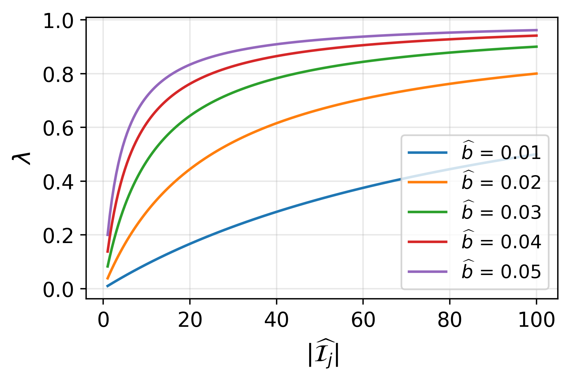
Figure 2: Understanding the effect of IRT bias and sample size $|\widehat{\mathcal{I}}_{j}|$ in the gp-IRT construction: both quantities are positively related to the weight we give to the raw data in performance estimation.

When the first estimator is obtained by a method that implies an estimator with smaller variance, e.g., anchor points, we apply the same formula but divide $\hat{\sigma}^{2}$ by a constant $>1$. By default, we divide $\hat{\sigma}^{2}$ by $4$ which is equivalent to halving the standard deviation of the first estimator.

4.3 Using IRT when $Y_{il}$ is not binary

There are situations in which $Y_{il}\notin\{0,1\}$ but $Y_{il}\in[0,1]$. For example, in AlpacaEval 2.0, the response variable is bounded and can be translated to the interval $[0,1]$. Also, some scenarios of HELM and the Open LLM Leaderboard have scores in $[0,1]$. We propose a simple and effective fix. The idea behind our method is to binarize $Y_{il}$ by defining a second variable $\tilde{Y}_{il}=\mathds{1}[Y_{il}\geq c]$, for a scenario-dependent constant $c$. More concretely, for each scenario $j$, we choose $c$ such that

$$\textstyle\sum_{i\in\mathcal{I}_{j},l\in\mathcal{L}_{tr}}Y_{il}\approx\sum_{i\in\mathcal{I}_{j},l\in\mathcal{L}_{tr}}\mathds{1}[Y_{il}\geq c].$$

In that way, approximating the average of $\tilde{Y}_{il}$ and $Y_{il}$ should be more or less equivalent. Given that $\tilde{Y}_{il}\in\{0,1\}$, we can use the standard IRT tools to model it.

4.4 Fitting the IRT model

For the estimation procedure, we resort to variational inference. In particular, we assume that $\theta_{l}\sim N(\mu_{\theta}\mathds{1}_{d},1/u_{\theta}I_{d})$, $\alpha_{i}\sim N(\mu_{\alpha}\mathds{1}_{d},1/u_{\alpha}I_{d})$, and $\beta_{i}\sim N(\mu_{\beta},1/u_{\beta})$. To take advantage of software for fitting hierarchical Bayesian models (Lalor & Rodriguez, 2023), we introduce (hyper)priors for the prior parameters $\mu_{\theta}\sim N(0,10)$, $u_{\theta}\sim\Gamma(1,1)$, $\mu_{\alpha}\sim N(0,10)$, $u_{\alpha}\sim\Gamma(1,1)$, $\mu_{\beta}\sim N(0,10)$, and $u_{\beta}\sim\Gamma(1,1)$. Finally, to obtain point estimates for the model and example-specific parameters $\theta_{l}$, $\alpha_{i}$, and $\beta_{i}$, we use the means of their variational distributions. To select the dimension of the IRT model during the fitting procedure, we run a simple validation strategy in the training set and choose the dimension that maximizes the prediction power of the IRT model in the validation split–we consider the dimensions in $\{2,5,10,15\}$.

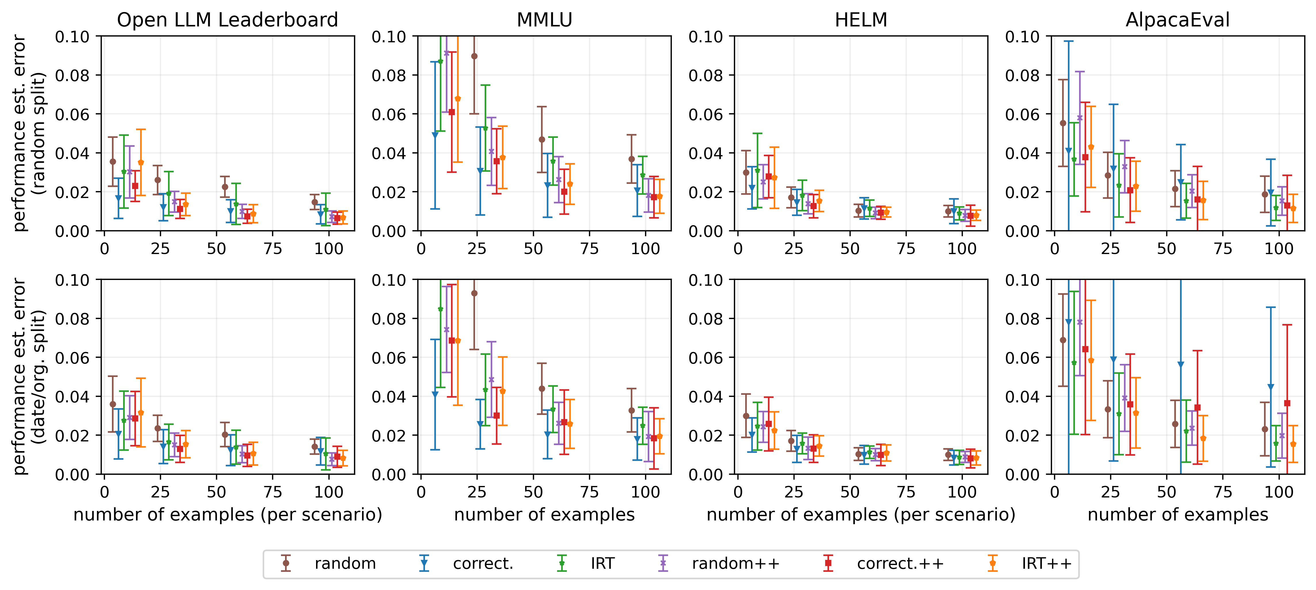
Figure 3: Performance estimation error per benchmark (columns) tested on random (top row) and recent (bottom row) LLMs for increasing number of evaluation examples. 100 examples per scenario is sufficient to achieve $\approx$2% average performance estimation error across benchmarks and evaluated LLMs. This corresponds to 600 out of 29K examples for Open LLM Leaderboard, 100 out of 14K examples for MMLU, 1000 out of 10K examples for HELM, and 100 out of 800 examples for AlpacaEval 2.0.

5 Assessing evaluation strategies

We assess the ability of the considered evaluation strategies to estimate the performance of LLMs on four popular benchmarks. For a given LLM and a benchmark, each evaluation strategy estimates the performance using evaluation results of this LLM on a given number of examples. We then compare this estimate to the true value, i.e., the performance of this LLM on the complete benchmark.

We use publicly available evaluation data for which we split the models into “train” and “test”. Evaluation of the train models is used to find the anchor points and fit the IRT model. The ability to predict performance is measured on the test set of models. We consider two train-test split scenarios: (i) random split and (ii) by date, i.e. using the most recent models for testing. The latter split better represents practical use cases, while also being more challenging as it is likely to result in a distribution shift between the train and test models due to improving model capabilities over time that might affect the effectiveness of anchor points and the IRT model.

Benchmarks and models

We describe the size and composition of the four benchmarks, as well as the corresponding LLMs (see Appendix C for additional details):

• HuggingFace’s Open LLM Leaderboard (Beeching et al., 2023) consists of 6 scenarios, approx. 29K examples in total. Performance on each of the scenarios is measured with accuracy and the overall benchmark performance is equal to the average of scenario accuracies. We collect evaluation results for 395 LLMs from the Leaderboard’s website and use 75% for training and 25% for testing (split either randomly or by date as described above).

• MMLU (Hendrycks et al., 2020) is a multiple choice QA scenario consisting of 57 subjects (subscenarios) comprising approx. 14K examples. Performance on MMLU is measured by averaging the accuracies on each of the categories. MMLU is one of the 6 scenarios of the Open LLM Leaderboard and we consider the same set of 395 LLMs and train-test splits. The reason to consider it separately is its immense popularity when comparing LLMs (Touvron et al., 2023; Achiam et al., 2023; Team et al., 2023) and inclusion into several other benchmarks.

• For HELM (Liang et al., 2022), we use HELM Lite v1.0.0, which has the 10 core scenarios (total of approx. 10K evaluation examples) and 30 models that have their performances registered for all scenarios. Performance metrics for each scenario vary and can be non-binary (e.g., F1 score), and the overall performance on the benchmark is measured with mean win rate across scenarios. For this benchmark, the dates models were added are not available. Instead, we split models based on the organizations that trained them to create more challenging train-test splits, e.g., all OpenAI models are either in train or in test. For the random train-test split we use 11-fold cross-validation.

• AlpacaEval 2.0 (Li et al., 2023) consists of 100 LLMs evaluated on 805 examples. Although it is a fairly small benchmark, evaluation is expensive as it requires GPT-4 as a judge. For each input, GPT-4 compares the responses of a candidate LLM and a baseline LLM (currently also GPT-4) and declares a winner. The average win rate is used to measure the overall performance. When splitting the data by date, we pick $25\%$ most recent models for testing and the rest for training. For the random split, we employ 4-fold cross-validation.

Evaluation strategies

We consider 3 strategies presented in §3 for selecting a subset of examples for efficient evaluation: “random” for stratified random sampling, “correctness” for clustering correctness of models in the train set, and “IRT” for clustering the example representations obtained from the IRT model fit on the train set. For each strategy, we evaluate the vanilla variation, i.e., simply using the performance of a test LLM on the (weighted) set of selected examples to estimate its performance on the full benchmark, and “++” variation that adjusts this estimate using the IRT model as described in equation (4.4). In total, we assess six evaluation strategies. Results are averaged over 5 restarts.

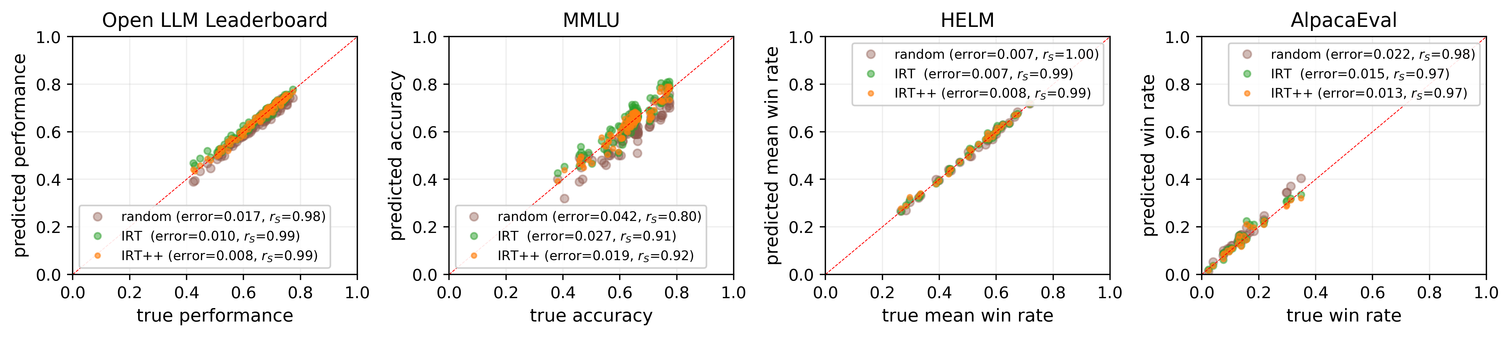
Figure 4: Predicted performance compared with true performance for the four benchmarks (columns) and recent LLMs. We verify the efficacy of the evaluation strategies (IRT and IRT++) we chose to construct tinyBenchmarks.

Key findings

We investigate the effectiveness of strategies as we increase the number of examples available for evaluating test LLMs. Results for both train-test split scenarios are presented in Figure 3 (see also Figure 12 for Spearman’s rank correlations). Our main conclusions are:

• Our approach to reducing evaluation costs is effective. The best-performing strategies achieve estimation error within 2% on all benchmarks with 100 examples or less per dataset or scenario. For example, for MMLU this reduces the evaluation cost by a factor of 140 (from 14k to 100). For Open LLM Leaderboard even 30 examples per scenario is enough, reducing the evaluation cost by a factor of 160 (from 29K to 180).

• Most strategies perform well when there is a temporal shift between the train and test LLM’s (see the lower row of plots in Figure 3 for the results with “by date” split). Thus our approaches for reducing evaluation costs remain practical when evaluating the performance of newer, more capable LLMs and can help save GPU hours when evaluating future LLMs and/or checkpoints during pre-training.

• IRT-based methods (“IRT” and “IRT++”) perform consistently well across benchmarks and train-test splits. The gp-IRT (“++”) variation always improves or matches its vanilla counterpart, while adding only a few seconds to the evaluation time (see Figure 11). Thus we use the IRT-based anchor examples to construct tiny versions tiny versions (100 examples per scenario) of each of the benchmarks and release them along with the gp-IRT tool (code and pre-trained IRT model) for efficient evaluation of future LLMs. We present additional evaluations of tinyBenchmarks in Figure 4. In Appendix B, we conduct an exploratory analysis of the examples comprising tinyMMLU.

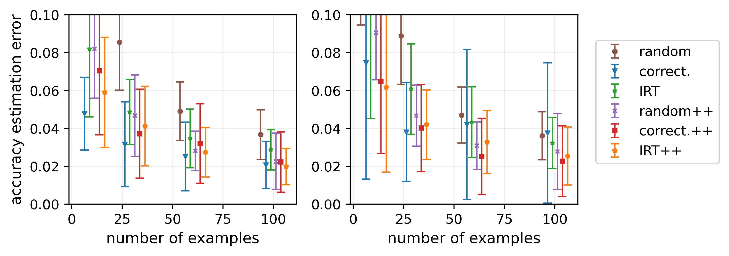
Figure 5: Estimation error on specialized LLMs (right) compared to error on random LLMs (left) on MMLU. Correctness-based example selection is affected the most by this distribution shift.

Specialized LLMs

In our previous experiments the test set of LLMs consisted of either a random subset of models or the most recent ones. Both of these test sets are dominated by base and instruction-tuned LLMs. Here we assess the ability of the considered strategies to predict the performance of specialized LLMs, i.e., models fine-tuned for specific domains such as code, biology, or finance. We consider MMLU benchmark and collect a new hand-picked test set of 40 specialized models. Such models are likely to have unique strengths and perform well in specific MMLU categories while relatively underperforming on others. Thus, their correctness patterns might be different from those in the train set, posing a challenge for our evaluation strategies. We present results in Figure 5.

As we anticipated, the correctness-based anchor strategy deteriorates when tested on specialized LLMs. In contrast to the IRT-based anchors that are only slightly affected, demonstrating their robustness and supporting our choice to use them for tinyBenchmarks construction.

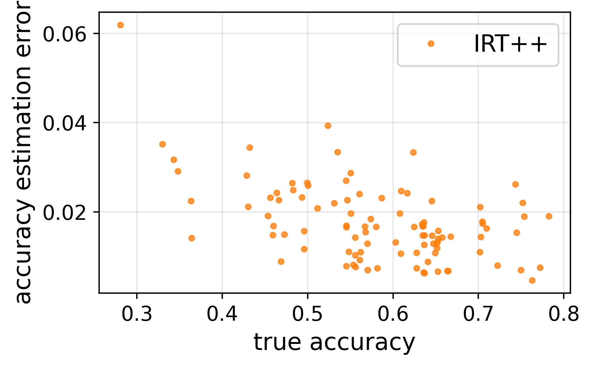
Figure 6: Spread of estimation errors across a random subset of LLMs with varying capabilities on MMLU. The error tends to be slightly lower for more capable models. The worst case error across almost all models is $\leq 4\%$.

Estimation error analysis

We present a more detailed view of the estimation error of the best performing “IRT++” evaluation strategy on MMLU with 100 examples. In Figure 6 we plot estimation error against the actual accuracy of 99 test LLMs for a random train-test split. Our strategy can estimate the performance of more capable LLMs slightly better, although there is no strong dependency. We also note that the estimation error never exceeds 4% (except for one LLM with extremely low performance). Recall that the average error is 2% as shown in Figure 3, supporting the reliability of our evaluation approach.

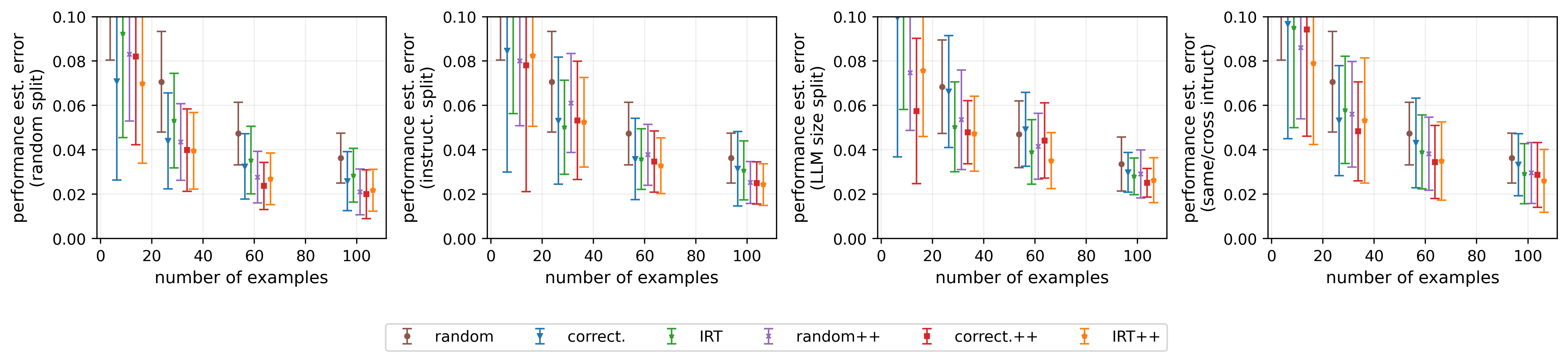
Figure 7: Estimation error when predicting the performance of prompt templates. The results demonstrate that using our methods for efficient prompt-based model evaluation is a promising application.

6 Conclusion

In this paper, we demonstrate it is possible to accurately assess the capabilities of LLMs with a fraction (sometimes two orders of magnitude smaller) of the examples in common benchmark datasets by leveraging models of educational assessments from psychometrics. This leads directly to savings in terms of the monetary costs associated with evaluating LLMs, but also the computational and environmental costs. For practitioners, the computational cost savings are especially convenient because they enable them to evaluate LLMs more frequently during fine-tuning and prompt engineering.

Based on our results we are releasing tinyBenchmarks, pre-selected subsets of examples from the widely adopted LLM benchmarks. tinyBenchmarks are simply small datasets that are straightforward to use to evaluate LLMs cheaply. We are also releasing an IRT-based tool to enhance performance estimation. The tool provides code and IRT parameters trained on the corresponding benchmarks and can be run on a CPU in a few seconds.

6.1 Extensions

Prompt evaluation

A persistent challenge in prompt-based model evaluation is the influence the prompting setup has on model predictions (see, e.g., Lu et al., 2022; Mishra et al., 2022; Min et al., 2022; Yoo et al., 2022; Weber et al., 2023b; Wei et al., 2023). We can use the previously described approaches to make predictions across different prompting setups. This way, we can estimate how well a model will do on a new set of prompts using just a few evaluations, or how a new model will perform on a given prompt. To test this idea, we train an IRT model on the prediction data from Weber et al. (2023a), containing evaluations of eight LLaMA LLMs (vanilla or instruction tuned on the Alpaca self-instruct dataset; Touvron et al., 2023; Taori et al., 2023) for the ANLI dataset (Nie et al., 2020). The dataset consists of evaluations of the 750 data points wrapped with 15 different instruction templates sourced from the promptsource collection (P3; Bach et al., 2022).

Similarly to our previous experiments, we evaluate random splits and splits featuring distribution shifts (across model sizes and different instruction templates). For model size, we put all models with sizes 7B, 13B, and 30B in the training set while the models with size 65B go to the test set. For splits related to prompts templates, we consider two different approaches: first, we conduct a 2-fold cross-validation rotating instruction templates; second, we consider using the same and different instruction templates in the in-context-learning examples and in the input example alternating the strategies in the training and test sets. Results in Figure 7 suggest that prompt-based model evaluation can be efficiently carried out with the methods introduced in this work, even in the presence of several practical distribution shifts.

Adaptive testing

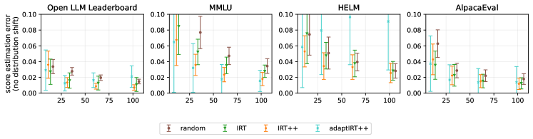
Figure 14: Results of adaptive testing for different benchmarks.

We expect further performance estimation improvements can be squeezed out by more sophisticated applications of similar ideas. For example, instead of pre-selecting a subset of examples before evaluating the LLM, it may be possible to select the examples adaptively during the evaluation process. This idea is widely used in the computerized-assisted testing algorithms behind many standardized tests. We demonstrate preliminary results on MMLU using an adaptive IRT variant in Figure 8 (see Figure 14 for results on more benchmarks). Although the estimation performance has improved, our current implementation takes over 5 minutes to run, which might not be as appealing practically.

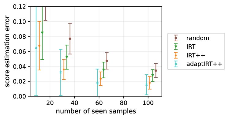
Figure 8: Preliminary adaptive testing results on MMLU.

6.2 Limitations

The main limitations of the methods described in this paper are related to potential severe distribution shifts. Taking MMLU as an example, we anticipate larger performance estimation errors for models that fail on simple questions while answering complicated ones correctly, thus altering the correctness patterns. This might be caused by significant architecture or pre-training data changes. A rapid increase in LLM capabilities may also cause extrapolation errors. To alleviate these problems, we recommend periodically updating the curated examples and IRT parameter estimates using data from more modern LLMs.

7 Acknowledgements

We are grateful for the help provided by Yotam Perlitz in downloading data from HELM.

This paper is based upon work supported by the National Science Foundation (NSF) under grants no. 2027737 and 2113373.

Appendix A Evaluation when subscenarios have different number of samples

Suppose we want to estimate the performance of a scenario $j$ which is composed of $s_{j}$ subscenarios. Denote the set of examples in each subscenario of $j$ as $\mathcal{I}_{jk}$, for $k\in\{1,\cdots,s_{j}\}$. Then, $\mathcal{I}_{j}=\cup_{k}\mathcal{I}_{jk}$, with disjoint $\mathcal{I}_{jk}$’s. For a given LLM $l$, our main goal is then to estimate $\frac{1}{s_{j}}\sum_{k}\frac{1}{|\mathcal{I}_{jk}|}\sum_{i\in\mathcal{I}_{jk}}Y_{il}$. See that we can write

$$\textstyle\frac{1}{s_{j}}\sum_{k}\frac{1}{|\mathcal{I}_{jk}|}\sum_{i\in\mathcal{I}_{jk}}Y_{il}=\sum_{k}\sum_{i\in\mathcal{I}_{jk}}\frac{1}{s_{j}|\mathcal{I}_{jk}|}Y_{il}=\sum_{i\in\mathcal{I}_{j}}\bar{\omega}_{i}Y_{il}.$$

This tells us that we can represent the performance of model $l$ as a weighted average instead of a simple average. In our code, $\omega_{i}\triangleq|\mathcal{I}_{j}|\cdot\bar{\omega}_{i}$’s are called balance_weights and $\bar{\omega}_{i}$’s are called normalized_balance_weights. In Section 3, when computing the estimates using the stratified random sampling strategy, the weights for each example are still given by $1/|\hat{\mathcal{I}}_{j}|$ (because subscenarios should already be equally represented) but when using the clustering ideas, the weight for each anchor point is given by the sum of $\bar{\omega}_{i}$’s of all items in its cluster. We do not apply any weighting when fitting the IRT models but only when computing the p-IRT (and gp-IRT) estimate:

$$\textstyle\hat{Z}^{\text{p-IRT}}_{jl}=\frac{\hat{\lambda}}{|\widehat{\mathcal{I}}_{j}|}\sum_{i\in\widehat{\mathcal{I}}_{j}}\omega_{i}Y_{il}+\frac{1-\hat{\lambda}}{|{\mathcal{I}}_{j}\setminus\widehat{\mathcal{I}}_{j}|}\sum_{i\in{\mathcal{I}}_{j}\setminus\widehat{\mathcal{I}}_{j}}\omega_{i}\hat{p}_{il}.$$

Appendix B tinyMMLU

To construct tinyMMLU we chose 100 examples and weights identified by the IRT anchor point approach (“IRT”) corresponding to the best test performance (across random seeds) in the experiment presented in the top part of Figure 3 on MMLU. For comparison, we analogously selected 100 examples with the correctness anchor point method.

To better understand the composition of tinyMMLU, in Figure 9 we visualize the distribution of the weights of the selected examples and compare it to the weights of the correctness anchors. Recall that weights are non-negative and sum to 1. If an item has a weight $0.1$, for example, that item has a contribution of $10\%$ in the final estimated score. From Figure 9, we can see that tinyMMLU has more uniform weights compared to its correctness-based counterpart. We measure uniformity through the effective sample size (ESS) of the example weights. ESS, traditionally used in the Monte Carlo and domain adaptation (Elvira et al., 2022; Maia Polo & Vicente, 2023) literature, measures weight inequality in a way such that $\text{ESS}=0.50$, for example, informally means that the corresponding weighted average is influenced by only $50\%$ of (uniformly weighted) examples. In the context of our problem, more uniform weights of tinyMMLU contribute to its robustness when evaluating LLMs with varying correctness patterns, such as specialized LLMs in Figure 5.

We also investigate the total weight of the tinyMMLU examples within each of the 57 subjects in Figure 10. The highest weighted are “high school psychology”, “elementary mathematics”, and “professional law”. Interestingly the weight of the subjects is fairly different from its correctness-based counterpart.

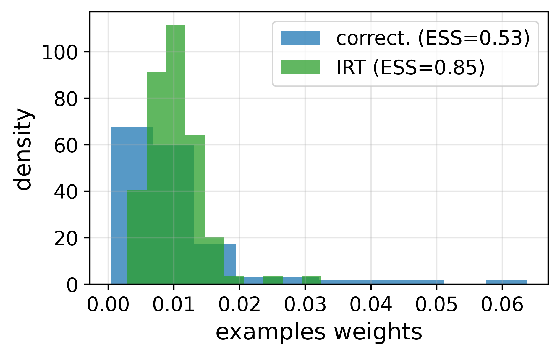
Figure 9: Comparing the spread of examples weights using both the IRT and correctness approaches to find anchor points. We see that weights inequality is much higher when we cluster examples using correctness.

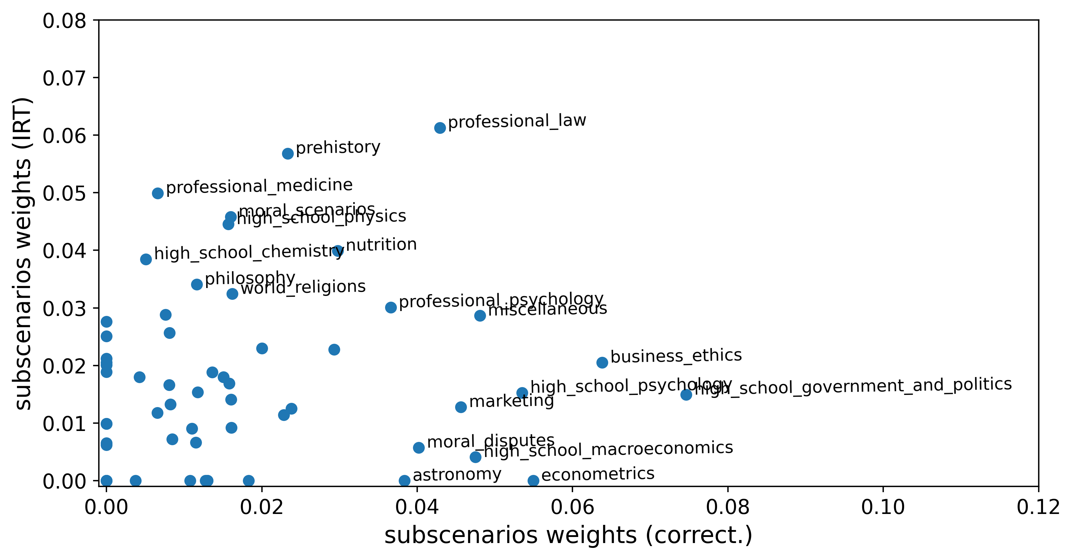
Figure 10: Weights given to MMLU subscenarios by the two anchoring methods.

Appendix C More details about benchmarks

• HuggingFace’s Open LLM Leaderboard (Beeching et al., 2023): the data from this benchmark is composed of 395 LLMs and approx. 29k items that were downloaded from the platform in January/2024. To extract data from those models, we filter all models from the platform that have an MMLU score over $.3$, order them according to their average performance, and equally spaced selected models. Then, we kept all models that had scores for all six scenarios: ARC (Clark et al., 2018), HellaSwag (Zellers et al., 2019), MMLU (Hendrycks et al., 2020), TruthfulQA (Lin et al., 2021), Winogrande (Sakaguchi et al., 2021), and GSM8K (Cobbe et al., 2021). In a second round of data collection, we collected data for 40 “specialized models” by recognizing which models were fine-tuned to do the math, coding, etc.. The two sets of models have an intersection, and in total, we have collected data from 428 LLMs.

• HELM (Liang et al., 2022): we use HELM Lite (https://crfm.stanford.edu/helm/lite) v1.0.0, which is a dataset composed of 37 LLMs and approx. 10k evaluation examples from 10 scenarios. The scenarios are OpenbookQA (Mihaylov et al., 2018), MMLU (Hendrycks et al., 2020), NarrativeQA (Kočiskỳ et al., 2018), NaturalQuestions (closed-book) (Kwiatkowski et al., 2019), NaturalQuestions (open-book), Math (Hendrycks et al., 2021), GSM8K (Cobbe et al., 2021), LegalBench (Guha et al., 2024), MedQA (Jin et al., 2021), WMT14 (Bojar et al., 2014).

Appendix D Extra results

D.1 Running time

We record the running time of IRT inference (ability parameter fitting) when running our experiments. In Figure 11 we show that the average running time is fairly negligible.

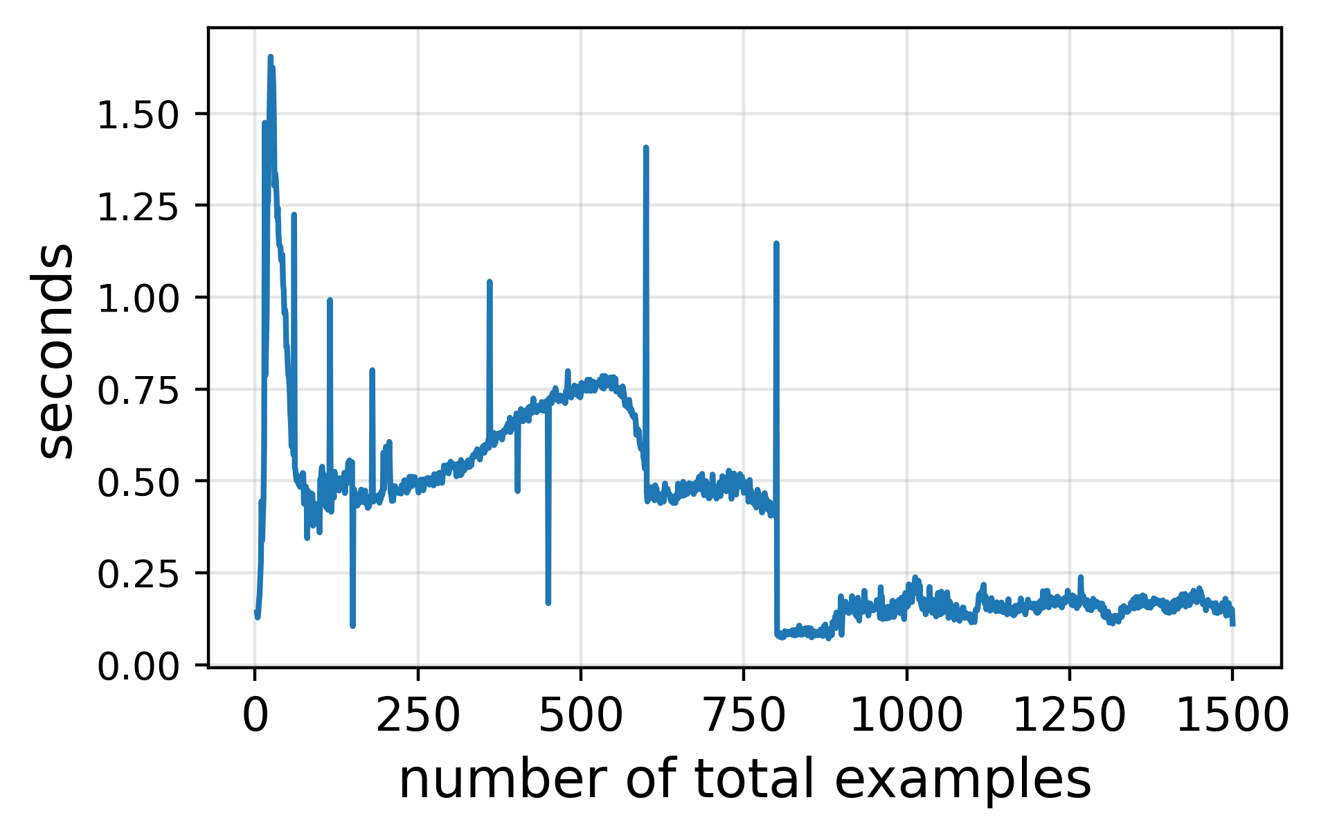
Figure 11: Average running time by the amount of test examples: IRT inference.

D.2 Rank correlation results

In this section, we explore versions of Figures 3 and 5 when we look at rank correlation (correlation between true and predicted ranking) instead of performance. It is clear from the plots below that our method can be used to rank models efficiently with tiny samples.

Figure 12: Rank correlation for true performance and predicted performance among LLMs.

Figure 13: Rank correlation for true performance and predicted performance among LLMs in MMLU. The plot on the left represents a random split of the data while the plot on the right considers specialized models as the test set.

D.3 Adaptive testing

In this section, we complement the results shown in Figure 8 for all benchmarks.

Appendix E Individual performances per scenario

In this section, we explore what is behind Figure 3 by looking in detail at results for individual scenarios for the Open LLM Leaderboard and HELM. It is clear from the following plots that there are scenarios in which our methods shine more than others.

E.1 Open LLM Leaderboard

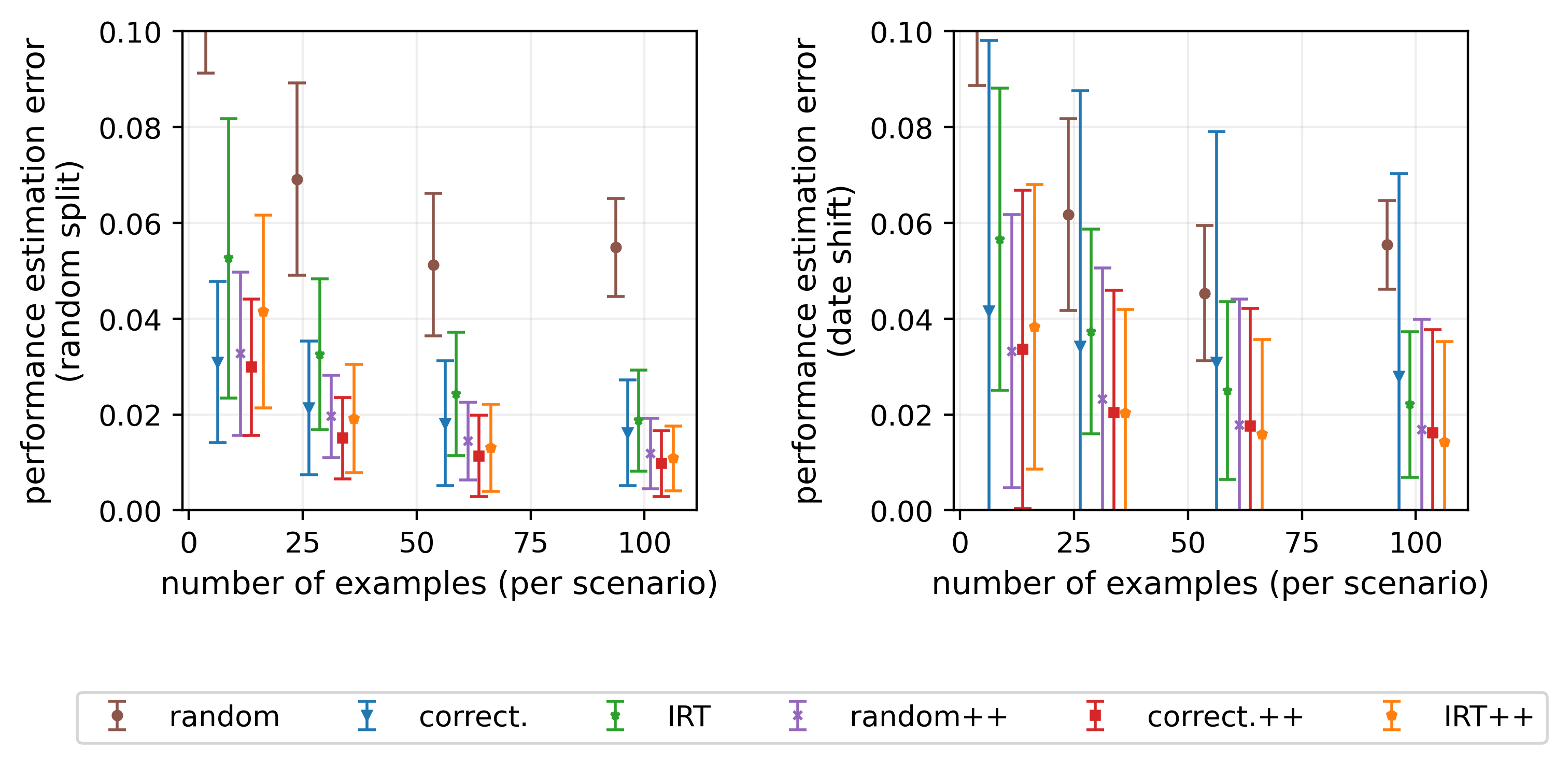
Figure 15: ARC

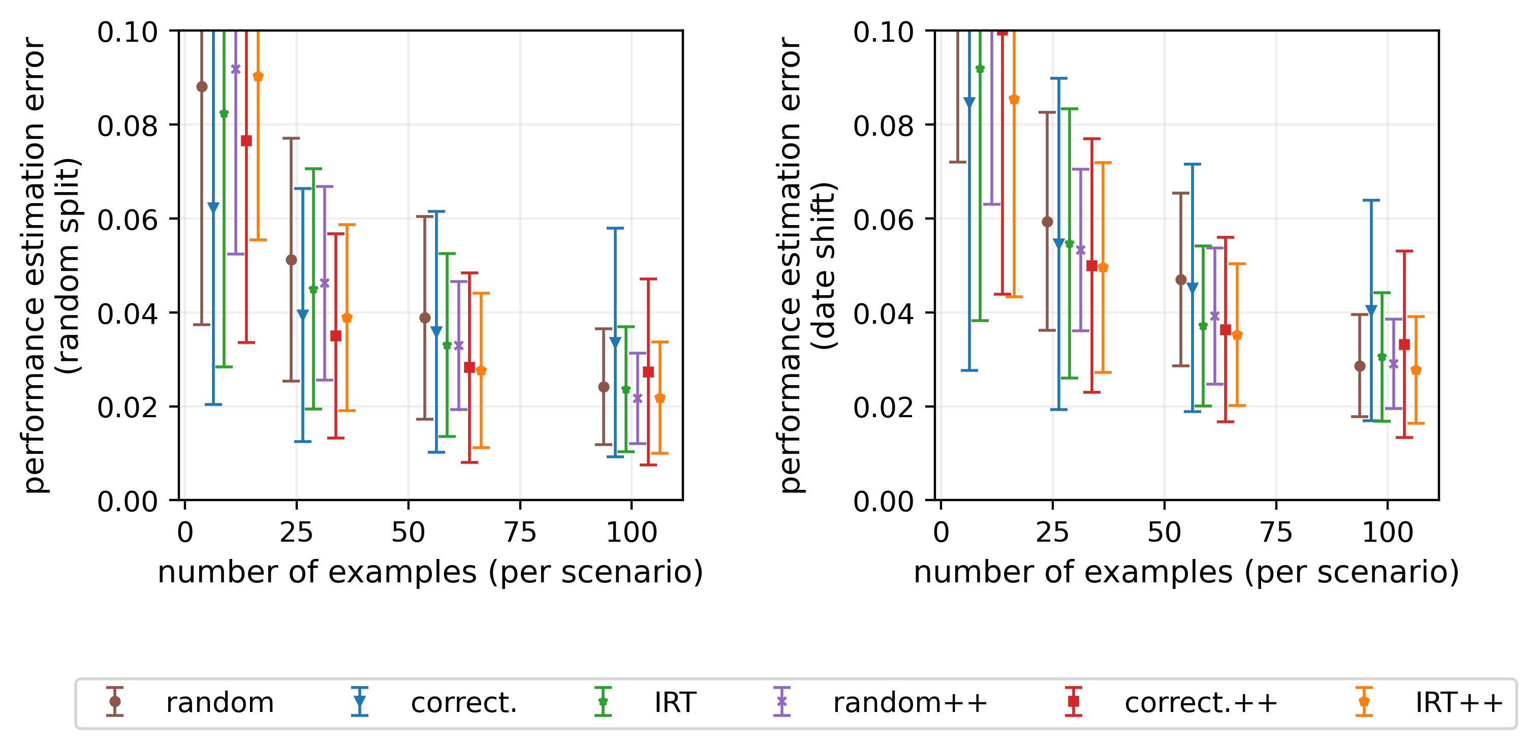
Figure 16: GSM8K

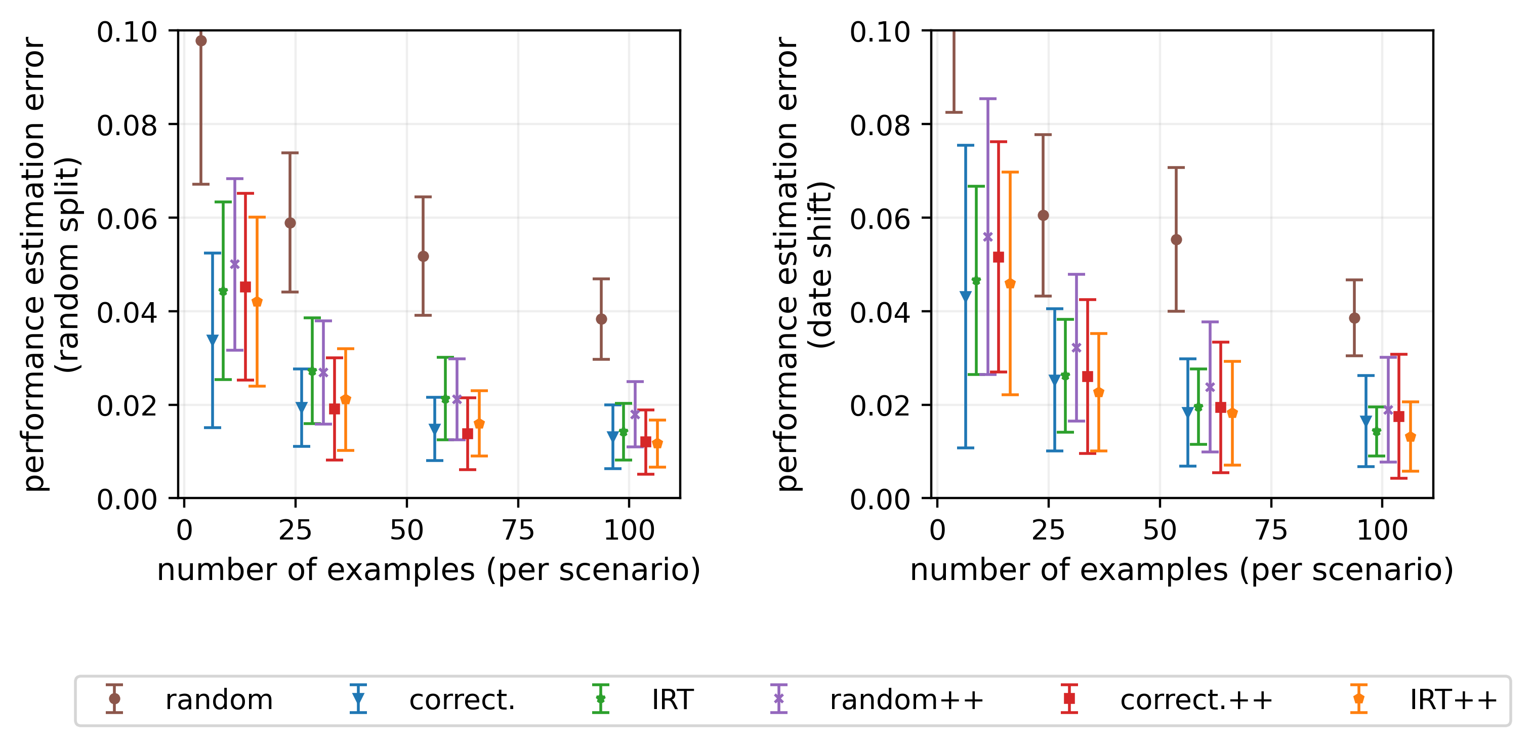
Figure 17: TruthfulQA

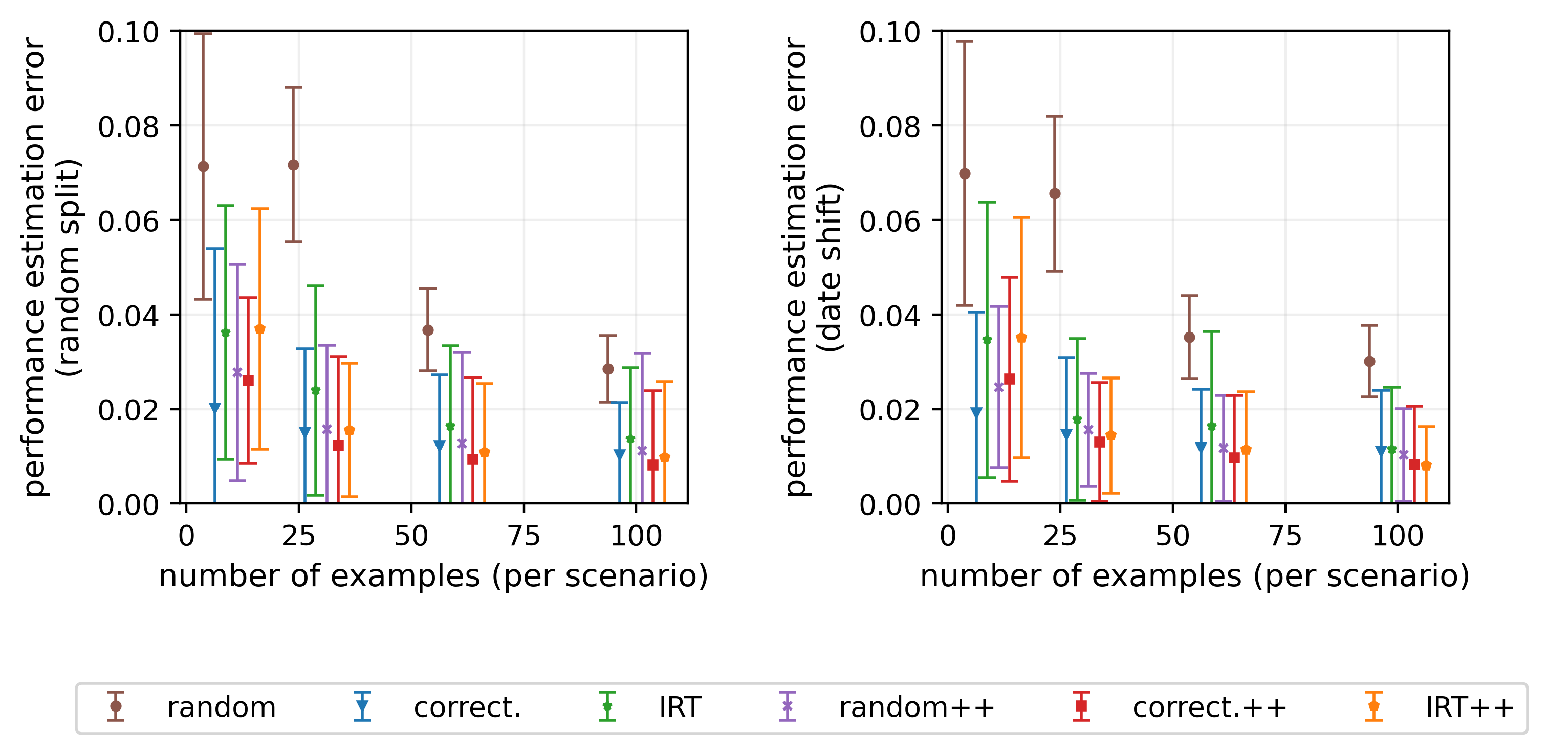
Figure 18: HellaSwag

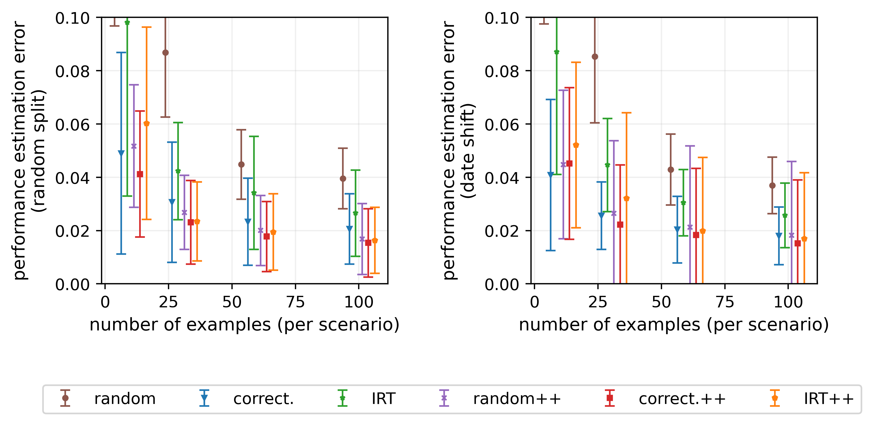
Figure 19: MMLU

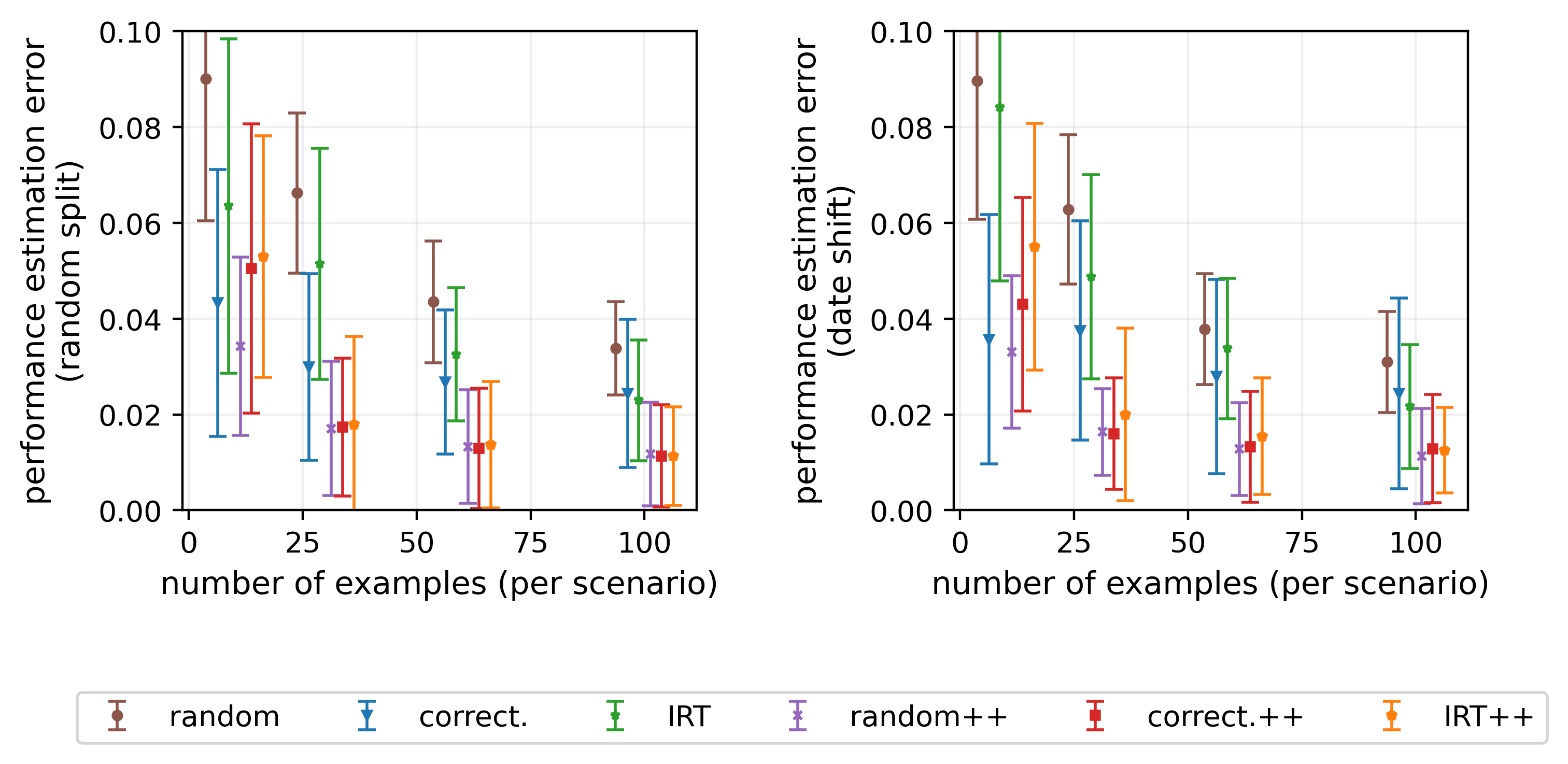
Figure 20: Winogrande

E.2 HELM

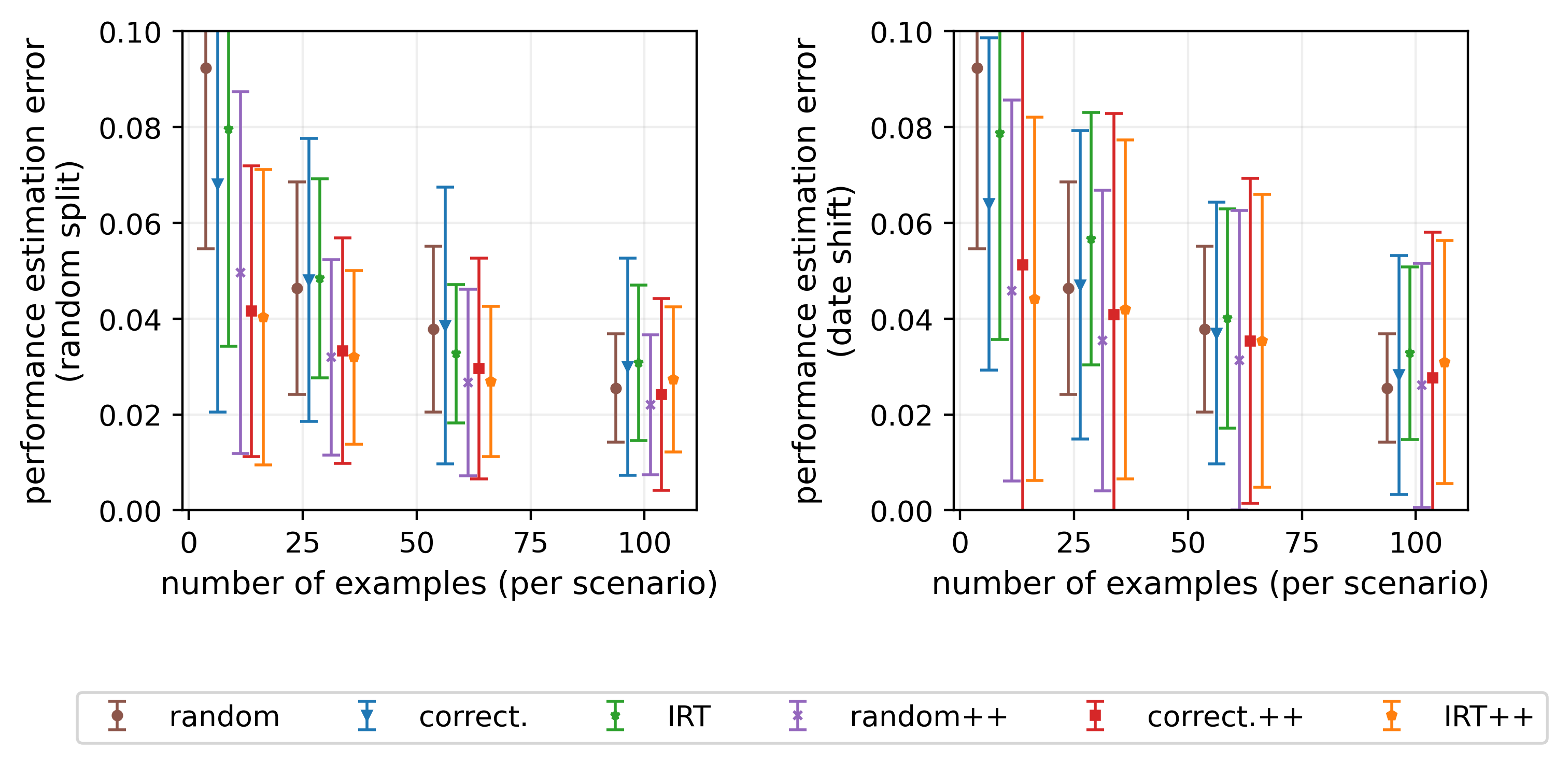
Figure 21: OpenbookQA

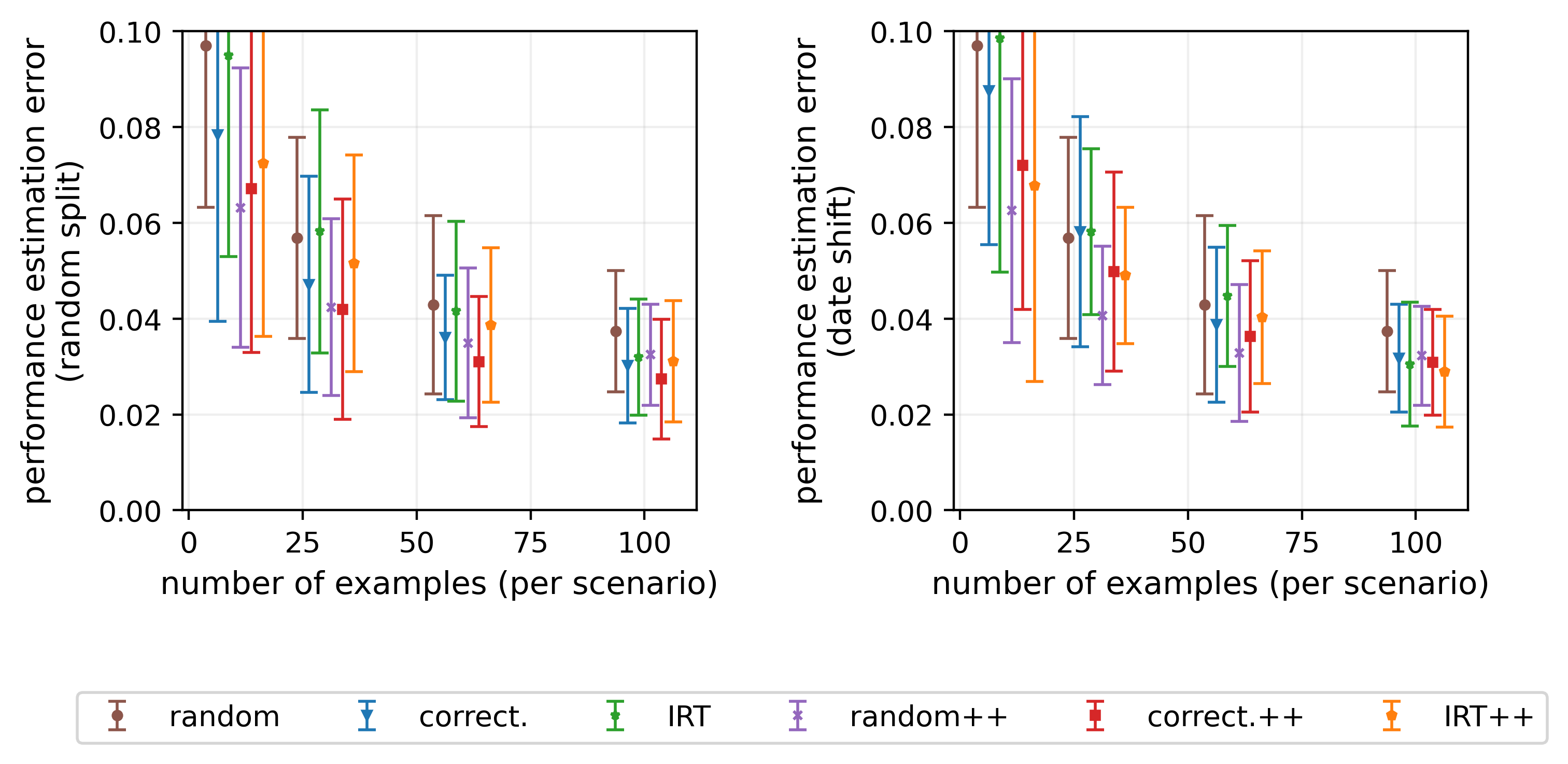
Figure 22: GSM

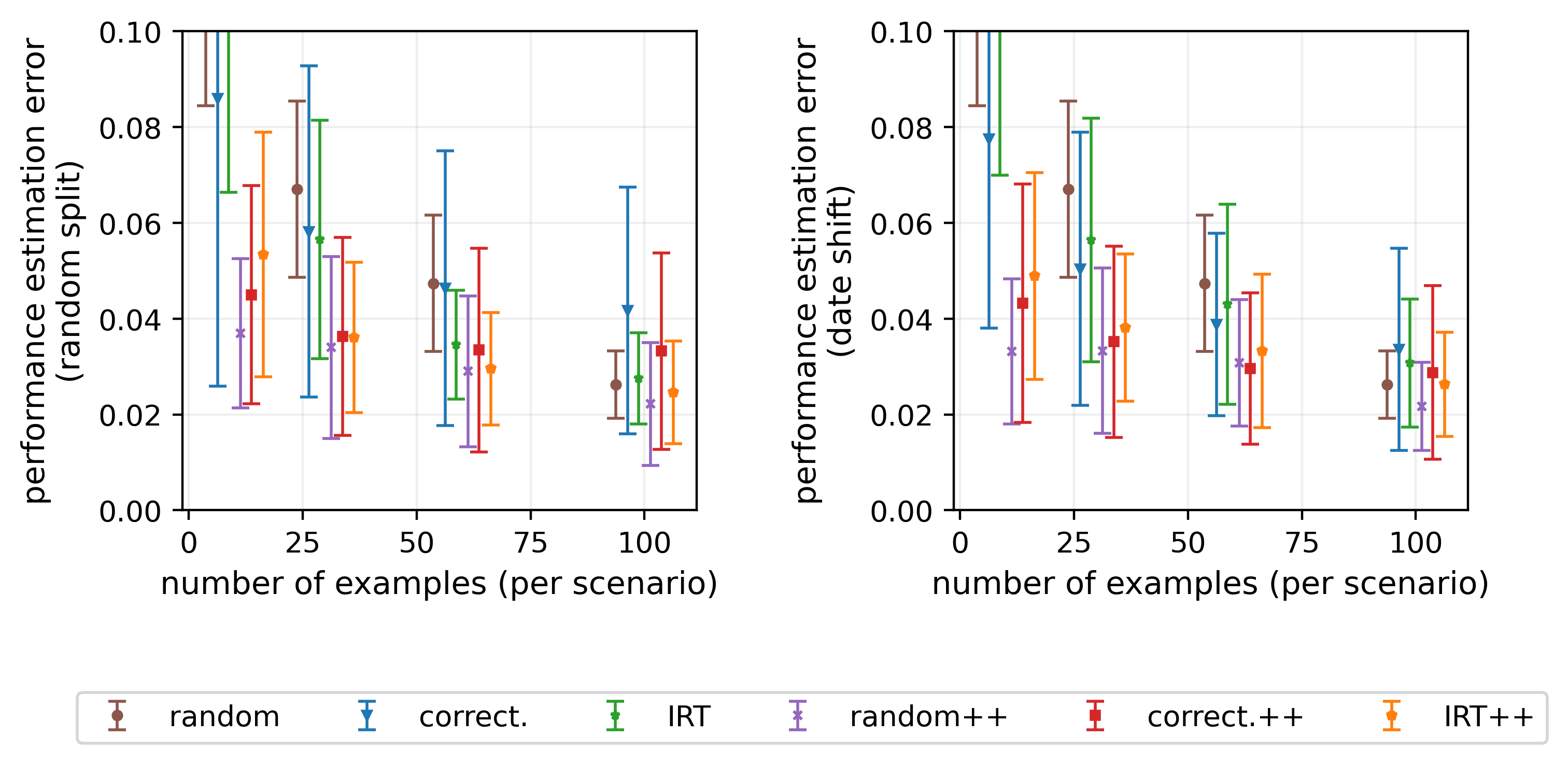
Figure 23: LegalBench

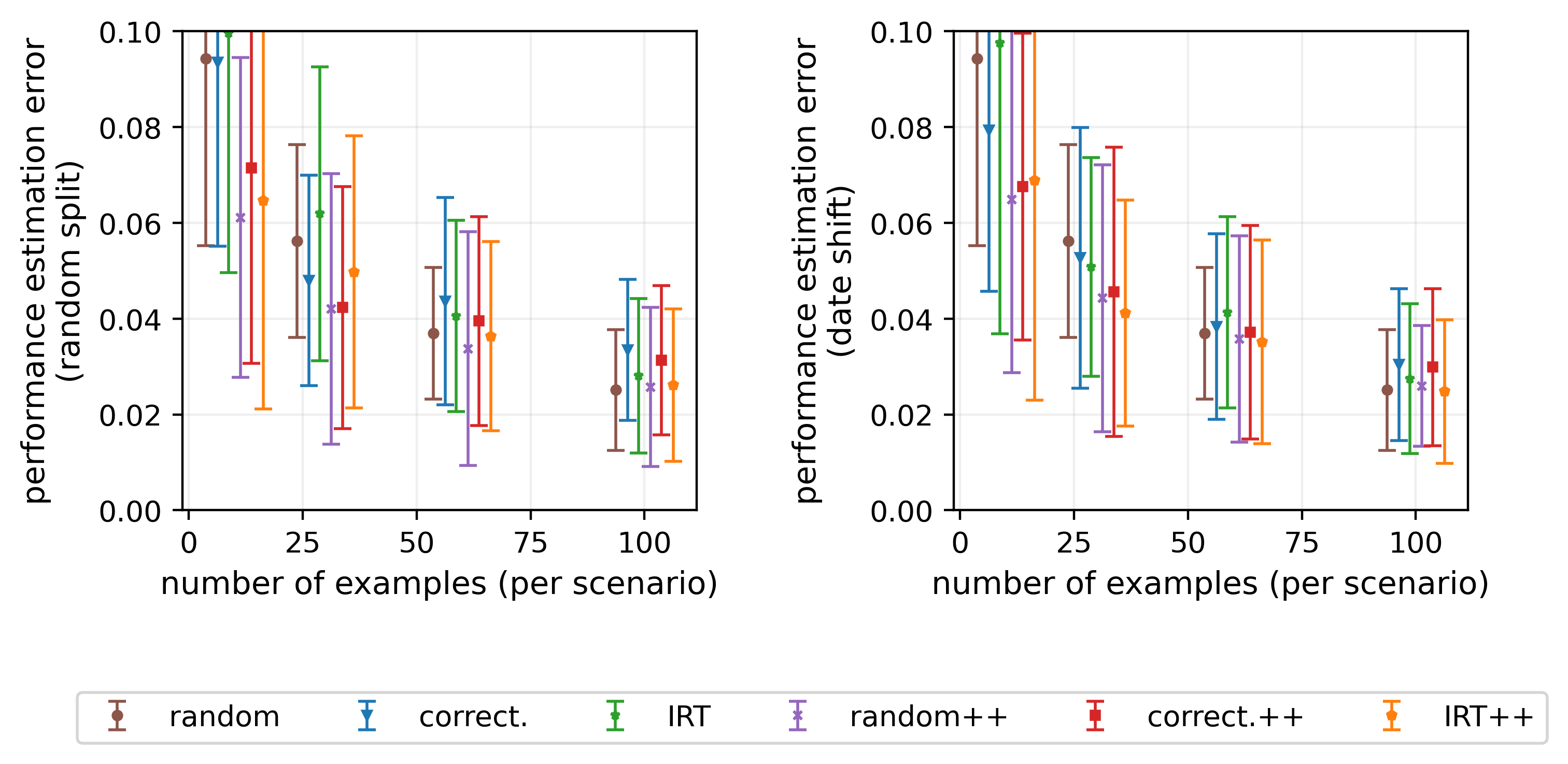
Figure 24: Math

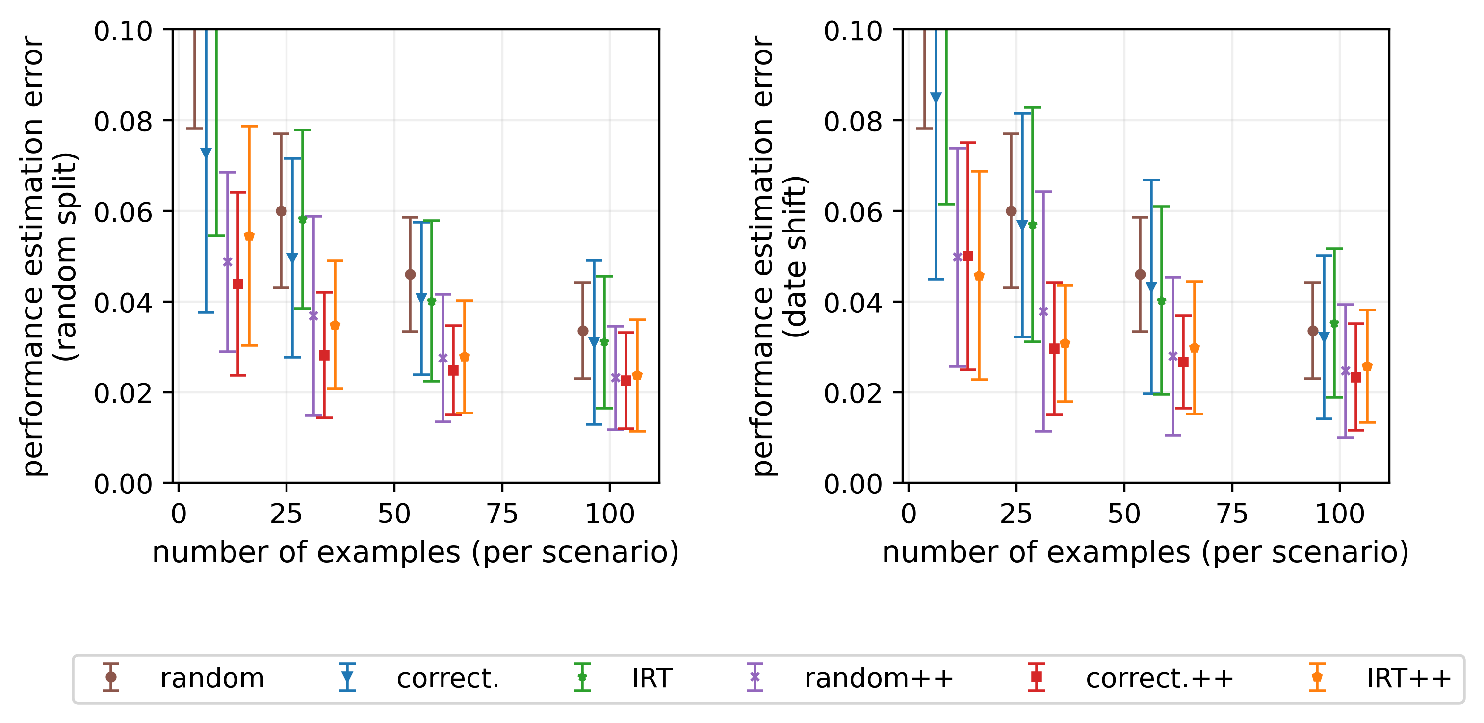
Figure 25: MedQA

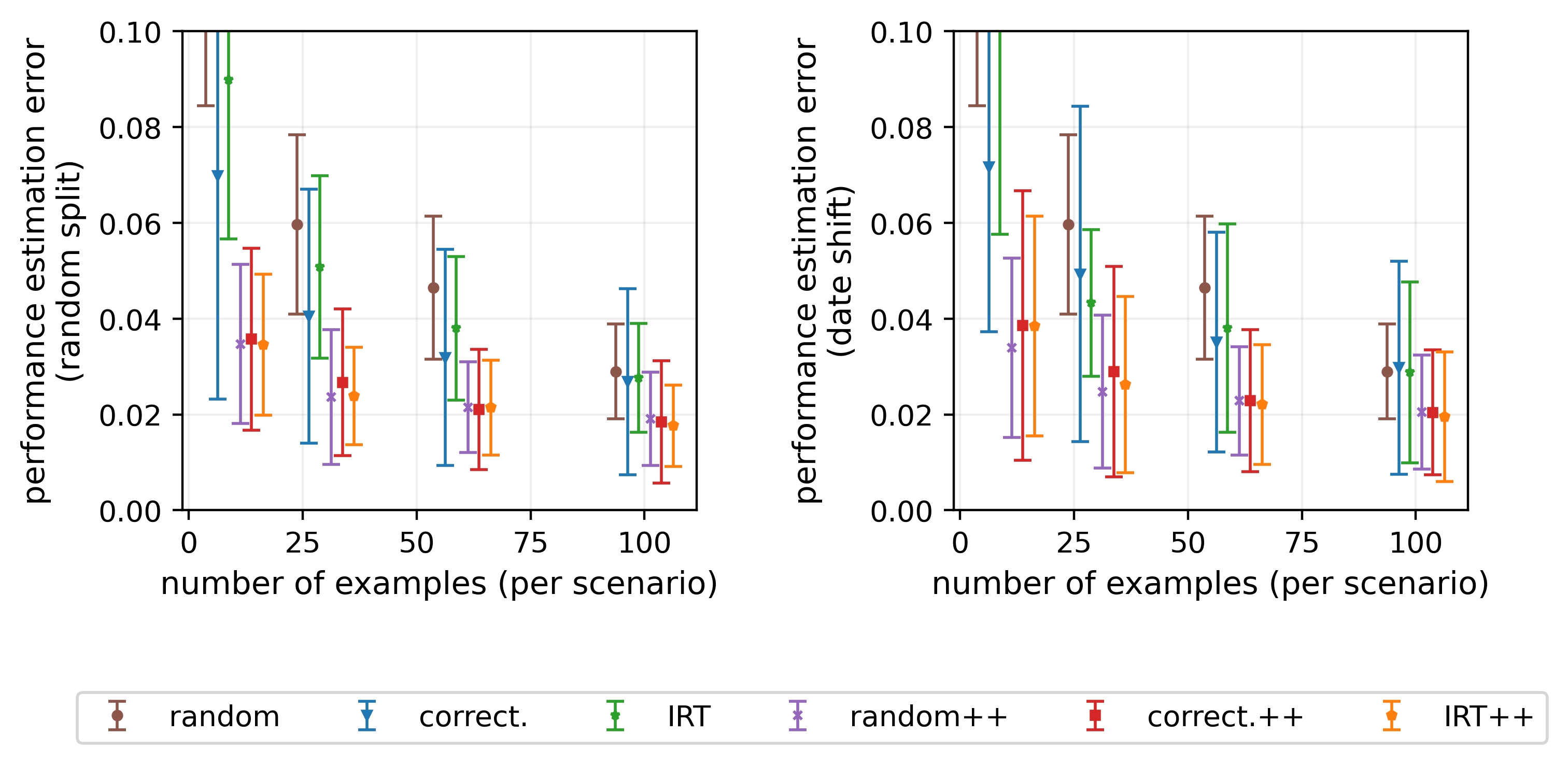
Figure 26: MMLU

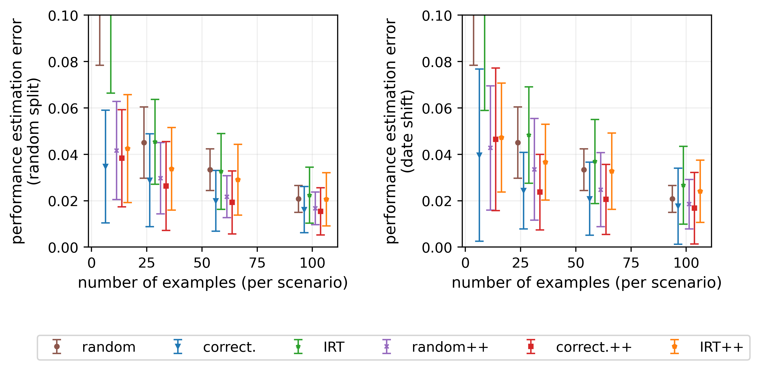
Figure 27: NarrativeQA

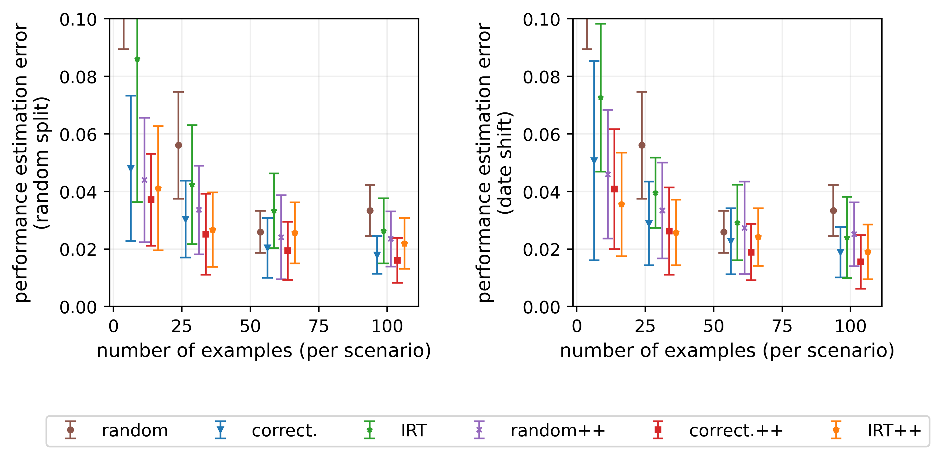
Figure 28: NaturalQA (closed book)

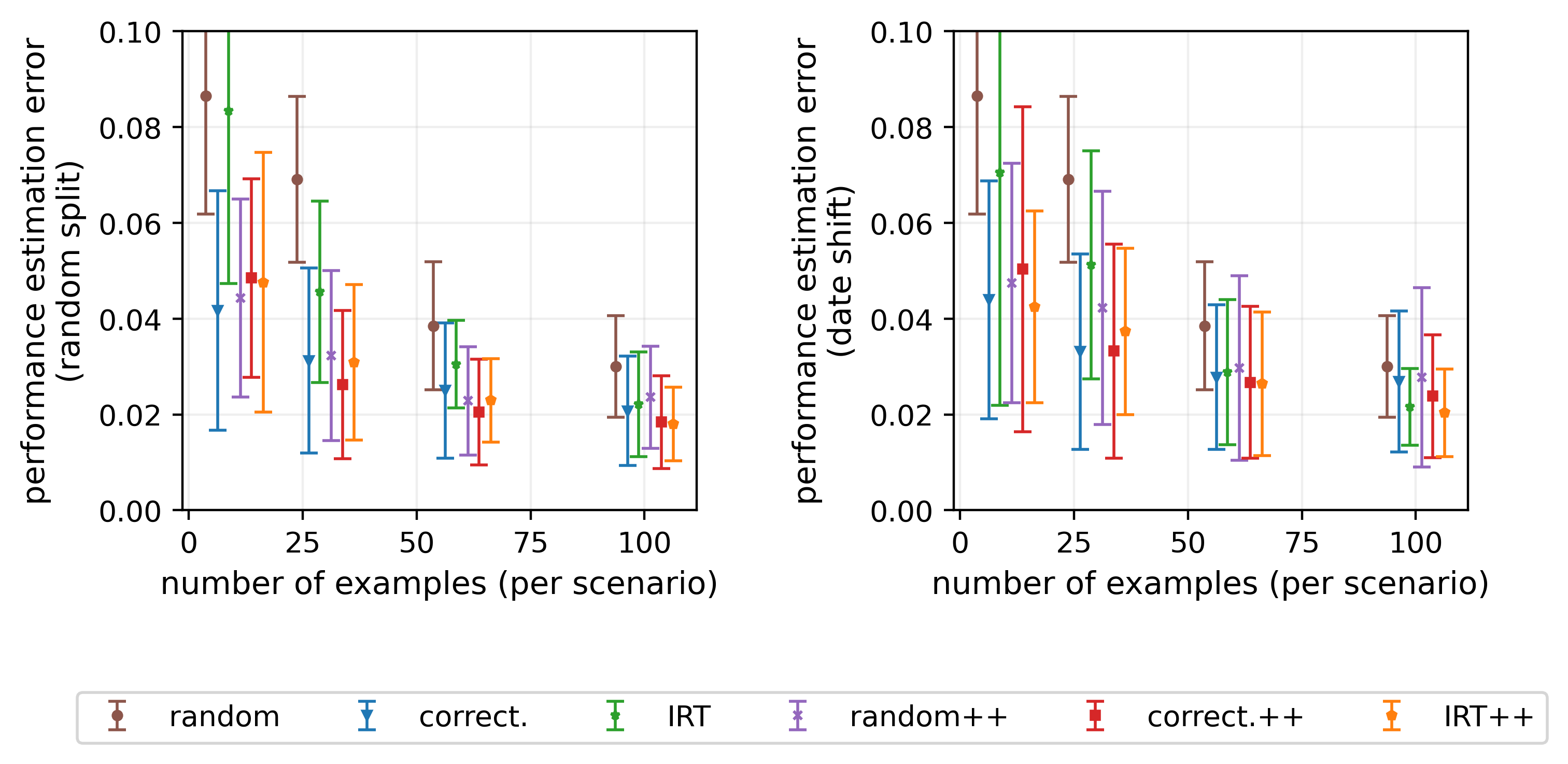
Figure 29: NaturalQA (open book)

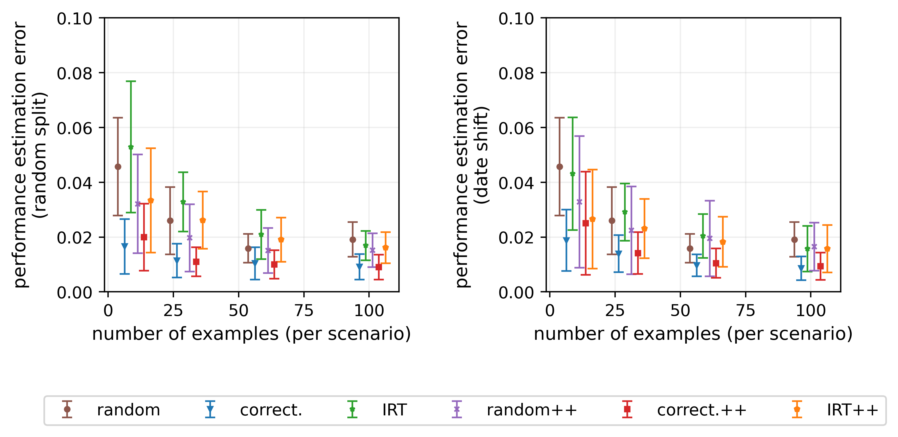
Figure 30: WMT14

References

- Achiam et al. (2023) Achiam, J., Adler, S., Agarwal, S., Ahmad, L., Akkaya, I., Aleman, F. L., Almeida, D., Altenschmidt, J., Altman, S., Anadkat, S., et al. Gpt-4 technical report. arXiv preprint arXiv:2303.08774, 2023.
- An & Yung (2014) An, X. and Yung, Y.-F. Item response theory: What it is and how you can use the irt procedure to apply it. SAS Institute Inc, 10(4):364–2014, 2014.
- Bach et al. (2022) Bach, S., Sanh, V., Yong, Z. X., Webson, A., Raffel, C., Nayak, N. V., Sharma, A., Kim, T., Bari, M. S., Fevry, T., Alyafeai, Z., Dey, M., Santilli, A., Sun, Z., Ben-david, S., Xu, C., Chhablani, G., Wang, H., Fries, J., Al-shaibani, M., Sharma, S., Thakker, U., Almubarak, K., Tang, X., Radev, D., Jiang, M. T.-j., and Rush, A. PromptSource: An integrated development environment and repository for natural language prompts. In Proceedings of the 60th Annual Meeting of the Association for Computational Linguistics: System Demonstrations, pp. 93–104, Dublin, Ireland, 2022. Association for Computational Linguistics. doi: 10.18653/v1/2022.acl-demo.9. URL https://aclanthology.org/2022.acl-demo.9.
- Beeching et al. (2023) Beeching, E., Fourrier, C., Habib, N., Han, S., Lambert, N., Rajani, N., Sanseviero, O., Tunstall, L., and Wolf, T. Open llm leaderboard. https://huggingface.co/spaces/HuggingFaceH4/open_llm_leaderboard, 2023.
- Biderman et al. (2023a) Biderman, S., Prashanth, U. S., Sutawika, L., Schoelkopf, H., Anthony, Q., Purohit, S., and Raf, E. Emergent and predictable memorization in large language models. arXiv preprint arXiv:2304.11158, 2023a.
- Biderman et al. (2023b) Biderman, S., Schoelkopf, H., Anthony, Q. G., Bradley, H., O’Brien, K., Hallahan, E., Khan, M. A., Purohit, S., Prashanth, U. S., Raff, E., Skowron, A., Sutawika, L., and van der Wal, O. Pythia: A suite for analyzing large language models across training and scaling. ArXiv, abs/2304.01373, 2023b. URL https://api.semanticscholar.org/CorpusID:257921893.
- Bojar et al. (2014) Bojar, O., Buck, C., Federmann, C., Haddow, B., Koehn, P., Leveling, J., Monz, C., Pecina, P., Post, M., Saint-Amand, H., et al. Findings of the 2014 workshop on statistical machine translation. In Proceedings of the ninth workshop on statistical machine translation, pp. 12–58, 2014.
- Brown et al. (2020) Brown, T., Mann, B., Ryder, N., Subbiah, M., Kaplan, J. D., Dhariwal, P., Neelakantan, A., Shyam, P., Sastry, G., Askell, A., et al. Language models are few-shot learners. Advances in neural information processing systems, 33:1877–1901, 2020.
- Brzezińska (2020) Brzezińska, J. Item response theory models in the measurement theory. Communications in Statistics-Simulation and Computation, 49(12):3299–3313, 2020.
- Cai et al. (2016) Cai, L., Choi, K., Hansen, M., and Harrell, L. Item response theory. Annual Review of Statistics and Its Application, 3:297–321, 2016.
- Clark et al. (2018) Clark, P., Cowhey, I., Etzioni, O., Khot, T., Sabharwal, A., Schoenick, C., and Tafjord, O. Think you have solved question answering? try arc, the ai2 reasoning challenge. arXiv preprint arXiv:1803.05457, 2018.
- Cobbe et al. (2021) Cobbe, K., Kosaraju, V., Bavarian, M., Chen, M., Jun, H., Kaiser, L., Plappert, M., Tworek, J., Hilton, J., Nakano, R., et al. Training verifiers to solve math word problems. arXiv preprint arXiv:2110.14168, 2021.
- Ein-Dor et al. (2020) Ein-Dor, L., Halfon, A., Gera, A., Shnarch, E., Dankin, L., Choshen, L., Danilevsky, M., Aharonov, R., Katz, Y., and Slonim, N. Active Learning for BERT: An Empirical Study. In Webber, B., Cohn, T., He, Y., and Liu, Y. (eds.), Proceedings of the 2020 Conference on Empirical Methods in Natural Language Processing (EMNLP), pp. 7949–7962, Online, November 2020. Association for Computational Linguistics. doi: 10.18653/v1/2020.emnlp-main.638. URL https://aclanthology.org/2020.emnlp-main.638.
- Elvira et al. (2022) Elvira, V., Martino, L., and Robert, C. P. Rethinking the effective sample size. International Statistical Review, 90(3):525–550, 2022.
- Guha et al. (2024) Guha, N., Nyarko, J., Ho, D., Ré, C., Chilton, A., Chohlas-Wood, A., Peters, A., Waldon, B., Rockmore, D., Zambrano, D., et al. Legalbench: A collaboratively built benchmark for measuring legal reasoning in large language models. Advances in Neural Information Processing Systems, 36, 2024.
- Hastie et al. (2009) Hastie, T., Tibshirani, R., Friedman, J. H., and Friedman, J. H. The elements of statistical learning: data mining, inference, and prediction, volume 2. Springer, 2009.
- Hendrycks et al. (2020) Hendrycks, D., Burns, C., Basart, S., Zou, A., Mazeika, M., Song, D., and Steinhardt, J. Measuring massive multitask language understanding. arXiv preprint arXiv:2009.03300, 2020.
- Hendrycks et al. (2021) Hendrycks, D., Burns, C., Kadavath, S., Arora, A., Basart, S., Tang, E., Song, D., and Steinhardt, J. Measuring mathematical problem solving with the math dataset. arXiv preprint arXiv:2103.03874, 2021.
- Ji et al. (2021) Ji, D., Logan, R. L., Smyth, P., and Steyvers, M. Active bayesian assessment of black-box classifiers. Proceedings of the AAAI Conference on Artificial Intelligence, 35(9):7935–7944, May 2021. doi: 10.1609/aaai.v35i9.16968. URL https://ojs.aaai.org/index.php/AAAI/article/view/16968.
- Jin et al. (2021) Jin, D., Pan, E., Oufattole, N., Weng, W.-H., Fang, H., and Szolovits, P. What disease does this patient have? a large-scale open domain question answering dataset from medical exams. Applied Sciences, 11(14):6421, 2021.
- Katariya et al. (2012) Katariya, N., Iyer, A., and Sarawagi, S. Active evaluation of classifiers on large datasets. In 2012 IEEE 12th International Conference on Data Mining, pp. 329–338, 2012. doi: 10.1109/ICDM.2012.161.
- Kingston & Dorans (1982) Kingston, N. M. and Dorans, N. J. The feasibility of using item response theory as a psychometric model for the gre aptitude test. ETS Research Report Series, 1982(1):i–148, 1982.
- Kočiskỳ et al. (2018) Kočiskỳ, T., Schwarz, J., Blunsom, P., Dyer, C., Hermann, K. M., Melis, G., and Grefenstette, E. The narrativeqa reading comprehension challenge. Transactions of the Association for Computational Linguistics, 6:317–328, 2018.
- Kossen et al. (2021) Kossen, J., Farquhar, S., Gal, Y., and Rainforth, T. Active testing: Sample-efficient model evaluation. In Meila, M. and Zhang, T. (eds.), Proceedings of the 38th International Conference on Machine Learning, volume 139 of Proceedings of Machine Learning Research, pp. 5753–5763. PMLR, 18–24 Jul 2021. URL https://proceedings.mlr.press/v139/kossen21a.html.
- Kwiatkowski et al. (2019) Kwiatkowski, T., Palomaki, J., Redfield, O., Collins, M., Parikh, A., Alberti, C., Epstein, D., Polosukhin, I., Devlin, J., Lee, K., et al. Natural questions: a benchmark for question answering research. Transactions of the Association for Computational Linguistics, 7:453–466, 2019.
- Lalor & Rodriguez (2023) Lalor, J. P. and Rodriguez, P. py-irt: A scalable item response theory library for python. INFORMS Journal on Computing, 35(1):5–13, 2023.
- Lalor et al. (2016) Lalor, J. P., Wu, H., and Yu, H. Building an evaluation scale using item response theory. In Proceedings of the Conference on Empirical Methods in Natural Language Processing. Conference on Empirical Methods in Natural Language Processing, volume 2016, pp. 648. NIH Public Access, 2016.
- Li et al. (2023) Li, X., Zhang, T., Dubois, Y., Taori, R., Gulrajani, I., Guestrin, C., Liang, P., and Hashimoto, T. B. Alpacaeval: An automatic evaluator of instruction-following models. https://github.com/tatsu-lab/alpaca_eval, 2023.
- Liang et al. (2022) Liang, P., Bommasani, R., Lee, T., Tsipras, D., Soylu, D., Yasunaga, M., Zhang, Y., Narayanan, D., Wu, Y., Kumar, A., et al. Holistic evaluation of language models. arXiv preprint arXiv:2211.09110, 2022.
- Lin et al. (2021) Lin, S., Hilton, J., and Evans, O. Truthfulqa: Measuring how models mimic human falsehoods. arXiv preprint arXiv:2109.07958, 2021.
- Liu et al. (2023) Liu, Z., Qiao, A., Neiswanger, W., Wang, H., Tan, B., Tao, T., Li, J., Wang, Y., Sun, S., Pangarkar, O., et al. Llm360: Towards fully transparent open-source llms. arXiv preprint arXiv:2312.06550, 2023.
- Lord et al. (1968) Lord, F., Novick, M., and Birnbaum, A. Statistical theories of mental test scores. 1968.
- Lu et al. (2022) Lu, Y., Bartolo, M., Moore, A., Riedel, S., and Stenetorp, P. Fantastically ordered prompts and where to find them: Overcoming few-shot prompt order sensitivity. In Proceedings of the 60th Annual Meeting of the Association for Computational Linguistics (Volume 1: Long Papers), pp. 8086–8098, Dublin, Ireland, 2022. Association for Computational Linguistics. doi: 10.18653/v1/2022.acl-long.556. URL https://aclanthology.org/2022.acl-long.556.
- Maia Polo & Vicente (2023) Maia Polo, F. and Vicente, R. Effective sample size, dimensionality, and generalization in covariate shift adaptation. Neural Computing and Applications, 35(25):18187–18199, 2023.
- Mihaylov et al. (2018) Mihaylov, T., Clark, P., Khot, T., and Sabharwal, A. Can a suit of armor conduct electricity? a new dataset for open book question answering. arXiv preprint arXiv:1809.02789, 2018.
- Min et al. (2022) Min, S., Lyu, X., Holtzman, A., Artetxe, M., Lewis, M., Hajishirzi, H., and Zettlemoyer, L. Rethinking the role of demonstrations: What makes in-context learning work? In Proceedings of the 2022 Conference on Empirical Methods in Natural Language Processing, pp. 11048–11064, Abu Dhabi, United Arab Emirates, 2022. Association for Computational Linguistics. URL https://aclanthology.org/2022.emnlp-main.759.
- Mishra et al. (2022) Mishra, S., Khashabi, D., Baral, C., Choi, Y., and Hajishirzi, H. Reframing instructional prompts to GPTk’s language. In Findings of the Association for Computational Linguistics: ACL 2022, pp. 589–612, Dublin, Ireland, 2022. Association for Computational Linguistics. doi: 10.18653/v1/2022.findings-acl.50. URL https://aclanthology.org/2022.findings-acl.50.
- Mizrahi et al. (2023) Mizrahi, M., Kaplan, G., Malkin, D., Dror, R., Shahaf, D., and Stanovsky, G. State of what art? a call for multi-prompt llm evaluation. arXiv preprint arXiv:2401.00595, 2023.
- Nie et al. (2020) Nie, Y., Williams, A., Dinan, E., Bansal, M., Weston, J., and Kiela, D. Adversarial nli: A new benchmark for natural language understanding. In Proceedings of the 58th Annual Meeting of the Association for Computational Linguistics, pp. 4885–4901, 2020.
- Perlitz et al. (2023) Perlitz, Y., Bandel, E., Gera, A., Arviv, O., Ein-Dor, L., Shnarch, E., Slonim, N., Shmueli-Scheuer, M., and Choshen, L. Efficient benchmarking (of language models). arXiv preprint arXiv:2308.11696, 2023.
- Petersen et al. (1982) Petersen, N. S. et al. Using item response theory to equate scholastic aptitude test scores. 1982.
- Rodriguez et al. (2021) Rodriguez, P., Barrow, J., Hoyle, A. M., Lalor, J. P., Jia, R., and Boyd-Graber, J. Evaluation examples are not equally informative: How should that change NLP leaderboards? In Zong, C., Xia, F., Li, W., and Navigli, R. (eds.), Proceedings of the 59th Annual Meeting of the Association for Computational Linguistics and the 11th International Joint Conference on Natural Language Processing (Volume 1: Long Papers), pp. 4486–4503, Online, August 2021. Association for Computational Linguistics. doi: 10.18653/v1/2021.acl-long.346. URL https://aclanthology.org/2021.acl-long.346.
- Sakaguchi et al. (2021) Sakaguchi, K., Bras, R. L., Bhagavatula, C., and Choi, Y. Winogrande: An adversarial winograd schema challenge at scale. Communications of the ACM, 64(9):99–106, 2021.
- Sclar et al. (2023) Sclar, M., Choi, Y., Tsvetkov, Y., and Suhr, A. Quantifying language models’ sensitivity to spurious features in prompt design or: How i learned to start worrying about prompt formatting. arXiv preprint arXiv:2310.11324, 2023.
- Song (1988) Song, W. T. Minimal-mse linear combinations of variance estimators of the sample mean. In 1988 Winter Simulation Conference Proceedings, pp. 414–421. IEEE, 1988.
- Srivastava et al. (2022) Srivastava, A., Rastogi, A., Rao, A., Shoeb, A. A. M., Abid, A., Fisch, A., Brown, A. R., Santoro, A., Gupta, A., Garriga-Alonso, A., et al. Beyond the imitation game: Quantifying and extrapolating the capabilities of language models. arXiv preprint arXiv:2206.04615, 2022.
- Taori et al. (2023) Taori, R., Gulrajani, I., Zhang, T., Dubois, Y., Li, X., Guestrin, C., Liang, P., and Hashimoto, T. B. Stanford alpaca: An instruction-following llama model. https://github.com/tatsu-lab/stanford_alpaca, 2023.
- Team et al. (2023) Team, G., Anil, R., Borgeaud, S., Wu, Y., Alayrac, J.-B., Yu, J., Soricut, R., Schalkwyk, J., Dai, A. M., Hauth, A., et al. Gemini: a family of highly capable multimodal models. arXiv preprint arXiv:2312.11805, 2023.
- Touvron et al. (2023) Touvron, H., Martin, L., Stone, K., Albert, P., Almahairi, A., Babaei, Y., Bashlykov, N., Batra, S., Bhargava, P., Bhosale, S., et al. Llama 2: Open foundation and fine-tuned chat models. arXiv preprint arXiv:2307.09288, 2023.
- Van der Linden (2018) Van der Linden, W. J. Handbook of item response theory: Three volume set. CRC Press, 2018.
- Van der Vaart (2000) Van der Vaart, A. W. Asymptotic statistics, volume 3. Cambridge university press, 2000.
- Vania et al. (2021) Vania, C., Htut, P. M., Huang, W., Mungra, D., Pang, R. Y., Phang, J., Liu, H., Cho, K., and Bowman, S. R. Comparing test sets with item response theory. arXiv preprint arXiv:2106.00840, 2021.
- Vivek et al. (2023) Vivek, R., Ethayarajh, K., Yang, D., and Kiela, D. Anchor points: Benchmarking models with much fewer examples. arXiv preprint arXiv:2309.08638, 2023.
- Voronov et al. (2024) Voronov, A., Wolf, L., and Ryabinin, M. Mind your format: Towards consistent evaluation of in-context learning improvements. arXiv preprint arXiv:2401.06766, 2024.
- Wang et al. (2018) Wang, A., Singh, A., Michael, J., Hill, F., Levy, O., and Bowman, S. R. Glue: A multi-task benchmark and analysis platform for natural language understanding. arXiv preprint arXiv:1804.07461, 2018.
- Weber et al. (2023a) Weber, L., Bruni, E., and Hupkes, D. The icl consistency test. arXiv preprint arXiv:2312.04945, 2023a.
- Weber et al. (2023b) Weber, L., Bruni, E., and Hupkes, D. Mind the instructions: a holistic evaluation of consistency and interactions in prompt-based learning. arXiv preprint arXiv:2310.13486, 2023b.
- Wei et al. (2023) Wei, J., Wei, J., Tay, Y., Tran, D., Webson, A., Lu, Y., Chen, X., Liu, H., Huang, D., Zhou, D., et al. Larger language models do in-context learning differently. ArXiv preprint, abs/2303.03846, 2023. URL https://arxiv.org/abs/2303.03846.
- Ye et al. (2023) Ye, Q., Fu, H. Y., Ren, X., and Jia, R. How predictable are large language model capabilities? a case study on big-bench. arXiv preprint arXiv:2305.14947, 2023.
- Yoo et al. (2022) Yoo, K. M., Kim, J., Kim, H. J., Cho, H., Jo, H., Lee, S.-W., Lee, S.-g., and Kim, T. Ground-truth labels matter: A deeper look into input-label demonstrations. In Proceedings of the 2022 Conference on Empirical Methods in Natural Language Processing, pp. 2422–2437, Abu Dhabi, United Arab Emirates, 2022. Association for Computational Linguistics. URL https://aclanthology.org/2022.emnlp-main.155.
- Zellers et al. (2019) Zellers, R., Holtzman, A., Bisk, Y., Farhadi, A., and Choi, Y. Hellaswag: Can a machine really finish your sentence? arXiv preprint arXiv:1905.07830, 2019.