This paper has been accepted for publication in IEEE Robotics and Automation Letters.

This is the author’s version of an article that has, or will be, published in this journal or conference. Changes were, or will be, made to this version by the publisher prior to publication.

DOI:	10.1109/LRA.2024.3367270
IEEE Xplore:	https://ieeexplore.ieee.org/document/10439640

Please cite this paper as:

T. Hitchcox and J. R. Forbes, “Laser-to-Vehicle Extrinsic Calibration in Low-Observability Scenarios for Subsea Mapping,” in IEEE Robotics and Automation Letters, vol. X, no. X, pp. XX-XX, 2024.

©2024  IEEE. Personal use of this material is permitted. Permission from IEEE must be obtained for all other uses, in any current or future media, including reprinting/republishing this material for advertising or promotional purposes, creating new collective works, for resale or redistribution to servers or lists, or reuse of any copyrighted component of this work in other works.

Laser-to-Vehicle Extrinsic Calibration in Low-Observability Scenarios for Subsea Mapping

Abstract

Laser line scanners are increasingly being used in the subsea industry for high-resolution mapping and infrastructure inspection. However, calibrating the 3D pose of the scanner relative to the vehicle is a perennial source of confusion and frustration for industrial surveyors. This work describes three novel algorithms for laser-to-vehicle extrinsic calibration using naturally occurring features. Each algorithm makes a different assumption on the quality of the vehicle trajectory estimate, enabling good calibration results in a wide range of situations. A regularization technique is used to address low-observability scenarios frequently encountered in practice with large, rotationally stable subsea vehicles. Experimental results are provided for two field datasets, including the recently discovered wreck of the Endurance.

I Introduction

Sensor-to-vehicle extrinsics define the 3D pose of a sensor relative to the vehicle. An accurate extrinsic estimate is critical for mapping applications, as data collected from the sensor must be resolved in a common reference frame using the vehicle’s estimated trajectory. Errors in the extrinsic estimate will therefore have a direct impact on map quality.

The subsea industry is increasingly using laser line scanners to produce millimeter-resolution reconstructions of underwater assets. To accurately assess potential damage to these assets, the pose of the laser relative to the vehicle must be known to within tenths of a degree and fractions of a centimeter. However, calibrating the laser-to-vehicle extrinsics is currently a challenge in the subsea industry. Computer-aided design (CAD) models of an underwater vehicle and sensor payload should provide a good initial pose estimate, however as-designed and as-deployed configurations can differ due to in-field modifications. “Patch test” operations are performed to refine an extrinsic estimate, where a vehicle makes multiple passes over the same patch of seabed, typically following prescribed maneuvers to isolate the effects of individual degrees of freedom. Patch tests are long and tedious, with extrinsic refinement often performed manually to achieved a visually pleasing map. This paper delivers a straightforward, optimization-based approach to address this problem.

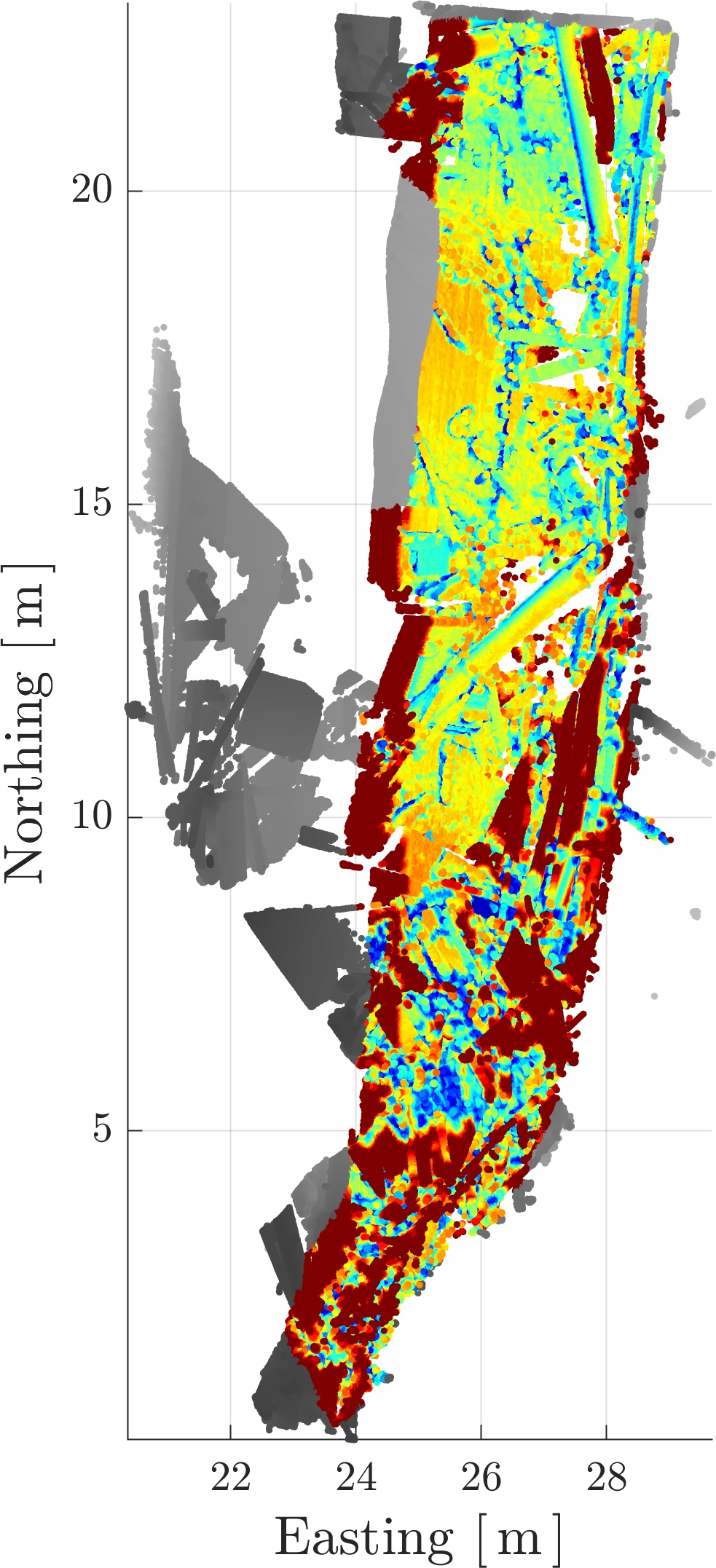
(a) Prior

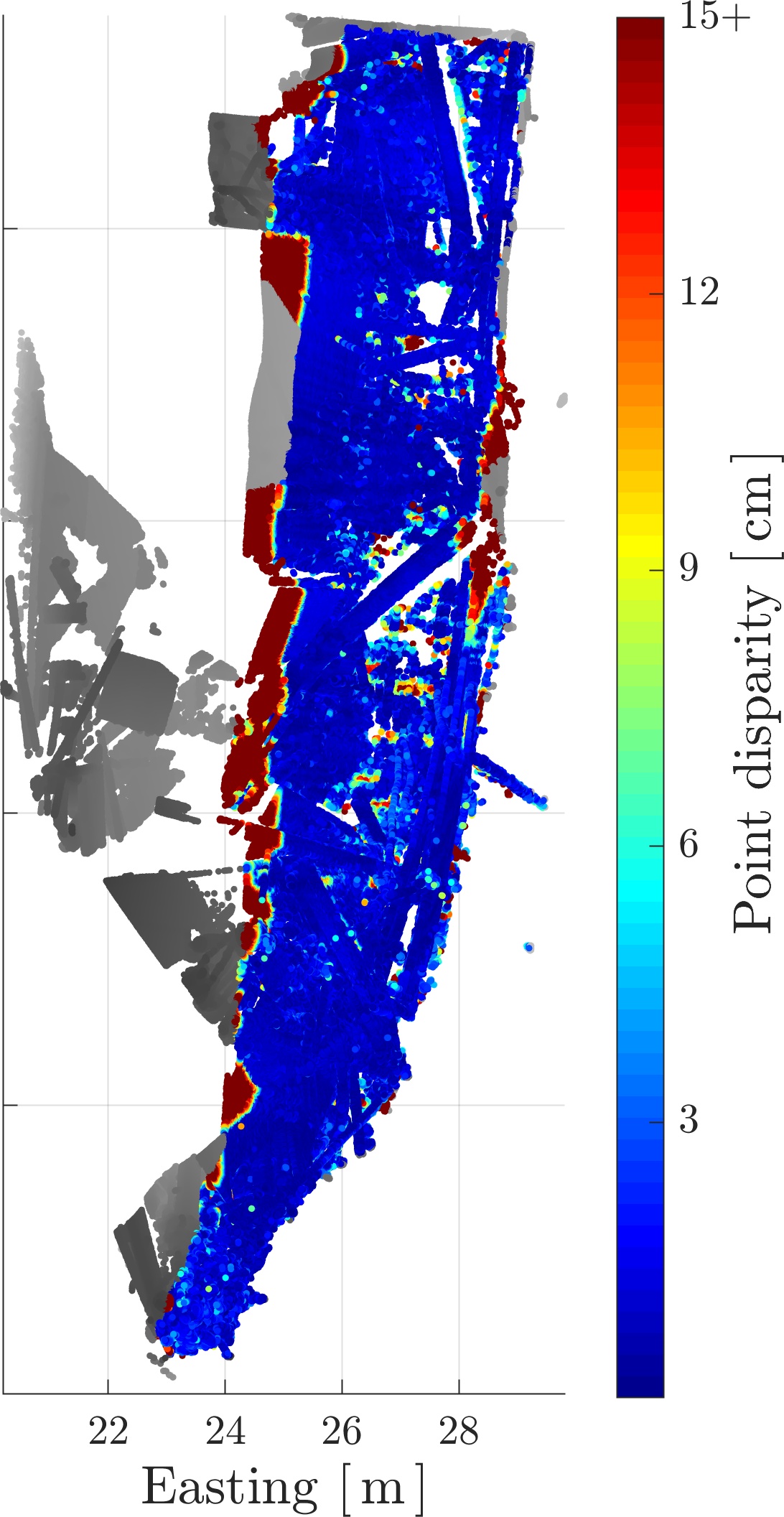
(b) Posterior, Algorithm 2

Figure 1: Patch test scans of the Endurance shipwreck, with point disparity errors [1] shown before and after joint extrinsic and trajectory optimization. Included with permission from the Falklands Maritime Heritage Trust.

Sensor-to-vehicle extrinsic calibration has been extensively studied in the literature. A general theory for spatial and temporal calibration is given in [2], which uses a continuous-time trajectory representation based on B-splines. A second general calibration framework presented in [3] uses a maximum-likelihood approach, with refinement through the minimization of various appearance-based metrics.

Few studies consider laser profile scanners, however [4] provides a solution for laser-to-camera calibration. Studies investigating lidar-to-IMU calibration are much more common. For example, [5] provides a method for calibrating lidar-to-INS extrinsics by maximizing an entropy metric, which represents the compactness of the resulting point cloud. Online lidar-to-IMU calibration is performed in [6] as part of a lidar-inertial sliding window odometry framework. A continuous-time B-spline trajectory representation is used for targetless lidar-to-IMU calibration in [7].

During sensor extrinsic calibration, certain degenerate motion patterns result in poor observability of calibration parameters. These patterns are identified in [8, 3, 9], with the need for roll and pitch excitation for extrinsic calibration on ground vehicles identified in [5]. An observability-aware approach for extrinsic calibration is developed in [10], which uses singular value decomposition to identify good sections of calibration data and to modify the state update during optimization. The same observability-aware approach to data selection is used in [11], which bounds the magnitude of the state update assuming that a good initial estimate is available.

This work develops three novel algorithms for calibrating the pose of a laser line scanner to a vehicle’s inertial navigation system (INS). The algorithms calibrate all six degrees of freedom simultaneously by optimizing over the matrix Lie group $SE(3)$, eliminating the need for complicated patch test maneuvers and manual tuning. Calibration is performed using naturally-occurring 3D features without the need for a reference target, and has been adapted for use with rotationally stable underwater vehicles. The algorithms are validated on two challenging underwater field datasets, including a 3D laser reconstruction of the historic Endurance shipwreck (Figure 1).

II Preliminaries

II-A Reference Frames and Navigation Conventions

This section discusses the reference frames and navigation conventions used in this paper. A three-dimensional dextral reference frame ${\mathcal{F}_{a}}$ is composed of three orthonormal basis vectors. The position of point $z$ relative to point $w$ is resolved in ${\mathcal{F}_{a}}$ as ${\mbf{r}^{zw}_{a}\in\mathbb{R}^{3}}$ and in frame ${\mathcal{F}_{b}}$ as $\mbf{r}^{zw}_{b}$. These quantities are related via ${\mbf{r}^{zw}_{a}=\mbf{C}_{ab}\mbf{r}^{zw}_{b}}$, with $\mbf{C}_{ab}$ a direction cosine matrix, ${\mbf{C}\in SO(3)=\{\mbf{C}\in\mathbb{R}^{3\times 3}\,|\,\mbf{C}\mbf{C}^{\mathsf{T}}=\mbf{1},\det\mbf{C}=+1\}}$ [12, §7.1.1]. Time-varying quantities are indicated by the subscript $(\cdot)_{k}$, for example $\mbf{r}^{z_{k}w}_{a}$ describes the position of moving point $z$ at time $t_{k}$. In this work ${\mathcal{F}_{a}}$ is the local geodetic navigation frame, ${\mathcal{F}_{b}}$ is the vehicle frame, and ${\mathcal{F}_{\ell}}$ is the reference frame of the laser. Following maritime convention, ${\mathcal{F}_{a}}$ and ${\mathcal{F}_{b}}$ are north-east-down (NED) reference frames, while the east-north-up (ENU) reference frame of the laser is shown in Figure 2. Finally, point $w$ is the world datum, point $z$ is the vehicle datum, and point $s$ is the laser datum.

II-B Matrix Lie Groups

The 3D pose of a vehicle at time $t_{k}$ is represented as an element of the matrix Lie group $SE(3)$,

$$\mbf{T}^{z_{k}w}_{ab_{k}}=\begin{bmatrix}\mbf{C}_{ab_{k}}&\mbf{r}^{z_{k}w}_{a}\\ \mbf{0}&1\end{bmatrix}\in SE(3),$$ (1)

with ${SE(3)=\{\mbf{T}\in\mathbb{R}^{4\times 4}\,|\,\mbf{C}\in SO(3),\mbf{r}\in\mathbb{R}^{3}\}}$ [12, §7.1.1]. In estimation problems involving matrix Lie groups, perturbations and uncertainty are modeled in the matrix Lie algebra ${\mathfrak{se}(3)\triangleq T{1}SE(3)}$ [13], with ${\bm{\xi}^{\wedge}\in\mathfrak{se}(3)}$. The “wedge” operator is ${(\cdot)^{\wedge}:\mathbb{R}^{6}\to\mathfrak{se}(3)}$, while the “vee” operator is ${(\cdot)^{\vee}:\mathfrak{se}(3)\to\mathbb{R}^{6}}$, such that ${(\bm{\xi}^{\wedge})^{\vee}=\bm{\xi}}$. A Lie group and Lie algebra are related by the exponential map, which for matrix Lie groups is the matrix exponential,

$$\mbf{T}=\exp(\bm{\xi}^{\wedge}).\vspace{-3pt}$$ (2)

The matrix logarithm is used to return to the Lie algebra via

$$\bm{\xi}^{\wedge}=\log(\mbf{T}).\vspace{-3pt}$$ (3)

Errors on matrix Lie groups are defined multiplicatively. This work uses a left-invariant error definition [14, §2.3],

$$\delta\mbf{T}=\mbf{T}^{-1}\tilde{\mbf{T}},\vspace{-3pt}$$ (4)

where $\mbf{T}$ is the current state estimate and $\tilde{\mbf{T}}$ is a state estimate generated from a predictive model or prior information. The corresponding perturbation scheme is

$$\mbf{T}=\bar{\mbf{T}}\exp(-\delta\bm{\xi}^{\wedge}),$$ (5)

with perturbation ${\delta\bm{\xi}\sim\mathcal{N}(\mbf{0},\bm{\Sigma})}$, ${\bm{\Sigma}=\mathrm{E}[\,\delta\bm{\xi}\,\delta\bm{\xi}^{\mathsf{T}}]\in\mathbb{R}^{6\times 6}}$. The state estimate is therefore defined by mean estimate $\bar{\mbf{T}}$ and covariance $\bm{\Sigma}$. Finally, this work makes use of the $(\cdot)^{\odot}$ operator, ${(\cdot)^{\odot}:\mathbb{R}^{4}\to\mathbb{R}^{4\times 6}}$ [12, §7.1.8], defined here for homogeneous point ${\mbf{u}=[\,\mbf{r}^{\mathsf{T}}\ 1]^{\mathsf{T}}}$, ${\mbf{r}\in\mathbb{R}^{3}}$ as

$$\mbf{u}^{\odot}=\begin{bmatrix}-\mbf{r}^{\times}&\mbf{1}\\ \mbf{0}&\mbf{0}\end{bmatrix},$$ (6)

with $(\cdot)^{\times}$ the skew-symmetric operator [12, §7.1.2].

II-C Batch State Estimation

Given a set of states ${\bm{\mathcal{X}}=\{\mbf{x}_{i}\}^{N}_{i=1}}$ to be estimated, a set of measurements ${\bm{\mathcal{Y}}=\{\mbf{y}_{j}\}^{M}_{j=1}}$ relating to the states, and prior estimates ${\bm{\mathcal{Z}}=\{\mbf{z}_{i}\}^{N}_{i=1}}$ of the states, batch state estimation seeks to produce a maximum a posteriori (MAP) solution,

$$\bm{\mathcal{X}}_{\star}=\operatorname*{arg\,max}_{\bm{\mathcal{X}}}\,p\left(\bm{\mathcal{X}}\,|\,\bm{\mathcal{Y}},\bm{\mathcal{Z}}\right).\vspace{-3pt}$$ (7)

Invoking Bayes’ rule, assuming Gaussian measurement noise densities, and taking the negative log likelihood transforms (7) into a new optimization problem [12, §3.1.2],

$$\bm{\mathcal{X}}_{\star}=\operatorname*{arg\,min}_{\bm{\mathcal{X}}}\,J(\bm{\mathcal{X}}),\vspace{-3pt}$$ (8)

in which the least-squares objective function $J(\bm{\mathcal{X}})$ is

$$J(\bm{\mathcal{X}})=\frac{1}{2}\sum^{N}_{i=1}\|\mbf{e}_{i}\!\left(\mbf{z}_{i},\mbf{x}_{i}\right)\!\|^{2}_{\mbf{P}_{i}^{-1}}+\frac{1}{2}\sum^{M}_{j=1}\|\mbf{e}_{j}\!\left(\mbf{y}_{j},\bm{\mathcal{X}}_{j}\right)\!\|^{2}_{\mbf{M}_{j}^{-1}}.\vspace{-3pt}$$ (9)

Here, $\mbf{e}_{i}$ denotes the prior errors, $\mbf{e}_{j}$ denotes the measurement errors, $\bm{\mathcal{X}}_{j}$ is the set of states involved in defining error $\mbf{e}_{j}$, and $\|\mbf{e}\|^{2}_{\bm{\Sigma}^{-1}}$ is the squared Mahalanobis distance,

$$\|\mbf{e}\|^{2}_{\bm{\Sigma}^{-1}}\triangleq\mbf{e}^{\mathsf{T}}\bm{\Sigma}^{-1}\mbf{e}\in\mathbb{R}_{\geq 0},$$ (10)

with $\mbf{P}_{i}$, $\mbf{M}_{j}$ denoting the covariance on the prior and measurement errors, respectively. Equation 8 is solved by repeatedly linearizing objective function (9) about the current operating point $\bar{\bm{\mathcal{X}}}$ and obtaining the local minimizing increment $\delta\bm{\mathcal{X}}_{\star}$ using, for example, Gauss-Newton or Levenberg-Marquardt [12, §4.3.1]. For a problem on matrix Lie groups, the Gauss-Newton update is

$$\delta\bm{\xi}_{\star}=-\big{(}\mbf{F}^{\mathsf{T}}\mbf{W}\,\mbf{F}\big{)}^{-1}\mbf{F}^{\mathsf{T}}\mbf{W}\,\mbf{e},$$ (11)

in which ${\delta\bm{\xi}_{\star}=[\,\delta\bm{\xi}_{1}^{\mathsf{T}}\ \ldots\ \delta\bm{\xi}_{N}^{\mathsf{T}}\,]^{\mathsf{T}}}$, $\mbf{e}$ contains the stacked $\mbf{e}_{i}$ and $\mbf{e}_{j}$, $\mbf{W}$ is a sparse matrix with the $\mbf{P}_{i}^{-1}$ and $\mbf{M}_{j}^{-1}$ on the main block diagonal, and Jacobian $\mbf{F}$ contains the individual ${\mbf{F}_{i}=\frac{\partial\mbf{e}_{i}}{\partial\bm{\xi}_{i}}\big{|}_{\bar{\mbf{T}}_{i}}\!}$ and ${\mbf{F}^{i}_{j}=\frac{\partial\mbf{e}_{j}}{\partial\bm{\xi}_{i}}\big{|}_{\bar{\mbf{T}}_{i}}\!}$ arranged accordingly. With a left-invariant error definition (4), the $SE(3)$ states are updated as

$$\mbf{T}_{i}\leftarrow\mbf{T}_{i}\exp\left(-\delta\bm{\xi}_{i}^{\wedge}\right).$$ (12)

TABLE I: Three algorithms for laser-to-INS extrinsic calibration

Alg.	Assumptions	Design variables	Figure	Section
1	Perfect DVL-INS navigation estimate	Laser-to-INS extrinsics	Figure 3	III-D1
2	Good local navigation, global submap drift	Laser-to-INS extrinsics, global submap poses	Figure 4	III-D2
3	Poor DVL-INS navigation estimate	Laser-to-INS extrinsics, submap shape	Figure 5	III-D3

II-D Subsea Laser Scanning

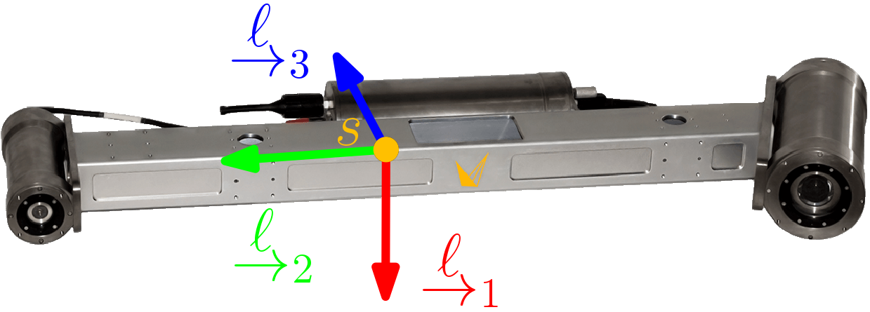
Figure 2: The Insight Pro underwater line scanner by Voyis Imaging Inc., showing the approximate location of datum point $s$ and sensor reference frame ${\mathcal{F}_{\ell}}$. The baseline between the line projector (left) and the camera (right) is approximately $1\text{\,}\mathrm{m}$.

Subsea laser line scanners, such as those developed by the University of Girona [15] and Voyis Imaging Inc. (Figure 2), use optical triangulation to measure high-resolution 2D profiles of underwater environments. A review of the state-of-the-art in underwater optical scanning may be found in [16]. This work considers the problem of laser-to-INS extrinsic calibration using the Voyis Insight Pro laser scanner (Figure 2). This sensor emits a pulsed laser swath with a beam angle of $50\text{\,}\deg$, and uses an optical camera to record 2D laser profiles at a frequency of up to $80\text{\,}\mathrm{Hz}$. To generate 3D point-cloud “submaps” in the world frame, laser measurements ${\mbf{r}^{p_{i}s}_{\ell}\in\mathbb{R}^{3}}$ are registered to sections of the vehicle trajectory via

$$\begin{bmatrix}\mbf{r}^{p_{i}w}_{a}\\ 1\end{bmatrix}=\mbf{T}^{zw}_{ab}\,\mbf{T}^{sz}_{b\ell}\begin{bmatrix}\mbf{r}^{p_{i}s}_{\ell}\\ 1\end{bmatrix},$$ (13)

where extrinsic matrix ${\mbf{T}^{sz}_{b\ell}\in SE(3)}$ captures the static pose of the laser relative to the INS. Interpolating the vehicle trajectory at measurement time $t_{i}$ is done via [17, §2.4]

$$\mbf{T}_{i}=\mbf{T}_{k}\exp\left(\left(\tfrac{t_{i}-t_{k}}{t_{k+1}-t_{k}}\right)\log\left(\mbf{T}^{-1}_{k}\mbf{T}_{k+1}\right)\right),$$ (14)

with ${t_{k}<t_{i}<t_{k+1}}$ and, for example, ${\mbf{T}_{i}\leftarrow\mbf{T}^{z_{i}w}_{ab_{i}}}$. The resulting point-cloud submap is ${\mathcal{P}=\{\mbf{r}^{p_{i}w}_{a}\}^{P}_{i=1}}$.

III Methodology

This section developes three novel algorithms for laser-to-vehicle extrinsic calibration with a Doppler-velocity log (DVL)-aided INS (DVL-INS). Reprojection errors are first defined between pairs of 3D keypoints detected throughout $N$ laser scans. Tikhonov regularization is then used to address low-observability calibration scenarios often encountered with large, rotationally stable underwater vehicles. Three algorithms are derived for laser-to-INS extrinsic calibration subject to different assumptions on the quality of the vehicle trajectory estimate. These assumptions are summarized in Table I.

Note that reliable keypoint extraction (Section III-A) depends heavily on access to a reasonable prior laser-to-INS extrinsic estimate $\hat{\mbf{T}}^{sz}_{b\ell}$. In practice this is a fair assumption, as a prior estimate can almost always be obtained from a CAD model or even from on-site photographs and hand measurements. The certainty of these measurements can then be quantified in the weighting placed on the Tikhonov regularization term. This is discussed in Section III-C.

III-A Extracting 3D Keypoints from Laser Submaps

The calibration algorithms developed in Section III-D minimize a sum of squared reprojection errors defined between pairs of 3D keypoints detected in the $N$ laser scans. To obtain a set of inlier matches between the different scans, 3D SIFT keypoints [18] ${\mbf{r}^{qw}_{a}\in\mathbb{R}^{3}}$ are detected and matched using the TEASER++ coarse alignment algorithm [19] on the basis of FPFH feature correspondences [20]. Failed alignments may be detected though comparison to the INS attitude estimate. Table II provides a summary of the relevant parameters, which were selected after a small amount of tuning to produce good results on the structured datasets studied in this work. The result of this operation is a set of $M$ inlier correspondences between pairs of detected keypoints, with each correspondence allowing for the formulation of one reprojection error $\mbf{e}_{j}$. The formulation of this error is discussed in the next section.

TABLE II: Keypoint detection and matching parameters

Operation	Description
Downsampling	Subsample on $5\text{\,}\mathrm{cm}$ grid
Normal vectors	40 nearest neighbors
Keypoints	3D SIFT [18], PCL v1.9 implementation
Features	FPFH [20], PCL v1.9 implementation
Feature matching	TEASER++ [19], 10 putative matches

III-B Defining and Minimizing Reprojection Errors

Consider Figure 3, in which keypoint submaps $\mathcal{Q}_{1}$ and $\mathcal{Q}_{2}$ are generated according to (13) for two overlapping sections of the vehicle trajectory. For the $j^{\textrm{th}}$ inlier correspondence between keypoints ${\mbf{r}^{q_{1}w}_{a}\!\in\mathcal{Q}_{1}}$ and ${\mbf{r}^{q_{2}w}_{a}\!\in\mathcal{Q}_{2}}$, the reprojection error is

$$\mbf{e}_{j}(\mbf{T}^{sz}_{b\ell})= \ \mbf{r}^{q_{1}w}_{a}-\mbf{r}^{q_{2}w}_{a}$$

$$= \ \mbf{H}\!\left(\mbf{T}^{z_{1}w}_{ab_{1}}\,\mbf{T}^{sz}_{b\ell}\,\mbf{u}^{q_{1}s}_{\ell}-\mbf{T}^{z_{2}w}_{ab_{2}}\,\mbf{T}^{sz}_{b\ell}\,\mbf{u}^{q_{2}s}_{\ell}\right),$$ (15a)

$$\mbf{e}_{j}(\mbf{T})= \ \mbf{H}\big{(}\mbf{T}_{1}\mbf{T}\,\mbf{u}_{1}-\mbf{T}_{2}\mbf{T}\,\mbf{u}_{2}\big{)},$$ (15b)

in which ${\mbf{u}=[\,\mbf{r}^{\mathsf{T}}\ 1]^{\mathsf{T}}}$ is the homogenous form of ${\mbf{r}\in\mathbb{R}^{3}}$, ${\mbf{H}=[\,\mbf{1}\ \ \mbf{0}\,]\in\mathbb{R}^{3\times 4}}$ removes the homogenous component, and where the notation is simplified from (15a) to (15b) such that, for example, ${\mbf{T}_{1}\leftarrow\mbf{T}^{z_{1}w}_{ab_{1}}}$, ${\mbf{T}\leftarrow\mbf{T}^{sz}_{b\ell}}$, and ${\mbf{u}_{1}\leftarrow\mbf{u}^{q_{1}s}_{\ell}}$.

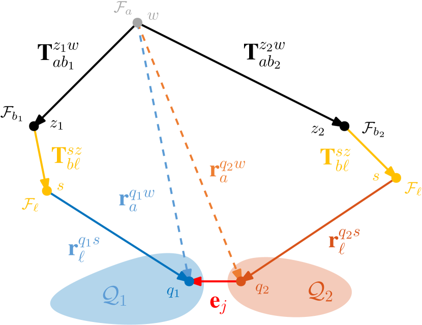
Figure 3: Defining a reprojection error between matched keypoints $\mbf{r}^{q_{1}w}_{a}$ and $\mbf{r}^{q_{2}w}_{a}$. Vehicle poses are shown in black. The design variable is the laser-to-INS extrinsics.

Next, the Jacobians ${\mbf{F}_{j}=\frac{\partial\mbf{e}_{j}}{\partial\bm{\xi}}\big{|}_{\bar{\mbf{T}}}}$ are obtained by linearizing the error model. Perturbing design variable $\mbf{T}$ in a left-invariant sense, with ${\exp(-\delta\bm{\xi}^{\wedge})\approx(\mbf{1}-\delta\bm{\xi}^{\wedge})}$, (15b) is linearized as

$$\mbf{e}_{j}=\bar{\mbf{e}}_{j}+\underbrace{\mbf{H}\!\left(\mbf{T}_{2}\bar{\mbf{T}}\,\bar{\mbf{u}}_{2}^{\odot}-\mbf{T}_{1}\bar{\mbf{T}}\,\bar{\mbf{u}}_{1}^{\odot}\right)}_{\mbf{F}_{j}}\!\delta\bm{\xi}+\underbrace{\mbf{C}_{1}\bar{\mbf{C}}}_{\mbf{G}_{j}^{1}}\delta\mbf{r}_{1}\underbrace{-\mbf{C}_{2}\bar{\mbf{C}}}_{\mbf{G}_{j}^{2}}\delta\mbf{r}_{2},$$ (16)

in which second-order terms have been ignored and where, for example, ${\mbf{r}_{1}\leftarrow\mbf{r}^{q_{1}w}_{a}}$, ${\mbf{r}_{1}=\bar{\mbf{r}}_{1}+\delta\mbf{r}_{1}}$. Letting, for example, ${\mbf{R}_{1}=\mathrm{E}[\,\delta\mbf{r}_{1}\,\delta\mbf{r}_{1}^{\mathsf{T}}\,]}$ represent the covariance on the first point measurement, and assuming the point measurements are uncorrelated, the covariance on the reprojection error is

$$\mbf{M}_{j}=\mbf{G}^{1}_{j}\,\mbf{R}_{1}(\mbf{G}^{1}_{j})^{\mathsf{T}}+\mbf{G}^{2}_{j}\,\mbf{R}_{2}(\mbf{G}^{2}_{j})^{\mathsf{T}}.$$ (17)

A sensitivity study on simulated data [21, §5.3] suggests that, for practical applications, between six to ten point-cloud submaps are needed, with at least twenty common keypoints identified in each submap. This is easily achieved for the structured shipwreck datasets studied in Section IV, but is also possible in unstructured environments provided the terrain is sufficiently textured to allow for repeatable keypoint identification and matching.

III-C Observability Analysis and Regularization

Underwater inspection vehicles are often rotationally stable by design, with transitory roll and pitch excitation falling within $\pm 3\deg$. As a result, patch test trajectories are largely planar, with some variation in vehicle depth. Unfortunately, the optimization problem defined by Section III-B suffers a lack of observability under planar vehicle motion. This is revealed by expanding the Jacobian $\mbf{F}_{j}$ from (16),

$$\mbf{F}_{j}=\begin{bmatrix}\big{(}\mbf{C}_{1}\bar{\mbf{C}}\,\mbf{r}_{1}^{\times}-\mbf{C}_{2}\bar{\mbf{C}}\,\mbf{r}_{2}^{\times}\big{)}&\color[rgb]{1,0,0}{\big{(}\mbf{C}_{2}-\mbf{C}_{1}\big{)}}\color[rgb]{0,0,0}\,\bar{\mbf{C}}\end{bmatrix}.$$ (18)

Owing to the error definition and the peculiarity of the $(\cdot)^{\odot}$ operator (6), $\mbf{F}_{j}$ contains a difference in DCMs, highlighted in red in (18). Under approximately planar vehicle motion, the red terms in (18) become

$$\color[rgb]{1,0,0}{\mbf{C}_{2}-\mbf{C}_{1}}\color[rgb]{0,0,0}\approx\begin{bmatrix}\bm{C}_{2}&\bm{\delta}_{2}\\ \bm{\delta}_{2}^{\mathsf{T}}&1-\delta_{2}\end{bmatrix}-\begin{bmatrix}\bm{C}_{1}&\bm{\delta}_{1}\\ \bm{\delta}_{1}^{\mathsf{T}}&1-\delta_{1}\end{bmatrix}\approx\begin{bmatrix}\mbf{D}&\bm{\delta}\\ \bm{\delta}^{\mathsf{T}}&\delta\end{bmatrix},$$ (19)

where ${\bm{C}_{i}\in SO(2),i=1,2}$ and with ${\bm{\delta}\in\mathbb{R}^{2}}$, $\delta$ some small values. In a typical vehicle integration the Voyis Insight Pro scanner is oriented directly downward, and the initial mean attitude estimate $\tilde{\mbf{C}}_{b\ell}$ is simply an ENU-to-NED principal rotation. This means the last three columns of $\mbf{F}_{j}$ are initially

$$(\mbf{C}_{2}-\mbf{C}_{1})\,\tilde{\mbf{C}}=\begin{bmatrix}\mbf{D}&\bm{\delta}\\ \bm{\delta}^{\mathsf{T}}&\delta\end{bmatrix}\begin{bmatrix}0&1&0\\ 1&0&0\\ 0&0&-1\end{bmatrix}=\begin{bmatrix}\star&-\bm{\delta}\\ \star&-\delta\end{bmatrix},$$ (20)

where the $\star$ entries are assumed to be full column rank. Under approximately planar vehicle motion $\bm{\delta}$ and $\delta$ are small, the full Jacobian matrix ${\mbf{F}=[\,\begin{matrix}\mbf{F}_{1}^{\mathsf{T}}&\cdots&\mbf{F}_{M}^{\mathsf{T}}\end{matrix}\,]^{\mathsf{T}}}$ no longer has full numerical column rank, and component $\delta\rho_{3}$ of the state update will no longer be observable. This same observability issue is noted in [8, 3, 9] for extrinsic calibration on ground vehicles.

In contrast to the observability-aware update approach used in [10], this work uses Tikhonov regularization [22, §6.3.2] to ensure the state update $\delta\bm{\xi}_{\star}$ remains a reasonable size when $\mbf{F}$ is poorly conditioned. Tikhonov regularization is analogous to including a prior measurement ${\check{\mbf{T}}_{0}=\tilde{\mbf{T}}_{0}\exp(-\delta\bm{\eta}_{0}^{\wedge})}$ on the laser-to-INS extrinsics $\mbf{T}$, leading to the objective function

$$J_{1}(\mbf{T})=\frac{1}{2}\Big{(}\|\mbf{e}_{0}(\mbf{T})\|^{2}_{\mbf{P}_{0}^{-1}}+\sum^{M}_{j=1}\|\mbf{e}_{j}(\mbf{T})\|^{2}_{\mbf{M}_{j}^{-1}}\Big{)}.$$ (21)

The (left-invariant) prior error $\mbf{e}_{0}(\mbf{T})$ takes the form

$$\bar{\mbf{e}}_{0}= \ \log(\bar{\mbf{T}}^{-1}\tilde{\mbf{T}}_{0})^{\vee},$$ (22a)

$$\mbf{e}_{0}= \ \bar{\mbf{e}}_{0}+\underbrace{\mbf{J}^{\ell}(\bar{\mbf{e}}_{0})^{-1}}_{\mbf{F}_{0}}\delta\bm{\xi}\underbrace{-\mbf{J}^{\textrm{r}}(\bar{\mbf{e}}_{0})^{-1}}_{\mbf{G}_{0}}\delta\bm{\eta}_{0},$$ (22b)

where $\mbf{J}^{\ell}$ and $\mbf{J}^{\textrm{r}}$ are, respectively, the left and right Jacobians of $SE(3)$ [12, §7.1.5], and where parameter ${\bm{\Sigma}_{0}=\mathrm{E}[\,\delta\bm{\eta}_{0}\,\delta\bm{\eta}_{0}^{\mathsf{T}}\,]}$ is the covariance on the prior measurement, with ${\mbf{P}_{0}=\mbf{G}_{0}\bm{\Sigma}_{0}\mbf{G}_{0}^{\mathsf{T}}}$. This parameter is tuned according to the certainty of the prior measurement, for example whether the measurement is from a customer metrology report or is taken by hand in the field.

Tikhonov regularization allows for reasonably-sized updates along poorly observable dimensions. This keeps the problem well-conditioned while still allowing it to incorporate information from any residual pitch or roll excitation that may be present in the vehicle trajectory estimate. This approach is different from the observability-aware update used in [10], which performs a truncated SVD to simply reject updates in poorly observable dimensions. In the current application, such an approach may entail that the third component of $\mbf{r}^{sz}_{b}$ is never updated from its prior value, despite weakly observable evidence in the calibration data that an update is merited.

III-D Three Algorithms for Laser-to-INS Extrinsic Calibration

Three algorithms for laser-to-INS extrinsic calibration are presented in this section, subject to increasingly weaker assumptions on the quality of the vehicle trajectory estimate (Table I). This allows for good extrinsic calibration in a wide range of practical scenarios.

III-D1 Algorithm 1: Perfect Navigation

Algorithm 1 assumes the vehicle navigation is perfect, and only optimizes over the laser-to-INS extrinsics $\mbf{T}^{sz}_{b\ell}$. This assumption could be valid in scenarios where high-precision navigational aiding is available, for example a long-baseline (LBL) acoustic array, or GPS in surface applications. The result is a nonlinear least-squares optimization problem of the form (8), with $J(\bm{\mathcal{X}})$ simply replaced by the objective function $J_{1}(\mbf{T})$ from (21).

III-D2 Algorithm 2: Good Local Navigation with Global Drift

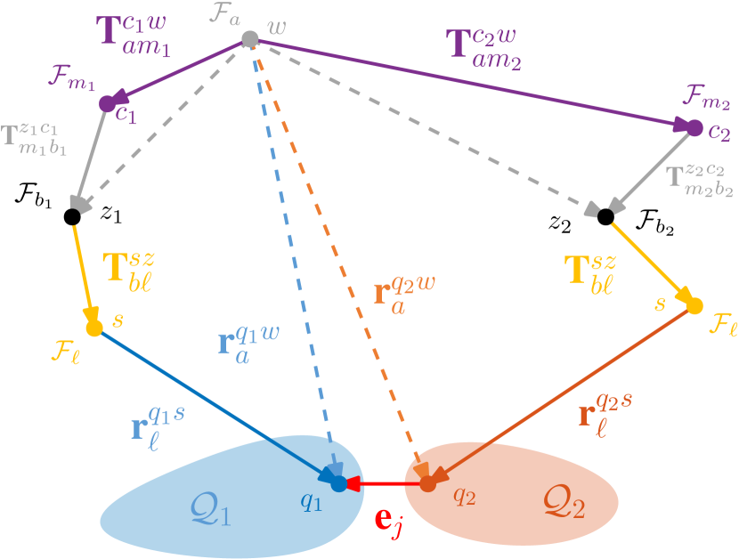
Figure 4: Defining a reprojection error $\mbf{e}_{j}$ for Algorithm 2, which allows for global submap drift. Comparison to Figure 3 shows the individual vehicle poses (black) have been replaced with the central submap poses and rigid offsets. The design variables are the laser-to-INS extrinsics and the central submap poses.

A more realistic assumption for underwater navigation is good local navigation with global drift. In this scenario an underwater vehicle is equipped with a high-quality DVL-INS, and either dead-reckons or receives intermittent correction from a lower-precision acoustic sensor such as a surface-mounted ultrashort baseline (USBL) array. The resulting point-cloud submaps are assumed to be locally rigid, but are allowed some degree of global pose refinement to correct for gross navigation errors. Algorithm 2 accounts for this by including the central poses of the $N$ submaps as design variables, with a prior term to control the degree of global pose correction.

Consider Figure 4, where the reprojection error $\mbf{e}_{j}$ is redefined in terms of both the laser-to-INS extrinsics $\mbf{T}^{sz}_{b\ell}$, shown in yellow, and the central submap poses $\mbf{T}^{cw}_{am}$, shown in purple. The central poses are chosen to be the poses in each submap that lie nearest, in a Euclidean sense, to the identified trajectory crossing. For readability, the central poses are identified by the vehicle datum $c$ and the vehicle reference frame ${\mathcal{F}_{m}}$. The relative poses $\mbf{T}^{zc}_{mb}$, shown in grey in Figure 4, parameterize each vehicle pose within a submap relative to the central submap pose at the time each keypoint was measured by the laser. To ensure the submap remains rigid, these relative poses are precomputed and are treated as parameters in the optimization.

To derive the the ingredients needed for batch optimization (11), first use Figure 4 to redefine the reprojection error as

$$\mbf{e}_{j}(\mbf{T}^{sz}_{b\ell},\mbf{T}^{c_{1}w}_{am_{1}},\mbf{T}^{c_{2}w}_{am_{2}})= \ \mbf{r}^{q_{1}w}_{a}-\mbf{r}^{q_{2}w}_{a}$$

$$\begin{split}=&\ \mbf{H}\Big{(}\mbf{T}^{c_{1}w}_{am_{1}}\,\mbf{T}^{z_{1}c_{1}}_{m_{1}b_{1}}\,\mbf{T}^{sz}_{b\ell}\,\mbf{u}^{q_{1}s}_{\ell}\\ &\ -\mbf{T}^{c_{2}w}_{am_{2}}\,\mbf{T}^{z_{2}c_{2}}_{m_{2}b_{2}}\,\mbf{T}^{sz}_{b\ell}\,\mbf{u}^{q_{2}s}_{\ell}\Big{)},\end{split}$$ (23a)

$$\mbf{e}_{j}(\mbf{T},\mbf{T}_{1},\mbf{T}_{2})= \ \mbf{H}\big{(}\mbf{T}_{1}\,\tilde{\mbf{T}}_{1}\mbf{T}\,\mbf{u}_{1}-\mbf{T}_{2}\,\tilde{\mbf{T}}_{2}\mbf{T}\,\mbf{u}_{2}\big{)},$$ (23b)

in which the homogenous form $\mbf{u}$ is used for the point measurements and where the notation is simplified from (23a) to (23b) such that, for example, ${\mbf{T}_{1}\leftarrow\mbf{T}^{c_{1}w}_{am_{1}}}$, ${\tilde{\mbf{T}}_{1}\leftarrow\mbf{T}^{z_{1}c_{1}}_{m_{1}b_{1}}}$, ${\mbf{T}\leftarrow\mbf{T}^{sz}_{b\ell}}$, and ${\mbf{u}_{1}\leftarrow\mbf{u}^{q_{1}s}_{\ell}}$. Perturbing design variables $\mbf{T}$, $\mbf{T}_{1}$, and $\mbf{T}_{2}$ in a left-invariant sense, with ${\exp(-\delta\bm{\xi}^{\wedge})\approx(\mbf{1}-\delta\bm{\xi}^{\wedge})}$, (23b) is linearized as

$$\mbf{e}_{j}= \ \bar{\mbf{e}}_{j}+\underbrace{\mbf{H}\big{(}\bar{\mbf{T}}_{2}\,\tilde{\mbf{T}}_{2}\bar{\mbf{T}}\,\bar{\mbf{u}}_{2}^{\odot}-\bar{\mbf{T}}_{1}\,\tilde{\mbf{T}}_{1}\bar{\mbf{T}}\,\bar{\mbf{u}}_{1}^{\odot}\big{)}}_{\mbf{F}_{j}}\delta\bm{\xi}$$

$$\ \underbrace{-\mbf{H}\big{(}\bar{\mbf{T}}_{1}\big{(}\tilde{\mbf{T}}_{1}\bar{\mbf{T}}\,\bar{\mbf{u}}_{1}\big{)}^{\odot}\big{)}}_{\mbf{F}^{1}_{j}}\delta\bm{\xi}_{1}+\underbrace{\mbf{H}\big{(}\bar{\mbf{T}}_{2}\big{(}\tilde{\mbf{T}}_{2}\bar{\mbf{T}}\,\bar{\mbf{u}}_{2}\big{)}^{\odot}\big{)}}_{\mbf{F}^{2}_{j}}\delta\bm{\xi}_{2}$$

$$\ +\underbrace{\bar{\mbf{C}}_{1}\tilde{\mbf{C}}_{1}\bar{\mbf{C}}}_{\mbf{G}^{1}_{j}}\delta\mbf{r}_{1}\underbrace{-\bar{\mbf{C}}_{2}\tilde{\mbf{C}}_{2}\bar{\mbf{C}}}_{\mbf{G}^{2}_{j}}\delta\mbf{r}_{2},$$ (24)

where second-order terms are again ignored. Following the same substitutions and assumptions used in Section III-B, the covariance on the reprojection error is given by (17). Incorporating the Tikhonov regularization term from (22) and placing prior measurements on each of the $N$ submaps, the objective function for Algorithm 2 becomes

$$J_{2}(\bm{\mathcal{X}})\!=\!\frac{1}{2}\Big{(}\!\|\mbf{e}_{0}(\mbf{T})\|^{2}_{\mbf{P}_{0}^{-1}}+\sum^{N}_{i=1}\|\mbf{e}_{i}(\mbf{T}_{i})\|^{2}_{\mbf{P}_{i}^{-1}}+\sum^{M}_{j=1}\|\mbf{e}_{j}(\bm{\mathcal{X}}_{j})\|^{2}_{\mbf{M}_{j}^{-1}}\!\Big{)},$$ (25)

where the design variables are ${\bm{\mathcal{X}}=\{\mbf{T}^{sz}_{b\ell},\mbf{T}^{c_{1}w}_{am_{1}},\ldots,\mbf{T}^{c_{N}w}_{am_{N}}\}}$, and where user-defined parameter $\bm{\Sigma}_{i}$ controls the strength of the global submap priors, with ${\mbf{P}_{i}=\mbf{G}_{i}\bm{\Sigma}_{i}\mbf{G}_{i}^{\mathsf{T}}}$ (see (22)).

III-D3 Algorithm 3: Poor Navigation

Algorithm 3 assumes the local vehicle trajectory estimate is of poor quality, for example when the vehicle is equipped with a MEMS-based IMU. In this scenario the rigid submap assumption used in Algorithm 2 may no longer be valid, leading to the general case of laser-to-INS extrinsic calibration using flexible submaps.

Consider Figure 5, where the $i^{\textrm{th}}$ flexible submap is constructed using $K_{i}$ vehicle poses, ${\mbf{T}_{k}=\mbf{T}^{z_{k}w}_{ab_{k}},k=1,\ldots,K_{i}}$. The submap is globally constrained by the exteroceptive error terms $\mbf{e}^{\textrm{y}}$, but is allowed to adjust its shape through the interoceptive error terms $\mbf{e}^{\textrm{u}}$ linking adjacent poses. This adaptability will be needed in situations where the short-term navigation drift within each submap is no longer negligible, for example when using low-cost underwater vehicles.

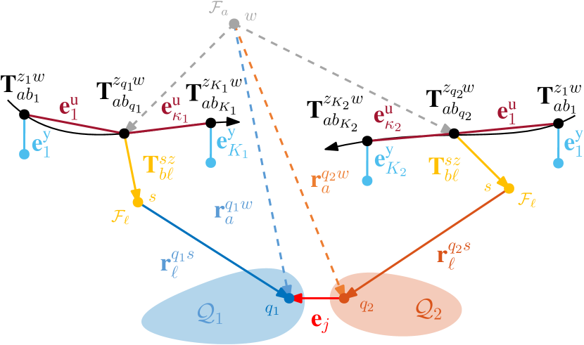
Figure 5: A depiction of Algorithm 3, with exteroceptive errors placed on the DVL-INS poses and interoceptive errors linking all DVL-INS and measurement poses, both shown in black. The design variables include the laser-to-INS extrinsics as well as the intrinsic and extrinsic variables.

The experimental results in this work use data from a DVL-INS, which does not provide access to raw interoceptive measurements but instead provides pose measurements ${\check{\mbf{T}}_{k}\in SE(3)}$. As a result, this work assumes a white-noise-on-acceleration (WNOA) vehicle motion prior [23], leading to WNOA interoceptive errors of the form

$$\mbf{e}_{k}^{\textrm{w}}=\log\Big{(}\mbf{T}_{k}^{-1}\big{(}\mbf{T}_{k-1}\exp\big{(}\delta t_{k-1}\bm{\varpi}^{\wedge}_{k-1}\big{)}\big{)}\Big{)}^{\vee},\vspace{-3pt}$$ (26)

with $\delta t$ a time increment and ${\bm{\varpi}\in\mathbb{R}^{6}}$ the generalized velocity. See [24] for a comprehensive derivation. Additionally, relative pose errors of the form

$$\mbf{e}_{k}^{\textrm{r}}=\log\left(\mbf{T}_{k}^{-1}\left(\mbf{T}_{k-1}\check{\mbf{T}}^{-1}_{k-1}\check{\mbf{T}}_{k}\right)\right)^{\vee}\vspace{-3pt}$$ (27)

were found in [24] to retain some rigidity throughout the submaps, allowing global corrections to propagate more easily. Finally, prior pose errors of the form

$$\mbf{e}^{\textrm{p}}_{k}=\log\big{(}\mbf{T}_{k}^{-1}\check{\mbf{T}}_{k}\big{)}^{\vee}\vspace{-3pt}$$ (28)

are constructed for each vehicle pose using the DVL-INS measurements. Incorporating reprojection errors $\mbf{e}_{j}$, the prior pose errors $\mbf{e}^{\textrm{p}}_{k}$ and interoceptive errors $\mbf{e}_{k}^{\textrm{w}}$ and $\mbf{e}_{k}^{\textrm{r}}$ from above, and the Tikhonov regularization term from (22), the objective function for Algorithms 3 is

$$\begin{split}J_{3}(\bm{\mathcal{X}})=&\ \frac{1}{2}\Big{(}\sum^{M}_{j=1}\|\mbf{e}_{j}(\bm{\mathcal{X}}_{j})\|_{\mbf{M}_{j}^{-1}}^{2}+\sum^{N}_{i=1}\Big{(}\sum^{K_{i}}_{k=1}\|\mbf{e}^{\textrm{p}}_{k}(\mbf{T}_{k})\|^{2}_{\mbf{P}_{k}^{-1}}\\ &+\sum^{\kappa_{i}}_{k=1}\Big{(}\|\mbf{e}^{\textrm{w}}_{k}(\bm{\mathcal{X}}^{\textrm{w}}_{k})\|^{2}_{\mbf{Q}_{k}^{-1}}+\|\mbf{e}^{\textrm{r}}_{k}(\bm{\mathcal{X}}^{\textrm{r}}_{k})\|^{2}_{\mbf{R}_{k}^{-1}}\Big{)}\Big{)}+\|\mbf{e}_{0}\|^{2}_{\mbf{P}_{0}^{-1}}\Big{)}.\end{split}$$ (29)

Unpacking (29), the prior pose error covariance $\mbf{P}_{k}$ is generated from the DVL-INS measurement covariance $\bm{\Sigma}_{k}$ (see (22)), while covariances $\mbf{Q}_{k}$ and $\mbf{R}_{k}$ incorporate user-defined parameters (see [24]). The limit ${\kappa_{i}=K_{i}+Q_{i}-1}$ of the last sum reflects the fact that the interoceptive errors must incorporate both the DVL-INS vehicle poses $\mbf{T}_{k}$ as well as the keypoint measurement poses $\mbf{T}_{q}$, with $Q_{i}$ the total number of keypoints detected in the $i^{\textrm{th}}$ submap. The set of design variables $\bm{\mathcal{X}}$ in Algorithm 3 is quite large, incorporating the laser-to-INS extrinsics, the vehicle poses at the DVL-INS timestamps $t_{k}$ as well as the keypoint timestamps $t_{q}$, and all intervening generalized velocities.

IV Results

The developed algorithms are used for laser-to-INS extrinsic calibration on two experimental datasets: a small shipwreck dataset collected by a surface vessel, and a laser model of the Endurance shipwreck collected by a SAAB Sabertooth AUV during the Endurance22 expedition [25].

IV-A Experimental Results: Wiarton Shipwreck

In this section, all three algorithms are used for laser-to-INS extrinsic calibration on a surface vessel. Figure 6(a) shows the sensor payload on the bow of the vessel, with a Sonardyne SPRINT-Nav DVL-INS and Voyis Insight Pro laser scanner highlighted. The vessel scanned a small shipwreck in shallow water during a field deployment to Colpoy’s Bay, located in Wiarton, Ontario, Canada. Figure 6(b) shows the main shipwreck structure and eight sections of the vehicle trajectory. The full details of this field deployment may be found in [24].

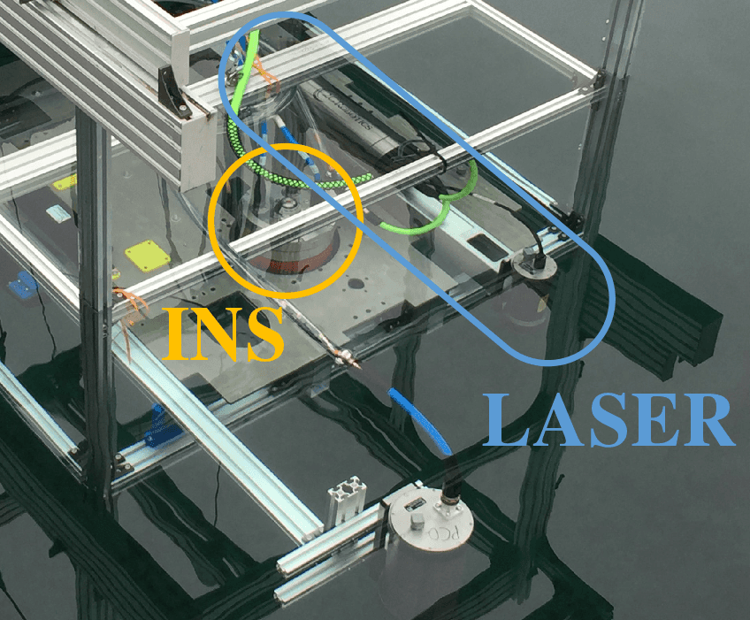
(a) Sensor payload

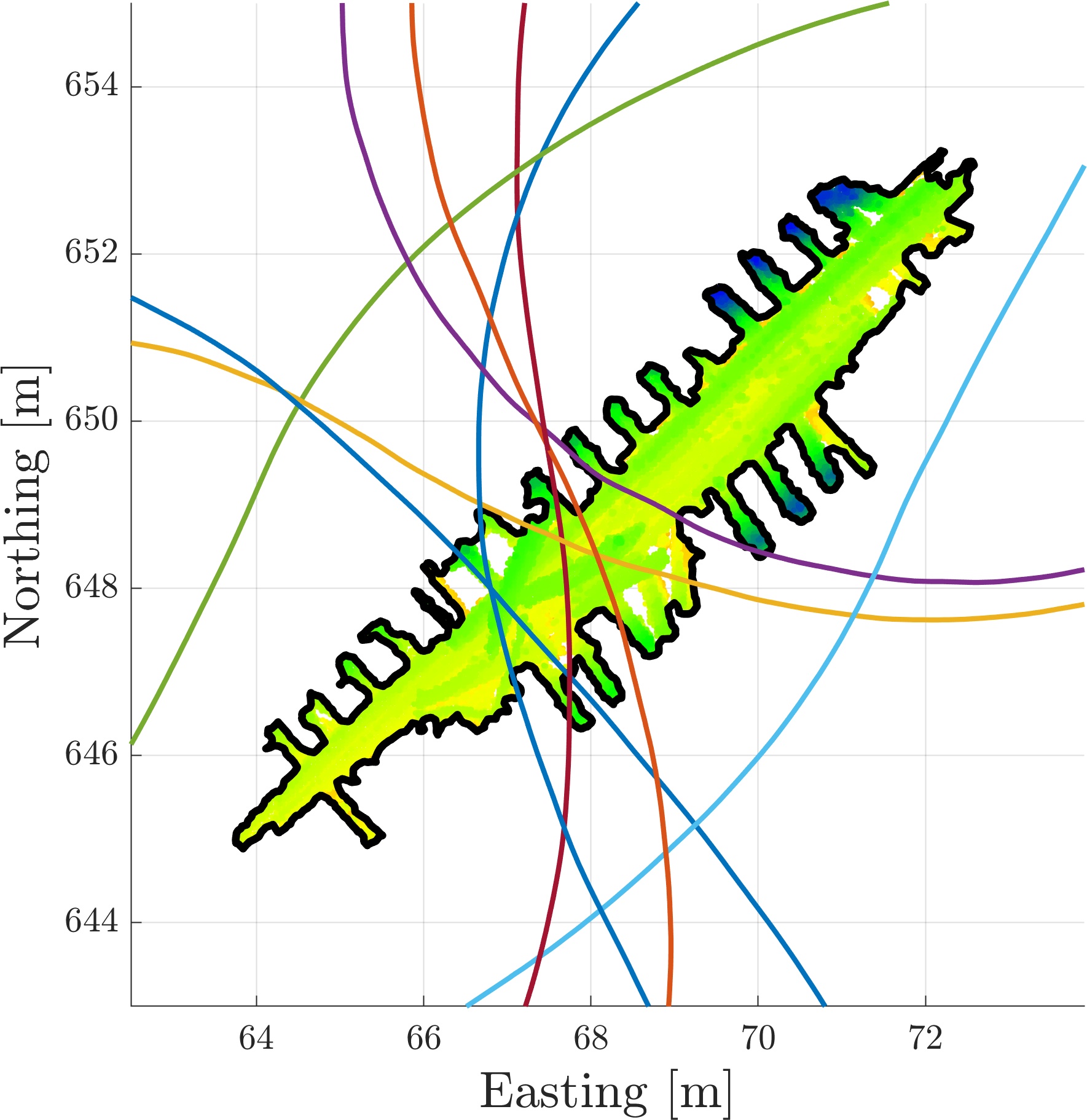
(b) Wreck and passes

Figure 6: Field testing with Voyis Imaging Inc. The surface vessel payload is shown in Figure 6(a), while the shipwreck structure is shown in Figure 6(b). Individual vehicle passes over the wreck area are highlighted in different colours.

A total of ${N=8}$ point-cloud submaps are first constructed from a GPS-aided DVL-INS trajectory estimate. Reprojection errors $\mbf{e}_{j}$ are formed between the submaps from inlier keypoint matches identified by TEASER++, and extrinsic optimization is performed using Algorithms 1-3. The initial mean laser-to-INS extrinsic estimate $\tilde{\mbf{T}}^{sz}_{b\ell}$ is obtained from a CAD model of the sensor rig, and the prior measurement covariance is set to

$$\bm{\Sigma}_{0}=\operatorname{blkdiag}(\sigma^{\phi}_{0}\,\mbf{1},\,\sigma^{\rho}_{0}\,\mbf{1})^{2},$$ (30)

with ${\sigma^{\phi}_{0}=$1\text{\,}\deg$}$ and ${\sigma^{\rho}_{0}=$5\text{\,}\mathrm{cm}$}$. The global submap pose covariance $\bm{\Sigma}_{i}$ used in Algorithm 2 follows the same parameter structure, with ${\sigma^{\phi}_{i}=$1\text{\,}\deg$}$ ${\sigma^{\rho}_{i}=$25\text{\,}\mathrm{cm}$}$.

Updates to the laser-to-INS extrinsics are reported as

$$\delta\bm{\phi}_{\ell b}= \ \log(\tilde{\mbf{C}}^{\mathsf{T}}\mbf{C}_{\star})^{\vee},$$ (31a)

$$\delta\mbf{r}^{sz}_{b}= \ \mbf{r}_{\star}-\tilde{\mbf{r}}.$$ (31b)

Reporting the updates on ${SO(3)\times\mathbb{R}^{3}}$ means the position updates are resolved in the body frame of the vehicle, which is easier to interpret. Updates produced by the three algorithms are reported in Table III.

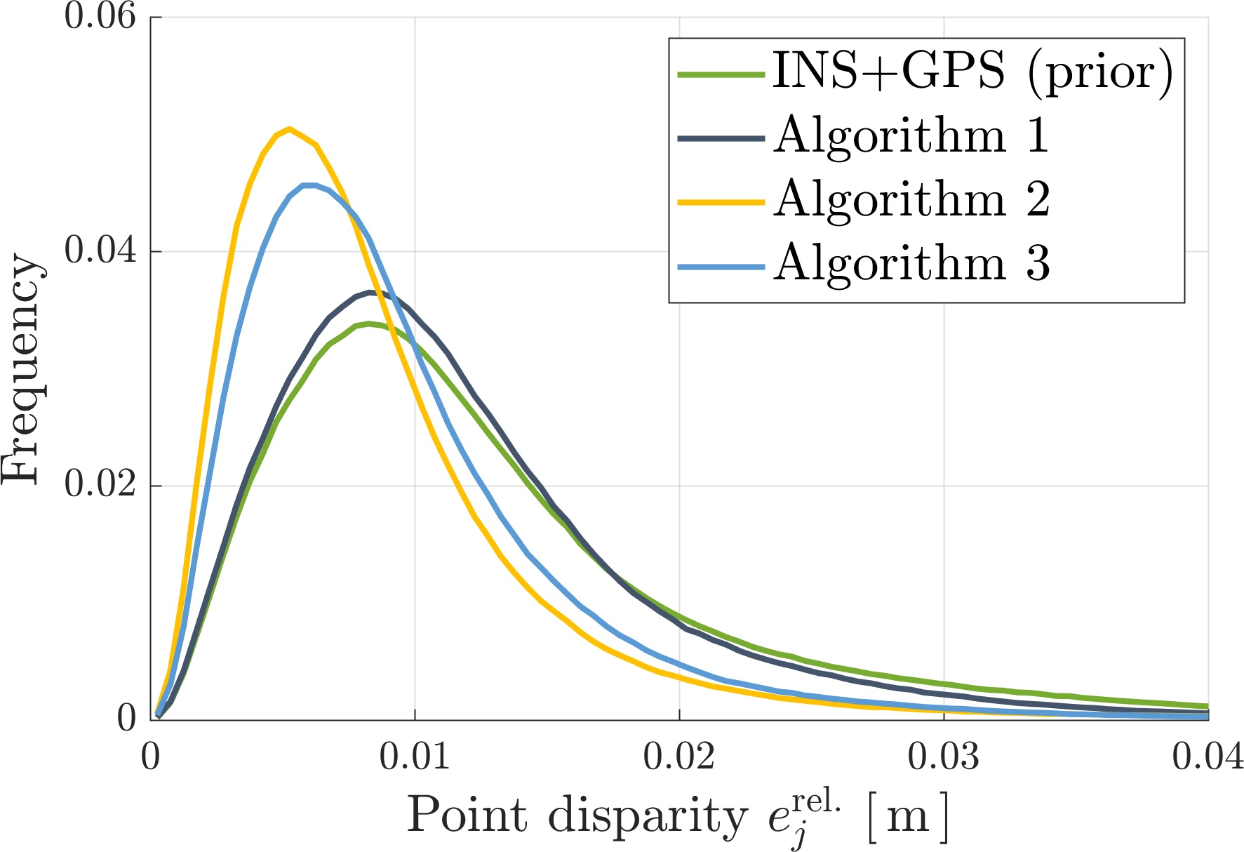
Figure 7: Empirical PDFs on the point disparity error for the Wiarton shipwreck dataset. The “INS+GPS” result is from [24], while Algorithms 1-3 are the methods from Section III-D.

TABLE III: Change from CAD values for Wiarton extrinsics

Alg.	$\|\delta\bm{\phi}\|\,\left[\deg\right]$	$\delta r^{1}_{b}\,\left[$\text{\,}\mathrm{cm}$\right]$	$\delta r^{2}_{b}\,\left[$\text{\,}\mathrm{cm}$\right]$	$\delta r^{3}_{b}\,\left[$\text{\,}\mathrm{cm}$\right]$
1	$0.17\text{\,}$	$0.77\text{\,}$	-3.44	-3.80
2	$0.18\text{\,}$	-$3.2010-3\text{\,}$	-$0.32\text{\,}$	$4.1010-3\text{\,}$
3	$0.18\text{\,}$	-$6.8910-2\text{\,}$	-1.92	$7.2710-2\text{\,}$

Results are also assessed by computing the point disparity errors [1] in the posterior point-cloud submaps. For each point, the point disparity error is simply the Euclidean distance to the closest point in any of the other ${N-1}$ submaps, with a low average disparity error indicating a well-aligned, “crisp” point-cloud map. Figure 7 shows empirical probability density functions (PDFs) for the three calibration algorithms as well as for the prior GPS-aided “INS+GPS” trajectory from [24].

Together, the results make a strong case for the applicability of Algorithm 2 in this particular context. Algorithm 2 is the most successful in reducing the point disparity error, as seen by comparing the yellow and green curves in Figure 7. Additionally, the small updates suggested by Algorithm 2 in Table III are consistent with mounting tolerances for a CAD-designed, machined plate (Figure 6(a)). The improved performance of Algorithm 2 over Algorithm 1, which assumes a perfect navigation estimate, suggests a possible bias in the post-processed GPS data, perhaps from an error in the GPS-to-INS extrinsic estimate. The improved performance of Algorithm 2 over Algorithm 3 suggests the minimization of the cost $J_{3}(\bm{\mathcal{X}})$ from (29) favoured the reduction of the squared prior errors $\mbf{e}^{\textrm{p}}_{k}$ and WNOA errors $\mbf{e}^{\textrm{w}}_{k}$ over the reduction of the squared point disparity errors $\mbf{e}_{j}$. Further tuning of the $\mbf{P}_{k}$ and $\mbf{Q}_{k}$ covariance matrices may lead to improved performance for Algorithm 3 in scenarios involving low-cost navigation systems.

IV-B Experimental Results: Wreck of the Endurance

The Endurance, captained by Sir Ernest Shackleton, sank in 1915 during an ill-fated attempt to cross Antarctica. The story that followed is a well-known case study in stoicism and leadership, whereby Shackleton and all 27 members of his crew survived following an epic trial of ocean navigation [26]. The ship was not as fortunate, and sank in the Weddell Sea on Nov. 21, 1915 after being crushed by ice. Given the harsh and extremely remote environment, the exact location of the wreck remained a mystery for over one hundred years.

The Endurance22 expedition, organized by the Falklands Maritime Heritage Trust, was launched in Feb. 2022 with the primary goal of locating the wreck of the Endurance. Once located, a SAAB Sabertooth AUV was used to inspect the wreck site. The vehicle was equipped with a Sonardyne SPRINT-Nav DVL-INS, a USBL beacon, a depth sensor, and an Insight Pro laser line scanner from Voyis Imaging Inc.

The wreck site was located at a depth of $3\text{\,}\mathrm{km}$. At this range, USBL signals from the surface vessel were not precise enough to aid navigation, and the thick layer of sea ice made the deployment of an LBL array impossible. The AUV trajectory was therefore dead-reckoned for the duration of the inspection.

As part of the efforts to construct a 3D point-cloud model of the wreck site, Algorithm 2 is used to calibrate the laser-to-INS extrinsics using a dedicated patch test dataset with ${N=7}$ submaps. The assumptions behind Algorithm 2 make sense in this context, where high-quality dead-reckoning is available and localizing measurements are unavailable.

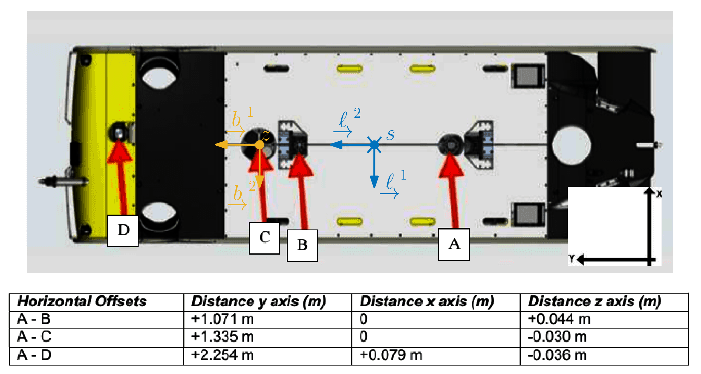
Figure 8: A metrology report for the SAAB Sabertooth AUV used on the Endurance22 expedition, modified to show the pose of the laser relative to the DVL-INS. Modified with permission from the Falklands Maritime Heritage Trust.

A good initial guess is provided by the AUV metrology report, shown in Figure 8. Though this report was generated using high-precision photogrammetry, the laser datum is inaccessible behind the AUV housing and its exact location is somewhat unclear. The prior displacement measurement $\tilde{\mbf{r}}^{sz}_{b}$ is taken to lie midway between points A and B in Figure 8, resulting in

$$\tilde{\mbf{r}}^{sz}_{b}=\begin{bmatrix}-0.80&0&0\end{bmatrix}^{\mathsf{T}},$$ (32)

while an ENU-to-NED principal rotation is taken as the prior attitude measurement $\tilde{\mbf{C}}_{b\ell}$. The parameter values from (30) for the prior extrinsic and global submap pose measurements are ${\sigma_{0}^{\phi}=\sigma_{i}^{\phi}=$1\text{\,}\deg$}$, ${\sigma^{\rho}_{0}=$0.1\text{\,}\mathrm{m}$}$, and ${\bm{\Sigma}^{\rho}_{i}={\mathrm{diag}}(1^{2},1^{2},(0.1)^{2})\,$\text{\,}\mathrm{m}$}$. The non-isotropic structure of $\bm{\Sigma}^{\rho}_{i}$ reflects greater precision in depth owing to the availability of depth sensor measurements.

After running Algorithm 2, the update to the laser-to-INS extrinsics is computed using (31). A reasonable value of ${\|\delta\bm{\phi}_{\ell b}\|=$0.36\text{\,}\deg$}$ is obtained for the attitude update, while the position update in centimeters is found to be

$$\delta\mbf{r}^{sz}_{b}=\begin{bmatrix}4.68&$-2.5210-3\text{\,}$&$0.14\text{\,}$\end{bmatrix}^{\mathsf{T}}.$$ (33)

Considering Figure 8, the displacement update lies almost perfectly along ${\underrightarrow{{b}}}^{1}$, the main axis of the AUV. The relative position measurement in this dimension was initially unclear, as the laser datum is inaccessible behind the AUV housing. The displacement update makes sense, indicating the scanner is $4.68\text{\,}\mathrm{cm}$ closer to the DVL-INS than initially assumed.

Finally, the quality of the posterior point-cloud map is assessed by computing the point disparity errors for the patch test submaps. The results are visualized as a colourmap in Figure 1. Algorithm 2, which jointly optimizes over both the laser-to-INS extrinsics and the global submap poses, has reduced the median point disparity error from $7.7\text{\,}\mathrm{cm}$ to $0.6\text{\,}\mathrm{cm}$. The posterior point-cloud map provides a strikingly crisp, high-resolution reconstruction of this historic wreck.

V Conclusion

Underwater laser scanners such as the Voyis Insight Pro are increasingly used for high-resolution infrastructure inspection and environmental monitoring. However, reliable laser-to-INS extrinsic calibration remains a challenge on commercial surveys. This work developed three novel algorithms for laser-to-INS calibration using naturally occurring features. All algorithms employ Tikhonov regularization to address low-observability scenarios frequently encountered in practice. Each algorithm makes a different assumption on the quality of the vehicle trajectory estimate, however Algorithm 2, which assumes good local navigation with global drift, proved a good choice for both field datasets. All three algorithms were successfully used on a small shipwreck dataset from Wiarton, Ontario, while Algorithm 2 was used to refine the laser-to-INS extrinsics for the SAAB Sabertooth AUV used on the Endurance22 expedition. Future work will focus on extrinsic calibration for low-cost systems, and on an iterative approach to address instances of poor initialization.

References

- [1] Chris Roman and Hanumant Singh “Consistency Based Error Evaluation for Deep Sea Bathymetric Mapping with Robotic Vehicles” In Proc. IEEE Int. Conf. Robot. and Autom., 2006, pp. 3568–3574 IEEE
- [2] Paul Furgale, Joern Rehder and Roland Siegwart “Unified temporal and spatial calibration for multi-sensor systems” In Proc. IEEE/RSJ Int. Conf. Intell. Robots Syst., 2013, pp. 1280–1286 IEEE
- [3] Zachary Taylor and Juan Nieto “Motion-based calibration of multimodal sensor extrinsics and timing offset estimation” In IEEE Trans. Robot. 32.5 IEEE, 2016, pp. 1215–1229
- [4] Ashley Napier, Peter Corke and Paul Newman “Cross-calibration of push-broom 2D LIDARs and cameras in natural scenes” In Proc. IEEE Int. Conf. Robot. Autom., 2013, pp. 3679–3684 IEEE
- [5] Will Maddern, Alastair Harrison and Paul Newman “Lost in translation (and rotation): Rapid extrinsic calibration for 2D and 3D LIDARs” In Proc. IEEE Int. Conf. Robot. Autom., 2012, pp. 3096–3102 IEEE
- [6] Haoyang Ye, Yuying Chen and Ming Liu “Tightly coupled 3D lidar inertial odometry and mapping” In Proc. IEEE Int. Conf. Robot. Autom., 2019, pp. 3144–3150 IEEE
- [7] Jiajun Lv et al. “Targetless calibration of LiDAR-IMU system based on continuous-time batch estimation” In Proc. IEEE/RSJ Int. Conf. Intell. Robots Syst., 2020, pp. 9968–9975 IEEE
- [8] Faraz M Mirzaei, Dimitrios G Kottas and Stergios I Roumeliotis “3D LIDAR–camera intrinsic and extrinsic calibration: Identifiability and analytical least-squares-based initialization” In Int. J. Robot. Res. 31.4 SAGE Publications Sage UK: London, England, 2012, pp. 452–467
- [9] Xingxing Zuo et al. “LIC-fusion 2.0: LiDAR-inertial-camera odometry with sliding-window plane-feature tracking” In Proc. IEEE/RSJ Int. Conf. Intell. Robots Syst., 2020, pp. 5112–5119 IEEE
- [10] Jiajun Lv et al. “Observability-Aware Intrinsic and Extrinsic Calibration of LiDAR-IMU Systems” In IEEE Trans. Robot. 38.6 IEEE, 2022, pp. 3734–3753
- [11] Sandipan Das, Ludvig Klinteberg, Maurice Fallon and Saikat Chatterjee “Observability-aware online multi-lidar extrinsic calibration” In IEEE Robot. Autom. Lett. IEEE, 2023
- [12] Timothy D Barfoot “State Estimation for Robotics” Cambridge University Press, 2017
- [13] Joan Sola, Jeremie Deray and Dinesh Atchuthan “A micro Lie theory for state estimation in robotics” In arXiv preprint arXiv:1812.01537, 2018
- [14] Jonathan Arsenault “Practical Considerations and Extensions of the Invariant Extended Kalman Filtering Framework”, 2019
- [15] Albert Palomer, Pere Ridao, Josep Forest and David Ribas “Underwater Laser Scanner: Ray-based Model and Calibration” In IEEE/ASME Trans. Mechatron. 24.5 IEEE, 2019, pp. 1986–1997
- [16] Miguel Castillón, Albert Palomer, Josep Forest and Pere Ridao “State of the art of underwater active optical 3D scanners” In Sensors 19.23 MDPI, 2019, pp. 5161
- [17] Ethan Eade “Lie groups for computer vision”, 2014
- [18] David G Lowe “Distinctive image features from scale-invariant keypoints” In Int. J. Comput. Vis. 60.2 Springer, 2004, pp. 91–110
- [19] Heng Yang, Jingnan Shi and Luca Carlone “TEASER: Fast and Certifiable Point Cloud Registration” In IEEE Trans. Robot. 37.2 Springer, 2020, pp. 314–333
- [20] Radu Bogdan Rusu, Nico Blodow and Michael Beetz “Fast point feature histograms (FPFH) for 3D registration” In Proc. IEEE Int. Conf. Robot. Autom., 2009, pp. 3212–3217 IEEE
- [21] Thomas Hitchcox “Strategies for Subsea Navigation and Mapping Using an Underwater Laser Scanner”, 2023
- [22] Stephen Boyd and Lieven Vandenberghe “Convex Optimization” Cambridge University Press, 2004
- [23] Sean Anderson and Timothy D Barfoot “Full STEAM ahead: Exactly sparse Gaussian process regression for batch continuous-time trajectory estimation on ” In Proc. IEEE/RSJ Int. Conf. Intell. Robots Syst., 2015, pp. 157–164 IEEE
- [24] Thomas Hitchcox and James Richard Forbes “Improving Self-Consistency in Underwater Mapping Through Laser-Based Loop Closure” In IEEE Trans. Robot. 39.3 IEEE, 2023, pp. 1873–1892
- [25] Lasse Rabenstein “Endurance22 Cruise Scientific Report”, 2022
- [26] Alfred Lansing “Endurance: Shackleton’s Incredible Voyage” Basic Books a Member of Perseus Books Group, 2014