Quantum Theory and Application of Contextual Optimal Transport

Abstract

Optimal Transport (OT) has fueled machine learning (ML) applications across many domains. In cases where paired data measurements $(\bm{\mu},\bm{\nu})$ are coupled to a context variable $\bm{p}_{i}$, one may aspire to learn a global transportation map that can be parameterized through a potentially unseen context. Existing approaches utilize Neural OT and largely rely on Brenier’s theorem. Here, we propose a first-of-its-kind quantum computing formulation for amortized optimization of contextualized transportation plans. We exploit a direct link between doubly stochastic matrices and unitary operators thus finding a natural connection between OT and quantum computation. We verify our method on synthetic and real data, by predicting variations in cell type distributions parameterized through drug dosage as context. Our comparisons to several baselines reveal that our method can capture dose-induced variations in cell distributions, even to some extent when dosages are extrapolated and sometimes with performance similar to the best classical models. In summary, this is a first step toward learning to predict contextualized transportation plans through quantum.

1 Introduction

Optimal transport (OT) (Villani, 2008) provides a mathematical framework for finding transportation plans that minimize the cost of moving resources from a source to a target distribution. The cost is defined as a distance or a dissimilarity measure between the source and target points, and the OT plan aims to minimize this cost while satisfying certain constraints. OT theory has found applications across several fields, including economics, statistics, biology, computer science, and image processing. In biology, OT has recently gained popularity in single-cell analysis, an area of research rich in problems of mapping cellular distributions across distinct states, timepoints, or spatial contexts (Klein et al., 2023). Notable biological tasks solved using OT include reconstructing cell evolution trajectories (Schiebinger et al., 2019), predicting cell responses to therapeutic interventions (Bunne et al., 2023, 2022), inferring spatial and signaling relationships between cells (Cang & Nie, 2020) and aligning datasets across different omic modalities (Cao et al., 2022; Gossi et al., 2023). In these applications, the source and target distributions are measurements of biomolecules (e.g., mRNA, proteins) of single cells, with or without spatial or temporal resolution (Efremova & Teichmann, 2020).

In many recent OT applications, data measurements $\bm{\mu}_{i}$ and $\bm{\nu}_{i}$ are coupled to a context variable $\mathbf{p}_{i}$ that induced $\bm{\mu}_{i}$ to develop into $\bm{\nu}_{i}$. In such cases, one might aspire to learn a global transportation map $T$ parameterized through $\mathbf{p}_{i}$ and thus facilitates the prediction of target states $\bm{\hat{\nu}}_{j}$ from source states $\bm{\mu}_{j}$, even for an unseen context $\mathbf{p}_{j}$. This work is largely based on Brenier’s theorem (1987) which postulates the existence of an unique OT map $T$ given by the gradient of a convex function, i.e., $T=\nabla f_{\theta}$. Makkuva et al. (2020) showed that OT maps between two distributions can be learned through neural OT solvers by using a minimax optimization where $f_{\theta}$ is an input convex neural network (ICNN, Amos et al. (2017)). A notable example of such a neural OT approach is CondOT (Bunne et al., 2022) which estimates transport maps conditioned on a context variable and learned from quasi-probability distributions ($\bm{\mu}_{i},\bm{\nu}_{i}$), each linked to a context variable $\mathbf{p}_{j}$. Limitations of such approaches include the dependence on squared Euclidean cost induced by Brenier’s theorem (Peyré & Cuturi, 2017) or the instable training due to the min-max formulation in the dual objective as well as the architectural constraints induced by the partial ICNN. The Monge Gap (Uscidda & Cuturi, 2023), an architecturally agnostic regularizer to estimate OT maps with any ground cost $C$, overcomes these challenges; however it cannot generalize to new context.

On a separate realm, quantum computers offer a new computing paradigm with the potential to become practically useful in ML (Abbas et al., 2021; Havlíček et al., 2019; Liu et al., 2021; Harrow et al., 2009; Huang et al., 2021) and fuel applications in, e.g., life sciences (Basu et al., 2023) or high-energy physics (Di Meglio et al., 2023; Bermot et al., 2023). Here, we propose a quantum contextual OT approach that is inspired by a previously unreported natural link between OT and unitary operators, a fundamental concept in quantum computing. This link relates to the structure of the OT maps and allows to turn the analytical problem of computing OT plans into a parameterizable approach to estimate them. In contrast to existing neural OT methods, our quantum formulation does not depend on Brenier’s theorem and is thus agnostic to the cost. Furthermore, our approach directly estimates transportation plans, with the advantage of increased interpretability, e.g., the topoloy of the maps can be studied with homological algebra methods.

The remainder of this paper commences with the contextual OT problem and then proceeds with the theory of the quantum formulation and the details of the ansatz (i.e., a parametric quantum circuit to approximate a quantum state) for encoding doubly stochastic matrices (DSMs) and transport plans. As a proof-of-concept, we verify our method on synthetic and real data about drug perturbations. We use drug dosage as a context variable $\bm{p}_{i}$ and instantiate $\bm{\mu}_{i}$ and $\bm{\nu}_{i}$ as distributions over cell types for a cell population. As our work describes a fundamentally novel approach to learn OT maps, our objective is to assess the feasibility of learning to predict contextualized transport plans through a quantum approach, and not (yet) to compete with established neural OT approaches for perturbation prediction.

2 Preliminaries

2.1 Linear algebra

Let $\Delta_{n}$ denote the probability simplex in $n-1$ dimensions,

$$\Delta_{n}= \left\{\mathbf{v}\in\mathbb{R}_{+}^{n}\middle|\mathbf{1}_{n}^{\top}\mathbf{v}=1\right\}.$$ (1)

The elements $Q\in\Omega_{n}$ are doubly stochastic matrices (DSM) and the extreme points of the Birkhoff polytope are permutation matrices. A DSM $Q\in\Omega_{n}$ can be decomposed as

$$Q=\sum_{i=1}^{N}\lambda_{i}P_{i},$$ (2)

for some $\bm{\lambda}\in\Delta_{N}$, $n\times n$ permutation matrices $\{P_{i}\}$, and the number of extreme points $N\leq n^{2}$. We note that the decomposition is not unique. Fundamental for the quantum formulation is the set $\mathfrak{S}_{n}$ of $n\times n$ unistochastic matrices. Given any $n\times n$ unitary matrix $U$, the matrix obtained by substituting each element of $U$ with its absolute value squared, is unistochastic. In other words, let $U\in\mathfrak{U}(n)$, then $U\odot\overline{U}$ is doubly stochastic, where $\overline{U}=\left(U^{\dagger}\right)^{\top}$. The latter result is an implication of unitarity. The set of unistochastic matrices is a non-convex proper subset of the Birkhoff polytope, however the $n\times n$ permutations matrices all belong to such set, hence its convex hull corresponds to the Birkhoff polytope, that is $\operatorname{conv}\left(\mathfrak{S}_{n}\right)=\Omega_{n}$. The constraints required for an arbitrary DSM to be unistochastic are still unknown.

We denote with $J_{n}$ the $n\times n$ matrix of ones: $J_{n}=\mathbf{1}_{n}\mathbf{1}_{n}^{\top}$. Let $\ket{b_{n}}$ denote the quantum state acting on $2n$ qubits, consisting of $n$ maximally entagled states on $2$ qubits, that is

$$\ket{b_{n}}= \frac{1}{\sqrt{2^{n}}}\sum_{i_{1},\ldots,i_{n}=0}^{1}(\ket{i_{1}}\ket{i_{2}}\cdots\ket{i_{n}})\otimes(\ket{i_{1}}\ket{i_{2}}\cdots)$$

$$= \frac{1}{\sqrt{2^{n}}}\sum_{i=0}^{2^{n}-1}\ket{i}\otimes\ket{i}.$$ (3)

Note that $\ket{b_{n}}$ corresponds to the vectorization of the identity operator up to a scalar multiple, that is $\frac{1}{\sqrt{2^{n}}}\operatorname{\mathrm{vec}_{r}}\left(\mathbb{I}_{2}^{\otimes n}\right)=\ket{b_{n}}$, where $\operatorname{\mathrm{vec}_{r}}$ denotes the row-major vectorization operator. Moreover, given a $n\times n$ matrix $M$ in $\mathbb{C}$, we will be using the well-known identities linking vectorization to the Kronecker product

$$\operatorname{\mathrm{vec}_{r}}(M)= (M\otimes\mathbb{I}_{n})\operatorname{\mathrm{vec}_{r}}\left(\mathbb{I}_{n}\right)$$ (4a)

$$\operatorname{\mathrm{vec}_{r}}\left(M^{\top}\right)= (\mathbb{I}_{n}\otimes M)\operatorname{\mathrm{vec}_{r}}\left(\mathbb{I}_{n}\right).$$ (4b)

The following lemma establishes a relation between unitary operators and their vectorization.

Lemma 2.1.

Let $\{U_{i}\}$ be a set of unitary operators $U_{i}\in\mathfrak{U}(n)$ such that $\operatorname{Tr}\left(U_{i}U_{j}^{\dagger}\right)=n\delta_{ij}$, that is the unitaries are orthogonal w.r.t. the Frobenius inner product. Then the set $\left\{\operatorname{\mathrm{vec}_{r}}(U_{i})\right\}\subset\mathbb{C}^{n^{2}}$ consists of orthogonal vectors, that is

$$\operatorname{\mathrm{vec}_{r}}(U_{j})^{\dagger}\operatorname{\mathrm{vec}_{r}}(U_{i})= \operatorname{Tr}\left(U_{i}U_{j}^{\dagger}\right)=n\delta_{ij}.$$ (5)

Proof in Appendix D.3.

Let $\sigma_{i}$ with $i=\left[1\mathinner{\ldotp\ldotp}{}3\right]$ be the Pauli operators commonly denoted with $\sigma_{x}$, $\sigma_{y}$ and $\sigma_{z}$, respectively. Also we define $\sigma_{0}=\mathbb{I}_{2}$. The subscript of the $\sigma$ to determine the Pauli will be indicated interchangeably as symbol or integer index.

2.2 The canonical OT problem

In the Kantorovich relaxation of the Monge problem (Peyré & Cuturi, 2017), $C\in\mathbb{R}^{n\times m}$ is a non-negative matrix representing the cost of mass displacement from entity $i$ to $j$. Let $\bm{\mu}\in\mathbb{R}_{++}^{n}$ and $\bm{\nu}\in\mathbb{R}_{++}^{m}$ be positive real vectors, representing the quasi-probability discrete distributions for the source and destination entities. The discrete (regularized) Kantorovich’s OT problem is defined as

$$\underset{Q\in\mathcal{N}(\bm{\mu},\bm{\nu})}{\min}\, \operatorname{Tr}\left(QC^{\top}\right)+\gamma h(Q),$$ (6a)

s.t. $$\mathcal{N}(\bm{\mu},\bm{\nu})=\left\{Q\in\mathbb{R}_{+}^{n\times m}\middle|Q\mathbf{1}_{m}=\bm{\mu},Q^{\top}\mathbf{1}_{n}=\bm{\nu}\right\},$$ (6b)

where $h$ is a regularization function (Cuturi, 2013) with trade-off $\gamma\geq 0$. The set $\mathcal{N}(\bm{\mu},\bm{\nu})$ is the transportation polytope (Brualdi, 2006) whose elements are transportation maps. Given a map $T\in\mathcal{N}(\bm{\mu},\bm{\nu})$, $T_{i,j}$ represents the mass moved from source $i$ to destination $j$. A special case of transportation polytope is the Birkhoff polytope, defined as $\Omega_{n}\coloneqq\mathcal{N}\left(\mathbf{1}_{n},\mathbf{1}_{n}\right)$. Its elements are called doubly stochastic matrices (DSMs) and determine the (relaxed) assignment problem, where quasi-probability distributions are uniform $\bm{\mu}=\bm{\nu}=\mathbf{1}_{n}$ and the solutions are DSMs.

2.3 The Contextual OT problem

Let $\mathcal{K}_{d}\coloneqq\Delta_{d}\cap\mathbb{R}^{d}_{++}$ denote the subset of the probability simplex with vectors presenting non-zero components. We consider a dataset of contextualised measures each represented by a tuple $(\mathbf{p}_{i},(\bm{\mu}_{i},\bm{\nu}_{i}))\in\mathcal{X}\times\mathcal{K}_{d}^{2}$, where the vector $\mathbf{p}_{i}\in\mathcal{X}\subseteq\mathbb{R}^{s}$ defines the context. The initial and final states $\bm{\mu}_{i}$ and $\bm{\nu}_{i}$ are from the same set $\mathcal{K}_{d}$. The ground metric matrix $C$ is not required to be constant across all samples, and can be interpreted as a materialization of the perturbation. Given an unobserved perturbation $\mathbf{p}_{\mathrm{new}}$ and initial state $\bm{\mu}_{\mathrm{new}}$, the objective is to predict a transportation map $T^{\star}\in\mathcal{N}(\bm{\mu}_{\mathrm{new}},\bm{\nu}^{\star})$, s.t. marginalization yields the final states $\bm{\nu}^{\star}$. At training time, we use classical OT solvers to obtain a map for each sample, providing a list of tuples $(\mathbf{p}_{i},T_{i})$ where $T_{i}\in\mathcal{N}(\bm{\mu}_{i},\bm{\nu}_{i})$ solves the $i$-th OT problem.

Here, we design a quantum circuit for predicting a DSM $Q\in\Omega_{d}$ given a context $\mathbf{p}_{\mathrm{new}}$ (Section 3.1). Given the unseen distribution $\bm{\mu}_{\mathrm{new}}$, we extract a structure from the DSM that can be rescaled with $\bm{\mu}_{\mathrm{new}}$ to the predicted transport map with the required initial marginal (Section 3.2).

3 Quantum formulation

Our quantum formulation leverages the following fundamental concept. Let $\overline{(\cdot)}$ denote the complex conjugate of the argument (i.e. in the case of a matrix argument, the transpose of the adjoint), and $\odot$ the Hadamard product between matrices. If $U$ is a unitary matrix, then $U\odot\overline{U}\in\Omega_{n}$ is a DSM. Hence we can represent (with some approximation) the solution of the assignment problem using unitary operators. This principle produces DSM independently of the construction of the unitary $U$, which offers great freedom in the choice of the ansatz for $U$ supporting both variational and possibly kernel-based learning. Furthermore, such natural link between transportation maps and unitary operators may lead to quantum models enjoying better expressivity compared to classical counterparts (Bowles et al., 2023). Their proposed multitask model corresponds to our prediction of a DSM which intrinsically possess the required linear bias (i.e., row and column sum equals 1).

3.1 Quantum circuit for the Birkhoff polytope

In this section, we assume that the part of the circuit acting on the first $n$ qubits has a dimension comparable to the input $d=2^{n}$, where $d$ is the number of entities for the discrete distributions considered in Section 2.3. Let $U_{p}$ be a parametric unitary operator acting on the bipartite Hilbert space $\left(\mathbb{C}^{2}\right)^{\otimes m}\otimes\left(\mathbb{C}^{2}\right)^{\otimes n}$, and $m\in\mathbb{N}$ such that the classical simulation of a circuit on $m+n$ qubits is intractable (with $m\geq n$) in general. The operator $U_{p}$ depends on the input vector $\mathbf{x}\in\mathcal{X}$ (perturbation) as well as on the learning parameters $\bm{\theta}$. To prove the construction, we consider the Operator-Schmidt decomposition of $U_{p}$ (on $m+n$ qubits) determined by the quantum-mechanical sub-systems $A_{1},B_{1}$, consisting of respectively $m$ and $n$ qubits. So

$$U_{p}(\mathbf{x},\bm{\theta})= \sum_{i=1}^{d^{2}}\lambda_{i}V_{i}(\mathbf{x},\bm{\theta})\otimes W_{i}(\mathbf{x},\bm{\theta})$$ (7)

with $\{V_{i}\}$ and $\{W_{i}\}$ being sets of unitary operators orthonormal w.r.t. the Frobenius inner product ($\operatorname{Tr}\left(V_{i}V_{j}^{\dagger}\right)=2^{m}\delta_{ij}$ and similarly for the set $\{W_{i}\}$). As a consequence of the SVD, we have $\lambda_{i}\geq 0$, with unitarity of $U_{p}$ implying $\sum_{i}\lambda_{i}^{2}=1$. Notably, the matrix $U_{p}$ depends on the input and the parameters vectors, then the components of Operator-Schmidt decomposition, namely $\lambda_{i}$, $V_{i}$ and $W_{i}$, are functions of $(\mathbf{x},\bm{\theta})$. Moreover, to assure the consistency of the formulation we impose the Schmidt rank of $U_{p}$ (i.e. the number of strictly positive $\lambda_{i}$) to be greater than one. Using the unitary $U_{p}$ and the states $\ket{b_{n}}$ and $\ket{b_{m}}$ (defined in (2.1)) we obtain the following state (on $2m+2n$ qubits)

$$\ket{\varphi}= \left(\mathbb{I}_{2}^{\otimes m}\otimes U_{p}\otimes\mathbb{I}_{2}^{\otimes n}\right)\cdot\left(\ket{b_{m}}\otimes\ket{b_{n}}\right)$$

$$\underset{\eqref{op-schmidt-u_p}}{=} \sum_{k}\lambda_{k}\left(\mathbb{I}_{2}^{\otimes m}\otimes V_{k}\right)\ket{b_{m}}\otimes\left(W_{k}\otimes\mathbb{I}_{2}^{\otimes n}\right)\ket{b_{n}}$$

$$\underset{\eqref{vec-def}}{=} \sum_{k}\lambda_{k}\frac{\operatorname{\mathrm{vec}_{r}}\left(V_{k}^{\top}\right)}{\sqrt{2^{m}}}\otimes\frac{\operatorname{\mathrm{vec}_{r}}\left(W_{k}\right)}{\sqrt{2^{n}}},$$ (8)

where $\operatorname{\mathrm{vec}_{r}}(\cdot)$ is the vectorization operator defined in Section 2.1. Now, we partition the Hilbert space on which $\ket{\varphi}$ lays into two subsystems. The first, $A_{2}$, consists of the first $2m$ qubits (auxiliary qubits). The second, $B_{2}$, takes the last $2n$ qubits (data qubits). We obtain the mixed state $\rho$ by applying the partial trace over the system $A_{2}$, to the pure state $\ket{\varphi}\bra{\varphi}$, that is

$$\rho= \operatorname{Tr}_{A_{2}}\left(\ket{\varphi}\bra{\varphi}\right)$$ (9a)

$$= \frac{1}{2^{m+n}}\sum_{i,j}\lambda_{i}\lambda_{j}\operatorname{Tr}\left(V_{i}V_{j}^{\dagger}\right)\operatorname{\mathrm{vec}_{r}}\left(W_{i}\right)\operatorname{\mathrm{vec}_{r}}\left(W_{j}\right)^{\dagger}$$

$$\underset{\eqref{eq-lemma-u-to-vec-u}}{=} \frac{1}{2^{n}}\sum_{i}\lambda_{i}^{2}\operatorname{\mathrm{vec}_{r}}\left(W_{i}\right)\operatorname{\mathrm{vec}_{r}}\left(W_{i}\right)^{\dagger}.$$ (9b)

Recall that by the Operator-Schmidt decomposition and unitarity of $U_{p}$ we have that $\sum_{i}\lambda_{i}^{2}=1$. Given that the action of the unitary $U_{p}(\mathbf{x},\bm{\theta})$ is generally not classically efficiently simulable, the state $\rho$ has the potential to represent correlations that cannot be captured with classical models. Moreover, here we can appreciate the role of the auxiliary $m$ qubits, that is enlarging the function space as a result of the convex combination of density matrices in (9b). Indeed we note that if $m=0$, then the number of terms in (9b) reduces to 1. The recovery of the DSM is completed with the projective measurements explained in the lemma that follows. Also, the resulting circuit is depicted in 1(a).

Lemma 3.1.

Let

$$p(i,j)\coloneqq 2^{n}\operatorname{Tr}(\rho\ket{ij}\bra{ij})$$ (10a)

for $$i,j\in\left[0\mathinner{\ldotp\ldotp}{}d-1\right] \rho \left\{\mathbf{e}_{i}\right\} i \mathbb{R}^{2^{n}}$$ and as defined in (9a). Let be the set of canonical basis vectors (with index starting from 0) for the vector space . Then the matrix

$$Q= \sum_{i,j=0}^{2^{n}-1}p(i,j)\,\mathbf{e}_{i}\mathbf{e}_{j}^{\top}$$ (10b)

is doubly stochastic.

Proof in Appendix D.3. In the latter result, the rank 1 matrix $\mathbf{e}_{i}\mathbf{e}_{j}^{\top}$ corresponds to the $2^{n}\times 2^{n}$ matrix with $1$ in position $i,j$ and zeros elsewhere (i.e. the canonical basis for $2^{n}\times 2^{n}$ matrices in $\mathbb{R}$). In other words, given the density matrix $\rho$ prepared as in (9a), the expectations w.r.t. the observables $\ket{ij}\bra{ij}$ provide the corresponding $(i,j)$ entry of the resulting matrix. In practice, fixed an observable for entry $(i,j)$, we obtain a single bit of information for each execution of the circuit, so the resulting matrix is guaranteed to fulfil the constraints of doubly stochasticity when the number of shots approach infinity. However, the convexity of the Birkhoff polytope offers great advantage in terms of restoring the DSM behind the circuit, more details are given in Section D.1. For the resulting circuit structure see 1(a).

(a) DSM-encoding circuit (Section 3.1).

(b) Circuit for embedded transportation map (Section 3.2).

Figure 1: Circuit structures for the transportation map prediction. The registers $\{i_{k}\}\cup\{j_{k}\}$ represent the bits for the index $(i,j)$ related to the entry $Q_{i,j}$ of the resulting DSM. The registry $\{a_{k}\}$ refers to the $2m$ auxiliary qubits as per Section 3.1. Regarding 1(a), we remark that the registry $i$ has been added for construction reasons, however in practice it can be removed and substituted with a classical uniform sampling (using the computational basis states on $n$ qubits) over the registry $j$. Consequently, the number of required qubits for DSM-encoding can be reduced to $2m+n$. In 1(b), we have applied that trick to embed transportation maps, with $\ket{i_{1}}\in\{\ket{0},\ket{1}\}$, as per Section 3.2.

3.2 Embedding of transportation maps

Since in our applications, the initial distribution $\bm{\mu}$ is user-provided at inference time, the problem is then twofold, namely the embedding of transportation maps into DSM to fit the representation presented in Section 3.1, and the prediction of maps which can be rescaled to an arbitrary initial distribution. Starting from a training set $\left\{(\mathbf{p}_{i},T_{i})\right\}$ (i.e., tuples of contexts and transportation maps), we assume that $T_{i}\in\mathcal{N}\left(\bm{\mu}_{i},\bm{\nu}_{i}\right)$ with $\bm{\mu}_{i},\bm{\nu}_{i}\in\mathbb{R}^{d}_{++}$, that is the margins of the transportation maps are strictly positive. Let $\mathbf{v}\in\mathbb{R}^{d}$, then we denote $D_{\mathbf{v}}=\operatorname{diag}(\mathbf{v})$ the $d\times d$ diagonal matrix having the elements of the vector $\mathbf{v}$ as diagonal elements. Now, given $T_{i}$ as defined above, we define $\widehat{T}_{i}\coloneqq D_{\bm{\mu}_{i}}^{-1}T_{i},$ and observe that $\widehat{T}_{i}\mathbf{1}_{d}=D_{\bm{\mu}_{i}}^{-1}T_{i}\mathbf{1}_{d}=D_{\bm{\mu}_{i}}^{-1}\bm{\mu}_{i}=\mathbf{1}_{d}$, that is $\widehat{T}_{i}\in\mathcal{N}\left(\mathbf{1}_{d},\bm{\nu}_{i}^{\prime}\right)$ is a right stochastic matrix, with $\bm{\nu}_{i}^{\prime}=\widehat{T}_{i}^{\top}\mathbf{1}_{d}$. At inference, when given a perturbation $\mathbf{p}_{i}$, the model predicts a right stochastic matrix $\widehat{T}\in\mathcal{N}\left(\mathbf{1}_{d},\bm{\nu}^{\prime}\right)$ for some $\bm{\nu}^{\prime}\in\mathbb{R}^{d}_{++}$. The latter, alongside the user-provided initial distribution $\bm{\mu}$, determines the final predicted map $T=D_{\bm{\mu}}\widehat{T}$, s.t. $T\mathbf{1}_{d}=D_{\bm{\mu}}\widehat{T}\mathbf{1}_{d}=D_{\bm{\mu}}\mathbf{1}_{d}=\bm{\mu}$. In other words, we learn the pattern of the transportations in a margin-independent fashion and rescale to the required margin at inference time. We note that, when the context is $\mathbf{0}$ (null perturbation) then $\widehat{T}_{i}=\mathbb{I}_{d}$. Given some $\bm{\mu}$ we have $D_{\bm{\mu}}\widehat{T}_{i}=D_{\bm{\mu}}$, hence $D_{\bm{\mu}}\mathbf{1}_{d}=D_{\bm{\mu}}^{\top}\mathbf{1}_{d}=\bm{\mu}=\bm{\nu}$, ergo the initial and final distributions agree (consistent with the notion of null perturbation), inducing a stationarity inductive bias.

Figure 2: Transportation maps. The left and top sequences of blobs represent the initial ($\bm{\mu}$) and final ($\bm{\nu}$) distributions. The grid blobs denote the mass displaced from row $i$ to column $j$. The principle of mass preservation manifests as maintaining the total area of initial and final distribution blobs. The left quadrant shows a diagonal transportation (without displacement) so $\bm{\mu}=\bm{\nu}$.

Aggregation scheme.

To complete the structure, we now expand on the link between the $d\times d$ right stochastic matrix $\widehat{T}$ and a $2d\times 2d$ DSM $Q$. This step is necessary since the formulation in Section 3.1 produces DSM only. First, consider the DSM block decomposition

$$Q= \begin{pmatrix}Q_{1}&Q_{2}\\ Q_{3}&Q_{4}\end{pmatrix}\in\Omega_{2d},$$ (11)

with $Q_{i}\in\mathbb{R}_{+}^{d\times d}$. Now, note that $\begin{pmatrix}Q_{1}&Q_{2}\end{pmatrix}\mathbf{1}_{2d}=\mathbf{1}_{d}$ implies $\left(Q_{1}+Q_{2}\right)\mathbf{1}_{d}=\mathbf{1}_{d}$. We embed the right stochastic matrix $\widehat{T}_{i}$ into the sum $Q_{1}+Q_{2}$ of the top quadrants of a DSM $Q\in\Omega_{2d}$. Since this structure does not consider the submatrices $Q_{3}$ and $Q_{4}$, in Appendix D.2 we describe a custom designed ansatz that takes into account such invariant. Moreover, as depicted in 1(b), we can obtain the sum $Q_{1}+Q_{2}$ directly from the state preparation and measurements. Specifically, by initialising the registry $j_{2}$ to $\ket{0}$ we obtain the top half of the matrix (w.r.t. rows) and by tracing out the same registry we mimic the sum of the top two quadrants. We call this "atop" aggregation. To obtain the number of required qubits, let $m$ be the number of qubits (as per Section 3.1) that makes the function space achievable by the ansatz, hard to be computed classically. Also, let $d=2^{n}$ and consider $d\times d$ transportation maps, then using the reduction introduced in 1(b), the circuit requires $2(n+m+1)$ qubits where $m\geq n+1$. In practice, we set $m:=n+1$ unless indicated otherwise.

3.3 Training objective

Let $f:\mathcal{X}\to\Omega_{d}^{(r)}$ be a function from the set of perturbations $\mathcal{X}$ to the set of $d\times d$ row-stochastic matrices, and let $\mathcal{F}$ be the function space of such functions related to our model. Then, given the training set $\left\{(\mathbf{p}_{i},T_{i})\right\}$ we define our learning problem as

$$f^{\star}:=\mathcal{L}_{T}= \underset{f\in\mathcal{F}}{\mathrm{argmin}}\sum_{i}\|D_{\bm{\mu}_{i}}f(\mathbf{p}_{i})-T_{i}\|_{F},$$ (12)

where $\bm{\mu}_{i}=T_{i}\mathbf{1}_{d}$ is the initial distribution for the $i$-th training sample and $\|\cdot\|_{F}$ is the Frobenius matrix norm. At inference time, given the initial (quasi-)distribution $\bm{\mu}\in\mathbb{R}^{d}_{++}$ and the perturbation $\mathbf{p}\in\mathcal{X}$, the predicted transportation map is obtained as $T=D_{\bm{\mu}}f^{\star}(\mathbf{p})$. Alternatively, the predicted target distribution $\bm{\nu}^{\star}$ can be directly optimized via:

$$f^{\star}:=\mathcal{L}_{M}={\mathrm{argmin}}\sum_{i}\|D_{\bm{\mu}_{i}}f(\mathbf{p}_{i})\mathbf{1}_{d}-\bm{\nu}_{i}\|$$ (13)

For speed purposes, ansatz parameters are obtained via gradient-free optimization with COBYLA (Powell, 1994).

Evaluation.

Accuracy of transportation plan prediction is measured twofold. First, the relative Frobenius norm

$$F(\bar{T}_{i},T_{i})=\frac{\|\bar{T}_{i}-T_{i}\|_{F}}{\|\bar{T}_{i}\|_{F}}$$ (14)

where $\bar{T}_{i}=D_{\bm{\mu}_{i}}f^{\star}(\mathbf{p}_{i})$, we report the relative norm because the absolute norm is unbounded; secondly, we report the sum of the absolute errors (SAE). Accuracy of the predicted marginals $\bar{\bm{\nu}}$ is measured through $L_{2}$ norm and $R^{2}$.

3.4 Multidimensional OT

This subsection shows how to estimate the bare minimum of necessary quantum resources, including even the case of discrete multidimensional OT (Solomon, 2018), reflecting that many OT applications utilize multivariate rather than univariate measures (as assumed above). Let the source data have $K$ covariates, i.e. $x_{i}=(x_{i}^{1},\dots,x_{i}^{K})$. Assume that each covariate is defined on a discrete sample space $\mathbb{X}_{k}$ with cardinality $d^{\mu}_{k}$ and $d^{\nu}_{k}$ ($k\in[1,K]$) for source and target data, and define the probability space $\mathcal{P}_{k}=(\mathbb{X}_{k},\mathcal{F}_{k},\bm{\mu}_{k})$, where $\mathcal{F}=\sigma(\mathbb{X}_{k})$ is the $\sigma$-algebra generated by $\mathbb{X}_{k}$, and $\bm{\mu}_{k}$ a measure on $(\mathbb{X}_{k},\mathcal{F}_{k})$. Then, the multi-dimensional source measure space is written as $\mathcal{P}=\left(\bigotimes_{k=1}^{K}\mathbb{X}_{k},\bigotimes_{k=1}^{K}\mathcal{F}_{k},\bigotimes_{k=1}^{K}\bm{\mu}_{k}\right)$. Analogously, the target measure space is $\tilde{\mathcal{P}}=\left(\bigotimes_{l=1}^{L}\mathbb{Y}_{l},\bigotimes_{l=1}^{L}\mathcal{G}_{l},\bigotimes_{l=1}^{L}\bm{\nu}_{l}\right)$. With $K=L=1$, $d^{\mu}=P,d^{\nu}=R$, we recover the case discussed in Section 2.2, i.e., $\bm{\mu}$ and $\bm{\nu}$ are vectors, and the transportation plan $T\in\mathbb{R}^{P\times R}$. In general, $\bm{\mu}\in\bigotimes_{k=1}^{K}\mathbb{R}_{++}^{d_{k}^{\mu}}$ and $\bm{\nu}\in\bigotimes_{l=1}^{L}\mathbb{R}_{++}^{d_{l}^{\nu}}$, i.e., the size is governed by the state space cardinality. Since the source and target distributions are represented by $K$ and $L$ rank tensors, the cost function will be a $(K+L)$-tensor. Assuming identical source and target spaces with $K$ covariates, and $d$ states per covariate (i.e., $K=L$ and $d_{k}^{\mu}=d_{k}^{\nu}=d~{}\forall k\in[0,K]$) the OT plan spans $\mathcal{O}(d^{K})$ rows/columns. Notably, the discrete N-dimensional OT problem is $\#P$-hard (Taşkesen et al., 2023). Computing explicit OT plans thus quickly becomes demanding.

Now consider the application by Bunne et al. (2022) on predicting single-cell perturbation responses among $200$ cells with $50$ gene-based features. In that case, $K=L=1$ and $d^{\mu}=d^{\nu}=50\cdot 200$, hence our ansatz would require at least $56$ qubits. We also prove in Appendix D.1 that the minimal number of required shots $N_{0}$ in the right stochastic matrix scales in $\mathcal{O}(n\log n)$ with the number of rows/columns in the OT plan (Equation 23). In this case $N_{0}>161$k. With less shots the likelihood of empty rows in the matrix is high. Furthermore to obtain a satisfactory sampling error for each entry we need $\mathcal{O}(d^{2}/\varepsilon^{2})$ shots; for a precision $\varepsilon=0.01$ this is more than a trillion shots. Even abandoning single cell resolution and setting $d^{\mu}=d^{\nu}=50$ still requires $28$ qubits, $N_{0}>541$ and $>25$M shots to obtain low error.

As a mitigation strategy, we cluster cells in our experiments into $d$ clusters and compute $\bm{\mu},\bm{\nu}\in\mathbb{R}^{d}$, i.e., we set $K=L=1$ and $d$ to $8$ (or $16$) which requires $16$ (or $20$) qubits and $640$k ($2.56$M) shots. Note that prior art on neural OT for single-cell data (Bunne et al., 2022, 2023) optimizes over the push-forwarded measure so the OT plans can not be directly accessed, unlike in our quantum method.

4 Experimental setup

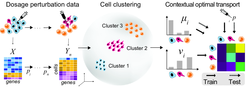
Figure 3: QontOT overview. A population of cells treated with varying drug dosages, resulting in ($X_{i},Y_{i},\bm{p}_{i}$) where $X_{i}$ ($Y_{i}$) represent scRNA-seq measurements before (after) a drug administered with dosage $\bm{p}_{i}\in[0,1]$. We cluster these measurements to identify cell types and then compute for each stage the distribution of cell types before and after perturbation, i.e., $\bm{\mu}$ and $\bm{\nu}$. A classical OT solver computes the ground truth OT plan $T_{i}$ based on $\bm{\mu}_{i}$, $\bm{\nu}_{i}$ (not shown). Given our initial cluster distribution before perturbation $\bm{\mu}_{i}$ and the dosage $\bm{p}_{i}$ our ansatz predicts a transportation plan $\bar{T}_{i}$.

We applied our method on predicting changes in the composition of a cell population due to drug perturbations and tested it on synthetic data and real data as visualized in Figure 3. Starting from a population of heterogeneous cells, each living in a high-dimensional state space we know that administering a drug has a direct effect on the composition of the cell population, by eliminating certain cell types or pushing some other cell types to proliferate. We denote as $\bm{\mu}$, $\bm{\nu}_{i}$ the cell type distribution of a cell population before and after the drug perturbation with a context variable $\bm{p}_{i}$, i.e., the drug dosage $\in[0,1]$. We measure performance on unseen dosages for different data splitting strategies.

4.1 Cell type assignment via clustering

We represent each cell through a single label, obtained through clustering from the original $\mathbb{R}^{l}$ space into $d$ clusters (i.e., cell types). We compute $\bm{\mu},\bm{\nu}\in\mathbb{R}^{d}$ as distributions over cluster labels for the population of cells before and after perturbation. In practice, we use $k$-Means clustering to cluster all cells of the training set and set $k=d$ to either $8$ or $16$ to adhere with the requirements of the quantum circuit, i.e., $d$ must be a power of $2$ (in general, if $\log_{2}{(k)}\not\in\mathbb{N}$, we pad and set $d:=2^{\left\lceil\log_{2}{(k)}\right\rceil}$ and fix the transportation plan to be diagonal for the padded entries). We then solve Equation 6 and compute the OT map between $\bm{\mu}$ and $\bm{\nu}$, using the entropically regularized Sinkhorn solver (Cuturi, 2013). Repeating this procedure for all dosages yields a dataset $\{T_{i},\bm{p}_{i}\}_{i=1}^{N}$ of transportation plan-perturbation tuples, processed as described in Section 3.3. The cost matrix $C\in\mathbb{R}^{d\times d}$ is the Euclidean or cosine distance between centroids.

5 Experimental results

This section verifies that QontOT (Quantum Contextual Optimal Transport) can learn to predict transportation maps contextualized through a perturbation variable.

5.1 Synthetic data

Leveraging the established sc-RNA-seq generator Splatter (Zappia et al., 2017), we devised a perturbation data generator that allows to control the number of generated cells, genes, cell types, perturbation functions and more. We experiment with different perturbation functions (that up-/downregulate gene expression linear or nonlinearly), different, distance metrics, number of clusters and data splits. Even though the perturbation functions are simple and only affect expression of a subset of cells and genes, the induced changes in cell type distribution are significant, locally continuous and nonlinear (cf. Figure A1). Details on the synthetic data generator and the used datasets are in Appendix A.1 and A.2.

We compare QontOT to two baselines, Average and Identity. Average always predicts the same transportation plan, obtained by solving the regularized OT problem (Equation 6) on all training samples at once, disregarding the context whereas Identity always predicts the identity OT plan, s.t., $\bm{\nu}=\bm{\mu}$. The results in Table 1 show that QontOT outperforms both baselines in all cases by a wide margin.

			OT Plan		Marginals
Dist.	Method	$\mathcal{L}$	SAE ($\downarrow$)	Frob. ($\downarrow$)	$L_{2}$ ($\downarrow$)	$R^{2}$ ($\uparrow$)
$L_{2}$	Identity	–	1.50	1.41	0.69	0.28
$L_{2}$	Average	–	1.07	0.79	0.52	0.27
$L_{2}$	QontOT	$\mathcal{L}_{T}$	0.97	0.70	0.45	0.56
$L_{2}$	QontOT	$\mathcal{L}_{M}$	0.97	0.79	0.41	0.55
Cos.	Identity	–	1.67	1.50	0.69	0.29
Cos.	Average	–	1.11	0.82	0.52	0.27
Cos.	QontOT	$\mathcal{L}_{T}$	0.97	0.71	0.44	0.59
Cos.	QontOT	$\mathcal{L}_{M}$	1.10	0.86	0.40	0.59

(a) Recovering effect of linear perturbation for different distances.

Dist.	Method	$\mathcal{L}$	SAE ($\downarrow$)	Frob. ($\downarrow$)	$L_{2}$ ($\downarrow$)	$R^{2}$ ($\uparrow$)
$L_{2}$	Identity	–	1.22	1.19	0.50	0.45
$L_{2}$	Average	–	0.97	0.72	0.41	0.42
$L_{2}$	QontOT	$\mathcal{L}_{T}$	0.86	0.62	0.34	0.47
$L_{2}$	QontOT	$\mathcal{L}_{M}$	0.97	0.77	0.32	0.48

(b) More realistic and challenging scenario of nonlinear perturbations.

Table 1: Transportation plan prediction. Performance in predicting transportation plans for unseen dosages and linear (a) and nonlinear (b) perturbations; comparing QontOT to two baselines. Different distance metrics were used to derive the cost matrix from the $K$-means centroids and both linear and non-linear perturbation effects were recovered. SAE denotes sum of absolute errors and Frobenius is the relative Frobenius norm. Means across three simulations are shown, full results in Table A1.

The two flavors of QontOT, $\mathcal{L}_{T}$ and $\mathcal{L}_{M}$ both have respective advantages; $\mathcal{L}_{T}$ models are explicitly trained on the transport plan. They provide solutions with lower cost but instead the $\mathcal{L}_{M}$ models only optimize the marginal distribution and give typically better results in $L_{2}$ and $R^{2}$. Unlike related work (Bunne et al., 2022), our method supports various costs like Euclidean or cosine distances of centroids, not just squared Euclidean. The exemplary real and predicted transportation plans in Figure 4A show that QontOT learns context-dependent shifts in cell type frequencies, by capturing the change in the distribution of cluster labels induced by the perturbation. Predicting the effect of stronger perturbations (higher dosages) is more challenging (cf. Figure 4B).

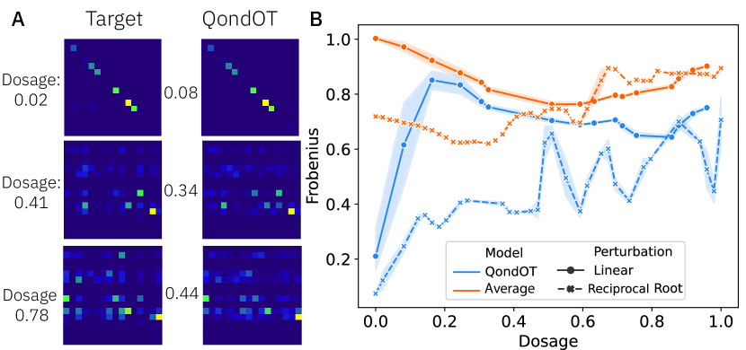
Figure 4: Capturing variation in cell type distributions. a) Three predicted transportation plans from the nonlinear perturbation dataset are shown next to their unseen ground truth. b) Frobenius distance of real and predicted transportation across unseen dosages are shown for QontOT and the baseline.

This is expected because in the control condition ($\bm{p}_{i}=0$), the cell type distribution remains identical, subject only to stochastic effects in data generation and batch assembly.

Circuit ablations.

Next we sought to assess the robustness of QontOT to different configurations: the choice of ansatz, the optimizer, the number of layers and auxilliary qubits and the aggregation scheme to obtain a right stochastic matrix. This time we used synthetic data with four cell groups (rather than one) that simulates more complex tissue and yields richer OT plans.

Method	SAE ($\downarrow$)	Frob. ($\downarrow$)	$L_{2}$ ($\downarrow$)	$R^{2}$ ($\uparrow$)
Identity	$0.65$	$0.60$	$0.18$	$0.46$
Average	$1.23$	$0.83$	$0.15$	$0.56$
$\mathcal{L}_{M}$	$0.59$	$0.43$	$0.13$	$0.58$
$\mathcal{L}_{T}$-Nevergrad	$0.41$	$0.30$	$0.14$	$0.54$
$\mathcal{L}_{T}$	$0.41$	$0.30$	$0.13$	$0.54$
$\mathcal{L}_{T}$-AsIs	$0.45$	$0.34$	$0.14$	$0.54$
$\mathcal{L}_{T}$-Simple	$0.46$	$0.32$	$0.13$	$0.57$
$\mathcal{L}_{T}$-Simple-12	$0.55$	$0.40$	$0.13$	$0.58$
$\mathcal{L}_{T}$-Simple-12-Shared	$0.41$	$0.30$	$0.14$	$0.57$
$\mathcal{L}_{T}$-Simple-16-Shared	$0.41$	$0.30$	$0.14$	$0.58$

Table 2: Ablation studies on circuit structure. $\mathcal{L}_{T}$ is the base configuration. Simple is an circuit constructions alternative to the base type "centrosymmetric" (cf. Appendix A.3 for details). "12" or "16" refers to the number of layers (base is $6$) and "Shared" defines whether the ansatz parameters are identical across layers (this is faster to optimize thus allowing deeper circuits). "AsIs" denotes an alternative to the "atop" aggregation to produce a DSM (cf. Section 3.2). Means across three random splits are shown.

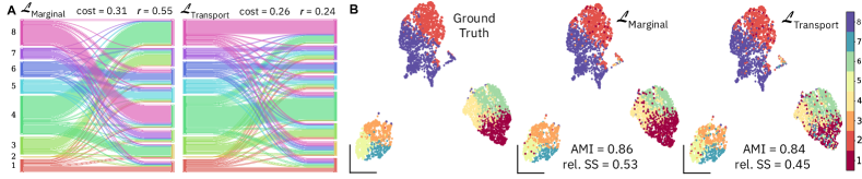
Figure 5: Comparison of QontOT optimization modes. A) Sankey plots of $\mathcal{L}_{Marginal}$ and $\mathcal{L}_{Transport}$ for a validation sample of pracinostat reveal that $\mathcal{L}_{M}$ learns transport maps with higher transport cost and unnecessary move of mass (see bucket $4$ and $8$). B) In contrast, the marginal performance of $\mathcal{L}_{M}$ is typically better, evidenced by the more discriminative cell type identification for the UMaps. The higher AMI (adjusted mutual information (Vinh et al., 2009)) shows that the predicted clusters are more similar to the real ones and the relative silhouette score (Rousseeuw, 1987) shows that the clusters are more consistent for $\mathcal{L}_{M}$ than for $\mathcal{L}_{T}$.

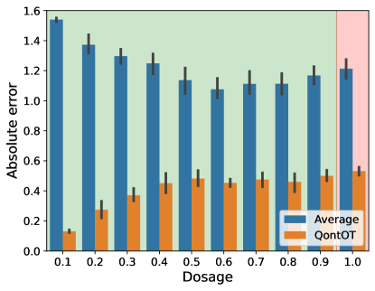
Figure A2: Out-of-distribution scenario. When QontOT is evaluated on dosages outside the training data scenario (redly shaded background), the performance decreases but still remains well above the baseline.

Overall, QontOT is robust to small alterations in circuit structure (cf. Table 2). Even though many of them use a slightly larger computational budget, none of the settings improve consistently across metrics over the base configuration, validating the imposed inductive biases, e.g., our ansatz type and the "atop" aggregation. Extending the number of layers in the ansatz or adding more auxilliar qubits also does not necessarily improve performance (more results in Table A2). Moreover, we find that in an OOD (out-of-distribution) setting where we kept the $10\%$ highest dosages out, the test error increases only mildly compared to the training error (cf. Figure A2).

Interestingly, the embedding for transportation maps with given initial distribution $\bm{\mu}$ proposed in Section 3.2 can be adapted to classical neural networks. The resulting quantum-inspired algorithm is described in Appendix C and performs explicit optimization of transport plans without relying on Brenier. Note, however, that it cannot be applied to the contextual (relaxed) assignment problem of predicting DSMs which we believe to be challenging for classical ML. While QontOT uses gradient-free optimization (with COBYLA or Nevergrad (Bennet et al., 2021)), the quantum-inspired approach can be trained conventionally with backpropagation and thus outperforms QontOT on the aforementioned datasets. We found that gradient-based, quasi-Newton optimization through BFGS substantially improves QontOT’s performance in simulation, however, it is currently not amenable to quantum hardware. Encouragingly even with gradient-free optimization there are cases where QontOT yields identical or slightly superior performance e.g., if the Hamiltonian of the system is known (cf. Table A3).

5.2 SciPlex data

To facilitate comparison with prior art, we compared QontOT to CellOT (Bunne et al., 2023) and CondOT (Bunne et al., 2022) on two drugs from the SciPlex dataset (Srivatsan et al., 2020) each administered in four dosages. For each of the dosages and the control condition, $20\%$ of cells were randomly held out for validation.

Method	SAE ($\downarrow$)	Frob. ($\downarrow$)	$L_{2}$ ($\downarrow$)	$R^{2}$ ($\uparrow$)
Identity	$1.10$	$1.04$	$0.18$	$0.47$
QontOT-$\mathcal{L}_{T}$	$0.78$	$0.61$	$0.17$	$0.49$
QontOT-$\mathcal{L}_{M}$	$0.92$	$0.68$	$0.16$	$0.57$
CellOT	$0.46$	$0.41$	$0.17$	$0.52$
CellOT-homo	$0.68$	$0.60$	$0.29$	$0.37$
CondOT	$0.45$	$0.40$	$0.18$	$0.56$

(a) Mocetinostat

Method	SAE ($\downarrow$)	Frob. ($\downarrow$)	$L_{2}$ ($\downarrow$)	$R^{2}$ ($\uparrow$)
Identity	$1.10$	$1.01$	$0.28$	$0.43$
QontOT-$\mathcal{L}_{T}$	$0.82$	$0.60$	$0.17$	$0.49$
QontOT-$\mathcal{L}_{M}$	$0.97$	$0.82$	$0.24$	$0.47$
CellOT	$0.44$	$0.40$	$0.18$	$0.56$
CellOT-homo	$0.93$	$0.80$	$0.45$	$0.27$
CondOT	$0.70$	$0.55$	$0.32$	$0.49$

(b) Pracinostat

Table 3: SciPlex comparison. Means across three runs are shown.

Table 3 indicates that CellOT largely yields the best results, note however, that it is an unconditional model and five models were trained (one per condition) inducing an unfair comparison. When aggregating data across conditions (CellOT-homo), performance drops below the level of QontOT-$\mathcal{L}_{T}$. This is a testimony of the competitiveness of our quantum approach. CondOT is an evolution of CellOT that leverages partial ICNNs (PICNNs) and can be parameterized by dosage. This yielded overall the best results on transportation plan metrics but on the marginal metrics $L_{2}$ and $R^{2}$, QontOT is on par or even superior. Notably, in many applications, such marginal metrics are of higher importance. They can be directly optimized in QontOT’s $\mathcal{L}_{M}$ optimization mode which depicts a form of weakly supervised amortized optimization of transport plans that also overcomes the dependence on conventional OT solvers to compute training samples (cf. Section 2.3). The duality of QontOT’s optimization mode is visualized and explained in Figure 5.

6 Discussion

In this work we have introduced a principled approach to represent transportation maps on quantum computers. We proposed an ansatz for learning to predict OT maps conditioned on a context variable, without requiring access to the cost matrix. Our empirical results evidence that our method can successfully learn to predict contextualized transportation maps. Exemplified on synthetic and real data of single-cell drug dosage perturbations, our method is able to predict transportation plans representing distributional shifts in cell type assignments. While our method does not exceed performance of the best classical models, it constitutes, to the best of our knowledge, the first approach to bridge OT and ML on quantum computers. Notably our approach does not impose general constraints on the dimensionality of the context variable(s), thus more complex perturbations such as continuous drug representations, combinatorial genetic perturbations or other covariates could be also employed. Given that, in our described application, the dosage-induced shifts in cluster assignments are also largely driven by the initial cell states (rather than only the dosage), future work will be devoted to make our ansatz fully parametric for $\bm{\mu}_{i}$, potentially through (unbalanced) co-optimal transport (Titouan et al., 2020; Tran et al., 2023).

Impact statement

This paper presents work with the goal to advance the field of quantum machine learning (QML). There are many potential societal consequences of advances in quantum computing, first and foremost in cryptanalysis (see Scholten et al. (2024) for a broad overview). Next, advances in QML will have more specific implications, e.g., they could widen disparities between organizations, countries or researchers that have access to, or can afford, leveraging quantum computing and those that cannot. However, beyond these general consequences, we can not weave any implications specific to our work.

Appendix

Appendix A Experimental details

A.1 Synthetic dosage perturbation data generator

We leverage the established single-cell RNA sequencing generator Splatter (Zappia et al., 2017) to form a three-stage generator for drug dosage perturbation datasets:

1. First, Splatter samples raw expression counts ($X\in\mathbb{R}^{n_{1}\times l}$, with $n_{1}$ cells and $l$ genes) from zero-inflated negative binomial distributions (one per gene). Sufficient statistics of all underlying distributions (Poisson, Gamma, Chi-Square) can be controlled.

2. We aim to produce a tuple of ($X_{i},Y_{i},\bm{p}_{i}$) where $X_{i}$ holds unperturbed base states of $n_{1}$ cells and $Y_{i}\in\mathbb{R}^{n_{2}\times l}$ holds perturbed states of $n_{2}$ cells, resulting from a drug perturbation administered with dosage $\bm{p}_{i}\in[0,1]$. To derive the perturbed states $Y_{i}$, new base states $\bar{Y}_{i}$ are sampled with the same configuration used to generate $X_{i}$, mimicking that cells are being destroyed during measurement. Subsequently $Y_{i}=g(\bar{Y}_{i},\bm{p}_{i})$ where $g$ is the total effect on the cells, governed by a combination of noise terms and the immediate effect $g_{p}(\cdot)$ of the perturbation. We assume that only $15\%$ of the genes alter their expression upon perturbation. In this case, we apply $g_{p}$ to the raw cell states, scaled by a response amplitude $\sim\mathcal{U}(0.3,1)$. Moreover, $10\%$ of the cells are generally unresponsive to the perturbation ($g_{p}=0$). We investigate linear and non-linear perturbations, i.e., $g_{p_{1}}(x)=ax+b$ and a reciprocal root function $g_{p_{2}}(x)=ax^{-b}$ with $a,b>0$, respectively. The hyperparameters of the experiments can be found in Appendix A.2.

3. We repeat stage 2 for each dosage by varying smoothly the immediate effect $g_{p}(\cdot)$ based on $\bm{p}_{i}$, resulting in a dataset $\{X_{i},Y_{i},\bm{p}_{i}\}_{i=1}^{N}$ of $N$ tuples. Responsive genes are fixed across samples. The base states $X_{i}$ are identical across all samples of the dataset, mimicking the common experimental setting where only one control population was measured (Srivatsan et al., 2020).

Figure A1: Exemplary cell type distributions for source and target cell populations. The distribution of cell types in the unperturbed tissue is either entirely static (see left) or varies mildly based on the user-defined noise level (not shown). Instead, the perturbed cells produce highly dissimilar distributions that, however, exhibit some local continuity for similar dosages. The plot was generated with data from linear perturbations and euclidean cost.

A.2 Datasets and hyperparameters

A.2.1 Synthetic data

Initial experiments

For the results shown in Table 1 and Figure 4, we simulate 300 genes and 1000 cells across 50 unique dosages, equidistantly spaced in $[0,1]$. 15% of the genes respond to the perturbation $g_{p}(\cdot)$ but $10\%$ of the cells are set as unresponsive. The sinkhorn regularization $\gamma=0.001$. For the linear case, $f_{p_{1}}(x)=3x+1$ and for the non-linear case $f_{p_{2}}(x)=100x^{-0.2}$. For each dosage, four batches of $500$ cells each were created, summing to 200 samples which were split randomly with $20\%$ held out dosages for testing. In almost all experiments we set the number of clusters to $k=d=8$; only in Figure 4 it was set to $16$.

Four cell groups.

For the ablation studies on circuit structure and extrapolation (cf. Table 2), we simulate populations of $100$ genes and $2000$ cells, each belonging now to one out of four groups to simulate more complex tissue. We perturb the populations with the function $f_{p_{2}}$ (as above) and $100$ dosages, equidistantly spaced in $[0,1]$. The initial cell states $X_{i}$ are resampled for every dosage and only $2\%$ of cells are set as unresponsive. The $100$ dosages are split randomly with $20\%$ test data.

A.2.2 SciPlex data

Selected models were trained on two of the nine compounds from the SciPlex dataset (Srivatsan et al., 2020). High Throughput Screens on three cell lines were conducted with four varying concentrations (10, 100, 1000, and 10000 nM) for each drug. We inherit preprocessing from Bunne et al. (2023) and Lotfollahi et al. (2019) which includes library size normalization, filtering at the cell and gene levels, and log1p transformation. For mocetinostat and pracinostat we obtained respectively 22,154 and 21,926 cells from which 17,565 and 15,137 were control cells. Data was split per condition (control + four dosages) in a roughly 80/20 ratio. Preprocessing identified 1,000 highly-variable genes, which were fed through scGen (Lotfollahi et al., 2019) to obtain 50-dimensional latent codes, just like in prior art (Bunne et al., 2022, 2023; Uscidda & Cuturi, 2023). The latent codes are clustered with $K$-Means into $8$ clusters.

CellOT & CondOT.

CellOT and CondOT are trained with the ott-jax package (Cuturi et al., 2022) for $1000$ iterations and batches of size $50$ on $\bm{\mu}_{i}$, i.e., the same $8$-dimensional feature vectors (denoting a distribution of cell types over $50$ cells) used to train QontOT. We use a cosine decay learning rate scheduler with an initial value of $0.001$ and an alpha of $0.01$, optimized with ADAM (Kingma & Ba, 2014). CondOT uses the gaussian map initialization proposed in (Bunne et al., 2022). As CellOT and CondOT learn directly a map $f:\mathbb{R}^{8}\rightarrow\mathbb{R}^{8}$ such that $f(\bm{\mu}_{i})=\bar{\bm{\nu}_{i}}$, we use the entropically regularized sinkhorn solver (Cuturi, 2013) on $(\bm{\mu}_{i},\bm{\nu}_{i})$ to obtain the transport maps and compute performance metrics on SAE and relative Frobenius norm.

A.3 Implementation

As mentioned in Section 3, the fact that $U\odot\overline{U}\in\Omega_{n}$ is a DSM offers great flexibility in the choice of the ansatz. In practice, we implemented two ansätze, centrosymmetric and simple. Both of them have been implemented and trained in Qiskit 0.43.0 (Qiskit contributors, 2023) and all experiments were performed with Qiskit’s sampler class in state vector simulation.

Centrosymmetric

The centrosymmetric ansatz is our default implementation which induces a bias toward properties of centrosymmetric matrices. Specifically, the matrix being modelled can be divided into four quadrants such that the respective diagonals are equal and the respective off-diagonals are also equal.

Simple

Instead, the simple ansatz instead is symmetric by construction and has less bias toward a specific class of unitary operators than the centrosymmetric ansatz. This ansatz was first formulated in Khatri et al. (2019) and later refined in Madden & Simonetto (2022). Note that this ansatz implements the identity operator when all parameters are zero.

Appendix B Extended Results

				Transportation plan		Marginals
Perturb.	Dist.	Layers	$\mathcal{L}$	SAE ($\downarrow$)	Frob. ($\downarrow$)	$L_{2}$ ($\downarrow$)	$R^{2}$ ($\uparrow$)
Lin.	$L_{2}$	Ident.	–	$1.50_{\pm 0.14}$	$1.41_{\pm 0.12}$	$0.69_{\pm 0.07}$	$0.28_{\pm 0.07}$
Lin.	$L_{2}$	Avg.	–	$1.07_{\pm 0.04}$	$0.79_{\pm 0.01}$	$0.52_{\pm 0.04}$	$0.27_{\pm 0.06}$
Lin.	$L_{2}$	QontOT	$\mathcal{L}_{T}$	$0.97_{\pm 0.08}$	$0.70_{\pm 0.06}$	$0.45_{\pm 0.04}$	$0.56_{\pm 0.03}$
Lin.	$L_{2}$	QontOT	$\mathcal{L}_{M}$	$0.97_{\pm 0.12}$	$0.79_{\pm 0.15}$	$0.41_{\pm 0.05}$	$0.55_{\pm 0.10}$
Lin.	Cos.	Ident.	–	$1.67_{\pm 0.16}$	$1.50_{\pm 0.13}$	$0.69_{\pm 0.07}$	$0.29_{\pm 0.07}$
Lin.	Cos.	Avg.	–	$1.11_{\pm 0.05}$	$0.82_{\pm 0.02}$	$0.52_{\pm 0.05}$	$0.27_{\pm 0.06}$
Lin.	Cos.	QontOT	$\mathcal{L}_{T}$	$0.97_{\pm 0.09}$	$0.71_{\pm 0.07}$	$0.44_{\pm 0.05}$	$0.59_{\pm 0.02}$
Lin.	Cos.	QontOT	$\mathcal{L}_{M}$	$1.10_{\pm 0.14}$	$0.86_{\pm 0.10}$	$0.40_{\pm 0.06}$	$0.59_{\pm 0.10}$
NonLin.	$L_{2}$	Ident.	–	$1.22_{\pm 0.05}$	$1.19_{\pm 0.05}$	$0.50_{\pm 0.02}$	$0.45_{\pm 0.02}$
NonLin.	$L_{2}$	Avg.	–	$0.97_{\pm 0.02}$	$0.72_{\pm 0.01}$	$0.41_{\pm 0.01}$	$0.42_{\pm 0.04}$
NonLin.	$L_{2}$	QontOT	$\mathcal{L}_{T}$	$0.86_{\pm 0.03}$	$0.62_{\pm 0.02}$	$0.34_{\pm 0.01}$	$0.47_{\pm 0.05}$
NonLin.	$L_{2}$	QontOT	$\mathcal{L}_{M}$	$0.97_{\pm 0.06}$	$0.77_{\pm 0.05}$	$0.32_{\pm 0.01}$	$0.48_{\pm 0.01}$

Table A1: Transportation plan prediction. Extended results for Table 1, $\pm$ denotes standard deviation across three runs.

Dist.	Layers	$\mathcal{L}$	SAE ($\downarrow$)	Frob. ($\downarrow$)	$L_{2}$ ($\downarrow$)	$R^{2}$ ($\uparrow$)
$L_{2}$	6	$\mathcal{L}_{T}$	$0.97_{\pm 0.08}$	$0.70_{\pm 0.06}$	$0.45_{\pm 0.04}$	$0.56_{\pm 0.03}$
$L_{2}$	12	$\mathcal{L}_{T}$	$0.98_{\pm 0.11}$	$0.72_{\pm 0.08}$	$0.45_{\pm 0.05}$	$0.53_{\pm 0.10}$
$L_{2}$	6	$\mathcal{L}_{M}$	$0.97_{\pm 0.12}$	$0.79_{\pm 0.15}$	$0.41_{\pm 0.05}$	$0.55_{\pm 0.10}$
$L_{2}$	12	$\mathcal{L}_{M}$	$1.02_{\pm 0.09}$	$0.81_{\pm 0.13}$	$0.42_{\pm 0.04}$	$0.54_{\pm 0.08}$
Cos.	6	$\mathcal{L}_{T}$	$0.97_{\pm 0.09}$	$0.71_{\pm 0.07}$	$0.44_{\pm 0.05}$	$0.59_{\pm 0.02}$
Cos.	12	$\mathcal{L}_{T}$	$0.99_{\pm 0.10}$	$0.71_{\pm 0.06}$	$0.45_{\pm 0.05}$	$0.59_{\pm 0.17}$
Cos.	6	$\mathcal{L}_{M}$	$1.10_{\pm 0.14}$	$0.86_{\pm 0.10}$	$0.40_{\pm 0.06}$	$0.59_{\pm 0.10}$
Cos.	12	$\mathcal{L}_{M}$	$1.06_{\pm 0.05}$	$0.83_{\pm 0.12}$	$0.42_{\pm 0.05}$	$0.60_{\pm 0.12}$

Table A2: Ablation study on number of layers in ansatz. Adding more layers in the ansatz and thus more parameters in the circuit does not improve performance. Experiment performed on linear perturbation function (cf. Table 1). For $6$ respectively $12$ layers in the ansatz, there are $234$ respectively $456$ circuit parameters to optimize.

Appendix C Neural contextual OT (NeuCOT)

C.1 Methodology

In Section 3.2 we have shown that, if we produce a right stochastic matrix $\widehat{T}\in\mathcal{N}\left(\mathbf{1}_{d},\bm{\nu}^{\prime}\right)$, the latter can be rescaled to a transportation map with the required initial distribution $\bm{\mu}$. We recall that, at inference time, the right stochastic $\widehat{T}$ is predicted by a circuit depending on the perturbation, thus the predicted transportation map results from the rescaling of the rows of $\widehat{T}$, using the elements of the initial distribution $\bm{\mu}$ as coefficients. A complementary case is that of the contextual (relaxed) assignment problem, whose origin is presented in Section 2.2. The latter requires the prediction of a DSM, and we believe that this task is hard for classical machine learning. The former case instead, that is the one requiring a right stochastic matrix, can be shown to be practical for classical ML. Let $M\in\mathbb{R}^{d\times d}$ and $\left[e^{M_{i,j}}\right]$ the Hadamard exponential matrix (Horn & Johnson, 2012) of $M$, that is the matrix resulting from the entry-wise application of the exponential mapping. We extend the notation to a row-rescaled form, so

$$M\mapsto \left[\frac{e^{M_{i,j}}}{\sum_{k}e^{M_{i,k}}}\right],$$ (15)

then

$$\left[\frac{e^{M_{i,j}}}{\sum_{k}e^{M_{i,k}}}\right]\mathbf{1}_{d}=\begin{pmatrix}\frac{\sum_{k}e^{M_{1,k}}}{\sum_{k}e^{M_{1,k}}}&\cdots&\frac{\sum_{k}e^{M_{d,k}}}{\sum_{k}e^{M_{d,k}}}\end{pmatrix}^{\top}=\mathbf{1}_{d},$$ (16)

that is (15) maps any $M\in\mathbb{R}^{d\times d}$ to a right stochastic matrix. Let the matrix-valued function $f_{\bm{\theta}}:\mathcal{X}\to\mathbb{R}^{d\times d}$ represent a neural network parametrised by the vector $\bm{\theta}$, mapping the space of perturbations $\mathcal{X}$ to a $d\times d$ real matrix. We obtain a right stochastic matrix as a function of the perturbation $\mathbf{p}\in\mathcal{X}$, so

$$\widehat{T}= \left[\frac{e^{\left(f_{\bm{\theta}}(\mathbf{p})\right)_{i,j}}}{\sum_{k}e^{{\left(f_{\bm{\theta}}(\mathbf{p})\right)_{i,k}}}}\right]\in\mathcal{N}\left(\mathbf{1}_{d},\bm{\nu}^{\prime}\right).$$ (17)

Hence, the right stochastic matrix can be obtained through a neural network with a softmax activation in the ultimate layer. Finally the procedure continues as outlined in Section 3.2, that is the prediction for the transportation map is given by $\bar{T}=D_{\bm{\mu}}\widehat{T}$, so $\bar{T}\mathbf{1}_{d}=\bm{\mu}$ as required. Optionally, one can make the prediction depending non-linearly on the initial distribution $\bm{\mu}$ by re-defining $f_{\bm{\theta}}$ as a function of both the perturbation and the distribution $\bm{\mu}$.

This is a novel, quantum-inspired approach that combines neural and contextual OT through amortized optimization. It can be trained in a fully or weakly supervised setting, either optimizing OT plans directly (i.e., $\mathcal{L}(\bar{T},T)$) or only the push-forwarded distribution (i.e., $\mathcal{L}(\hat{T}\sharp\bm{\mu},\bm{\nu})$). We dub this approach NeuCOT for Neural Contextual Optimal Transport. Previous approaches either leverage Brenier’s theorem (1987) to recast the problem to convex regression (e.g., CellOT and CondOT (Bunne et al., 2022, 2023)) or use regularization (Uscidda & Cuturi, 2023). In the implementation the optimization occurs over the push-forwarded measure in both cases, so unlike in our method, the OT plans can not be directly accessed.

C.2 Implementation and Result

In practice, we implement this approach with a shallow, dense neural network ($64$ and $128$ units), a ReLU activation, a dropout of $40\%$ and use a MSE loss between real and predicted OT plans. The models have $\sim 17$k trainable parameters that are optimized with ADAM for $500$ epochs with a learning rate of $5\mathrm{e}{-4}$.

The results in Table A3 compare NeuCOT to QontOT and the average baseline for different datasets and splitting strategies.

Dataset	Data split	Method	SAE ($\downarrow$)	Frob. ($\downarrow$)	$L_{2}$ ($\downarrow$)	$R^{2}$ ($\uparrow$)
Four cell types	Random	Average	$1.23$	$0.83$	$0.15$	$0.56$
		QontOT	$0.41$	$0.30$	$0.13$	$0.54$
		NeuCOT	$0.22$	$0.20$	$0.10$	$0.73$
Four cell types	Extrapolation	Average	$1.21$	$0.84$	$0.24$	$0.09$
		QontOT	$0.53$	$0.78$	$0.20$	$0.21$
		NeuCOT	$0.32$	$0.30$	$0.17$	$0.39$
Known Hamiltonian $8\times 8$ plans	Random	Average	$2.332$	$0.883$	$0.538$	$0.880$
		QontOT-$\mathcal{L}_{T}$	0.571	0.208	0.085	$0.892$
		NeuCOT	$0.581$	$0.215$	$0.089$	0.894
Known Hamiltonian $16\times 16$ plans	Random	Average	$1.317$	$0.879$	$0.055$	$0.671$
		Identity	$0.878$	$1.042$	$0.078$	$0.640$
		QontOT-$\mathcal{L}_{T}$	$0.421$	$0.833$	$0.028$	0.710
		QontOT-$\mathcal{L}_{M}$	$0.479$	$0.845$	$0.029$	$0.699$
		NeuCOT	0.400	0.356	$0.028$	$0.708$

Table A3: Comparison of QontOT to NeuCOT. Means across three different runs are shown. All datasets use actual distributions, so $\bm{\mu}\mathbf{1}_{n}=1=\bm{\nu}\mathbf{1}_{n}$.

Appendix D Quantum formulation

D.1 Recovery of finitely-sampled matrices

In Section 3.1 we obtained a DSM from a quantum circuit by considering the measurements asymptotically. The objective of the present section is that of obtaining a method for estimating the DSM from finite measurements. We define a multiset as the tuple $\langle X,c_{X}\rangle$, where $X$ denotes the underlying set of elements and $c_{X}$ a function mapping each element $x\in X$ to its cardinality. Given the density matrix $\rho$ prepared as in (9a), we run a sampling process which produces a (nonempty) multiset $S=\langle\{(i,j)\},c\rangle$ of pairs $\{(i,j)|i,j\in\left[0\mathinner{\ldotp\ldotp}{}d-1\right]\}$, where $i$ and $j$ correspond respectively to the row and column indices of the DSM being sampled. The pairs $(i,j)$ are counted using a (non-negative) $d\times d$ matrix $F$ whose entries $F_{i,j}$ correspond to the relative frequency of each pair, that is

$$F_{i,j}= \frac{c(\,(i,j)\,)}{\sum_{i^{\prime},j^{\prime}}c(\,(i^{\prime},j^{\prime})\,)}.$$ (18)

By previous the definition we note that $\mathbf{1}_{d}^{\top}F\mathbf{1}_{d}=1$ (i.e. $F$ has total mass $1$), and asymptotically the matrix $dF$ (i.e. rescaled to have total mass $d$) approaches the DSM in (10b). Assuming the matrix $F$ is non-zero (that is we acquired at least one sample), we define the projector onto the Birkhoff polytope as

$$Q^{\star}= \underset{Q\in\Omega_{d}}{\mathrm{argmin}}\left\|Q-dF\right\|^{2}_{F}.$$ (19)

Then, by the closedness and convexity of $\Omega_{d}$ the solution $Q^{\star}$ always exists and is unique. We note that when $dF\in\Omega_{d}$, that is the input matrix is already DSM, then the minimizer becomes $Q^{\star}=dF$. In other words, the projection acts as the identity operator when the input matrix belongs to the Birkhoff polytope.

The remaining part of this section is going to focus on estimating the sampling error for the case of right stochastic matrices (see Section 3.2) obtained from the matrix of relative frequencies $F$. To solve the problem, we employ the Kullback-Leibler (KL) divergence to quantify the informational difference between probability distributions. We minimize the KL divergence, so

$$\underset{Q\in\mathbb{R}^{d\times d}_{+}}{\min}\, \sum\limits_{i,j=1}^{n}Q_{i,j}\ln\left(\frac{Q_{i,j}}{dF_{i,j}}\right),$$ (20a)

s.t. $$Q\mathbf{1}_{d}=\mathbf{1}_{d}.$$ (20b)

Leveraging Lagrange multipliers, denoted as $a_{i}$, the objective function becomes

$$\mathcal{L}(Q) =\sum\limits_{i,j=1}^{d}\left(Q_{i,j}\ln\left(\frac{Q_{i,j}}{dF_{i,j}}\right)+a_{i}(Q_{i,j}-1)\right),$$ (21)

$$\frac{\partial\mathcal{L}}{\partial Q_{i,j}} =\ln Q_{i,j}-\ln(dF_{i,j})+1+a_{i}=0\implies Q=d\cdot\mathrm{diag}(\widetilde{\mathbf{a}})F,$$

with $\widetilde{\mathbf{a}}\in\mathbb{R}_{++}^{d}$. By imposing the constraint $Q\mathbf{1}_{d}=\mathbf{1}_{d}$ and assuming that $F\mathbf{1}_{d}\in\mathbb{R}_{++}^{d}$, it follows that $\mathrm{diag}(\widetilde{\mathbf{a}})=\frac{1}{d}\mathrm{diag}(F\mathbf{1})^{-1}$, hence we obtain the minimizer

$$Q^{\star} =d\cdot\mathrm{diag}(\widetilde{\mathbf{a}})F=\mathrm{diag}(F\mathbf{1})^{-1}F.$$ (22)

To obtain the latter we have assumed that $F\mathbf{1}_{d}\in\mathbb{R}_{++}^{d}$, that is the row vectors of $F$ are non-zero. To prevent this scenario, it is essential to determine the minimum number of shots required. This count can be derived from the "Coupon Collector’s Problem." (Blom et al., 1994). It indicates that to achieve a satisfactory probability (of obtaining $F$ with nonzero rows) $p$, we need at least

$$N_{0}=d\ln\left(\frac{d}{1-p}\right)$$ (23)

samples, and $1-p\ll 1$.

We remark that the minimum number of samples $N_{0}$, relates to the requirement regarding the non-zero rows in the matrix $F$. However, the latter does not cover the minimum number of shots to obtain a given precision $\varepsilon$ for each entry of the resulting matrix. Indeed, for each entry of the matrix $Q^{\star}$ we need $\mathcal{O}(1/\varepsilon^{2})$ measurements to obtain precision $\varepsilon$, consequently we require $\mathcal{O}(d^{2}/\varepsilon^{2})$ measurements for the entire matrix.

D.2 The checkerboard ansatz

We propose an ansatz construction which is convenient with respect to the structure of the embedding of transportation maps expanded in Section 3.2. Specifically, since in the partitioning of the DSM in (11), only the top two quadrants contribute to the resulting right stochastic matrix, we aim at devising an ansatz that does not carry additional information in the discarded quadrants. The latter could also be interpreted as making the parametrisation for the ansatz more efficient.

For some positive integer $k$, we define the subset $G_{k}$ of unitary operators as

$$G_{k}\coloneqq \left\{U\in\mathsf{U}\left({2k}\right)\,\middle\rvert\,U=\mathbb{I}_{2}\otimes A+\sigma_{x}\otimes B\right\},$$ (24)

where $A,B$ are $k\times k$ matrices, not necessarily unitary. In other words, the operators in $U\in G_{k}$ have the following block matrix form

$$U= \begin{pmatrix}A&B\\ B&A\end{pmatrix},$$ (25)

which is clearly inherited by the corresponding unistochastic

$$U\odot\overline{U}= \begin{pmatrix}A\odot\overline{A}&B\odot\overline{B}\\ B\odot\overline{B}&A\odot\overline{A}\end{pmatrix}=\begin{pmatrix}Q_{1}&Q_{2}\\ Q_{2}&Q_{1}\end{pmatrix}.$$ (26)

We now proceed with revealing the group-theoretical structure of the set $G_{k}$ and also its relation with the tensor product, hence we obtain the construction of the ansatz implementing the unitary in (25).

The next lemma shows that the set $G_{k}$ is a subgroup of even degree of the unitary group.

Lemma D.1.

The set $G_{k}$ is non-empty and endowed with a group structure under operator composition, for all positive integers $k$.

Proof.

It is immediately verifiable that $\mathbb{I}_{2k}\in G_{k}$, that is the set $G_{k}$ is non-empty and it contains the identity element w.r.t. matrix multiplication. Also the composition of operators carries the associativity as required. Finally we verify the closure. Let $U_{1},U_{2}\in G_{k}$ such that $U_{i}=\mathbb{I}_{2}\otimes A_{i}+\sigma_{x}\otimes B_{i}$ for $i=1,2$, then

$$U_{1}U_{2}= \left(\mathbb{I}_{2}\otimes A_{1}+\sigma_{x}\otimes B_{1}\right)\left(\mathbb{I}_{2}\otimes A_{2}+\sigma_{x}\otimes B_{2}\right)$$ (27a)

$$= \mathbb{I}_{2}\otimes\left(A_{1}A_{2}+B_{1}B_{2}\right)+\sigma_{x}\otimes\left(A_{1}B_{2}+B_{1}A_{2}\right),$$ (27b)

which corresponds to the pattern in (25). Hence $U_{1}U_{2}\in G_{k}$. ∎

The result that follows shows that the structure is preserved under the tensor product.

Lemma D.2.

Let $U_{1}\in G_{k_{1}}$ and $U_{2}\in G_{k_{2}}$, for some positive integers $k_{1}$ and $k_{2}$. Then $U_{1}\otimes U_{2}\in G_{2k_{1}k_{2}}$.

Proof.

Let $U_{1}\in G_{k_{1}}$ and $U_{2}\in G_{k_{2}}$ such that $U_{i}=\mathbb{I}_{2}\otimes A_{i}+\sigma_{x}\otimes B_{i}$ for $i=1,2$, then

$$U_{1}\otimes U_{2}= \left(\mathbb{I}_{2}\otimes A_{1}+\sigma_{x}\otimes B_{1}\right)\otimes\left(\mathbb{I}_{2}\otimes A_{2}+\sigma_{x}\otimes B_{2}\right)$$ (28a)

$$= \mathbb{I}_{2}\otimes A+\sigma_{x}\otimes B,$$ (28b)

with $A=A_{1}\otimes\left(\mathbb{I}_{2}\otimes A_{2}+\sigma_{x}\otimes B_{2}\right)$ and $B=B_{1}\otimes\left(\mathbb{I}_{2}\otimes A_{2}+\sigma_{x}\otimes B_{2}\right)$. Hence it follows that $U_{1}\otimes U_{2}$ fulfils the pattern in (25) and since $A,B$ are linear maps in $\mathbb{C}^{2k_{1}k_{2}}$, then $U_{1}\otimes U_{2}\in G_{2k_{1}k_{2}}$. ∎

D.2.1 Ansatz’s two-qubit generator

We obtain a two-qubit circuit $U_{g}\in G_{2}$, that by Lemma D.1 and D.2 can be used as a generator for the more general $G_{2^{k}}$ with $k\geq 1$. From the definition in (24) we obtain the symmetry $U\in G_{2}\implies(\sigma_{x}\otimes\mathbb{I}_{2})U(\sigma_{x}\otimes\mathbb{I}_{2})=U$. Using the latter and the general unitary circuit with 2 CNOTs (highlighted) (Barenco et al., 1995), we solve the following circuit equation

$$\vbox{ \Qcircuit@C=0.5em @R=0.25em @!R { \nghost{ {q}_{0} } & \lstick{ {q}_{0} } \qw \gate{C} \targ \gate{R_z(\alpha)} \targ \gate{A} \qw \qw \qw \gate{A^\dagger} \targ \gate{R_z(-\alpha)} \targ \gate{C^\dagger} \qw \qw \qw\\ \nghost{ {q}_{1} } \lstick{ {q}_{1} } \qw \gate{D} \ctrl{-1} \gate{R_y(\beta)} \ctrl{-1} \gate{B} \qw \gate{X} \qw \gate{B^\dagger} \ctrl{-1} \gate{R_y(-\beta)} \ctrl{-1} \gate{D^\dagger} \qw \gate{X} \qw\gategroup{1}{4}{2}{8}{.7em}{--} }}=\mathbb{I}_{2}^{\otimes 2},$$ (29)

where $A,B,C,D$ are arbitrary single qubit (special) unitaries and $\alpha,\beta\in\mathbb{R}$. We obtain a solution to the equation. Since the operator $\sigma_{z}\otimes\mathbb{I}_{2}$ commutes with the CNOT gate (with the Pauli $\sigma_{z}$ acting on CNOT’s controlling qubit), we impose on (29) the conditions

$$B^{\dagger}\sigma_{x}B= \sigma_{z},$$ (30a)

$$R_{y}(-\beta)\sigma_{z}R_{y}(\beta)= \sigma_{z},$$ (30b)

$$D^{\dagger}\sigma_{z}D= \sigma_{x}.$$ (30c)

Then a solution is $B=D=H$ and $\beta=0$, where $H$ is the Hadamard operator on a single qubit. Hence the generator circuit takes the following form

$$\Qcircuit@C=0.5em@R=0.25em@!R{\nghost{{q}_{0}}&\lstick{{q}_{0}}\qw\gate{C}\targ\gate{R_{z}(\alpha)}\targ\gate{A}\qw\\ \nghost{{q}_{1}}\lstick{{q}_{1}}\qw\gate{H}\ctrl{-1}\qw\ctrl{-1}\gate{H}\qw}$$ (31)

where $A,C\in SU(2)$ and $\alpha\in\mathbb{R}$.

Finally, by using Lemma D.1 and D.2, and the generator block in (31), we construct the ansatz as exemplified in Figure A3.

$$\Qcircuit@C=0.5em@R=0.50em@!R{\nghost{{q}_{1}:\ket{0}}&\lstick{{q}_{1}:}\multigate{1}{\mathrm{K}(\bm{\theta}_{1})}\qw\qw\qw\\ \nghost{{q}_{2}:\ket{0}}\lstick{{q}_{2}:}\ghost{\mathrm{K}(\bm{\theta}_{1})}\qw\multigate{1}{\mathrm{K}(\bm{\theta}_{3})}\qw\\ \nghost{{q}_{3}:\ket{0}}\lstick{{q}_{3}:}\multigate{1}{\mathrm{K}(\bm{\theta}_{2})}\qw\ghost{\mathrm{K}(\bm{\theta}_{3})}\qw\\ \nghost{{q}_{4}:\ket{0}}\lstick{{q}_{4}:}\ghost{\mathrm{K}(\bm{\theta}_{2})}\qw\multigate{1}{\mathrm{K}(\bm{\theta}_{4})}\qw\\ \nghost{{q}_{5}:\ket{0}}\lstick{{q}_{5}:}\qw\qw\ghost{\mathrm{K}(\bm{\theta}_{4})}\qw}$$

Figure A3: An example of depth and connectivity efficient (single) layer for the Checkerboard ansatz. Here the blocks $K$ correspond to the 2-qubits circuit in (31) and the vectors $\bm{\theta}_{i}$ are seven dimensional vectors parameterizing gates $A,C$ and $\mathrm{R}_{z}$ of (31).

D.3 Proofs

Proof of Lemma 2.1.

Considering the constraint $\operatorname{Tr}\left(U_{i}U_{j}^{\dagger}\right)=n\delta_{ij}$ we obtain

$$\operatorname{\mathrm{vec}_{r}}(U_{j})^{\dagger}\operatorname{\mathrm{vec}_{r}}(U_{i})= \sum_{k}\left(\bra{k}U_{j}^{\dagger}\otimes\bra{k}\right)\sum_{t}\left(U_{i}\ket{t}\otimes\ket{t}\right)$$ (32a)

$$= \sum_{k,t}\left(\bra{k}U_{j}^{\dagger}U_{i}\ket{t}\otimes\bra{k}\ket{t}\right)$$ (32b)

$$= \sum_{k}\left(\bra{k}U_{j}^{\dagger}U_{i}\ket{k}\right)=\operatorname{Tr}\left(U_{i}U_{j}^{\dagger}\right)=n\delta_{ij}.$$ (32c)

∎

Proof of Lemma 3.1.

We expand the function $p:\left[0\mathinner{\ldotp\ldotp}{}d-1\right]\times\left[0\mathinner{\ldotp\ldotp}{}d-1\right]\to[0,1]$ defined in (10a), so

$$p(i,j)\coloneqq 2^{n}\operatorname{Tr}(\rho\ket{ij}\bra{ij})$$ (33a)

$$= \sum_{k}\lambda_{k}^{2}\bra{ij}\operatorname{\mathrm{vec}_{r}}\left(W_{k}\right)\operatorname{\mathrm{vec}_{r}}\left(W_{k}\right)^{\dagger}\ket{ij}$$ (33b)

$$= \sum_{k}\lambda_{k}^{2}\bra{i}\left(W_{k}\odot\overline{W_{k}}\right)\ket{j}.$$ (33c)

The positivity of the entries of the DSM is clear from the definition of $p(i,j)$. We prove the rows sum constraint for $Q=\sum_{i,j}p(i,j)\ket{i}\bra{j}$, that is

$$Q\mathbf{1}_{d}= \sum_{i,j}p(i,j)\ket{i}$$ (34a)

$$= \sum_{i}\ket{i}\cdot\left(\sum_{k}\lambda_{k}^{2}\bra{i}\sum_{j}\left(W_{k}\odot\overline{W_{k}}\right)\ket{j}\right),$$ (34b)

where the rightmost sum equals the vector $\mathbf{1}_{m}$ since $W_{k}\odot\overline{W_{k}}$ is unistochastic, also $\sum_{k}\lambda_{k}^{2}=1$ (following from (7)), hence $Q\mathbf{1}_{d}=\mathbf{1}_{d}$. Similarly the same holds for the columns sum constraint, hence the claim follows. ∎

References

- Abbas et al. (2021) Abbas, A., Sutter, D., Zoufal, C., Lucchi, A., Figalli, A., and Woerner, S. The power of quantum neural networks. Nature Computational Science, 1(6):403–409, 2021.
- Amos et al. (2017) Amos, B., Xu, L., and Kolter, J. Z. Input convex neural networks. In International Conference on Machine Learning, pp. 146–155. PMLR, 2017.
- Barenco et al. (1995) Barenco, A., Bennett, C. H., Cleve, R., DiVincenzo, D. P., Margolus, N., Shor, P., Sleator, T., Smolin, J. A., and Weinfurter, H. Elementary gates for quantum computation. Physical Review A, 52(5):3457–3467, nov 1995. doi: 10.1103/physreva.52.3457. URL https://doi.org/10.1103%2Fphysreva.52.3457.
- Basu et al. (2023) Basu, S., Born, J., Bose, A., Capponi, S., Chalkia, D., Chan, T. A., Doga, H., Goldsmith, M., Gujarati, T., Guzman-Saenz, A., et al. Towards quantum-enabled cell-centric therapeutics. arXiv preprint arXiv:2307.05734, 2023.
- Bennet et al. (2021) Bennet, P., Doerr, C., Moreau, A., Rapin, J., Teytaud, F., and Teytaud, O. Nevergrad: black-box optimization platform. ACM SIGEVOlution, 14(1):8–15, 2021.
- Bermot et al. (2023) Bermot, E., Zoufal, C., Grossi, M., Schuhmacher, J., Tacchino, F., Vallecorsa, S., and Tavernelli, I. Quantum generative adversarial networks for anomaly detection in high energy physics. arXiv preprint - arXiv:2304.14439, 2023.
- Blom et al. (1994) Blom, G., Holst, L., and Sandell, D. Problems and Snapshots from the World of Probability. Springer New York, New York, NY, 1994. ISBN 978-1-4612-4304-5. doi: 10.1007/978-1-4612-4304-5. URL https://doi.org/10.1007/978-1-4612-4304-5.
- Bowles et al. (2023) Bowles, J., Wright, V. J., Farkas, M., Killoran, N., and Schuld, M. Contextuality and inductive bias in quantum machine learning, 2023.
- Brenier (1987) Brenier, Y. Décomposition polaire et réarrangement monotone des champs de vecteurs. CR Acad. Sci. Paris Sér. I Math., 305:805–808, 1987.
- Brualdi (2006) Brualdi, R. A. Combinatorial Matrix Classes. Encyclopedia of Mathematics and its Applications. Cambridge University Press, 2006.
- Bunne et al. (2022) Bunne, C., Krause, A., and Cuturi, M. Supervised training of conditional monge maps. Advances in Neural Information Processing Systems, 35:6859–6872, 2022.
- Bunne et al. (2023) Bunne, C., Stark, S. G., Gut, G., Del Castillo, J. S., Levesque, M., Lehmann, K.-V., Pelkmans, L., Krause, A., and Rätsch, G. Learning single-cell perturbation responses using neural optimal transport. Nature Methods, pp. 1–10, 2023.
- Cang & Nie (2020) Cang, Z. and Nie, Q. Inferring spatial and signaling relationships between cells from single cell transcriptomic data. Nature communications, 11(1):2084, 2020.
- Cao et al. (2022) Cao, K., Gong, Q., Hong, Y., and Wan, L. A unified computational framework for single-cell data integration with optimal transport. Nature Communications, 13(1):7419, 2022.
- Cuturi (2013) Cuturi, M. Sinkhorn distances: Lightspeed computation of optimal transportation distances. 2013. doi: 10.48550/ARXIV.1306.0895. URL https://arxiv.org/abs/1306.0895.
- Cuturi et al. (2022) Cuturi, M., Meng-Papaxanthos, L., Tian, Y., Bunne, C., Davis, G., and Teboul, O. Optimal transport tools (ott): A jax toolbox for all things wasserstein. arXiv preprint arXiv:2201.12324, 2022.
- Di Meglio et al. (2023) Di Meglio, A., Jansen, K., Tavernelli, I., Alexandrou, C., Arunachalam, S., Bauer, C. W., Borras, K., Carrazza, S., Crippa, A., Croft, V., et al. Quantum computing for high-energy physics: State of the art and challenges. summary of the qc4hep working group. arXiv preprint arXiv:2307.03236, 2023.
- Dunkl & Życzkowski (2009) Dunkl, C. and Życzkowski, K. Volume of the set of unistochastic matrices of order 3 and the mean jarlskog invariant. Journal of Mathematical Physics, 50(12), December 2009. ISSN 1089-7658. doi: 10.1063/1.3272543. URL http://dx.doi.org/10.1063/1.3272543.
- Efremova & Teichmann (2020) Efremova, M. and Teichmann, S. A. Computational methods for single-cell omics across modalities. Nature methods, 17(1):14–17, 2020.
- Gossi et al. (2023) Gossi, F., Pati, P., Chouvardas, P., Martinelli, A. L., Kruithof-de Julio, M., and Rapsomaniki, M. A. Matching single cells across modalities with contrastive learning and optimal transport. Briefings in bioinformatics, 24(3):bbad130, 2023.
- Harrow et al. (2009) Harrow, A. W., Hassidim, A., and Lloyd, S. Quantum algorithm for linear systems of equations. Physical Review Letters, 103(15), 2009.
- Havlíček et al. (2019) Havlíček, V., Córcoles, A. D., Temme, K., Harrow, A. W., Kandala, A., Chow, J. M., and Gambetta, J. M. Supervised learning with quantum-enhanced feature spaces. Nature, 567(7747):209–212, 2019. doi: 10.1038/s41586-019-0980-2. URL https://doi.org/10.1038/s41586-019-0980-2.
- Horn & Johnson (2012) Horn, R. A. and Johnson, C. R. Matrix Analysis. Cambridge University Press, USA, 2nd edition, 2012. ISBN 0521548233.
- Huang et al. (2021) Huang, H.-Y., Broughton, M., Mohseni, M., Babbush, R., Boixo, S., Neven, H., and McClean, J. R. Power of data in quantum machine learning. Nature Communications, 12(1):2631, 2021.
- Khatri et al. (2019) Khatri, S., LaRose, R., Poremba, A., Cincio, L., Sornborger, A. T., and Coles, P. J. Quantum-assisted quantum compiling. Quantum, 3:140, 2019.
- Kingma & Ba (2014) Kingma, D. P. and Ba, J. Adam: A method for stochastic optimization. arXiv preprint arXiv:1412.6980, 2014.
- Klein et al. (2023) Klein, D., Palla, G., Lange, M., Klein, M., Piran, Z., Gander, M., Meng-Papaxanthos, L., Sterr, M., Bastidas-Ponce, A., Tarquis-Medina, M., et al. Mapping cells through time and space with moscot. bioRxiv, pp. 2023–05, 2023.
- Liu et al. (2021) Liu, Y., Arunachalam, S., and Temme, K. A rigorous and robust quantum speed-up in supervised machine learning. Nature Physics, 2021. ISSN 1745-2481.
- Lotfollahi et al. (2019) Lotfollahi, M., Wolf, F. A., and Theis, F. J. scgen predicts single-cell perturbation responses. Nature methods, 16(8):715–721, 2019.
- Madden & Simonetto (2022) Madden, L. and Simonetto, A. Best approximate quantum compiling problems. ACM Transactions on Quantum Computing, 3(2):1–29, 2022.
- Makkuva et al. (2020) Makkuva, A., Taghvaei, A., Oh, S., and Lee, J. Optimal transport mapping via input convex neural networks. In International Conference on Machine Learning, pp. 6672–6681. PMLR, 2020.
- Nielsen & Chuang (2011) Nielsen, M. A. and Chuang, I. L. Quantum Computation and Quantum Information: 10th Anniversary Edition. Cambridge University Press, USA, 10th edition, 2011. ISBN 1107002176.
- Peyré & Cuturi (2017) Peyré, G. and Cuturi, M. Computational optimal transport. Center for Research in Economics and Statistics Working Papers, (2017-86), 2017.
- Powell (1994) Powell, M. J. A direct search optimization method that models the objective and constraint functions by linear interpolation. Springer, 1994.
- Qiskit contributors (2023) Qiskit contributors. Qiskit: An open-source framework for quantum computing, 2023.
- Rousseeuw (1987) Rousseeuw, P. J. Silhouettes: a graphical aid to the interpretation and validation of cluster analysis. Journal of computational and applied mathematics, 20:53–65, 1987.
- Schiebinger et al. (2019) Schiebinger, G., Shu, J., Tabaka, M., Cleary, B., Subramanian, V., Solomon, A., Gould, J., Liu, S., Lin, S., Berube, P., et al. Optimal-transport analysis of single-cell gene expression identifies developmental trajectories in reprogramming. Cell, 176(4):928–943, 2019.
- Scholten et al. (2024) Scholten, T. L., Williams, C. J., Moody, D., Mosca, M., Hurley, W., Zeng, W. J., Troyer, M., Gambetta, J. M., et al. Assessing the benefits and risks of quantum computers. arXiv preprint arXiv:2401.16317, 2024.
- Solomon (2018) Solomon, J. Optimal transport on discrete domains. AMS Short Course on Discrete Differential Geometry, 2018.
- Srivatsan et al. (2020) Srivatsan, S. R., McFaline-Figueroa, J. L., Ramani, V., Saunders, L., Cao, J., Packer, J., Pliner, H. A., Jackson, D. L., Daza, R. M., Christiansen, L., et al. Massively multiplex chemical transcriptomics at single-cell resolution. Science, 367(6473):45–51, 2020.
- Tabak et al. (2021) Tabak, E. G., Trigila, G., and Zhao, W. Data driven conditional optimal transport. Machine Learning, 110:3135–3155, 2021.
- Taşkesen et al. (2023) Taşkesen, B., Shafieezadeh-Abadeh, S., Kuhn, D., and Natarajan, K. Discrete optimal transport with independent marginals is #p-hard. SIAM Journal on Optimization, 33(2):589–614, 2023. doi: 10.1137/22M1482044. URL https://doi.org/10.1137/22M1482044.
- Titouan et al. (2020) Titouan, V., Redko, I., Flamary, R., and Courty, N. Co-optimal transport. Advances in neural information processing systems, 33:17559–17570, 2020.
- Tran et al. (2023) Tran, Q. H., Janati, H., Courty, N., Flamary, R., Redko, I., Demetci, P., and Singh, R. Unbalanced co-optimal transport. In Proceedings of the AAAI Conference on Artificial Intelligence, volume 37, pp. 10006–10016, 2023.
- Uscidda & Cuturi (2023) Uscidda, T. and Cuturi, M. The monge gap: A regularizer to learn all transport maps. In International Conference on Machine Learning, volume 202, pp. 34709–34733. PMLR, 23–29 Jul 2023.
- Villani (2008) Villani, C. Optimal Transport: Old and New. Grundlehren der mathematischen Wissenschaften. Springer Berlin Heidelberg, 2008. ISBN 9783540710509. URL https://books.google.ie/books?id=hV8o5R7_5tkC.
- Vinh et al. (2009) Vinh, N. X., Epps, J., and Bailey, J. Information theoretic measures for clusterings comparison: is a correction for chance necessary? In International conference on machine learning, pp. 1073–1080, 2009.
- Zappia et al. (2017) Zappia, L., Phipson, B., and Oshlack, A. Splatter: simulation of single-cell rna sequencing data. Genome biology, 18(1):174, 2017.