QIS : Interactive Segmentation via Quasi-Conformal Mappings

Abstract

Image segmentation plays a crucial role in extracting important objects of interest from images, enabling various applications. While existing methods have shown success in segmenting clean images, they often struggle to produce accurate segmentation results when dealing with degraded images, such as those containing noise or occlusions. To address this challenge, interactive segmentation has emerged as a promising approach, allowing users to provide meaningful input to guide the segmentation process. However, an important problem in interactive segmentation lies in determining how to incorporate minimal yet meaningful user guidance into the segmentation model. In this paper, we propose the quasi-conformal interactive segmentation (QIS) model, which incorporates user input in the form of positive and negative clicks. Users mark a few pixels belonging to the object region as positive clicks, indicating that the segmentation model should include a region around these clicks. Conversely, negative clicks are provided on pixels belonging to the background, instructing the model to exclude the region near these clicks from the segmentation mask. Additionally, the segmentation mask is obtained by deforming a template mask with the same topology as the object of interest using an orientation-preserving quasiconformal mapping. This approach helps to avoid topological errors in the segmentation results. We provide a thorough analysis of the proposed model, including theoretical support for the ability of QIS to include or exclude regions of interest or disinterest based on the user’s indication. To evaluate the performance of QIS, we conduct experiments on synthesized images, medical images, natural images and noisy natural images. The results demonstrate the efficacy of our proposed method.

68U05, 68U10, 94A08

1 Introduction

Image segmentation is a fundamental task in computer vision that involves extracting the objects of interest from an image. This process has significant applications in various fields, including medical imaging, autonomous driving, and image understanding. Nevertheless, image segmentation becomes especially challenging when images are degraded due to factors such as noise, blurry boundaries, or occlusions. To address these challenges, prior-based segmentation methods have emerged as effective solutions. Prior-based segmentation incorporates prior information, such as geometric or topological constraints, into the segmentation process. Among the diverse range of prior-based segmentation methods, interactive segmentation stands out as a particularly effective approach. Interactive segmentation leverages the collaborative strengths of humans and machines, allowing users to provide interactive input to guide the segmentation process. Through techniques such as mouse clicks or scribbles, users actively participate in refining the segmentation and providing valuable feedback. This fusion of human expertise and mathematical models has demonstrated significant enhancements in the precision and effectiveness of image segmentation tasks.

Interactive segmentation possesses several distinct advantages. It permits the adjustment of segmented masks based on user-specific requirements. This flexibility expands the applicability of many segmentation models. Moreover, since interactive segmentation can incorporate human guidance, its segmentation results become more versatile and believable in various scenarios. For example, in clinical medicine, delineating diseased regions accurately is a common requirement. However, due to differences in imaging device configurations, direct outputs from a non-interactive model may not yield satisfactory results for images captured with various devices. Improvements and corrections are often necessary to achieve superior segmentation. Instead of overhauling algorithms to suit the unique setup of each imaging device, an interactive segmentation model, capable of accommodating specific user guidance, offers an economical and readily deployable solution. This approach instills greater confidence in clinical professionals as they can actively participate in the segmentation process.

However, while interactive segmentation has attracted extensive attention from various research groups, it still faces challenges and limitations that hinder its widespread adoption. Learning-based methods, such as Segment Anything, require a substantial amount of training data to effectively label images. This reliance on data availability may limit their applicability when only a limited amount of ground truth data is accessible. Additionally, incorporating user inputs into optimization models remains a significant challenge for optimization-based approaches. Many of these methods lack a strong theoretical foundation, which can significantly impact their effectiveness in accurately incorporating user guidance. For instance, the parameters used in the term that integrates user inputs often lack theoretical justification. The selection and adjustment of these parameters, such as weighting factors, are often based on empirical heuristics rather than well-established theoretical principles. This lack of theoretical grounding can result in suboptimal integration of user input and may limit the overall performance and reliability of interactive segmentation methods. Furthermore, existing interactive segmentation approaches often result in outliers and incorrect topology, necessitating additional operations to correct these errors. Therefore, further advancements are needed to develop an accurate and robust theoretical framework to guide the incorporation of user guidance for advancing the effectiveness and accuracy of interactive segmentation.

In this paper, we present our method, called the Quasi-Conformal Interactive Segmentation (QIS), as a solution to the aforementioned challenges. QIS is a deformable model designed for image segmentation, utilizing the fidelity term of the Mumford-Shah model [35]. It achieves segmentation by optimizing a quasi-conformal mapping that can effectively warp a template mask to fit a desired region of interest. The core of our approach relies on a quasi-conformal registration-based segmentation, which forms the backbone of our method. User interactions are defined by two actions: a positive click and a negative click, represented by left and right clicks, respectively. These clicks serve to indicate the regions that the user wants to include or exclude from the segmentation process. To incorporate user input seamlessly, we transform the clicks into a click map, which is then integrated into the proposed model using a novel interactive segmentation energy term that we have designed. The interactive segmentation energy function has been carefully analyzed and designed to ensure that the model accurately includes or excludes the regions of interest or disinterest indicated by the click map associated with each click. Detailed explanations of our method and the energy term can be found in Section 5.

One of the benefits of our method is its utilization of the theoretical foundation of quasi-conformal geometry to generate a bijective mapping. This results in the warped mask maintaining the same topology as the template mask. This property proves advantageous in avoiding outliers and discontinuities in the segmentation results, thereby reducing the need for manual correction significantly. Additionally, the fixed and known topological structure allows for the analysis of optimality for the fidelity term of the Mumford-Shah model. This analysis, as demonstrated in Section 5, provides theoretical support for the effectiveness of our proposed method in accurately including or excluding regions of interest or disinterest.

To evaluate the performance and advantages of our proposed Quasi-conformal Interactive Segmentation method, we conducted four comprehensive experiments on various image types, including synthetic images, medical images, natural images, and degraded images corrupted by noise. Additionally, we compared our method against alternative approaches. The experimental results unequivocally demonstrate the efficacy of our proposed method.

To summarize, the contributions of this work are as follows:

• We propose an interactive segmentation energy term to incorporate user interactions. In particular, we provide an analysis of this model guaranteeing its ability to accurately include or exclude regions of interest or disinterest. This offers a comprehensive analysis and theoretical foundation for our interactive segmentation method.

• Our interactive segmentation model is based on the principles of quasi-conformal geometry. Leveraging this theory, our model ensures that the resulting segmentation maintains the same topology as the predefined template mask while exhibiting robustness against noise.

• An iterative scheme based on the generalized Gauss-Newton framework is presented to numerically solve the proposed interactive segmentation model.

2 Related works

In this section, we review some related works from three aspects, including computational quasi-conformal geometry, interactive segmentation and deformable model.

2.1 Computational quasi-conformal geometry

Computational quasi-conformal geometry serves as a mathematical tool for analyzing and managing geometric distortions inherent in mappings. Notably, conformal mappings, a subset of quasi-conformal mappings, have proven invaluable in geometry processing and have been extensively utilized in tasks such as texture mapping and surface parameterizations [18, 19, 30]. The quantitative assessment of local geometric distortions in a mapping often involves the application of the associated Beltrami coefficient. By manipulating these coefficients, precise control over the geometric characteristics of the mapping can be achieved. This manipulation has led to the development of surface parameterization methods that minimize conformality distortion, with the Beltrami coefficient playing a central role in their formulation [8, 9].

Beyond surface parameterizations, quasi-conformal mappings find applications in computational fabrication [13, 36, 46]. The versatility of quasi-conformal geometry is further underscored by the introduction of various quasi-conformal imaging models in recent years, addressing diverse imaging tasks. These models have been applied in image registration [26, 34], surface matching [10], and shape-prior image segmentation [43, 52]. The utilization of computational quasi-conformal geometry thus stands as a key element in the advancement of methodologies across a spectrum of imaging-related domains.

2.2 Interactive segmentation

Before the era of deep learning, researchers [17, 20, 25, 42] take interactive segmentation as an optimization or clustering procedure. Badshah and Chen [38] proposed a selective segmentation method using active contour approach. Then, a variational selective segmentation model named as Rada-Chen model is formulated and solved using level-set approach [37, 38]. Spencer and Chen [47] proposed a new model where a global minimizer can be found independently of initial user input, and is further improved by a multigrid algorithm based on a hybrid smoother [41]. To reduce the sensitivity on the user input in a selective segmentation model, Spencer et al. [48] proposed a parameter-free model. Based on a variational segmentation model, Roberts et al. [40] utilized the edge-weighted geodesic distance from a marker set as a penalty term. Ali et al. [1] incorporates an area-based fitting term into a variational selective segmentation model for multi-region segmentation.

DIOS [49] first introduces deep learning into interactive segmentation by embedding positive and negative clicks into distance maps, and concatenating them with the original image as input. It formulates the primary pipeline and train/val protocol for click-based interactive segmentation. After this, [31, 32] focus on the issue of ambiguity and predict multiple potential results and let a selection network or the user choose from them. FCANet [33] emphasizes the particularity of the first click and uses it to construct visual attention. BRS [23] first introduces online optimization, which enables the model to update during annotation. f-BRS [44] speeds up the BRS [23] by executing online optimization in some specific layers. CDNet [6] introduces self-attention into interactive segmentation to predict more consistent results. RITM [45] adds the previous mask as network input to make the prediction more robust and accurate. FocalClick [7] first predicts a coarse segmentation on the Target Crop, and then refines locally on its Focus Crop. These methods achieve satisfactory performances but lack of theoretical analysis of the segmentation result.

2.3 Deformable model

Various research groups have delved into the exploration of deformable models for image segmentation, aiming to derive segmentation results by seeking suitable deformations. An exemplar in this domain is the active contour model [24], manipulating a set of points discretizing a curve to encapsulate the object’s boundary. Cootes et al. [12] extend this model to a learnable variant by extracting principal components through principle component analysis (PCA). More recent deformable image segmentation models incorporate a dense spatial deformation map between a template image and a target image, deforming the template mask to match the object’s shape in the image.

Chen et al. [5] introduce a dual-front scheme based on asymmetric quadratic metrics, integrating image features and a vector field derived from the evolving contour. Chan et al. [4] propose a deformation-based segmentation model using quasi-conformal maps, ensuring topology preservation in the segmentation results. Siu et al. [43] incorporate the dihedral angle in the deformable model, considering partial convexity and topology constraints. Zhang et al. [52] present a deformable model using the hyperelastic regularization, leading to a topology-preserving segmentation model applicable to 3D volumetric images. Convexity priors are further integrated into the model in [53]. In recent years, learning-based models leveraging deformable structures have gained attention, particularly since the introduction of spatial transformer networks [22]. To enhance topology preservation in the final output, Lee et al. [28] apply the Laplacian regularization and Zhang et al. [54] proposed the Relu-Jacobian regularization. Despite these advancements, some of these methods lack a mathematical guarantee of topology preservation or may yield suboptimal results, especially for structures with complex geometries, due to potential over-constraints.

3 Quasi-conformal Segmentation Model

In this section, we briefly review the theory of the quasi-conformal geometry and its applications to image segmentation, which is related to this paper.

3.1 Mathematical Background on Quasi-Conformal Geometry

Mathematically, an orientation-preserving homeomorphism $f(z):\mathbb{C}\rightarrow\mathbb{C}$ is said to be quasi-conformal if it satisfies the following Beltrami equation [29]

(1) $$\frac{\partial f}{\partial\bar{z}}=\mu(z)\frac{\partial f}{\partial z}$$

for some complex-valued Lebesgue measurable function $\mu(z):\mathbb{C}\rightarrow\mathbb{C}$ satisfying $\|\mu(z)\|_{\infty}<1$. Here, $\mu(z)$ is called the Beltrami coefficient [2] and $\|\cdot\|_{\infty}$ represents the infinity norm. Let $z\in\mathbb{C}$ be $x_{1}+\bm{i}x_{2},x_{1},x_{2}\in\mathbb{R}$ and $f(z)=f_{1}(x_{1},x_{2})+\bm{i}f_{2}(x_{1},x_{2})$. Then by the Wirtinger derivative [39], $\frac{\partial f}{\partial\bar{z}}=\frac{1}{2}(\frac{\partial f}{\partial x_{1}}+\bm{i}\frac{\partial f}{\partial x_{2}})$ and $\frac{\partial f}{\partial z}=\frac{1}{2}(\frac{\partial f}{\partial x_{1}}-\bm{i}\frac{\partial f}{\partial x_{2}})$, we have

(2) $$\begin{split}|\mu(z)|^{2}&=\left|\frac{\partial f}{\partial\bar{z}}/\frac{\partial f}{\partial z}\right|^{2}\\ &=\frac{(\frac{\partial f_{1}}{\partial x_{1}}-\frac{\partial f_{2}}{\partial x_{2}})^{2}+(\frac{\partial f_{2}}{\partial x_{1}}+\frac{\partial f_{1}}{\partial x_{2}})^{2}}{(\frac{\partial f_{1}}{\partial x_{1}}+\frac{\partial f_{2}}{\partial x_{2}})^{2}+(\frac{\partial f_{2}}{\partial x_{1}}-\frac{\partial f_{1}}{\partial x_{2}})^{2}}\\ &=\frac{\|\nabla f\|_{\mathrm{F}}^{2}-2\mathrm{det}\nabla f}{\|\nabla f\|_{\mathrm{F}}^{2}+2\mathrm{det}\nabla f},\end{split}$$

where $\nabla f=\begin{pmatrix}\frac{\partial f_{1}}{\partial x_{1}}&\frac{\partial f_{1}}{\partial x_{2}}\\ \frac{\partial f_{2}}{\partial x_{1}}&\frac{\partial f_{2}}{\partial x_{2}}\end{pmatrix}$ is the Jacobian of $f$, $\mathrm{det}$ is the determinant, and $\|\cdot\|_{\mathrm{F}}$ is the Frobenius norm. From (2), it is easy to derive that $\|\mu(z)\|_{\infty}<1\Leftrightarrow\mathrm{det}\nabla f>0$, which ensures that a quasi-conformal mapping is one-to-one by the inverse function theorem [27]. In other words, any diffeomorphic deformation must be a quasi-conformal mapping. In addition, we can also see that $\mu(z)=0$ if and only if the Cauchy-Riemann equations, $\frac{\partial f_{1}}{\partial x_{1}}=\frac{\partial f_{2}}{\partial x_{2}}$ and $\frac{\partial f_{2}}{\partial x_{1}}=-\frac{\partial f_{1}}{\partial x_{2}}$, are satisfied. This indicates that the quasi-conformal mapping is the generalization of the conformal mapping.

The Beltrami coefficient $\mu$ provides us lots of information about the map $f$. In the infinitesimal scale, with respect to its local parameter, a quasi-conformal mapping $f$ can be approximated as follows

(3) $$f(z)\approx f(0)+f_{z}(0)z+f_{\bar{z}}(0)\bar{z}=f(0)+f_{z}(0)(z+\mu(0)\bar{z}).$$

From (3), due to the Beltrami coefficient $\mu$ of $f$, we can see that the nonconformal part of $f$ entirely comes from $S(z)=z+\mu(0)\bar{z}$. $S(z)$ is the map that causes $f$ to map a small circle to a small ellipse. According to $\mu(0)$, we can also determine the angles of the directions of maximal magnification and shrinking. Specifically, the angle of maximal magnification is $\arg(\mu(0))/2$ with magnifying factor $1+|\mu(0)|$; the angle of maximal shrinking is the orthogonal angle $(\arg(\mu(0))-\pi)/2$ with shrinking factor $1-|\mu(0)|$. So the Beltrami coefficient $\mu(z)$ can represent the distortion and measure how far away the quasi-conformal map at each point is deviated from a conformal map (Figure 1).

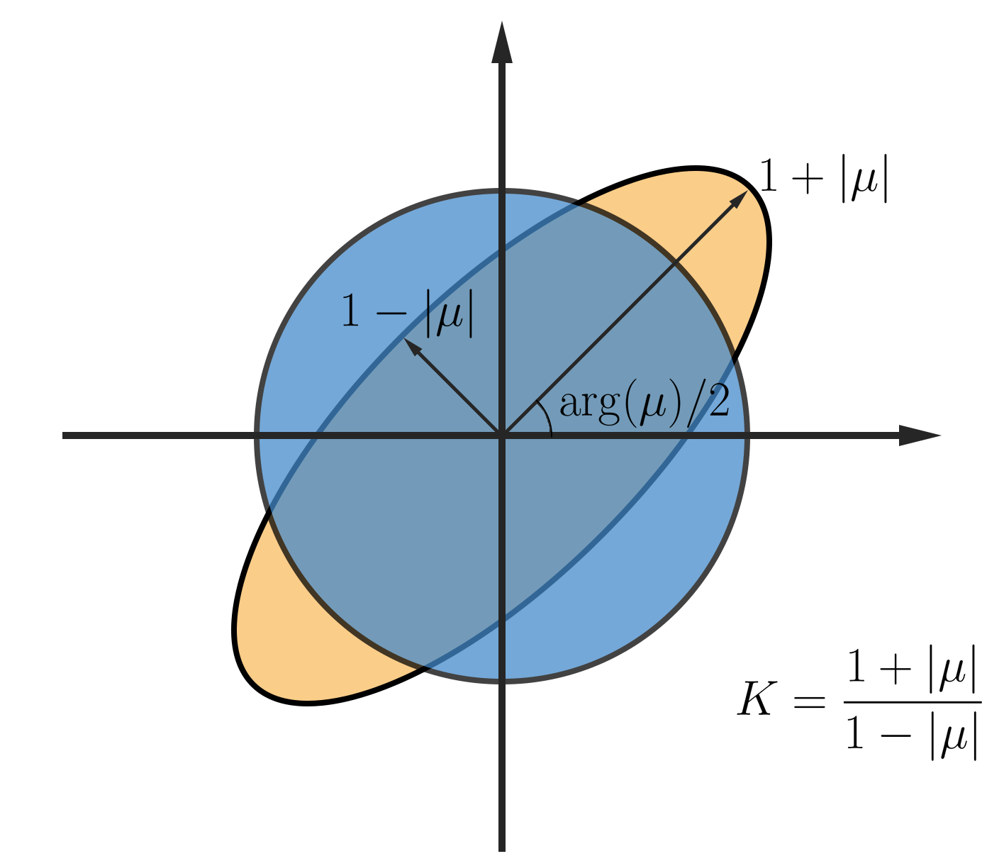
Figure 1: An illustration of the relationship between the conformality distortion and the Beltrami coefficient of a quasi-conformal mapping.

In addition, there is a one-to-one correspondence between the Beltrami coefficient $\mu$ and the quasi-conformal mapping $f$. On one hand, by (1), the Beltrami coefficient $\mu$ can be uniquely calculated if a quasi-conformal mapping $f$ is given. On the other hand, if a Beltrami coefficient $\mu$ is given, the existence and uniqueness of the corresponding quasi-conformal mapping $f$ is established in the following theorem.

Theorem 3.1 (measurable Riemann mapping theorem [16]).

Suppose $\mu:\mathbb{C}\rightarrow\mathbb{C}$ is Lebesgue measurable satisfying $\|\mu\|_{\infty}<1$, then there exists a quasi-conformal mapping $f:\mathbb{C}\rightarrow\mathbb{C}$ in the Sobolev space $W^{1,2}$ that satisfies the Beltrami equation (1) in the distribution sense. Further, assuming that the mapping is stationary at $0,1$, and $\infty$, then the associated quasi-conformal mapping $f$ is uniquely determined.

Further, denote $\sigma_{1}\geq\sigma_{2}>0$ as the singular values of $\nabla f$. Then by (2) again, we have $|\mu(z)|=\frac{\sigma_{1}-\sigma_{2}}{\sigma_{1}+\sigma_{2}}$. Next, we define by $K(z)$ the dilatation

(4) $$K(z)=\frac{1+|\mu(z)|}{1-|\mu(z)|}$$

to express the ratio of the largest singular value of $\nabla f$ divided by the smallest one. So $K(z)$ can also measure how far away the quasi-conformal map at each point is deviated from a conformal map. Hence, based on the above discussion, we can derive a diffeomorphic deformation with bounded geometric distortion by restricting $\mu(z)$ or $K(z)$.

For more details about the quasi-conformal theory, please refer to [16, 29].

3.2 Quasi-conformal registration-based segmentation model

The registration-based segmentation model is to extract the interested region by employing the registration framework. For doing the registration, we require two images, called the template and reference. We can take the target image as the template and prescribe a prior image as the reference, where the structure of the prior image is related to the target image. For example, if the target image has only one object, we can set a disk as the prior image. Ideally, after doing the registration, the boundary of the object in the target image can be linked to the boundary of the object in the prior image by the resulting transformation. Since the prior image is given by users and the location of the boundary of the object in the prior image is known, we can identify the boundary of the interested region in the target image. In addition, if the resulting transformation is one-to-one, a topology-preserving segmentation is guaranteed, which means that the topological structure of the segmentation result is the same with the topological structure of the prior image.

Denote $I(\bm{x}):\Omega\subset\mathbb{R}^{2}\rightarrow\mathbb{R}$ as the target image. For simplicity, we consider two-phase segmentation, namely, segmenting the image domain into the foreground and background. In this way, we can define the prior image as

$$J(c_{1},c_{2},\bm{x})=c_{1}\mathcal{X}_{D}(\bm{x})+c_{2}\mathcal{X}_{D^{c}}(\bm{x}),$$

where $D\subset\Omega$ is a mask, $D^{c}$ is the complement of $D$, and

$$\mathcal{X}_{D}(\bm{x})=\begin{cases}1,\quad\bm{x}\in D\\ 0,\quad\mathrm{otherwise}\end{cases}$$

is the indicator function of $D$. Then, we can build the variational framework of the registration-based segmentation model

$$\min_{c_{1},c_{2},\varphi(\bm{x})}\frac{1}{2}\int_{\Omega}(I(\varphi(\bm{x}))-J(c_{1},c_{2},\bm{x}))^{2}\mathrm{d}\bm{x}+\alpha\mathcal{R}(\varphi(\bm{x})),$$

where $\varphi(\bm{x}):\mathbb{R}^{2}\rightarrow\mathbb{R}^{2}$ is the transformation, $\mathcal{R}(\varphi(\bm{x}))$ is the regularization term to avoid outliers, and $\alpha>0$ is a nonnegative parameter to balance the weight between the fitting term and regularization term.

There exist many choices for the regularizers, such as the elastic regularizer [3], the curvature regularizer [11, 14, 15, 21] and the fractional-order regularizer [55]. However, the most commonly used regularizers can’t ensure a one-to-one transformation because they do not involve the information of the Jacobian determinant of the transformation. Hence, in this paper, to obtain a topology-preserving segmentation model, we mainly consider the following quasi-conformal registration-based segmentation model [4]

(5) $$\min_{c_{1},c_{2},\varphi}\frac{1}{2}\int_{\Omega}(I-J(c_{1},c_{2},\varphi))^{2}\mathrm{d}\bm{x}+\alpha_{1}\int_{\Omega}|\Delta\varphi|^{2}\mathrm{d}\bm{x}+\alpha_{2}\int_{\Omega}\phi(|\mu(\varphi)|^{2})\mathrm{d}\bm{x},$$

where $\Delta$ is the Laplace operator, $|\mu(\varphi)|^{2}$ is computed by (2), $\phi(v)$ is a scaling function defined for positive $v$ which will be chosen in Section 6. This scaling function should scale up the value of $v$ when it approachs $1$ and scale down if it’s near zero. Through this scaling, the value of $v$ should be regularized to be smaller than $1$ as the energy will be dramatically added when $v$ goes toward $1$. $\alpha_{1}$ and $\alpha_{2}$ are nonnegative parameters weighting the two regularization terms. We can see that the second term is to control the smoothness and the third term is to restrict the distortion.

We also want to emphasize that we can interchange the position of the template and reference and obtain an equivalent model

(6) $$\min_{c_{1},c_{2},\varphi}\frac{1}{2}\int_{\Omega}(I(\varphi)-J(c_{1},c_{2}))^{2}\mathrm{d}\bm{x}+\alpha_{1}\int_{\Omega}|\Delta\varphi|^{2}\mathrm{d}\bm{x}+\alpha_{2}\int_{\Omega}\phi(|\mu(\varphi)|^{2})\mathrm{d}\bm{x}.$$

Here, the model (6) is easier to be solved than the model (5) because $c_{1}$, $c_{2}$ and $\varphi$ are decoupled. However, the analysis of the model (5) is more straightforward, which will be illustrated in the following subsection.

4 Revisit on The Fidelity Term of (5)

In order to develop an interactive segmentation model, it is necessary to modify the fidelity term in the segmentation model to incorporate user interaction. In this section, we thoroughly analyze the fidelity term. This analysis will facilitate our development of the interactive segmentation model.

For the fitting term of (5), we set

(7) $$E(c_{1},c_{2},\varphi):=\int_{\Omega}(I-J(c_{1},c_{2},\varphi))^{2}\mathrm{d}\bm{x}=\int_{\Omega}(I-c_{1}\mathcal{X}_{D}\circ\varphi-c_{2}\mathcal{X}_{D^{c}}\circ\varphi)^{2}\mathrm{d}\bm{x}.$$

Since $\varphi$ is a one-to-one mapping, the deformed region $D$ can be set as a region $G$ and $\mathcal{X}_{G}=\mathcal{X}_{D}\circ\varphi$. Hence, (7) can be rewritten as

(8) $$E(c_{1},c_{2},G)=\int_{\Omega}(I-c_{1}\mathcal{X}_{G}-c_{2}\mathcal{X}_{G^{c}})^{2}\mathrm{d}\bm{x}.$$

A segmentation mask $G$ can divide an image domain into a foreground and a background. However, since the segmentation may be imperfect, there could be segmented regions that are not part of the true region of interest, which we call false positive. Those regions that are classified to be the background but are the actual region of interest are called false negative. To simplify our analysis, we can assume two cases: (1) the case with only false positive and (2) the case with only false negative. Thus, we can assume the segmentation result to have three domains, true positive (the correctly segmented foreground), true negative (the correctly segmented background), and false postive/false negative.

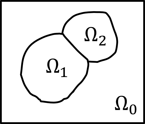
Figure 2: Notations for a three-colored image with three domains: $\Omega_{0}$ (background), $\Omega_{1}$ (foreground - wanted), and $\Omega_{2}$ (foreground - unwanted).

Following these considerations, as Figure 2, we set the image $I$ as follows

(9) $$I=\begin{cases}p_{0},&\bm{x}\in\Omega_{0},\\ p_{1},&\bm{x}\in\Omega_{1},\\ p_{2},&\bm{x}\in\Omega_{2}.\\ \end{cases}$$

Since the domain $\Omega_{0}$ is the background region, minimizing the segmentation energy (8) can lead to three cases: (1)$E(c_{1},c_{2},G=\Omega_{1})$; (2)$E(c_{1},c_{2},G=\Omega_{2})$; (3)$E(c_{1},c_{2},G=\Omega_{1}\cup\Omega_{1})$. Denote the area of some domain $\Omega$ as $||\Omega||$. We can have the following theorem:

Theorem 4.1.

The segmentation energy (8) for a three-colored image $I$ has only three local minimizes. They are

1. $G^{*}=\Omega_{1}$;

2. $G^{*}=\Omega_{2}$;

3. $G^{*}=\Omega_{1}\cup\Omega_{2}$.

This means that no partial of $\Omega_{i}$ can be included.

Proof 4.2.

To prove this, we need to check if there is a case that a partial of $\Omega_{0}$, $\Omega_{1}$ or $\Omega_{2}$ is included in a local minimum. To do so, we investigate the value of $E(G=\mathcal{D}_{0}\cup\mathcal{D}_{1}\cup\mathcal{D}_{2})$, where $\mathcal{D}_{0}\subset\Omega_{0}$, $\mathcal{B}_{0}=\Omega_{0}\setminus\mathcal{D}_{0}$, $\mathcal{D}_{1}\subset\Omega_{1}$, $\mathcal{B}_{1}=\Omega_{1}\setminus\mathcal{D}_{1}$, $\mathcal{D}_{2}\subset\Omega_{2}$ and $\mathcal{B}_{2}=\Omega_{2}\setminus\mathcal{D}_{2}$.

When $G=\mathcal{D}_{0}\cup\mathcal{D}_{1}\cup\mathcal{D}_{2}$, we have

(10) $$c_{1}=\frac{\int_{\mathcal{D}_{0}\cup\mathcal{D}_{1}\cup\mathcal{D}_{2}}I\mathrm{d}\bm{x}}{\int_{\mathcal{D}_{0}\cup\mathcal{D}_{1}\cup\mathcal{D}_{2}}1\mathrm{d}\bm{x}}=\frac{p_{0}||\mathcal{D}_{0}||+p_{1}||\mathcal{D}_{1}||+p_{2}||\mathcal{D}_{2}||}{||\mathcal{D}_{0}||+||\mathcal{D}_{1}||+||\mathcal{D}_{2}||}$$

and

(11) $$c_{2}=\frac{\int_{\mathcal{B}_{0}\cup\mathcal{B}_{1}\cup\mathcal{B}_{2}}I\mathrm{d}\bm{x}}{\int_{\mathcal{B}_{0}\cup\mathcal{B}_{1}\cup\mathcal{B}_{2}}1\mathrm{d}\bm{x}}=\frac{p_{0}||\mathcal{B}_{0}||+p_{1}||\mathcal{B}_{1}||+p_{2}||\mathcal{B}_{2}||}{||\Omega_{0}||+||\mathcal{B}_{1}||+||\mathcal{B}_{2}||}.$$

So we get

(12) $$E(c_{1},c_{2},G=\mathcal{D}_{0}\cup\mathcal{D}_{1}\cup\mathcal{D}_{2}) =\int_{\Omega}(I-c_{1}\mathcal{X}_{\mathcal{D}_{0}\cup\mathcal{D}_{1}\cup\mathcal{D}_{2}}-c_{2}\mathcal{X}_{\mathcal{B}_{0}\cup\mathcal{B}_{1}\cup\mathcal{B}_{2}})^{2}\mathrm{d}\bm{x}$$

$$=\int_{\Omega}((p_{0}-c_{1})\mathcal{X}_{\mathcal{D}_{0}}+(p_{1}-c_{1})\mathcal{X}_{\mathcal{D}_{1}}+(p_{2}-c_{1})\mathcal{X}_{\mathcal{D}_{2}}$$

$$\quad+(p_{0}-c_{2})\mathcal{X}_{\mathcal{B}_{0}}+(p_{1}-c_{2})\mathcal{X}_{\mathcal{B}_{1}}+(p_{2}-c_{2})\mathcal{X}_{\mathcal{B}_{2}})^{2}\mathrm{d}\bm{x}$$

$$=(p_{0}-c_{1})^{2}||\mathcal{D}_{0}||+(p_{1}-c_{1})^{2}||\mathcal{D}_{1}||+(p_{2}-c_{1})^{2}||\mathcal{D}_{2}||$$

$$\quad+(p_{0}-c_{2})^{2}||\mathcal{B}_{0}||+(p_{1}-c_{2})^{2}||\mathcal{B}_{1}||+(p_{2}-c_{2})^{2}||\mathcal{B}_{2}||.$$

We take $A_{0}=||\Omega_{0}||$, $A_{1}=||\Omega_{1}||$, $A_{2}=||\Omega_{2}||$, $B_{0}=||\mathcal{B}_{0}||$, $D_{0}=||\mathcal{D}_{0}||$, $B_{1}=||\mathcal{B}_{1}||$, $D_{1}=||\mathcal{D}_{1}||$, $B_{2}=||\mathcal{B}_{2}||$, $D_{2}=||\mathcal{D}_{2}||$, $d_{12}=|p_{1}-p_{2}|$, $d_{01}=|p_{0}-p_{1}|$ and $d_{02}=|p_{0}-p_{2}|$. Then we can rewrite the above equation as:

(13) $$E(c_{1},c_{2},G) =\frac{((p_{0}-p_{1})D_{1}+(p_{0}-p_{2})D_{2})^{2}}{(D_{0}+D_{1}+D_{2})^{2}}D_{0}+\frac{((p_{1}-p_{0})D_{0}+(p_{1}-p_{2})D_{2})^{2}}{(D_{0}+D_{1}+D_{2})^{2}}D_{1}$$

$$\quad+\frac{((p_{2}-p_{0})D_{0}+(p_{2}-p_{1})D_{1})^{2}}{(D_{0}+D_{1}+D_{2})^{2}}D_{2}+\frac{((p_{0}-p_{1})B_{1}+(p_{0}-p_{2})B_{2})^{2}}{(B_{0}+B_{1}+B_{2})^{2}}B_{0}$$

$$\quad+\frac{((p_{1}-p_{0})B_{0}+(p_{1}-p_{2})B_{2})^{2}}{(B_{0}+B_{1}+B_{2})^{2}}B_{1}+\frac{((p_{2}-p_{0})B_{0}+(p_{2}-p_{1})B_{1})^{2}}{(B_{0}+B_{1}+B_{2})^{2}}B_{2}$$

$$=\frac{d_{12}^{2}D_{1}D_{2}+d_{01}^{2}D_{0}D_{1}+d_{02}^{2}D_{0}D_{2}}{D_{0}+D_{1}+D_{2}}+\frac{d_{12}^{2}B_{1}B_{2}+d_{01}^{2}B_{0}B_{1}+d_{02}^{2}B_{0}B_{2}}{B_{0}+B_{1}+B_{2}}$$

$$=d_{12}^{2}(D_{2}-\frac{D_{0}D_{2}+D_{2}^{2}}{D_{0}+D_{1}+D_{2}})+d_{01}^{2}(D_{0}-\frac{D_{0}^{2}+D_{0}D_{2}}{D_{0}+D_{1}+D_{2}})+d_{02}^{2}\frac{D_{0}D_{2}}{D_{0}+D_{1}+D_{2}}$$

$$\quad+d_{12}^{2}(B_{2}-\frac{B_{0}B_{2}+B_{2}^{2}}{B_{0}+B_{1}+B_{2}})+d_{01}^{2}(B_{0}-\frac{B_{0}^{2}+B_{0}B_{2}}{B_{0}+B_{1}+B_{2}})+d_{02}^{2}\frac{B_{0}B_{2}}{B_{0}+B_{1}+B_{2}}$$

$$=d_{12}^{2}(D_{2}-\frac{D_{0}D_{2}+D_{2}^{2}}{D_{0}+A_{1}+D_{2}-B_{1}})+d_{01}^{2}(D_{0}-\frac{D_{0}^{2}+D_{0}D_{2}}{D_{0}+A_{1}+D_{2}-B_{1}})$$

$$\quad+d_{02}^{2}\frac{D_{0}D_{2}}{D_{0}+A_{1}+D_{2}-B_{1}}$$

$$\quad+d_{12}^{2}(B_{2}-\frac{B_{0}B_{2}+B_{2}^{2}}{B_{0}+B_{1}+B_{2}})+d_{01}^{2}(B_{0}-\frac{B_{0}^{2}+B_{0}B_{2}}{B_{0}+B_{1}+B_{2}})+d_{02}^{2}\frac{B_{0}B_{2}}{B_{0}+B_{1}+B_{2}}.$$

Treating $B_{0}$, $B_{1}$, $B_{2}$ as three variables, we can have $B_{0}\in[0,A_{0}]$, $B_{1}\in[0,A_{1}]$, $B_{2}\in[0,A_{2}]$ as $\mathcal{B}_{0}\subset\Omega_{0}$, $\mathcal{B}_{1}\subset\Omega_{1}$, $\mathcal{B}_{2}\subset\Omega_{2}$. Naturally, $D_{0}=A_{0}-B_{0}$, $D_{1}=A_{1}-B_{1}$, $D_{2}=A_{2}-B_{2}$. Further, define a function:

(14) $$F(B_{0},B_{1},B_{2})=E(c_{1},c_{2},G=\mathcal{D}_{0}\cup\mathcal{D}_{1}\cup\mathcal{D}_{2}).$$

We then compute $\frac{\partial F}{\partial B_{1}}$:

(15) $$\frac{\partial F}{\partial B_{1}} =-\frac{d_{12}^{2}(D_{0}D_{2}+D_{2}^{2})+d_{01}^{2}(D_{0}^{2}+D_{0}D_{2})-d_{02}^{2}D_{0}D_{2}}{(D_{0}+A_{1}+D_{2}-B_{1})^{2}}$$

$$\quad+\frac{d_{12}^{2}(B_{0}B_{2}+B_{2}^{2})+d_{01}^{2}(B_{0}^{2}+B_{0}B_{2})-d_{02}^{2}B_{0}B_{2}}{(B_{0}+B_{1}+B_{2})^{2}}.$$

By definition of $d_{12}$, $d_{01}$ and $d_{02}$, we have $(d_{01}+d_{12})^{2}\geq d_{02}^{2}$ and $d_{01}^{2}+d_{12}^{2}\geq 2d_{01}d_{02}$. Thus, we obtain

$$\begin{split}&d_{12}^{2}(B_{0}B_{2}+B_{2}^{2})+d_{01}^{2}(B_{0}^{2}+B_{0}B_{2})-d_{02}^{2}B_{0}B_{2}\\ \geq&d_{12}^{2}B_{0}B_{2}+d_{01}^{2}B_{0}B_{2}+2d_{12}d_{01}B_{0}B_{2}-d_{02}^{2}B_{0}B_{2}\\ =&(d_{01}+d_{12})^{2}B_{0}B_{2}-d_{02}^{2}B_{0}B_{2}\geq 0\end{split}$$

and

$$\begin{split}&d_{12}^{2}(D_{0}D_{2}+D_{2}^{2})+d_{01}^{2}(D_{0}^{2}+D_{0}D_{2})-d_{02}^{2}D_{0}D_{2}\\ \geq&d_{12}^{2}D_{0}D_{2}+d_{01}^{2}D_{0}D_{2}+2d_{12}d_{01}D_{0}D_{2}-d_{02}^{2}D_{0}D_{2}\\ =&(d_{01}+d_{12})^{2}D_{0}D_{2}-d_{02}^{2}D_{0}D_{2}\geq 0.\end{split}$$

Hence, both the first term and the second term of $\frac{\partial F}{\partial B_{1}}$ are monotonously decreasing for any $B_{1}\in(0,A_{1})$ given a fixed $B_{0}\in(0,A_{0})$ and $B_{2}\in(0,A_{2})$.

As $\frac{\partial F}{\partial B_{1}}$ is monotonously decreasing for any given $B_{0}$ and $B_{2}$, there is at most one maximum within $B_{1}\in(0,A_{1})$ for any given $B_{0}$ and $B_{2}$. The minimum of $F(B_{0},B_{1},B_{2})$ must only be obtained when $B_{1}=0$ or $B_{1}=A_{1}$ for any given $B_{0}$ and $B_{2}$. So is for $B_{2}$ given any $B_{0}$ and $B_{1}$. Thus, the minimum can never be obtained when partial of the domain $\Omega_{i}$ is included.

Next, we compute the corresponding energy value with respect to these different cases. When $G=\Omega_{1}$, we have $c_{1}=\frac{\int_{\Omega_{1}}I\mathrm{d}\bm{x}}{\int_{\Omega_{1}}1\mathrm{d}\bm{x}}=p_{1}$ and $c_{2}=\frac{\int_{\Omega_{1}^{c}}I\mathrm{d}\bm{x}}{\int_{\Omega_{1}^{c}}1\mathrm{d}\bm{x}}=\frac{p_{2}||\Omega_{2}||+p_{0}||\Omega_{0}||}{||\Omega_{2}||+||\Omega_{0}||}$. Then, we can get

(16) $$E(c_{1},c_{2},G=\Omega_{1}) =\int_{\Omega}(I-c_{1}\mathcal{X}_{\Omega_{1}}-c_{2}\mathcal{X}_{\Omega_{2}\cup\Omega_{0}})^{2}\mathrm{d}\bm{x}$$

$$=\int_{\Omega}(p_{0}\mathcal{X}_{\Omega_{0}}+p_{1}\mathcal{X}_{\Omega_{1}}+p_{2}\mathcal{X}_{\Omega_{2}}-p_{1}\mathcal{X}_{\Omega_{1}}-c_{2}\mathcal{X}_{\Omega_{0}}-c_{2}\mathcal{X}_{\Omega_{2}})^{2}\mathrm{d}\bm{x}$$

$$=\int_{\Omega}|(p_{0}-c_{2})\mathcal{X}_{\Omega_{0}}+(p_{2}-c_{2})\mathcal{X}_{\Omega_{2}}|^{2}\mathrm{d}\bm{x}$$

$$=(p_{0}-c_{2})^{2}\int_{\Omega}|\mathcal{X}_{\Omega_{0}}|^{2}\mathrm{d}\bm{x}+(p_{2}-c_{2})^{2}\int_{\Omega}|\mathcal{X}_{\Omega_{2}}|^{2}\mathrm{d}\bm{x}$$

$$=(p_{0}-c_{2})^{2}||\Omega_{0}||+(p_{2}-c_{2})^{2}||\Omega_{2}||$$

$$=\left(\frac{p_{0}||\Omega_{2}||-p_{2}||\Omega_{2}||}{||\Omega_{2}||+||\Omega_{0}||}\right)^{2}||\Omega_{0}||+\left(\frac{p_{2}||\Omega_{0}||-p_{0}||\Omega_{0}||}{||\Omega_{2}||+||\Omega_{0}||}\right)^{2}||\Omega_{2}||$$

$$=(p_{0}-p_{2})^{2}\frac{||\Omega_{2}||||\Omega_{0}||}{||\Omega_{2}||+||\Omega_{0}||}.$$

Similarly, when $G=\Omega_{2}$, we have $c_{1}=\frac{\int_{\Omega_{2}}I\mathrm{d}\bm{x}}{\int_{\Omega_{2}}1\mathrm{d}\bm{x}}=p_{2}$, $c_{2}=\frac{\int_{\Omega_{2}^{c}}I\mathrm{d}\bm{x}}{\int_{\Omega_{2}^{c}}1\mathrm{d}\bm{x}}=\frac{p_{1}||\Omega_{1}||+p_{0}||\Omega_{0}||}{||\Omega_{1}||+||\Omega_{0}||}$, and

(17) $$E(c_{1},c_{2},G=\Omega_{2}) =\int_{\Omega}(I-c_{1}\mathcal{X}_{\Omega_{2}}-c_{2}\mathcal{X}_{\Omega_{1}\cup\Omega_{0}})^{2}\mathrm{d}\bm{x}$$

$$=(p_{0}-p_{1})^{2}\frac{||\Omega_{1}||||\Omega_{0}||}{||\Omega_{1}||+||\Omega_{0}||}.$$

And for $G=\Omega_{1}\cup\Omega_{2}$, we get $c_{1}=\frac{\int_{\Omega_{1}\cup\Omega_{2}}I\mathrm{d}\bm{x}}{\int_{\Omega_{1}\cup\Omega_{2}}1\mathrm{d}\bm{x}}=\frac{p_{1}||\Omega_{1}||+p_{2}||\Omega_{2}||}{||\Omega_{1}||+||\Omega_{2}||}$, $c_{2}=\frac{\int_{\Omega_{0}}I\mathrm{d}\bm{x}}{\int_{\Omega_{0}}1\mathrm{d}\bm{x}}=p_{0}$, and

(18) $$E(c_{1},c_{2},G=\Omega_{1}\cup\Omega_{2}) =\int_{\Omega}(I-c_{1}\mathcal{X}_{\Omega_{1}\cup\Omega_{2}}-c_{2}\mathcal{X}_{\Omega_{0}})^{2}\mathrm{d}\bm{x}$$

$$=(p_{1}-p_{2})^{2}\frac{||\Omega_{1}||||\Omega_{2}||}{||\Omega_{1}||+||\Omega_{2}||}.$$

For a clear three-colored image, we can optimize the energy functional (8) and obtain $G^{*}$ by comparing the energy values of the above three cases:

• $G^{*}=\Omega_{1}$, if

  (19) $$\begin{cases}(p_{0}-p_{2})^{2}\frac{||\Omega_{2}||}{||\Omega_{2}||+||\Omega_{0}||}\leq(p_{0}-p_{1})^{2}\frac{||\Omega_{1}||}{||\Omega_{1}||+||\Omega_{0}||},\\ (p_{0}-p_{2})^{2}\frac{||\Omega_{0}||}{||\Omega_{2}||+||\Omega_{0}||}\leq(p_{1}-p_{2})^{2}\frac{||\Omega_{1}||}{||\Omega_{1}||+||\Omega_{2}||}.\end{cases}$$

• $G^{*}=\Omega_{2}$, if

  (20) $$\begin{cases}(p_{0}-p_{1})^{2}\frac{||\Omega_{1}||}{||\Omega_{1}||+||\Omega_{0}||}\leq(p_{0}-p_{2})^{2}\frac{||\Omega_{2}||}{||\Omega_{2}||+||\Omega_{0}||},\\ (p_{0}-p_{1})^{2}\frac{||\Omega_{0}||}{||\Omega_{1}||+||\Omega_{0}||}\leq(p_{1}-p_{2})^{2}\frac{||\Omega_{2}||}{||\Omega_{1}||+||\Omega_{2}||}.\end{cases}$$

• $G^{*}=\Omega_{1}\cup\Omega_{2}$, if

  (21) $$\begin{cases}(p_{1}-p_{2})^{2}\frac{||\Omega_{1}||}{||\Omega_{1}||+||\Omega_{2}||}\leq(p_{0}-p_{2})^{2}\frac{||\Omega_{0}||}{||\Omega_{2}||+||\Omega_{0}||},\\ (p_{1}-p_{2})^{2}\frac{||\Omega_{2}||}{||\Omega_{1}||+||\Omega_{2}||}\leq(p_{0}-p_{1})^{2}\frac{||\Omega_{0}||}{||\Omega_{1}||+||\Omega_{0}||}.\end{cases}$$

Theorem 4.3.

The minimizer $G^{*}$ for the segmentation energy (8) for a clear three-colored image $I$ is one of the following three:

1. $G^{*}=\Omega_{1}$, when (19) is satisfied;

2. $G^{*}=\Omega_{2}$, when (20) is satisfied;

3. $G^{*}=\Omega_{1}\cup\Omega_{2}$, when (21) is satisfied.

5 Method

In this section, we describe our proposed Quasi-conformal Interactive Segmentation model in detail.

5.1 Overall Description

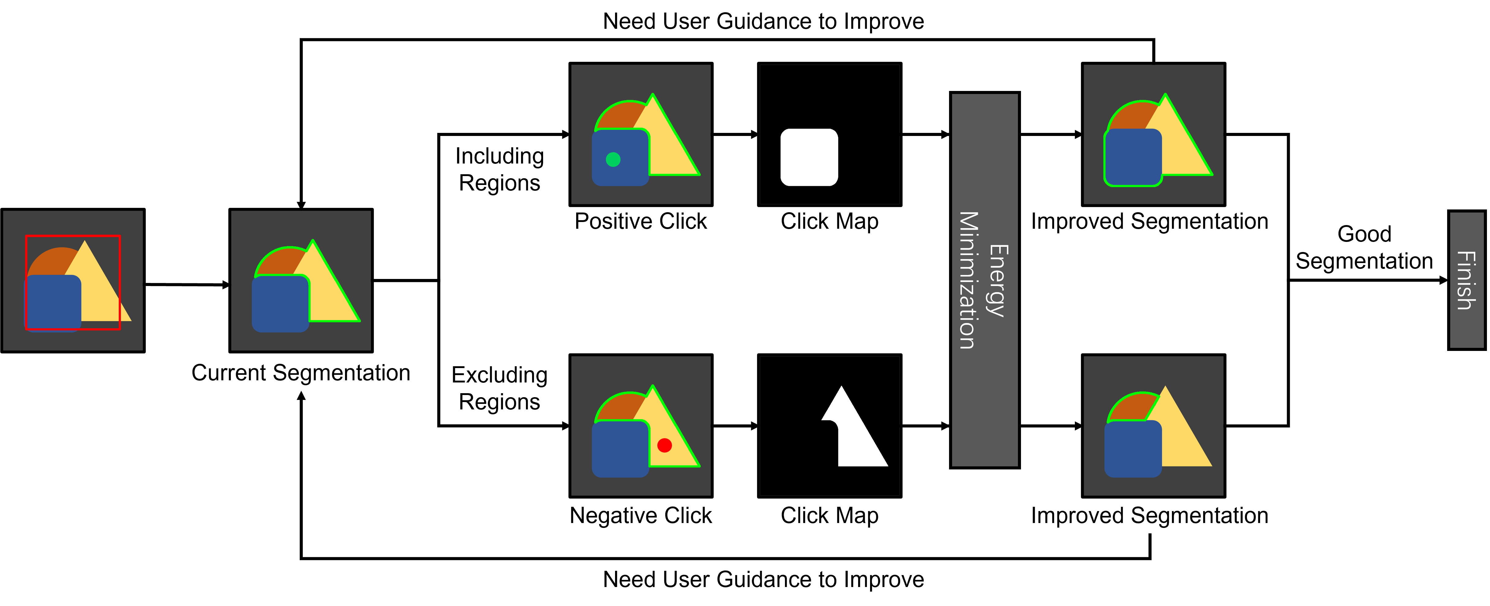
Figure 3: A flow chart illustrating the process of the quasiconformal interactive segmentation (QIS) model.

In this subsection, we provide an overview of the interactive segmentation procedure. Figure 3 visually illustrates the process. Initially, the Quasi-conformal registration-based segmentation model, described in (6), is applied to obtain an initial segmentation. This initial segmentation serves as the current segmentation mask, which may not be entirely accurate and thus requires further adjustments. To guide these adjustments, the user can indicate regions to be included (using positive clicks) and regions to be excluded (using negative clicks). These clicks are then converted into a click map, which is subsequently incorporated into the Quasi-conformal segmentation model. By minimizing the interactive segmentation energy, a segmentation Quasi-conformal map is generated, resulting in an improved segmentation mask. If the improved segmentation is not satisfactory, the process is repeated until a satisfactory segmentation result is achieved. This iterative procedure, which incorporates the user’s input, is referred to as the interactive segmentation process.

In the following subsections, we will discuss the definitions of positive clicks, negative clicks, and click maps in details. Additionally, we will provide a comprehensive explanation of the proposed interactive segmentation fidelity term. This fidelity term is a crucial component that is integrated into the Quasi-conformal segmentation model, specifically designed for interactive segmentation purposes.

5.2 Click map

In this subsection, we introduce the click map, which is essential for constructing our proposed interactive segmentation model.

Mis-segmentation may result in the exclusion of certain regions from the segmentation mask. To address this, users actively participate in the process by interactively delineating points within these excluded regions. These points are referred to as positive clicks. We denote the collection of positive clicks by $C_{p}$. Similarly, there may be instances where regions that do not belong to the object of interest are mistakenly included in the segmentation mask. To address this, users assist by delineating points within these regions. These points are referred to as negative clicks, as they indicate areas that should be excluded from the final segmentation. The collection of negative clicks is denoted as $C_{n}$.

The concepts of positive clicks and negative clicks are introduced to minimize the level of user intervention required in identifying specific regions for inclusion or exclusion. From these clicks, a click map can be generated, which effectively captures the local homogeneous regions that are grown around the user’s clicks. These local homogeneous regions approximate the regions to be included for positive clicks and the regions to be excluded for negative clicks. This approach ultimately enhances the user experience by streamlining the segmentation process and significantly reducing the manual intervention required.

In this work, we propose a methodology to generate the click map from user clicks based on $K$-means clustering. Suppose a collection $\mathcal{C}_{*}$ of positive clicks or negative clicks is given. In other words, $\mathcal{C}_{*}=\mathcal{C}_{p}$ or $\mathcal{C}_{n}$. The image domain $\Omega$ can be decomposed into $K$ clusters based on the image intensity $I:\Omega\to\mathbb{R}$, using the $K$-means clustering. Mathematically, we divide $\Omega$ into $K$ sets, namely, $\mathcal{K}_{1}$, $\mathcal{K}_{2}$, $\dots$, $\mathcal{K}_{K}$ by mininizing the intra-cluster variance:

(22) $$\min_{\mathcal{K}_{1},\cdots,\mathcal{K}_{K}}\sum_{i=1}^{K}\sum_{\bm{x}\in\mathcal{K}_{i}}\|I(\bm{x})-I(\bm{\mu}_{i})\|^{2},$$

where $\bm{\mu}_{i}$ is the centroid of the cluster $i$. This expression quantifies the similarity of data points within each cluster. The $K$-means clustering can be computed using the following algorithm.

Algorithm 1 K-means Clustering Segmentation

  Choose the number of clusters $K$;

  Randomly select $K$ points from $\Omega$ as $\bm{\mu}_{1}$,$\dots$,$\bm{\mu}_{K}$;

  for $l=1:\text{MaxKS}$ do

     Solve (22) to obtain $\mathcal{K}_{1}$, $\cdots$, $\mathcal{K}_{K}$;

     Recompute $\bm{\mu}_{i}$ to be the centroid of $\mathcal{K}_{i}$ for each $i$;

     if stopping criteria is satisfied then

        berak;

     end if

  end for

Note that each cluster $\mathcal{K}_{i}$, may consist of multiple isolated components. We denote the isolated components by $D^{i}_{j}$. Hence, $\mathcal{K}_{i}=\bigcup_{j=1}^{N_{i}}D^{i}_{j}$, where $N_{i}$ indicates the number of isolated regions within cluster $i$. For each $\bm{x}_{\text{click}}\in\mathcal{C}_{*}$, we define $\delta(\bm{x}_{click})$ as follows:

(23) $$\delta(\bm{x}_{click})={D^{i}_{j}}\text{ for }(i,j)\text{ if }\bm{x}_{click}\in D^{i}_{j}.$$

A local homogeneous region surrounding clicks can be obtained by taking the union, which is given by $\mathcal{H}=\bigcup_{\bm{x}_{click}\in\mathcal{C}_{*}}\delta(\bm{x}_{click})$. A click map $M_{\text{click}}$, which is a binary map capturing $\mathcal{H}$, can be defined as follows.

Definition 5.1 (Click map).

The click map $M_{\text{clicks}}$ for clicks $\mathcal{C}_{*}$ is defined as:

(24) $$M_{\text{clicks}}(\bm{x})=\begin{cases}1,&\text{if }\bm{x}\in\mathcal{H},\\ 0,&\text{otherwise}.\end{cases}$$

Note that the definition provided above accommodates not only single clicks but also sets of clicks as input. This formulation enables the convenient use of drawing continuous lines instead of individual clicks, which can be directly converted into a collection of densely sampled points along the line. This approach enhances the efficiency of providing guidance.

5.3 Fidelity Term for Interactive Segmentation

The click map provide additional information to refine the segmentation prediction. In this subsection, we will outline how the click map can be effectively integrated into the quasiconformal segmentation model, specifically through the use of a special fidelity term designed for interactive segmentation.

Given a click map $M_{\mathrm{clicks}}:\Omega\longrightarrow\mathbb{R}$, our proposed interactive segmentation fidelity energy as

(25) $$E_{int}(c_{1},c_{2},G;M_{\mathrm{clicks}})=\int_{\Omega}(I+rM_{\mathrm{clicks}}-c_{1}\mathcal{X}_{G}-c_{2}\mathcal{X}_{G^{c}})^{2}\mathrm{d}\bm{x}.$$

With a carefully selected value of $r$ for the provided click map $M_{\mathrm{clicks}}$, the new energy functional (25) is designed to facilitate the inclusion or exclusion of specific regions within the initial segmentation. In the following, we will examine two scenarios. The first scenario involves including the false negative region, which should have been part of the segmentation but was erroneously omitted from the initial segmentation mask. The second scenario involves excluding the false positive region, which is not relevant to the region of interest but was mistakenly included in the initial segmentation mask.

5.3.1 Positive click

When the initial segmentation generated by the model (8) includes only a portion of the region of interest, additional interaction is required to provide information about the missed areas. These missed areas are referred to as false negatives, and we aim to address them through user interaction. Therefore, we call this type of interaction as a positive click, as it is intended to rectify the false negative regions and incorporate them into the segmentation.

Mathematically, suppose the region of interest is represented by the union of two regions, $\Omega_{1}\cup\Omega_{2}$. However, the initial segmentation only identifies $\Omega_{1}$, omitting the presence of $\Omega_{2}$. To rectify this, a positive click is required to indicate that $\Omega_{2}$ should also be included as part of the region of interest. Therefore, by leveraging the interactive segmentation fidelity energy, the parameter $r$ in (25) needs to be carefully selected to ensure that the updated model can generate an optimal segmentation $G^{**}=\Omega_{1}\cup\Omega_{2}$. The following theorem describes how $r$ can be chosen.

Theorem 5.2.

Given a three-colored image $I$ defined as (9), with the initial segmentation $G^{*}=\Omega_{1}$ derived by (8) and the click map $M_{\mathrm{clicks}}=\mathcal{X}_{\Omega_{2}}$, we can obtain the desired segmentation $G^{**}=\Omega_{1}\cup\Omega_{2}$ from the interactive segmentation fidelity energy (27) if $r$ satisfies (38).

Proof 5.3.

Since the initial segmentation is $\Omega_{1}$, we know that $G^{*}=\Omega_{1}$ can make the original energy functional (8) reach its minimal. Thus, we can refer to (19) and obtain

$$\begin{cases}(p_{0}-p_{2})^{2}\frac{||\Omega_{2}||}{||\Omega_{2}||+||\Omega_{0}||}\leq(p_{0}-p_{1})^{2}\frac{||\Omega_{1}||}{||\Omega_{1}||+||\Omega_{0}||},\\ (p_{0}-p_{2})^{2}\frac{||\Omega_{0}||}{||\Omega_{2}||+||\Omega_{0}||}\leq(p_{1}-p_{2})^{2}\frac{||\Omega_{1}||}{||\Omega_{1}||+||\Omega_{2}||}.\end{cases}$$

Suppose the click map acquired by the positive click assigned on $\Omega_{2}$ is perfect, which means that the click map is $M_{\mathrm{clicks}}=\mathcal{X}_{\Omega_{2}}$. Bringing it into the interactive segmentation fidelity energy (25), we hope to get a segmentation $G^{**}=\Omega_{1}\cup\Omega_{2}$ under a properly chosen $r$. Alternatively speaking, we hope that the following conditions are satisfied

(26) $$\begin{cases}E_{int}(c_{1},c_{2},G=\Omega_{1}\cup\Omega_{2};M_{\mathrm{clicks}}=\mathcal{X}_{\Omega_{2}})\leq E_{int}(c_{1},c_{2},G=\Omega_{1};M_{\mathrm{clicks}}=\mathcal{X}_{\Omega_{2}}),\\ E_{int}(c_{1},c_{2},G=\Omega_{1}\cup\Omega_{2};M_{\mathrm{clicks}}=\mathcal{X}_{\Omega_{2}})\leq E_{int}(c_{1},c_{2},G=\Omega_{2};M_{\mathrm{clicks}}=\mathcal{X}_{\Omega_{2}}).\end{cases}$$

Note that for the computation of $E_{int}$, we can do some transformations as

(27) $$\begin{split}E_{int}(c_{1},c_{2},G;M_{\mathrm{clicks}})&=\int_{\Omega}|I+rM_{\mathrm{clicks}}-c_{1}\mathcal{X}_{G}-c_{2}\mathcal{X}_{G^{c}}|^{2}\mathrm{d}\bm{x}\\ &=\int_{\Omega}|I^{*}-c_{1}\mathcal{X}_{G}-c_{2}\mathcal{X}_{G^{c}}|^{2}\mathrm{d}\bm{x},\end{split}$$

where

(28) $$I^{*}=\begin{cases}p_{0},&\ (x,y)\in\Omega_{0},\\ p_{1},&\ (x,y)\in\Omega_{1},\\ p_{2}+r,&\ (x,y)\in\Omega_{2}.\\ \end{cases}$$

The second equation in (27) is similar to (8), then we can directly replace $p_{2}$ with $p_{2}+r$ in (16), (17) and (18) to obtain

(29) $$E_{int}(c_{1},c_{2},G=\Omega_{1};M_{\mathrm{clicks}}=\mathcal{X}_{\Omega_{2}})=(p_{0}-p_{2}-r)^{2}\frac{||\Omega_{2}||||\Omega_{0}||}{||\Omega_{2}||+||\Omega_{0}||},$$

$$E_{int}(c_{1},c_{2},G=\Omega_{2};M_{\mathrm{clicks}}=\mathcal{X}_{\Omega_{2}})=(p_{0}-p_{1})^{2}\frac{||\Omega_{1}||||\Omega_{0}||}{||\Omega_{1}||+||\Omega_{0}||},$$

$$E_{int}(c_{1},c_{2},G=\Omega_{1}\cup\Omega_{2};M_{\mathrm{clicks}}=\mathcal{X}_{\Omega_{2}})=(p_{1}-p_{2}-r)^{2}\frac{||\Omega_{1}||||\Omega_{2}||}{||\Omega_{1}||+||\Omega_{2}||}.$$

Substituting (29) into (26), we obtain

(30) $$\begin{cases}(p_{1}-p_{2}-r)^{2}\frac{||\Omega_{1}||}{||\Omega_{1}||+||\Omega_{2}||}\leq(p_{0}-p_{2}-r)^{2}\frac{||\Omega_{0}||}{||\Omega_{2}||+||\Omega_{0}||},\\ (p_{1}-p_{2}-r)^{2}\frac{||\Omega_{2}||}{||\Omega_{1}||+||\Omega_{2}||}\leq(p_{0}-p_{1})^{2}\frac{||\Omega_{0}||}{||\Omega_{1}||+||\Omega_{0}||}.\end{cases}$$

For the first inequality in (30), we have

$$(p_{1}-p_{2}-r)^{2}\frac{||\Omega_{1}||(||\Omega_{2}||+||\Omega_{0}||)}{||\Omega_{0}||(||\Omega_{1}||+||\Omega_{2}||)}\leq(p_{0}-p_{2}-r)^{2}.$$

Taking $A=\sqrt{\frac{||\Omega_{1}||(||\Omega_{2}||+||\Omega_{0}||)}{||\Omega_{0}||(||\Omega_{1}||+||\Omega_{2}||)}}$, we get

(31) $$((p_{1}-p_{2})A-(p_{0}-p_{2})-(A-1)r)((p_{1}-p_{2})A+(p_{0}-p_{2})-(A+1)r)\leq 0.$$

For $A\neq 1$, we further obtain

$$(A-1)(A+1)\left(\frac{(p_{1}-p_{2})A-(p_{0}-p_{2})}{(A-1)}-r\right)\left(\frac{(p_{1}-p_{2})A+(p_{0}-p_{2})}{(A+1)}-r\right)\leq 0.$$

Set $R_{x}=\frac{(p_{1}-p_{2})A-(p_{0}-p_{2})}{A-1}$ and $R_{y}=\frac{(p_{1}-p_{2})A+(p_{0}-p_{2})}{A+1}$. Note that here there can never be $p_{1}=p_{0}$, or they should be in the same region for an object in the image. So we have

• when $A>1$ ($||\Omega_{1}||>||\Omega_{0}||$),

  (32) $$\begin{cases}R_{x}\leq r\leq R_{y}\ \text{when $p_{0}>p_{1}$},\\ R_{y}\leq r\leq R_{x}\ \text{when $p_{0}<p_{1}$}.\\ \end{cases}$$

• when $0<A<1$ ($||\Omega_{1}||<||\Omega_{0}||$),

  (33) $$\begin{cases}r\leq R_{y}\text{ or }R_{x}\leq r\ \text{when $p_{0}>p_{1}$}.\\ r\leq R_{x}\text{ or }R_{y}\leq r\ \text{when $p_{0}<p_{1}$},\\ \end{cases}$$

For $A=1$ ($||\Omega_{1}||=||\Omega_{0}||$), by (31), we get

(34) $$(p_{1}-p_{0})\left(\frac{p_{1}+p_{0}-2p_{2}}{2}-r\right)\leq 0.$$

Since $R_{y}=\frac{p_{1}+p_{0}-2p_{2}}{2}$ when $A=1$, thus we have

(35) $$\begin{cases}R_{y}\geq r\ \text{when $p_{0}>p_{1}$},\\ R_{y}\leq r\ \text{when $p_{0}<p_{1}$}.\\ \end{cases}$$

For the second inequality in (30), it can lead to

$$(p_{1}-p_{2}-r)^{2}\frac{||\Omega_{2}||(||\Omega_{1}||+||\Omega_{0}||)}{||\Omega_{0}||(||\Omega_{1}||+||\Omega_{2}||)}\leq(p_{0}-p_{1})^{2}.$$

Taking $B=\sqrt{\frac{||\Omega_{2}||(||\Omega_{1}||+||\Omega_{0}||)}{||\Omega_{0}||(||\Omega_{1}||+||\Omega_{2}||)}}$, we have

$$\left(\frac{(p_{1}-p_{2})B+(p_{0}-p_{1})}{B}-r\right)\left(\frac{(p_{1}-p_{2})B-(p_{0}-p_{1})}{B}-r\right)\leq 0.$$

Set $Q_{x}=\frac{(p_{1}-p_{2})B-(p_{0}-p_{1})}{B}$ and $Q_{y}=\frac{(p_{1}-p_{2})B+(p_{0}-p_{1})}{B}$, then we get

(36) $$\begin{cases}Q_{x}\leq r\leq Q_{y}\ \text{when $p_{0}>p_{1}$},\\ Q_{y}\leq r\leq Q_{x}\ \text{when $p_{0}<p_{1}$}.\\ \end{cases}$$

It is easy to find the relation among $R_{x}$, $Q_{x}$, $R_{y}$ and $Q_{y}$,

(37) $$\begin{cases}R_{x}\leq Q_{x}\leq R_{y}\leq Q_{y}\ \text{when $A>1$ and $p_{0}>p_{1}$},\\ Q_{y}\leq R_{y}\leq Q_{x}\leq R_{x}\ \text{when $A>1$ and $p_{0}<p_{1}$},\\ Q_{x}\leq R_{y}\leq Q_{y}\leq R_{x}\ \text{when $1>A>0$ and $p_{0}>p_{1}$},\\ R_{x}\leq Q_{y}\leq R_{y}\leq Q_{x}\ \text{when $1>A>0$ and $p_{0}<p_{1}$},\\ Q_{x}\leq R_{y}\leq Q_{y}\ \text{when $A=1$ and $p_{0}>p_{1}$},\\ Q_{y}\leq R_{y}\leq Q_{x}\ \text{when $A=1$ and $p_{0}<p_{1}$}.\\ \end{cases}$$

Hence, the model (25) will give an optimal segmentation $G^{**}=\Omega_{1}\cup\Omega_{2}$ if the parameter $r$ satisfies the following condition

(38) $$\begin{cases}Q_{x}\leq r\leq R_{y}\ \text{when $p_{0}>p_{1}$},\\ R_{y}\leq r\leq Q_{x}\ \text{when $p_{0}<p_{1}$}.\end{cases}$$

which also motivates us to calculate $r$ as the middle point of the range, i.e. $r=(R_{y}+Q_{x})/2$.

5.3.2 Negative click

When the initial segmentation generated by (8) includes an additional region that is not part of the desired segmentation, known as a false positive, a negative click is required to remove it. Assume that the region of interest is denoted as $\Omega_{1}$, but the initial segmentation erroneously includes an extra region $\Omega_{2}$. By considering the click map $M_{\mathrm{clicks}}=\mathcal{X}_{\Omega_{2}}$, we need to carefully choose the parameter $r$ in (25) to ensure that the updated model can produce an optimal segmentation $G^{**}=\Omega_{1}$. The following theorem provides details on how the value of $r$ can be selected.

Theorem 5.4.

Given a three-colored image $I$ defined as (9), with the initial segmentation $G^{*}=\Omega_{1}\cup\Omega_{2}$ derived from (8) and the click map $M_{\mathrm{clicks}}=\mathcal{X}_{\Omega_{2}}$, we can obtain the desired segmentation $G^{**}=\Omega_{1}$ from the interactive segmentation fidelity energy (27) if $r$ satisfies (48).

Proof 5.5.

Since the initial segmentation is $\Omega_{1}\cup\Omega_{2}$, we can know that $G^{*}=\Omega_{1}\cup\Omega_{2}$ can make the original energy function (8) reach its minimal. Following (21), we obtain

(39) $$\begin{cases}(p_{1}-p_{2})^{2}\frac{||\Omega_{1}||}{||\Omega_{1}||+||\Omega_{2}||}\leq(p_{0}-p_{2})^{2}\frac{||\Omega_{0}||}{||\Omega_{2}||+||\Omega_{0}||},\\ (p_{1}-p_{2})^{2}\frac{||\Omega_{2}||}{||\Omega_{1}||+||\Omega_{2}||}\leq(p_{0}-p_{1})^{2}\frac{||\Omega_{0}||}{||\Omega_{1}||+||\Omega_{0}||}.\end{cases}$$

Bringing the click map $M_{\mathrm{clicks}}=\mathcal{X}_{\Omega_{2}}$ into the interactive segmentation fidelity energy (25), we hope to get a segmentation $G^{**}=\Omega_{1}$ under a properly chosen $r$. Namely, the following conditions should be satisfied

(40) $$\begin{cases}E_{int}(c_{1},c_{2},G=\Omega_{1};M_{\mathrm{clicks}}=\mathcal{X}_{\Omega_{2}})\leq E_{int}(c_{1},c_{2},G=\Omega_{1}\cup\Omega_{2};M_{\mathrm{clicks}}=\mathcal{X}_{\Omega_{2}}),\\ E_{int}(c_{1},c_{2},G=\Omega_{1};M_{\mathrm{clicks}}=\mathcal{X}_{\Omega_{2}})\leq E_{int}(c_{1},c_{2},G=\Omega_{2};M_{\mathrm{clicks}}=\mathcal{X}_{\Omega_{2}}).\end{cases}$$

Similar to what we do in the positive click case, we also transform the interactive segmentation fidelity energy (25) into (27) and write $I^{*}$ as (28). With exactly the same consideration, we obtain

(41) $$\begin{cases}(p_{0}-p_{2}-r)^{2}\frac{||\Omega_{0}||}{||\Omega_{2}||+||\Omega_{0}||}\leq(p_{1}-p_{2}-r)^{2}\frac{||\Omega_{1}||}{||\Omega_{1}||+||\Omega_{2}||},\\ (p_{0}-p_{2}-r)^{2}\frac{||\Omega_{2}||}{||\Omega_{2}||+||\Omega_{0}||}\leq(p_{0}-p_{1})^{2}\frac{||\Omega_{1}||}{||\Omega_{1}||+||\Omega_{0}||}.\end{cases}$$

For the first inequality in (41), we have

$$(p_{0}-p_{2}-r)^{2}\frac{||\Omega_{0}||(||\Omega_{2}||+||\Omega_{1}||)}{||\Omega_{1}||(||\Omega_{0}||+||\Omega_{2}||)}\leq(p_{1}-p_{2}-r)^{2}.$$

Then taking $C=\sqrt{\frac{||\Omega_{0}||(||\Omega_{2}||+||\Omega_{1}||)}{||\Omega_{1}||(||\Omega_{0}||+||\Omega_{2}||)}}$, $L_{x}=\frac{(p_{0}-p_{2})C-(p_{1}-p_{2})}{C-1}$ and $L_{y}=\frac{(p_{0}-p_{2})C+(p_{1}-p_{2})}{C+1}$ and following the same computational procedure in the positive click case, for $C\neq 1$, we get

• when $C>1$ ($||\Omega_{0}||>||\Omega_{1}||$),

  (42) $$\begin{cases}L_{y}\leq r\leq L_{x}\ \text{when $p_{0}>p_{1}$},\\ L_{x}\leq r\leq L_{y}\ \text{when $p_{0}<p_{1}$}.\\ \end{cases}$$

• when $0<C<1$ ($||\Omega_{0}||<||\Omega_{1}||$),

  (43) $$\begin{cases}r\leq L_{x}\text{ or }L_{y}\leq r\ \text{when $p_{0}>p_{1}$},\\ r\leq L_{y}\text{ or }L_{x}\leq r\ \text{when $p_{0}<p_{1}$}.\\ \end{cases}$$

For $C=1$ ($||\Omega_{0}||=||\Omega_{1}||$), we have

(44) $$(p_{0}-p_{1})\left(\frac{p_{1}+p_{0}-2p_{2}}{2}-r\right)\leq 0.$$

Since $L_{y}=\frac{p_{1}+p_{0}-2p_{2}}{2}$ when $C=1$, we thus obtain

(45) $$\begin{cases}L_{y}\leq r\ \text{when $p_{0}>p_{1}$},\\ L_{y}\geq r\ \text{when $p_{0}<p_{1}$}.\\ \end{cases}$$

For the second inequality in (41), we have

$$(p_{0}-p_{2}-r)^{2}\frac{||\Omega_{2}||(||\Omega_{0}||+||\Omega_{1}||)}{||\Omega_{1}||(||\Omega_{0}||+||\Omega_{2}||)}\leq(p_{0}-p_{1})^{2}.$$

Taking $E=\sqrt{\frac{||\Omega_{2}||(||\Omega_{0}||+||\Omega_{1}||)}{||\Omega_{1}||(||\Omega_{0}||+||\Omega_{2}||)}}$, then we get

$$\left(\frac{(p_{0}-p_{2})E-(p_{0}-p_{1})}{E}-r\right)\left(\frac{(p_{0}-p_{2})E+(p_{0}-p_{1})}{E}-r\right)\leq 0.$$

Set $P_{x}=\frac{(p_{0}-p_{2})E-(p_{0}-p_{1})}{E}$ and $P_{y}=\frac{(p_{0}-p_{2})E+(p_{0}-p_{1})}{E}$, so we obtain

(46) $$\begin{cases}P_{x}\leq r\leq P_{y}\ \text{when $p_{0}>p_{1}$},\\ P_{y}\leq r\leq P_{x}\ \text{when $p_{0}<p_{1}$}.\\ \end{cases}$$

Through simple algebraic computation, we can find the relation among $L_{x}$, $P_{x}$, $L_{y}$ and $P_{y}$,

(47) $$\begin{cases}P_{x}\leq L_{y}\leq P_{y}\leq L_{x}\ \text{when $C>1$ and $p_{0}>p_{1}$},\\ L_{x}\leq P_{y}\leq L_{y}\leq P_{x}\ \text{when $C>1$ and $p_{0}<p_{1}$},\\ L_{x}\leq P_{x}\leq L_{y}\leq P_{y}\ \text{when $1>C>0$ and $p_{0}>p_{1}$},\\ P_{y}\leq L_{y}\leq P_{x}\leq L_{x}\ \text{when $1>C>0$ and $p_{0}<p_{1}$},\\ P_{x}\leq L_{y}\leq P_{y}\ \text{when $C=1$ and $p_{0}>p_{1}$},\\ P_{y}\leq L_{y}\leq P_{x}\ \text{when $C=1$ and $p_{0}<p_{1}$}.\\ \end{cases}$$

Hence, the model (25) will give an optimal segmentation $G^{**}=\Omega_{1}$ if the parameter $r$ satisfies the following condition

(48) $$\begin{cases}L_{y}\leq r\leq P_{y}\ \text{when $p_{0}>p_{1}$},\\ P_{y}\leq r\leq L_{y}\ \text{when $p_{0}<p_{1}$}.\end{cases}$$

which also motivates us to calculate $r$ as the middle point of the range, i.e. $r=(L_{y}+P_{y})/2$.

5.4 Overall model

The preceding subsections have covered the definition of the click map and the fidelity term, which are integral components of the interactive segmentation process. By incorporating these elements, we can construct an overall interactive segmentation model that combines the quasi-conformal registration-based segmentation model (5) with the click map $M_{\mathrm{clicks}}$.

Interactive segmentation involves iteratively updating the segmented region until it encompasses the entire region of interest. As a result, the overall model can be divided into multiple steps, with each step focusing on introducing an appropriate click map and segmenting a new image.

In each step, the main objective is to solve an optimization problem that combines the interactive segmentation fidelity energy and the regularization of the quasi-conformal registration-based segmentation model. The combined energy function can be defined as follows:

(49) $$\min_{c_{1},c_{2},\varphi(\bm{x})}\frac{1}{2}\int_{\Omega}(I+rM_{\mathrm{clicks}}-c_{1}\mathcal{X}_{D}\circ\varphi-c_{2}\mathcal{X}_{D^{c}}\circ\varphi)^{2}\mathrm{d}\bm{x}+\alpha_{1}\int_{\Omega}|\Delta\varphi(\bm{x})|^{2}\mathrm{d}\bm{x}+\alpha_{2}\int_{\Omega}\phi(|\mu(\varphi)|^{2})\mathrm{d}\bm{x}.$$

The existence of minimizer for the aforementioned optimization problem is guaranteed by the following theorem.

Theorem 5.6 (Existence of minimizer).

Suppose $\Omega$ is bounded and simply connected, $I$ is a function from $\Omega\subset\mathbb{R}^{n}\rightarrow\mathbb{R}$, and $\alpha_{i}>0,i=1,2$. Let

$$\mathcal{A}:=\{\varphi\in\mathcal{C}^{2}(\Omega):\|\varphi\|_{\infty}\leq c_{1},\|\nabla\varphi\|_{\infty}\leq c_{2},\|\nabla\varphi^{2}\|_{\infty}\leq c_{3},\det\nabla\varphi\geq\epsilon\}$$

for some $c_{i}>0,i=1,2,3$ and a small $\epsilon>0$. Then the model in each step $n$ admits a minimizer in $\mathcal{A}$. In fact, $\mathcal{A}$ is compact.

Proof 5.7.

The proof is similar with Theorem 4.1 in [43] and [51].

The optimization method used to solve the aforementioned optimization problem is described in Section 6.

Now, the overall algorithm for our interactive segmentation model can be outlined as follows.

Step 0. Given a initial mask $D$ and parameters $\alpha_{1}$ and $\alpha_{2}$, compute $\varphi^{0}$ by solving the following model,

$$\min_{c_{1},c_{2},\varphi(\bm{x})}\frac{1}{2}\int_{\Omega}(I-c_{1}\mathcal{X}_{D}\circ\varphi-c_{2}\mathcal{X}_{D^{c}}\circ\varphi)^{2}\mathrm{d}\bm{x}+\alpha_{1}\int_{\Omega}|\Delta\varphi(\bm{x})|^{2}\mathrm{d}\bm{x}+\alpha_{2}\int_{\Omega}\phi(|\mu(\varphi)|^{2})\mathrm{d}\bm{x}.$$

Step 1. Give the positive/negative click, compute the click map $M^{1}_{\mathrm{clicks}}$ by (23), choose a suitable weight $r^{1}$ by (38) or (48) and set $I^{1}=I+r^{1}M^{1}_{\mathrm{clicks}}$. Then given $\varphi^{0}$ as the initial point, compute $\varphi^{1}$ by solving the following model,

$$\min_{c_{1},c_{2},\varphi(\bm{x})}\frac{1}{2}\int_{\Omega}(I^{1}-c_{1}\mathcal{X}_{D}\circ\varphi-c_{2}\mathcal{X}_{D^{c}}\circ\varphi)^{2}\mathrm{d}\bm{x}+\alpha_{1}\int_{\Omega}|\Delta\varphi(\bm{x})|^{2}\mathrm{d}\bm{x}+\alpha_{2}\int_{\Omega}\phi(|\mu(\varphi)|^{2})\mathrm{d}\bm{x}.$$

$\vdots$

Step n. Give the positive/negative click, compute the click map $M^{n}_{\mathrm{clicks}}$ by (23), choose a suitable weight $r^{n}$ by (38) or (48) and set $I^{n}=I^{n-1}+r^{n}M^{n}_{\mathrm{clicks}}$. Then given $\varphi^{n-1}$ as the initial point, compute $\varphi^{n}$ by solving the following model,

$$\min_{c_{1},c_{2},\varphi(\bm{x})}\frac{1}{2}\int_{\Omega}(I^{n}-c_{1}\mathcal{X}_{D}\circ\varphi-c_{2}\mathcal{X}_{D^{c}}\circ\varphi)^{2}\mathrm{d}\bm{x}+\alpha_{1}\int_{\Omega}|\Delta\varphi(\bm{x})|^{2}\mathrm{d}\bm{x}+\alpha_{2}\int_{\Omega}\phi(|\mu(\varphi)|^{2})\mathrm{d}\bm{x}.$$

6 Numerical implementation

In this section, we give the details of how to solve the proposed interactive model in Section 5.4. The main components in the proposed model are to compute the click map and solve the following variational problem

(50) $$\min_{c_{1},c_{2},\varphi}\frac{1}{2}\int_{\Omega}(I-c_{1}\mathcal{X}_{D}\circ\varphi-c_{2}\mathcal{X}_{D^{c}}\circ\varphi)^{2}\mathrm{d}\bm{x}+\alpha_{1}\int_{\Omega}|\Delta\varphi|^{2}\mathrm{d}\bm{x}+\alpha_{2}\int_{\Omega}\phi(|\mu(\varphi)|^{2})\mathrm{d}\bm{x}.$$

In Section 5.2, we have provided two ways to calculate the click map. The scaling function that used to better penalty large $v=|\mu(\varphi)|$ is chosen as $\phi(v)=\frac{1}{(v-1)^{2}}$ [50]. Next, we mainly investigate the numerical solver for (50).

We see that variables $\bm{c}=(c_{1},c_{2})$ and $\varphi$ are coupled in the problem (50), then we employ the alternating direction method, namely first fix $\varphi$ to solve $\bm{c}$ then fix $\bm{c}$ to solve $\varphi$. The $k$-th iterative scheme is listed as follows

(51) $$\left\{\begin{split}&(c^{k}_{1},c^{k}_{2})=\mathrm{argmin}_{c_{1},c_{2}}\int_{\Omega}(I-c_{1}\mathcal{X}_{D}\circ\varphi^{k-1}-c_{2}\mathcal{X}_{D^{c}}\circ\varphi^{k-1})^{2}\mathrm{d}\bm{x},\\ &\qquad\begin{split}\varphi^{k}=\mathrm{argmin}_{\varphi}&\frac{1}{2}\int_{\Omega}(I-c^{k}_{1}\mathcal{X}_{D}\circ\varphi-c^{k}_{2}\mathcal{X}_{D^{c}}\circ\varphi)^{2}\mathrm{d}\bm{x}\\ &+\alpha_{1}\int_{\Omega}|\Delta\varphi|^{2}\mathrm{d}\bm{x}+\alpha_{2}\int_{\Omega}\phi(|\mu(\varphi)|^{2})\mathrm{d}\bm{x}.\end{split}\end{split}\right.$$

For the first subproblem in (51), it has the closed-form solution

(52) $$c_{1}^{k}=\frac{\int_{G^{k-1}}I\mathrm{d}\bm{x}}{\int_{G^{k-1}}1\mathrm{d}\bm{x}}\quad\text{and}\quad c_{2}^{k}=\frac{\int_{(G^{k-1})^{c}}I\mathrm{d}\bm{x}}{\int_{(G^{k-1})^{c}}1\mathrm{d}\bm{x}},$$

where $G^{k-1}=\{\bm{x}\in\Omega|\varphi^{k-1}(\bm{x})\in D\}$ is the deformed $D$ under the transformation $\varphi^{k-1}$ and $(G^{k-1})^{c}$ is the complement of $G^{k-1}$.

For the second subproblem in (51), by setting $J(\varphi)=c^{k}_{1}\mathcal{X}_{D}\circ\varphi+c^{k}_{2}\mathcal{X}_{D^{c}}\circ\varphi$, we can rewrite it as the following equivalent problem

(53) $$\min_{\varphi}\frac{1}{2}\int_{\Omega}(I-J(\varphi))^{2}\mathrm{d}\bm{x}+\alpha_{1}\int_{\Omega}|\Delta\varphi|^{2}\mathrm{d}\bm{x}+\alpha_{2}\int_{\Omega}\phi(|\mu(\varphi)|^{2})\mathrm{d}\bm{x}.$$

Obviously, the problem (53) is a standard image registration problem, which can be solved by the first-discretize-then-optimize method, namely directly discretize the variational model by a proper discretization scheme to derive an unconstrained finite dimensional optimization problem and then choose a suitable optimization algorithm to solve the resulting unconstrained finite dimensional optimization.

For the discretization, we employ the nodal grid to discretize the fitting term, smooth regularization term and Beltrami regularization term, whose discretized formulation can be found in [50, 51, 52]. Set $F(\Psi)$ as the discretized formulation of (53). To solve the following optimization problem

(54) $$\min_{\Psi}F(\Psi),$$

we choose the generalized Gauss-Newton method. We first solve the generalized Gauss-Newton equation

(55) $$\hat{H}^{l}p^{l}=-dF^{l},$$

where $dF^{l}$ is the gradient of $F(\Psi)$ at $\Psi^{l}$ and $\hat{H}^{l}$ is the symmetric positive definite part of the hessian of $F(\Psi)$ at $\Psi^{l}$, to obtain the search direction $p^{l}$. Then we determine the step length by the Armijo strategy, simultaneously satisfying the energy sufficient descent condition and guaranteeing the Jacobian determinant of the discretized transformation $\Psi^{l+1}$ larger than $0$ [50, 52]. The stopping criteria is consistent with [50, 52], namely when the change in the objective function, the norm of the update and the norm of the gradient are all sufficiently small, the iterations are terminated. The algorithm of the generalized Gauss-Newton method to solve (54) is summarized in Algorithm 2.

Algorithm 2 Generalized Gauss-Newton method to solve (54).

  Give the discretized transformation $\Psi^{1}$ such that the Jacobian determinant of $\Psi^{1}$ is larger than $0$;

  for $l=1:\text{MaxGN}$ do

     solve (55) to obtain the search direction $p^{l}$;

     Update $\Psi^{l+1}$ by Armijo Strategy;

     if stopping criteria is satisfied then

        berak;

     end if

     Compute $\hat{H}^{l+1}$ and $dF^{l+1}$;

  end for

Following the proof of Theorem 5 in [52], we have the following convergence theorem for Algorithm 2.

Theorem 6.1.

For the resulting finite-dimensional optimization problem (54), given $\Psi^{1}$ satisfying the Jacobian determinant of $\Psi^{1}$ larger than $0$, the sequence $\{\Psi^{k}\}_{k\in\mathbb{N}}$ generated by Algorithm 2 from $\Psi^{1}$ admits a subsequence that converges to a critical point $\Psi^{*}$ of $F$ and the Jacobian determinant of $\Psi^{*}$ larger than $0$.

Now we are ready to give Algorithm 3 to solve the problem (50).

Algorithm 3 Alternating direction method to solve (50).

  Input target image $I$ and initial mask $D$ and set parameters $\alpha_{1}$ and $\alpha_{2}$. Give the discretized transformation $\Psi^{1}$ such that the Jacobian determinant of $\Psi^{1}$ is larger than $0$;

  for $k=1:\text{MaxAD}$ do

     Update $c^{k+1}_{1},c^{k+1}_{2}$ by (52);

     Update $\Psi^{k+1}$ by Algorithm 2;

  end for

To further speed up Algorithm 3, the multilevel strategy is often used in the implementation [50, 51, 52]. Firstly, we coarsen the target image $I$ by some levels. Then we can obtain a solution by solving the problem (50) on the coarsest level. Next, we interpolate the solution to the finer level as the initial guess for the next level. We repeat this process and get the final segmentation result on the finest level. The most important advantage of this strategy is that it can save computational time to provide a good initial guess for the finer level because there are fewer variables on the coarser level. Also, it can help to avoid to trap into a local minimum since the coarser level only shows the main features and patterns.

7 Experiments

We have conducted extensive experiments on synthetic and real images to evaluate the performance of our proposed Quasiconformal Interactive Segmentation model. In this section, we will report the experimental results. All implementations were executed using Matlab R2022b on a Windows 11 x64 platform with a 3.20 GHz AMD Ryzen 5800H processor and 16 GB RAM. In our experiments, all images were resized to $512\times 512$ and their intensities were rescaled to $[0,255]$. The weight for the Laplacian term is $\alpha_{1}=0.001$, and the weight for the regularization of the Beltrami coefficients is $\alpha_{2}=100$.

7.1 Interactive segmentation of synthesized images

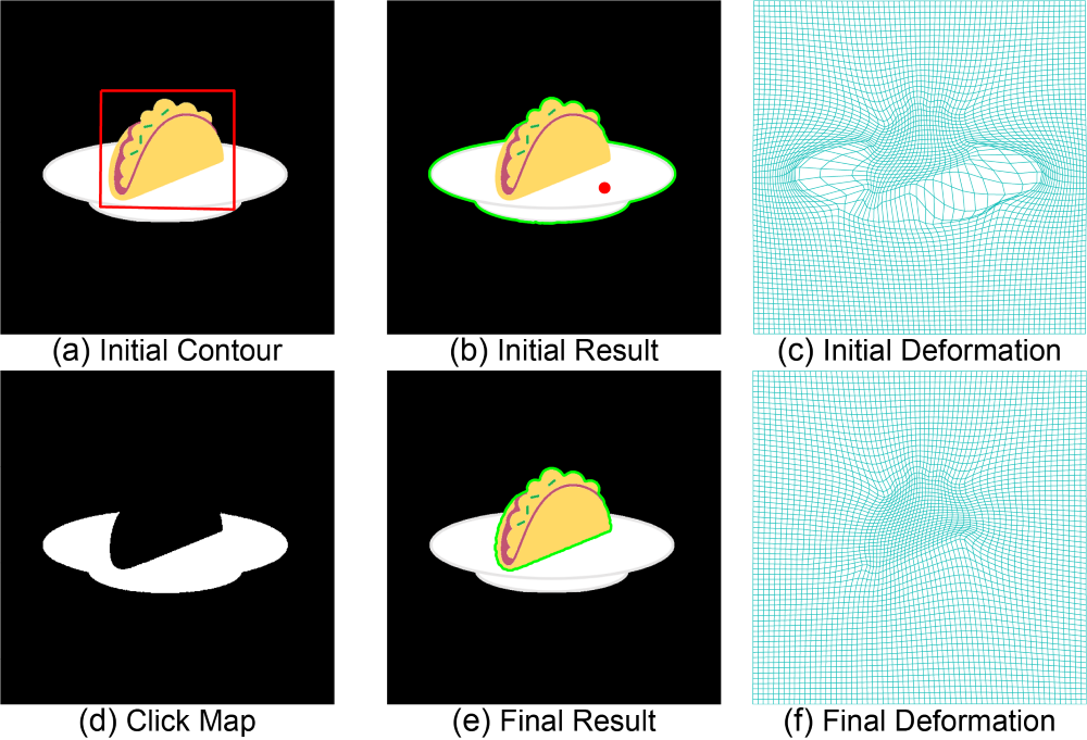
Figure 4: Segmentation result achieved by employing the QIS model on a synthesized image featuring a taco on a plate, with the objective of segmenting the taco.

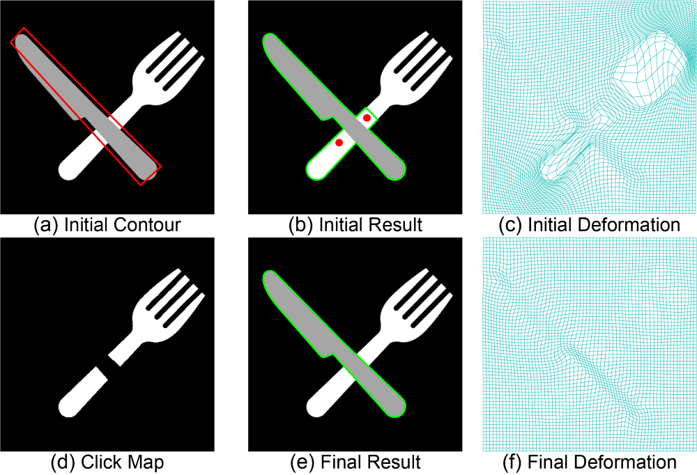
Figure 5: Segmentation result attained by utilizing the QIS model on a synthesized image highlighting the eating utensils, specifically the knife and fork, with the aim of segmenting the knife.

We first test our proposed model on simple synthetic images. Figure 4 illustrates the quasiconformal interactive segmentation of an image featuring a taco on a plate. Our goal is to segment the taco. The initial contour is a simple rectangle, as shown in (a). The initial contour defines the desired topology of the segmentation mask, which is simply-connected. The initial segmentation result using the quasiconformal segmentation model is displayed in (b), which includes the plate as well. The deformation $\phi$ that transforms the initial contour to the initial result is shown in (c). To exclude the plate from the segmentation mask, we introduce a negative click on the plate, represented by the red dot in (b). The click map associated with this click is shown in (d). The quasiconformal interactive segmentation result is presented in (e), accurately segmenting the desired taco. The deformation corresponding to the final interactive segmentation result is shown in (f), which is bijective. Thus, the segmentation mask preserves the same topology as the initial contour..

Figure 5 presents another synthetic image featuring two eating utensils: a fork and a knife. Our objective is to segment the knife. (a) shows the initial contour, which is a simple rectangle. Again, the initial contour defines the desired topology of the segmentation mask, which is simply-connected. The initial segmentation result using the quasiconformal segmentation model is displayed in (b), with its corresponding deformation shown in (c). Clearly, the segmentation mask includes some undesired regions. To exclude these undesired regions, two negative clicks are introduced, indicated by the red dots in (b). The click map associated with these clicks is shown in (d). The quasiconformal interactive segmentation result is presented in (e), accurately segmenting the desired knife. The deformation corresponding to the interactive segmentation result is shown in (f), which is bijective. Thus, the segmentation mask preserves the same topology as the initial contour.

7.2 Interactive segmentation of medical images

In this subsection, we evaluate our proposed segmentation model on real medical images. More specifically, we use brain magnetic resonance images (MRIs) from the BraTs21 dataset in our experiment.

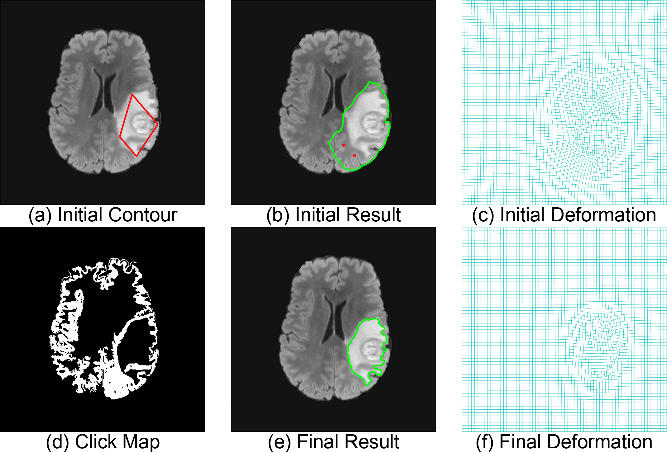
Figure 6: Segmentation result achieved by employing the QIS model on a brain MRI, with the goal of extracting the lesion region.

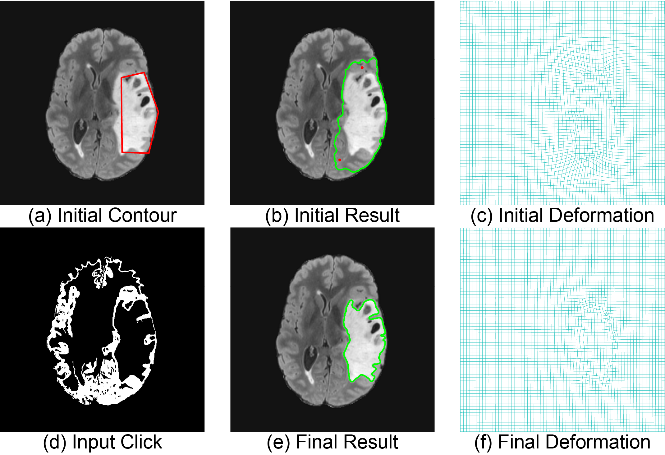
Figure 7: Another example of a segmentation result obtained by utilizing the QIS model on a different brain MRI, aiming to extract the lesion region.

Figure 6 shows an MRI of a brain with a lesion region. Our objective is to segment the lesion region. (a) presents the initial contour, which is a simply-connected polygon. (b) depicts the initial segmentation mask obtained using the quasiconformal segmentation model, and the corresponding deformation is shown in (c). Clearly, the segmentation mask contains some undesired regions that do not belong to the lesion region. To exclude these undesired regions, two negative clicks are introduced and indicated by the red dots in (b). (d) shows the corresponding click map. By employing our proposed QIS model, the segmentation result is presented in (e), accurately segmenting the lesion. The corresponding deformation is shown in (f), which is bijective. Thus, the segmentation mask preserves the same topology as the initial contour.

Figure 7 presents another example of interactively segmenting the lesion region of a brain MRI. The initial segmentation result with a simply-connected initial contour using the quasiconformal segmentation model is displayed in (b), and the corresponding deformation is shown in (c). Once again, the initial segmentation mask contains some undesired regions that do not belong to the lesion region. Two negative clicks, indicated as red dots in (b), are introduced to exclude these undesired regions. The click map is shown in (d). By incorporating the click map, the QIS model accurately segments the lesion region. The segmentation mask preserves the same topology as the initial contour, which is also evident from the bijective deformation shown in (f).

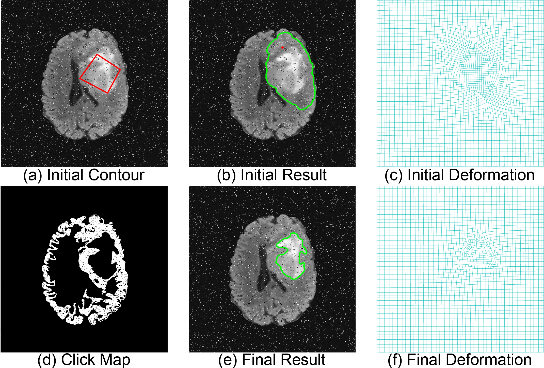
Figure 8: Segmentation result obtained by applying the proposed QIS model to extract the lesion region from a noisy brain MRI.

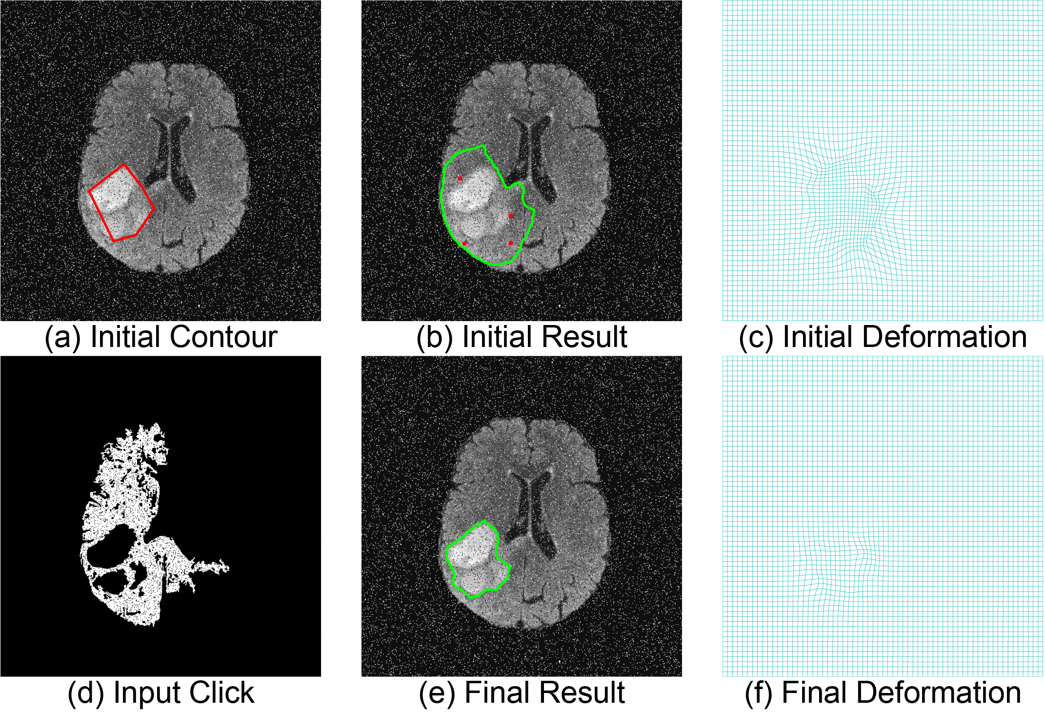
Figure 9: Another instance of a segmentation result obtained by applying the proposed QIS model to extract the lesion region from a different noisy brain MRI.

Figure 8 and Figure 9 show the results of QIS on two noisy brain MRIs, with the objective of extracting the lesion region. In each figure, (a) displays the initial contour, while the initial segmentation result using the quasiconformal segmentation model is shown in (b). The corresponding segmentation mask is displayed in (c). In both cases, the initial segmentation mask contains some undesired regions. To exclude these undesired regions, negative clicks are introduced, indicated by the red dots in (b). By incorporating the corresponding click map in (d), our proposed QIS model accurately segments the lesion region. The segmentation mask preserves the same topology as the initial contour, as evidenced by the bijective deformation shown in (f). These examples illustrate the effectiveness of our proposed QIS model, even on noisy images.

7.3 Comprehensive analysis of QIS model

In this subsection, we perform a more comprehensive analysis of our proposed QIS model.

Comparison with modified Chan-Vese segmentation model

The QIS model is a deformation-based segmentation model incorporating the quasiconformal segmentation model with the click map. One advantage of the quasiconformal segmentation model is that it ensures the segmentation mask maintains the prescribed topology, avoiding topological errors and enhancing the accuracy and efficiency of the interactive segmentation model. To investigate the importance of incorporating the quasiconformal segmentation model, we compare our method with an alternative method that integrates the level-set segmentation model with the click map. Instead of utilizing the quasiconformal segmentation model, we can run the Chan-Vese segmentation model with $I+rM_{clicks}$ as the input image using a suitable parameter $r$. The segmentation results of several natural images using the modified Chan-Vese model are presented in Figure 10. The first row of Figure 10 illustrates the initial segmentation outcomes of four natural images using the conventional Chan-Vese segmentation model. The two images on the left are clean, while the two on the right are noisy. The second row displays the initial segmentation results of the same four natural images using the quasiconformal segmentation model. In both methods, the initial segmentation masks include some undesired regions and exclude certain regions of interest. Some positive clicks (in blue) and negative clicks (in red) are introduced to guide the segmentation. The third row shows the segmentation results obtained by the modified Chan-Vese segmentation method, incorporating click maps. The segmentation masks exhibit improved accuracy in segmenting the regions of interest, though they are not entirely precise. Finally, the last row demonstrates the segmentation results obtained by the QIS model, which accurately segments the regions of interest. The topology of the segmentation mask is also consistent with that of the initial contour. Note that the clicks inputted by users are the same for both the modified Chan-Vese segmentation model and the QIS model.

Figure 11 presents another comparison using brain MRIs. The first row of Figure 11 shows the initial segmentation results of four brain MRIs using the conventional Chan-Vese segmentation model. Again, the two images on the left are clean, while the two on the right are noisy. Evidently, the initial segmentation masks contain some undesired regions and exclude some regions of interest. The second row shows the segmentation results obtained by the modified Chan-Vese segmentation method, incorporating click maps. The clicks inputted by the users are the same as those used by the QIS model, as shown in Figure 6, Figure 7, Figure 8 and Figure 9. The segmentation masks can better segment the lesion, although they are still not accurate. The last row shows the segmentation results obtained by the QIS model, which accurately segments the lesions. The topology of the segmentation mask is consistent with that of the initial contour.

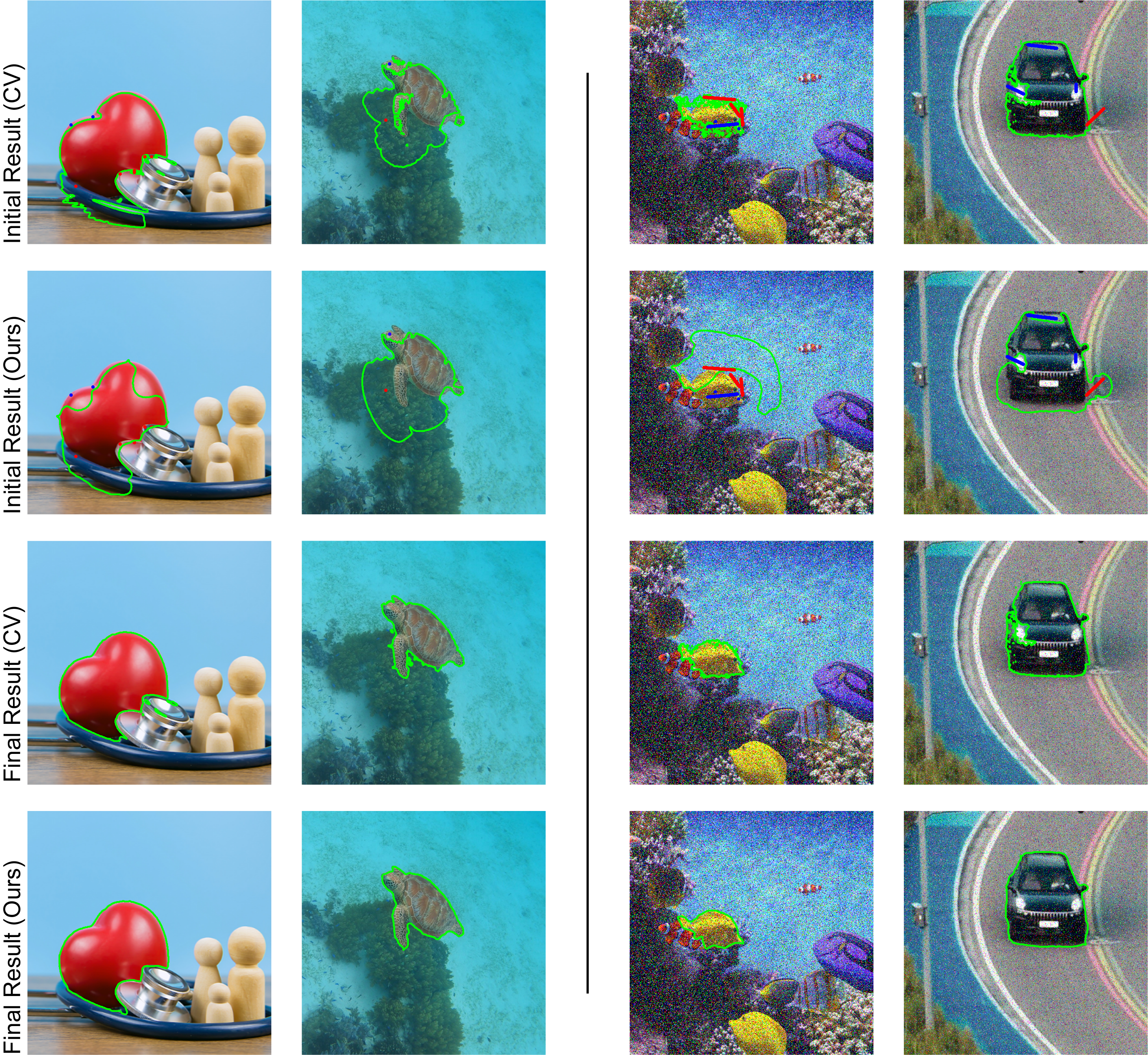
Figure 10: Segmentation results on natural images obtained using the QIS model and the modified Chan-Vese segmentation model with the integration of click maps. The left side displays the segmentation results on two clean images, while the right side shows the segmentation results on two noisy images.

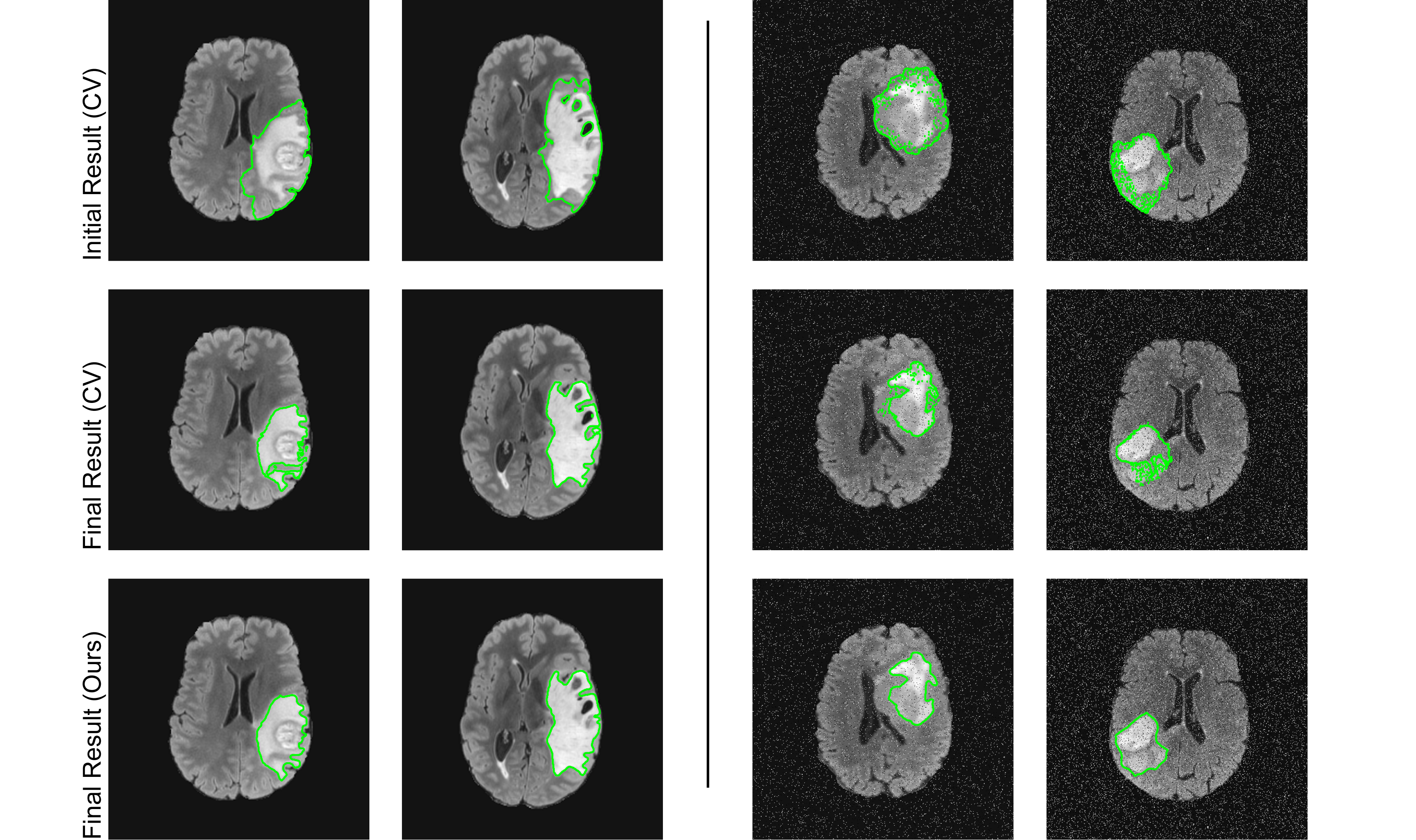
Figure 11: Segmentation results on brain MRIs obtained using the QIS model and the modified Chan-Vese segmentation model with the integration of the click map. The left side displays the segmentation results on two clean brain MRIs, while the right side shows the segmentation results on two noisy brain MRIs.

Comparison with GrabCut

We compare the QIS model with a popular interactive segmentation model called GrabCut. Similar to the QIS model, GrabCut requires the user to provide interactive inputs of foreground and background brushes. The comparison between the QIS and GrabCut methods on a noisy image capturing flowers is shown in Figure 12. In Figure 12(a), the iterative process of the QIS model is displayed. The negative clicks in each iteration, represented by red brushes, are also shown. The QIS effectively segments the noisy image in four steps with only a few brushes introduced. Figure 12(b) illustrates the iterative process of GrabCut, where the brushes introduced by the user (red for foreground and blue for background) are also shown. GrabCut produces a reasonably accurate segmentation mask after seven steps, although it is evident that it is comparatively less accurate than QIS. Figure 13 shows a further comparison between GrabCut and QIS using another noisy image capturing a road scene, with the objective of segmenting the car. The iterative process of QIS is shown in (a), where the positive and negative clicks are denoted by red and blue brushes respectively. QIS accurately segments the car in just five steps. (b) displays the iterative process using GrabCut, with the segmentation result after eight steps exhibited, which is comparatively less accurate than QIS.

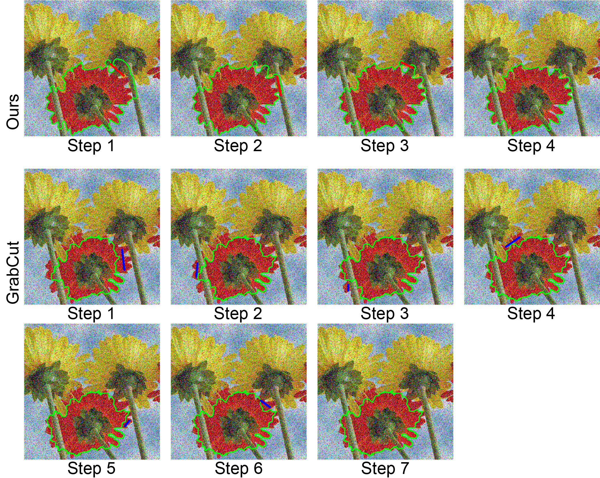
Figure 12: Comparison between QIS and GrabCut segmentation methods. The top shows the iterative segmentation process using the QIS method, with negative clicks labeled in red brushes. The final segmentation result is obtained in 4 steps. The bottom shows the iterative process using the GrabCut method, with positive and negative brushes labeled in blue and red, respectively. The segmentation result after 7 steps is displayed.

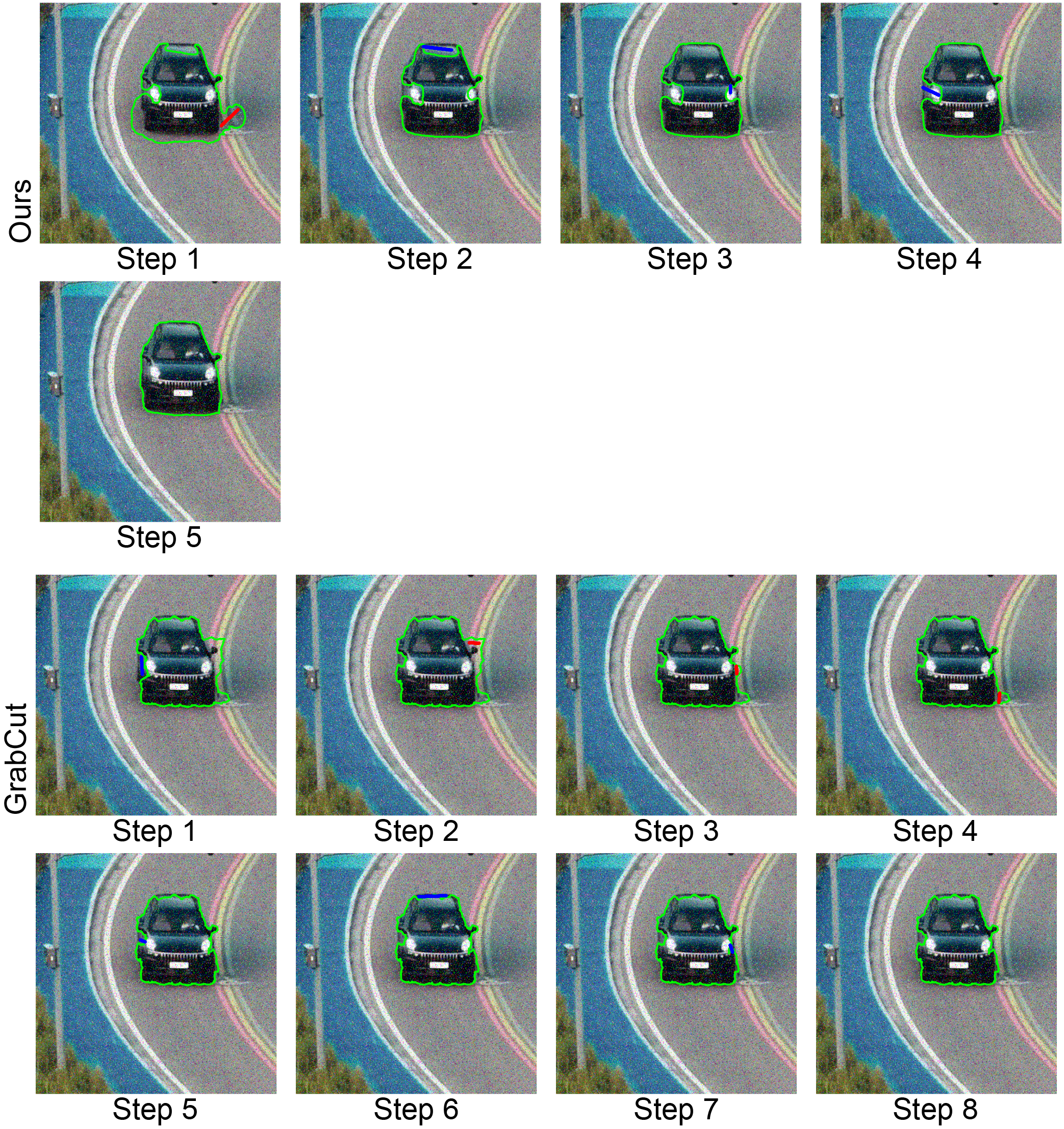
Figure 13: Another comparison between the QIS and GrabCut segmentation methods. The top demonstrates the iterative segmentation process using the QIS method, with positive and negative clicks labeled as blue and red brushes respectively. The final segmentation result is achieved in 5 steps. The bottom depicts the iterative process using the GrabCut method, with positive and negative brushes labeled as blue and red respectively. The segmentation result after 8 steps is displayed.

Robustness across varied click choices

The QIS model relies on user inputs, specifically the positioning of positive and negative clicks. It is essential to examine the robustness of the QIS model when subjected to different click choices. Figure 14 depicts the robustness of the QIS model under various click choices. The initial segmentation mask contains undesired regions. In order to exclude these regions, different negative click options are introduced, as illustrated in the first row. The corresponding segmentation results produced by the QIS model, utilizing different click choices, are displayed in the second row. It is evident that the segmentation results remain consistent across different click choices, accurately delineating the lesion region. This exemplifies the robustness of the QIS model under different click choices.

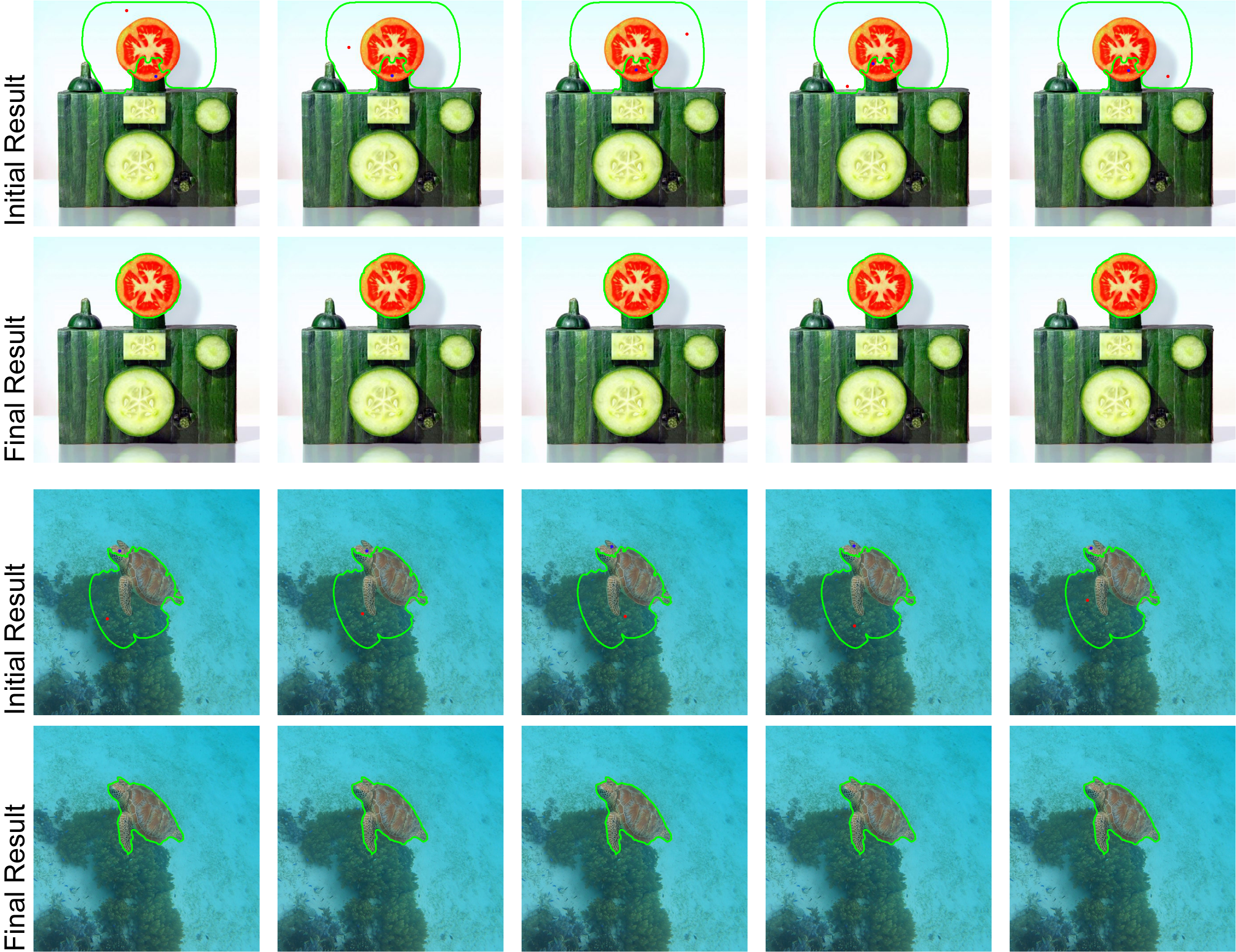
Figure 14: Segmentation results for extracting the region of interest obtained by the QIS model using different click choices. In each case, the upper row displays the initial segmentation results and input click positions, while the lower row presents the corresponding final segmentation results.

8 Conclusion

In this paper, we propose the quasi-conformal interactive segmentation (QIS) model, with the incorporation of user’s interactions. User’s interactions are defined by two actions: a positive click and a negative click, represented by left and right clicks, respectively. These clicks serve to indicate the regions that the user wants to include or exclude from the segmentation process. Clicks are transformed into a click map, which is then integrated into the proposed model using a novel interactive segmentation energy term that we have designed. The segmentation mask is obtained by deforming a template mask with the same topology as the object of interest using an orientation-preserving quasiconformal mapping. This approach helps to avoid topological errors in the segmentation results. We provide a thorough analysis of the proposed model, including theoretical support for the ability of QIS to include or exclude regions of interest or disinterest based on the user’s indication. To evaluate the performance of QIS, we conduct experiments on synthesized images, medical images, natural images, and noisy natural images. The results demonstrate the efficacy of our proposed method.

Looking ahead, there are two key directions for future work. First, we aim to extend the QIS model to 3D image segmentation, enabling its application in volumetric data. Second, we plan to enhance segmentation outcomes by incorporating edge-aware energies, which can further improve the accuracy and robustness of the QIS model in challenging imaging scenarios.

References

- [1] H. Ali, S. Faisal, K. Chen, and L. Rada, Image-selective segmentation model for multi-regions within the object of interest with application to medical disease, The Visual Computer, 37 (2021), pp. 939–955.
- [2] L. Bers, Quasiconformal mappings, with applications to differential equations, function theory and topology, Bulletin of the American Mathematical Society, 83 (1977), pp. 1083–1100.
- [3] C. Broit, Optimal Registration of Deformed Images, PhD thesis, University of Pennsylvania, USA, 1981.
- [4] H.-L. Chan, S. Yan, L.-M. Lui, and X.-C. Tai, Topology-preserving image segmentation by beltrami representation of shapes, Journal of Mathematical Imaging and Vision, 60 (2018), pp. 401–421.
- [5] D. Chen, J. Spencer, J.-M. Mirebeau, K. Chen, M. Shu, and L. D. Cohen, A generalized asymmetric dual-front model for active contours and image segmentation, IEEE Transactions on Image Processing, 30 (2021), pp. 5056–5071.
- [6] X. Chen, Z. Zhao, F. Yu, Y. Zhang, and M. Duan, Conditional diffusion for interactive segmentation, in Proc. of Int. Conf. on Computer Vision, 2021, pp. 7345–7354.
- [7] X. Chen, Z. Zhao, Y. Zhang, M. Duan, D. Qi, and H. Zhao, Focalclick: towards practical interactive image segmentation, in Proc. of IEEE/CVF Conf. on Computer Vision & Pattern Recognition, 2022, pp. 1300–1309.
- [8] G. P. T. Choi, K. T. Ho, and L. M. Lui, Spherical conformal parameterization of genus-0 point clouds for meshing, SIAM Journal on Imaging Sciences, 9 (2016), pp. 1582–1618.
- [9] G. P. T. Choi, Y. Liu, and L. M. Lui, Free-boundary conformal parameterization of point clouds, Journal of Scientific Computing, 90 (2022), pp. 1–26.
- [10] P. T. Choi and L. M. Lui, Fast disk conformal parameterization of simply-connected open surfaces, Journal of Scientific Computing, 65 (2015), pp. 1065–1090.
- [11] N. Chumchob, K. Chen, and C. Brito, A fourth-order variational image registration model and its fast multigrid algorithm, Multiscale Modeling & Simulation, 9 (2011), pp. 89–128.
- [12] T. F. Cootes, C. J. Taylor, D. H. Cooper, and J. Graham, Active shape models-their training and application, Computer Vision and Image Understanding, 61 (1995), pp. 38–59.
- [13] K. Crane, U. Pinkall, and P. Schröder, Robust fairing via conformal curvature flow, ACM Trans. on Graphics, 32 (2013), pp. 1–10.
- [14] B. Fischer and J. Modersitzki, Curvature based image registration, Journal of Mathematical Imaging and Vision, 18 (2003), pp. 81–85.
- [15] B. Fischer and J. Modersitzki, A unified approach to fast image registration and a new curvature based registration technique, Linear Algebra and Its Applications, 380 (2004), pp. 107–124.
- [16] F. P. Gardiner and N. Lakic, Quasiconformal teichmuller theory, vol. 76, American Mathematical Soc., 2000.
- [17] L. Grady, Random walks for image segmentation, IEEE Transactions on Pattern Analysis and Machine Intelligence, 28 (2006), pp. 1768–1783.
- [18] X. Gu, Y. Wang, T. F. Chan, P. M. Thompson, and S.-T. Yau, Genus zero surface conformal mapping and its application to brain surface mapping, IEEE Transactions on Medical Imaging, 23 (2004), pp. 949–958.
- [19] X. Gu and S.-T. Yau, Global conformal surface parameterization, in Proceedings of the 2003 Eurographics/ACM SIGGRAPH symposium on Geometry processing, Eurographics Association, 2003, pp. 127–137.
- [20] V. Gulshan, C. Rother, A. Criminisi, A. Blake, and A. Zisserman, Geodesic star convexity for interactive image segmentation, in Proc. of IEEE/CVF Conf. on Computer Vision & Pattern Recognition, IEEE, 2010, pp. 3129–3136.
- [21] M. Ibrahim, K. Chen, and C. Brito-Loeza, A novel variational model for image registration using gaussian curvature, Geometry, Imaging and Computing, 1 (2014), pp. 417–446.
- [22] M. Jaderberg, K. Simonyan, A. Zisserman, et al., Spatial transformer networks, Proc. of Int. Conf. on Neural Information Processing Systems, 28 (2015).
- [23] W.-D. Jang and C.-S. Kim, Interactive image segmentation via backpropagating refinement scheme, in Proc. of IEEE/CVF Conf. on Computer Vision & Pattern Recognition, 2019, pp. 5297–5306.
- [24] M. Kass, A. Witkin, and D. Terzopoulos, Snakes: Active contour models, Int. J. of Computer Vision., 1 (1988), pp. 321–331.
- [25] T. H. Kim, K. M. Lee, and S. U. Lee, Nonparametric higher-order learning for interactive segmentation, in Proc. of IEEE/CVF Conf. on Computer Vision & Pattern Recognition, IEEE, 2010, pp. 3201–3208.
- [26] K. C. Lam and L. M. Lui, Landmark-and intensity-based registration with large deformations via quasiconformal maps, SIAM Journal on Imaging Sciences, 7 (2014), pp. 2364–2392.
- [27] S. Lang, Calculus of several variables, Springer Science & Business Media, 2012.
- [28] M. C. H. Lee, K. Petersen, N. Pawlowski, B. Glocker, and M. Schaap, Tetris: Template transformer networks for image segmentation with shape priors, IEEE Transactions on Medical Imaging, 38 (2019), pp. 2596–2606.
- [29] O. Lehto and K. I. Virtanen, Quasiconformal mappings in the plane, vol. 126, Citeseer, 1973.
- [30] B. Lévy, S. Petitjean, N. Ray, and J. Maillot, Least squares conformal maps for automatic texture atlas generation, ACM Trans. on Graphics, 21 (2002), pp. 362–371.
- [31] Z. Li, Q. Chen, and V. Koltun, Interactive image segmentation with latent diversity, in Proc. of IEEE/CVF Conf. on Computer Vision & Pattern Recognition, 2018, pp. 577–585.
- [32] J. H. Liew, S. Cohen, B. Price, L. Mai, S.-H. Ong, and J. Feng, Multiseg: Semantically meaningful, scale-diverse segmentations from minimal user input, in Proc. of Int. Conf. on Computer Vision, 2019, pp. 662–670.
- [33] Z. Lin, Z. Zhang, L.-Z. Chen, M.-M. Cheng, and S.-P. Lu, Interactive image segmentation with first click attention, in Proc. of IEEE/CVF Conf. on Computer Vision & Pattern Recognition, 2020, pp. 13339–13348.
- [34] L. M. Lui, K. C. Lam, S.-T. Yau, and X. Gu, Teichmuller mapping (t-map) and its applications to landmark matching registration, SIAM Journal on Imaging Sciences, 7 (2014), pp. 391–426.
- [35] D. B. Mumford and J. Shah, Optimal approximations by piecewise smooth functions and associated variational problems, Communications on Pure and Applied Mathematics, 42 (1989), pp. 577–685.
- [36] J. Panetta, M. Konaković-Luković, F. Isvoranu, E. Bouleau, and M. Pauly, X-shells: A new class of deployable beam structures, ACM Trans. on Graphics, 38 (2019), pp. 1–15.
- [37] L. Rada and K. Chen, A new variational model with dual level set functions for selective segmentation, Communications in Computational Physics, 12 (2012), pp. 261–283.
- [38] L. Rada and K. Chen, A variational model and its numerical solution for local, selective and automatic segmentation, Numerical Algorithms, 66 (2014), pp. 399–430.
- [39] R. Remmert, Theory of complex functions, vol. 122, Springer Science & Business Media, 1991.
- [40] M. Roberts, K. Chen, and K. L. Irion, A convex geodesic selective model for image segmentation, Journal of Mathematical Imaging and Vision, 61 (2019), pp. 482–503.
- [41] M. Roberts, K. Chen, and K. L. Irion, Multigrid algorithm based on hybrid smoothers for variational and selective segmentation models, International Journal of Computer Mathematics, 96 (2019), pp. 1623–1647.
- [42] C. Rother, V. Kolmogorov, and A. Blake, "grabcut" interactive foreground extraction using iterated graph cuts, ACM Trans. on Graphics, 23 (2004), pp. 309–314.
- [43] C. Y. Siu, H. L. Chan, and M. L. Lui, Image segmentation with partial convexity shape prior using discrete conformality structures, SIAM Journal on Imaging Sciences, 13 (2020), pp. 2105–2139.
- [44] K. Sofiiuk, I. Petrov, O. Barinova, and A. Konushin, f-brs: Rethinking backpropagating refinement for interactive segmentation, in Proc. of IEEE/CVF Conf. on Computer Vision & Pattern Recognition, 2020, pp. 8623–8632.
- [45] K. Sofiiuk, I. A. Petrov, and A. Konushin, Reviving iterative training with mask guidance for interactive segmentation, in Proc. of IEEE Int. Conf. on Image Processing, 2022, pp. 3141–3145.
- [46] Y. Soliman, D. Slepčev, and K. Crane, Optimal cone singularities for conformal flattening, ACM Trans. on Graphics, 37 (2018), pp. 1–17.
- [47] J. Spencer and K. Chen, A convex and selective variational model for image segmentation, Communications in Mathematical Sciences, 13 (2015), pp. 1453–1472.
- [48] J. Spencer, K. Chen, and J. Duan, Parameter-free selective segmentation with convex variational methods, IEEE Transactions on Image Processing, 28 (2018), pp. 2163–2172.
- [49] N. Xu, B. Price, S. Cohen, J. Yang, and T. S. Huang, Deep interactive object selection, in Proc. of IEEE/CVF Conf. on Computer Vision & Pattern Recognition, 2016, pp. 373–381.
- [50] D. Zhang and K. Chen, A novel diffeomorphic model for image registration and its algorithm, Journal of Mathematical Imaging and Vision, 60 (2018), pp. 1261–1283.
- [51] D. Zhang, G. P. T. Choi, J. Zhang, and L. M. Lui, A unifying framework for n-dimensional quasi-conformal mappings, SIAM Journal on Imaging Sciences, 15 (2022), pp. 960–988.
- [52] D. Zhang and L. M. Lui, Topology-preserving 3d image segmentation based on hyperelastic regularization, Journal of Scientific Computing, 87 (2021), pp. 1–33.
- [53] D. Zhang, X.-C. Tai, and L. M. Lui, Topology-and convexity-preserving image segmentation based on image registration, Applied Mathematical Modelling, 100 (2021), pp. 218–239.
- [54] H. Zhang and L. M. Lui, Topology-preserving segmentation network: A deep learning segmentation framework for connected component, arXiv preprint arXiv:2202.13331, (2022).
- [55] J. Zhang and K. Chen, Variational image registration by a total fractional-order variation model, Journal of Computational Physics, 293 (2015), pp. 442–461.