On Schrödingerization based quantum algorithms for linear dynamical systems with inhomogeneous terms

Abstract

We analyze the Schrödingerisation method for quantum simulation of a general class of non-unitary dynamics with inhomogeneous source terms. The Schrödingerisation technique, introduced in [26, 28], transforms any linear ordinary and partial differential equations with non-unitary dynamics into a system under unitary dynamics via a warped phase transition that maps the equations into a higher dimension, making them suitable for quantum simulation. This technique can also be applied to these equations with inhomogeneous terms modeling source or forcing terms or boundary and interface conditions, and discrete dynamical systems such as iterative methods in numerical linear algebra, through extra equations in the system. Difficulty airses with the presense of inhomogeneous terms since it can change the stability of the original system.

In this paper, we systematically study–both theoretically and numerically–the important issue of recovering the original variables from the Schrödingerized equations, even when the evolution operator contains unstable modes. We show that even with unstable modes, one can still construct a stable scheme, yet to recover the original variable one needs to use suitable data in the extended space. We analyze and compare both the discrete and continuous Fourier transforms used in the extended dimension, and derive corresponding error estimates, which allows one to use the more appropriate transform for specific equations. We also provide a smoother initialization for the Schrodödingerized system to gain higher order accuracy in the extended space. We homogenize the inhomogeneous terms with a stretch transformation, making it easier to recover the original variable. Our recovering technique also provides a simple and generic framework to solve general ill-posed problems in a computationally stable way.

Keywords: quantum algorithms, Schrödingerisation, non-unitary dynamics, differential equations with inhomogeneous terms

1 Introduction

Quantum computing is considered a promising candidate to overcome many limitations of classical computing [17, 36, 37], one of which is the curse-of-dimensionality. It has been shown that quantum computers could potentially outperform the most powerful classical computers, with polynomial or even exponential speed-up, for certain types of problems [18, 32].

In this paper, we concentrate on the general linear dynamical system as follows

$$\frac{\mathrm{d}}{\mathrm{d}t}{\bm{u}}=A(t){\bm{u}}(t)+{\bm{b}}(t),\quad{\bm{u}}(0)={\bm{u}}_{0},$$ (1.1)

where ${\bm{u}}$, ${\bm{b}}\in\mathbb{C}^{n}$, $A\in\mathbb{C}^{n\times n}$ is a time-dependent matrix. This system includes ordinary differential equations (ODEs), and partial differential equations (PDEs) (for continous representation, in which case $A(t)$ is the differential operator, as well as spatially discrete version, in which a PDE becomes a system of ODEs). Classical algorithms become inefficient or even prohibitively expensive due to large dimension $n$ whereas quantum methods can possibly significantly speed up the computation. Therefore, the design for quantum simulation algorithms for solving general dynamical systems–including both ODEs and PDEs–is important for a wide range of applications, for examples molecular dynamics simulations, and high dimensional and multi-scale PDEs.

The development of quantum algorithms with up to exponential advantage excel in unitary dynamics, in which $A(t)=iH(t)$ with $H=H^{\dagger}$ (where $\dagger$ represents complex conjugate) and ${\bm{b}}=\textbf{0}$ in (1.1), which is also known as the Hamiltonian simulation. Many efficient quantum algorithms for Hamiltonian simulation have been developed in the literature, for example [5, 7, 8, 9, 31, 34, 10, 2, 3, 6, 11, 16, 14, 1]. However, most dynamical systems in applications involve non-unitary dynamics which make them unsuitable for quantum simulation. A very recent proposal for such problems is based on Schrödingerisation, which converts non-unitary dynamics to systems of Schr$\ddot{\text{o}}$dinger type equations with unitary dynamics by a warped phase transformation that maps the system to one higher dimension, while the original variable ${\bm{u}}$ can be recovered via integration or pointwise evaluation of the variable in the extra dimensional space. This technique can be applied in both qubits [26, 28] and continuous-variable frameworks [22], the latter suitable for analog quantum computing. The method can also be extended to solve open quantum systems in a bounded domain with artificial boundary conditions [24], physical and interface conditions [21], and even discrete dynamical systems such as iterative methods in numerical linear algebra [29].

For non-Hermitian $H(t)$, the Schrödingerizaiton first decomposes it into the Hermitian and anti-Hermitian parts:

$$A=H_{1}+H_{2},\qquad H_{1}=(A+A^{\dagger})/2,\qquad H_{2}=(A-A^{\dagger})/(2i),$$ (1.2)

where $H_{1}=H_{1}^{\dagger},H_{2}=H_{2}^{\dagger}$, followed by the warped phase transformation for the $H_{1}$ part. A basic assumption for the application of the Schrödingerization technique is that the eigenvalues of $H_{1}$ need to be negative [26, 28]. This corresponds to the stability of solution to the original system (1.1). When there is an inhomogeneous term $b(t)$, one needs to enlarge the system so as to deal with just a homogeneous system. However, the new $H_{1}$ corresponding to the enlarged system will have positive eigenvalues–which will be proved in this paper– violating the basic assumption of the Schrödingerization method. We address this important issue in this paper.

We show that even if some of the eigenvalues of $H_{1}$ are positive, the Schrödingerization method can still be applied. However, in this case one needs to be more careful when recovering the original variable ${\bm{u}}$. Specifically, one can still obtain ${\bm{u}}$ by using an appropriate domain in the new extended space, which is not ‘distorted’ by spurious right-moving waves generated by the positive eigenvalues of $H_{1}$.

We will also analyze both discrete and continuous Fourier transformations used in the extended dimension. The corresponding error estimates for the discretization will be established. A smoothed initializtion is also introduced to provide a higher order accuracy in approximations in the extended dimension (see Remark 4.1). Furthermore, a stretching transformation is used to lower the impact of positive eigenvalues of $H_{1}$, which makes it easier to recover the original variables. We also show that the stretch coefficient does not affect the error of the Schrödingerisation discretization.

The rest of the paper is organized as follows. In section 2, we give a brief review of the Schrödingerisation approach for general homogeneous linear ODEs and two different Fourier discretizations in the extended space for this problem. In section 3, we show the conditions for correct recovery from the warped transformation, even when there exist positive eigenvalues of $H_{1}$, which triggers potential instability for the extended dynamical system. We also show the implementation protocol on quantum devices. The error estimates are established in section 4. In section 5, we consider the inhomogeneous problems and show that the enlarged homogeneous system will contain unstable modes corresponding to positive eigenvalues of $H_{1}$. The recovering technique introduced in Section 3 can be used to deal with this system. Finally, we show the numerical tests in section 6.

Throughout the paper, we restrict the simulation to a finite time interval $t\in[0,T]$. The notation $f\lesssim g$ stands for $f\leq Cg$ where $C$ is a positive constant independent of the numerical mesh size and time step. Moreover, we use a 0-based indexing, i.e. $j=\{0,1,\cdots,N-1\}$, or $j\in[N]$, and $|j\rangle\in\mathbb{C}^{N}$, to denote a vector with the $j$-th component being $1$ and others $0$. We shall denote the identity matrix and null matrix by $I$ and 0, respectively, and the dimensions of these matrices should be clear from the context, otherwise, the notation $I_{N}$ stands for the $N$-dimensional identity matrix. Without specific statement, $\|{\bm{b}}\|$ denotes the Euclidean norm defined by $\|{\bm{b}}\|=(\sum_{i}|b_{i}|^{2})^{1/2}$ and $\|A\|$ denotes matrix $2-$norms defined by $\|A\|=\sup_{\|{\bm{x}}\|=1}\|A{\bm{x}}\|$. The vector-valued quantities are denoted by boldface symbols, such as ${\bm{L}}^{2}(I)=(L^{2}(I))^{n}$.

2 A review of Schrödingerisation for general linear dynamical systems

In this section, we briefly review the Schr$\ddot{\text{o}}$dingerisation approach for general linear dynamical systems. Defining an auxiliary vector function ${\bm{r}}(t)\equiv\sum_{i}|i\rangle\in\mathbb{R}^{n}$ that remains constant in time, system (1.1) can be rewritten as a homogeneous system

$$\frac{\mathrm{d}}{\mathrm{d}t}\begin{bmatrix}{\bm{u}}\\ {\bm{r}}\end{bmatrix}=\begin{bmatrix}A&B\\ \textbf{0}&\textbf{0}\end{bmatrix}\begin{bmatrix}{\bm{u}}\\ {\bm{r}}\end{bmatrix},\qquad\begin{bmatrix}{\bm{u}}(0)\\ {\bm{r}}(0)\end{bmatrix}=\begin{bmatrix}{\bm{u}}_{0}\\ {\bm{r}}_{0}\end{bmatrix},$$ (2.1)

where $B=\text{diag}\{b_{1},b_{2},\cdots,b_{n}\}$ and ${\bm{r}}_{0}=\sum_{i}|i\rangle\in\mathbb{R}^{n}$. Therefore, without loss of generality, we assume ${\bm{b}}=\textbf{0}$ in (1.1). Since any matrix can be decomposed into a Hermitian term and an anti-Hermitian one as in (1.2), Equation (1.1) can be expressed as

$$\frac{\mathrm{d}}{\mathrm{d}t}{\bm{u}}=H_{1}{\bm{u}}+iH_{2}{\bm{u}},\quad{\bm{u}}(0)={\bm{u}}_{0}.$$ (2.2)

The Schrödingerization method [26, 27] assumes that all eigenvalues of $H_{1}$ are negative. This corresponds to assuming that the original dynamical system (1.1) is stable. Using the warped phase transformation ${\bm{w}}(t,p)=e^{-p}{\bm{u}}$ for $p>0$ and symmetrically extending the initial data to $p<0$, Equation (2.2) is converted to a system of linear convection equations:

$$\frac{\mathrm{d}}{\mathrm{d}t}{\bm{w}}=-H_{1}\partial_{p}{\bm{w}}+iH_{2}{\bm{w}},\quad{\bm{w}}(0)=e^{-|p|}{\bm{u}}_{0}.$$ (2.3)

When the eigenvalues of $H_{1}$ are all negative, the convection term of (2.3) corresponds to a wave moving from the right to the left, thus one does not need to impose a boundary condition for ${\bm{w}}$ at $p=0$. One does, however, need a boundary condition on the right hand side. Since ${\bm{w}}$ decays exponentially in $p$, one just needs to select $p=p^{*}$ large enough, so $w$ at this point is essentially zero and a zero incoming boundary condition can be used at $p=p^{*}$. Then ${\bm{u}}$ can be recovered via

$${\bm{u}}(t)=\int_{0}^{p^{*}}w(t,p)\,dp$$

or

$${\bm{u}}(t)=e^{p}w(t,p)\qquad{\text{ for any}}\quad 0<p<p^{*}.$$

2.1 The discrete Fourier transform for Schrödingerisation

To discretize the $p$ domain, we choose a large enough domain $p\in[-\pi L,\pi L]$ and set the uniform mesh size $\triangle p=2\pi L/N$ where $N$ is a positive even integer and the grid points are denoted by $-\pi L=p_{0}<\cdots<p_{N}=\pi L$. Define the vector ${\bm{w}}_{h}$ the collection of the function ${\bm{w}}$ at these grid points by

$${\bm{w}}_{h}=\sum_{k\in[N]}\sum_{j\in[n]}w_{j}(t,p_{k})|k\rangle|j\rangle.$$ (2.4)

where $w_{j}$ is the $j$-th component of ${\bm{w}}$. The $1$-D basis functions for the Fourier spectral method are usually chosen as

$$\phi_{l}(p)=e^{i\mu_{l}(p+\pi L)},\qquad\mu_{l}=(l-N/2)/L,\quad l\in[N].$$ (2.5)

Using (2.5), we define

$$\Phi=(\phi_{jl})_{N\times N}=(\phi_{l}(p_{j}))_{N\times N},\quad D_{p}=\text{diag}\{\mu_{0},\cdots,\mu_{N-1}\}.$$ (2.6)

Considering the Fourier spectral discretisation on $p$, one easily gets

$$\frac{\mathrm{d}}{\mathrm{d}t}{\bm{w}}_{h}=-i(P\otimes H_{1}){\bm{w}}_{h}+i(I_{N}\otimes H_{2}){\bm{w}}_{h}.$$ (2.7)

Here $P$ is the matrix representation of the momentum operator $-i\partial_{p}$ and defined by $P=\Phi D_{p}\Phi^{-1}$. Through a change of variables $\tilde{{\bm{w}}}_{h}=[\Phi^{-1}\otimes I_{n}]{\bm{w}}_{h}$, one gets

$$\begin{cases}\frac{\mathrm{d}}{\mathrm{d}t}\tilde{{\bm{w}}}_{h}=-i[(D_{p}\otimes H_{1})-(I_{N}\otimes H_{2})]\tilde{{\bm{w}}}_{h}=-iH^{d}\tilde{{\bm{w}}}_{h},\\ \tilde{\bm{w}}_{h}(0)=[\Phi^{-1}\otimes I_{n}]{\bm{w}}_{h}(0).\end{cases}$$ (2.8)

At this point, a quantum algorithm for Hamiltonian simulation can be constructed for the above linear system (2.8). If $H_{1}$ and $H_{2}$ are usually sparse, then the Hamiltonian $H=D_{p}\otimes H_{1}-I_{N}\otimes H_{2}$ inherits the sparsity. The approximation of ${\bm{w}}$ is defined by

$${\bm{w}}_{h}^{d}=\sum_{|k|\leq N/2}\tilde{\bm{w}}_{j_{k}}e^{ik(p/L+\pi)},\quad j_{k}=k+N/2,$$ (2.9)

where $\tilde{\bm{w}}_{j_{N/2}}=\tilde{\bm{w}}_{j_{-N/2}}$ and $\tilde{\bm{w}}_{j_{k}}=(E_{j_{k}}\otimes I_{n})\tilde{\bm{w}}_{h}$ with $E_{j_{k}}=\text{diag}(|j_{k}\rangle)\in\mathbb{R}^{N,N}$.

2.2 The continuous Fourier transform for Schrödingerisation

In the previous section, $\partial_{p}w(t,p)$ is first discretized in $p$ by the discrete Fourier transform. Here, we consider the continuous Fourier transform of ${\bm{w}}(p)$ and its inverse transformation defined by

$$\hat{{\bm{w}}}:=\mathscr{F}({\bm{w}})(\xi)=\frac{1}{2\pi}\int_{\mathbb{R}}e^{i\xi p}{\bm{w}}(p)\,\mathrm{d}p,\qquad{\bm{w}}:=\mathscr{F}^{-1}(\hat{\bm{w}})(p)=\int_{\mathbb{R}}e^{-i\xi p}\hat{{\bm{w}}}(\xi)\mathrm{d}\xi.$$ (2.10)

The continuous Fourier transform in $p$ for (2.3) gives

$$\frac{\mathrm{d}}{\mathrm{d}t}\hat{{\bm{w}}} =i\xi H_{1}\hat{{\bm{w}}}+iH_{2}\hat{{\bm{w}}}=i(\xi H_{1}+H_{2})\hat{{\bm{w}}},$$ (2.11)

$$\hat{{\bm{w}}}(0) =\frac{1}{\pi(1+\xi^{2})}{\bm{u}}_{0}.$$

We can first consider the truncation of the $\xi$- domain to a finite interval $[-X,X]$. Then canonical Hamiltonian simulation methods can be applied to the following unitary dynamics

$$\begin{cases}\frac{\mathrm{d}}{\mathrm{d}t}\check{{\bm{w}}}_{h}=i(D_{\xi}\otimes H_{1}+I_{N+1}\otimes H_{2})\check{{\bm{w}}}_{h}=iH^{c}\check{{\bm{w}}}_{h},\\ \check{{\bm{w}}}_{h}(0)=\bm{\xi}_{h}\otimes{\bm{u}}_{0},\end{cases}$$ (2.12)

where $D_{\xi}=\text{diag}\{\xi_{0},\xi_{1},\cdots,\xi_{N}\}$ and $\bm{\xi}_{h}=\sum\limits_{j=0}^{N}\frac{|j\rangle}{\pi(1+\xi_{j}^{2})}$. The approximation for ${\bm{w}}$ is computed by

$${\bm{w}}_{h}^{c}=\triangle\xi\sum_{j=1}^{N-1}\check{\bm{w}}_{j}e^{-i\xi_{j}p}+\frac{\triangle\xi}{2}\big{(}\check{\bm{w}}_{N}e^{-i\xi_{N}p}+\check{\bm{w}}_{0}e^{-i\xi_{0}p}\big{)}.$$ (2.13)

Here $\check{\bm{w}}_{j}=(E_{j}\otimes I_{n})\check{\bm{w}}_{h}$ with $E_{j}=\text{diag}(|j\rangle)\in\mathbb{R}^{N+1,N+1}$. Without considering the error of quantum simulation, one gets $\check{\bm{w}}_{j}=\check{\bm{w}}_{h}(t,\xi_{j})$, $\xi_{j}=-X+2Xj/N$. It is obvious to see that ${\bm{w}}_{h}^{c}$ is the numerical integration of $\int_{-X}^{X}e^{-i\xi p}\check{\bm{w}}\;d\xi\approx\int_{\mathbb{R}}e^{-i\xi p}\check{\bm{w}}\;d\xi$.

It is also possible to consider the continuous Fourier transform without truncation in the $\xi$ domain. This is possible when considering implementation on analog quantum devices [22]. In this case, instead of finite-dimensional matrices or states we define infinite dimensional vectors $|w(t)\rangle\equiv\int w(t,p)|p\rangle dp$, which are acted on by infinite dimensional operators $\hat{p}$ and $\hat{\xi}$, where $[\hat{p},\hat{\xi}]=iI$. These infinite dimensional states and operators have natural meaning in the context of analog quantum computation, where they can represent for example quantum states of light or superconducting modes. If we let $|p\rangle$ and $|\xi\rangle$ denote the eigenvectors of $\hat{p}$ and $\hat{\xi}$ respectively, then $\langle p|\xi\rangle=\exp(ip\xi)/\sqrt{2\pi}$. Let $\mathcal{F}$ denote the continuous Fourier transform acting on these infinite dimensional states with respect to the auxiliary variable $p$, then $\mathcal{F}|p\rangle=|\xi\rangle$. Note that this $\mathcal{F}$ operation also has a natural interpretation in quantum systems and can be implemented in its continuous form. These $\{|p\rangle\}_{p\in\mathbb{R}}$ and $|\xi\rangle_{\xi\in\mathbb{R}}$ eigenstates each form a complete eigenbasis so $\int dp|p\rangle\langle p|=I=\int d\xi|\xi\rangle\langle\xi|$. Here the quantised momentum operator $\hat{\xi}$ is also associated with the derivative $\hat{\xi}\leftrightarrow-i\partial/\partial p$ and it is straightforward to show $i\hat{\xi}|w(t)\rangle=|\partial w/\partial p\rangle$.

In this case, Eq. (2.11) does not transform into Eq. (2.12), but rather to

$$\frac{d|w(t)\rangle}{dt}=i(\hat{\xi}\otimes H_{1}+I\otimes H_{2})|w(t)\rangle,$$

$$|w(0)\rangle=\int\frac{1}{\pi(1+\xi^{2})}|\xi\rangle d\xi\,{\bm{u}}_{0}.$$ (2.14)

3 Recovery of the original variables and its implementation on quantum devices

The purpose of this section is to show the rigorous conditions of the recovery ${\bm{u}}$ from ${\bm{w}}$ and the implementation on a quantum device. We consider the more general case, namely here we will allow the eigenvalues of $H_{1}$ to be non-negative, which is the case for many applications and extensions of the Schrödingerization method, for example systems with inhomogeneous terms [23], boundary value and interface problems [24, 21], and iterative methods in numerical linear algebra [29].

3.1 Recovery of the original variable

Since $H_{1}$ is Hermitian, assume it has $n$ real eigenvalues, ordered as

$$\lambda_{1}(H_{1})\leq\lambda_{2}(H_{1})\leq\cdots\lambda_{n}(H_{1}),\quad\text{for}\;\text{all}\;t\in[0,T].$$ (3.1)

Next we define the solution to the time-dependent Hamiltonian system (2.11) as

$$\hat{\bm{w}}(t)=\mathcal{U}_{t,0}(\xi)\hat{\bm{w}}(0),$$ (3.2)

where the unitary operator $\mathcal{U}_{t,s}$ is defined by the time-ordering exponential, $\mathcal{T}\exp$, via Dyson’s series [30],

$$\mathcal{U}_{t,s}=\mathcal{T}e^{i\int_{0}^{t}H(s)\;ds}=I+\sum_{n=1}^{\infty}\frac{i^{n}}{n!}\int_{s}^{t}dt_{1}\cdots\int_{s}^{t}dt_{n}\mathcal{T}[H(t_{1})H(t_{2})\cdots H(t_{n})],$$ (3.3)

where $\mathcal{T}[H(t_{1})H(t_{2})\cdots H(t_{n})]=H(t_{i_{1}})H(t_{i_{2}})\cdots H(t_{i_{n}})$ with $t_{i_{1}}>t_{i_{2}}\geq\cdots t_{i_{n}}$, and $\mathcal{U}_{t,s}$ satisfies

$$\frac{\mathrm{d}}{\mathrm{d}t}\mathcal{U}_{t,s}=iH(t)\mathcal{U}_{t,s},\quad\mathcal{U}_{t,s}=\mathcal{U}_{t,s^{\prime}}\mathcal{U}_{s^{\prime},s},\quad\mathcal{U}_{t,s}^{\dagger}=\mathcal{U}_{s,t}.$$ (3.4)

Theorem 3.1.

Assume the eigenvalues of $H_{1}$ satisfy (3.1), the solution of (1.1) can be recovered by

$${\bm{u}}=e^{p}{\bm{w}}(p),\quad\text{for}\;\text{any}\;p\geq p^{\Diamond},$$ (3.5)

where $p^{\Diamond}\geq\max\{\lambda_{n}(H_{1})T,0\}$, or recovered by using the integration,

$${\bm{u}}=e^{p^{\Diamond}}\int_{p^{\Diamond}}^{\infty}{\bm{w}}(p)\;dp.$$ (3.6)

Proof.

Following the proof in [19, Theorem 5, Section 7.3], we conclude that the solution of (2.3) is unique and given by

$${\bm{w}}(t,p)=\int_{\mathbb{R}}\hat{{\bm{w}}}(t,\xi)e^{-i\xi p}\;d\xi=\int_{\mathbb{R}}\frac{\mathcal{U}_{t,0}(\xi){\bm{u}}_{0}}{\pi(1+\xi^{2})}e^{-i\xi p}\;\mathrm{d}\xi.$$ (3.7)

It is sufficient to prove that for any $p>p^{\Diamond}$, ${\bm{w}}(t,p)$ satisfies

$$\frac{\mathrm{d}}{\mathrm{d}t}{\bm{w}}(t,p)=A(t)w(t,p),\quad{\bm{w}}(0,p)=e^{-p}{\bm{u}}_{0}.$$

It is obvious that the initial condition holds by letting $t=0$ in (3.7). Since $p>\lambda_{n}(H_{1})T$, for any $t\in[\delta,T]$, where $\delta>0$, one has $\lambda(H_{1})-p/t\leq 0$. According to [4, Lemma 5], there holds

$$\mathcal{P}\int_{\mathbb{R}}\frac{\mathcal{U}_{t,0}(\xi)e^{-i\xi p}}{1-i\xi}d\xi=\mathcal{P}\int_{\mathbb{R}}\frac{1}{1-i\xi}\mathcal{T}e^{i\int_{0}^{t}(\xi(H_{1}(s)-p/t)+H_{2}(s))\;\mathrm{d}\,s}d\xi=0.$$ (3.8)

Differentiating ${\bm{w}}(t)$ with respect to t gives

$$\frac{\mathrm{d}}{\mathrm{d}t}{\bm{w}}(t,p) =\mathcal{P}\int_{\mathbb{R}}\frac{i(\xi H_{1}(t)+H_{2}(t))\mathcal{U}_{t,0}(\xi)}{\pi(1+\xi^{2})}{\bm{u}}_{0}e^{-i\xi p}\;d\xi$$ (3.9)

$$=-\mathcal{P}\int_{\mathbb{R}}\frac{H_{1}(t)\mathcal{U}_{t,0}(\xi)e^{-i\xi p}}{\pi(1-i\xi)}{\bm{u}}_{0}\;\mathrm{d}\xi+\mathcal{P}\int_{\mathbb{R}}\frac{A(t)\mathcal{U}_{t,0}(\xi){\bm{u}}_{0}}{\pi(1+\xi^{2})}e^{-i\xi p}\;\mathrm{d}\xi$$

$$=A(t){\bm{w}}(t,p).$$

Considering $\delta$ can be small enough, (3.9) holds for any $t\in(0,T]$. The proof is finished by the fact that ${\bm{w}}(t,p)=e^{-p}{\bm{u}}(t)$ for $p\geq p^{\Diamond}$. ∎

Remark 3.1.

When $\lambda(H_{1})\leq 0$, we recover ${\bm{u}}$ through $\eqref{eq:w}$ by choosing $p=0$, and obtain

$${\bm{u}}=\int_{\mathbb{R}}\frac{1}{\pi(1+\xi^{2})}\mathcal{T}e^{i\int_{0}^{t}(\xi H_{1}(s)+H_{2}(s))\,\mathrm{d}s}{\bm{u}}_{0}\;\mathrm{d}\xi,$$ (3.10)

which is the exact formula in [4, Theorem 1], and it can be seen as a special recovery from Schrödingerisation.

In practice, one can choose any interval $[p_{1},p_{2}]\subset[p^{\Diamond},\infty)$ to recover ${\bm{u}}$ such that

$${\bm{u}}=\frac{1}{e^{-p_{1}}-e^{-p_{2}}}\int_{p_{1}}^{p_{2}}{\bm{w}}(p)\;dp.$$ (3.11)

3.2 Implementation on a quantum device

From (2.8), ${\bm{w}}_{h}(t)$ can be computed by

$${\bm{w}}_{h}(t)=(\Phi\otimes I_{n})\mathcal{T}e^{-i\int_{0}^{t}H(s)\;ds}(\Phi^{-1}\otimes I_{n}){\bm{w}}_{h}(0)=(\Phi\otimes I_{n})U(\Phi^{-1}\otimes I_{n}){\bm{w}}_{h}(0).$$ (3.12)

Here $\Phi\otimes I_{n}$ and $\Phi^{-1}\otimes I_{n}$ can be implemented by the Quantum Fourier Transformation (QFT) and inverse Quantum Fourier Transformation [32] respectively. The Hamiltonian simulation with respect to $U$ can be implemented as in [5, 7, 8, 9, 13, 12, 33, 31, 34]. Finally, ${\bm{u}}$ can be recovered by

$${\bm{u}}=e^{p_{j^{*}}}{\bm{w}}(t,p_{j^{*}})\approx e^{p_{j^{*}}}(E_{j^{*}}\otimes I_{n}){\bm{w}}_{h}(t),$$ (3.13)

where $E_{j^{*}}=\text{diag}(|j^{*}\rangle)\in\mathbb{R}^{N,N}$, $j^{*}>\min\{j:p_{j}>p^{\Diamond}\}$.

Alternatively, we use finite grid points of $p$ to recover ${\bm{u}}$ through numerical integration,

$${\bm{u}}=\frac{1}{(e^{-p_{j_{1}}}-e^{-p_{j_{2}}})}\int_{p_{j_{1}}}^{p_{j_{2}}}{\bm{w}}(p)\;dp\approx\frac{(E_{\omega}\otimes I_{n}){\bm{w}}_{h}(t)}{(e^{-p_{j_{1}}}-e^{-p_{j_{2}}})},\quad j_{1}<j_{2},$$ (3.14)

where $E_{\omega}=\text{diag}(\sum_{j}\omega^{p}_{j}|j\rangle)\in\mathbb{R}^{N+1,N+1}$, with $\omega^{p}_{j_{1}}=\omega^{p}_{j_{2}}=\frac{1}{2}\triangle p$ and $\omega^{p}_{j}=\triangle p$ for $j_{1}<j<j_{2}$, otherwise $\omega^{p}_{j}=0$. Here the $p$ domain is discretised and the trapezoidal rule is used to approximate the integral.

The operation $E_{\omega}=\sum_{j_{1}}^{j_{2}}\omega_{j}^{p}|j\rangle\langle j|$ onto the quantum state ${\bm{w}}_{h}(t)/\|{\bm{w}}_{h}(t)\|$ corresponds to the measurement of $|j\rangle$ on the auxiliary register where $j_{1}\leq j\leq j_{2}$. This occurs with success probability $O(\|{\bm{u}}(0)\|^{2}/\|{\bm{u}}(t)\|^{2})$, and this can also be quadratically boosted [26, 22]. Similarly, ${\bm{u}}$ can also be recovered by choosing $p=p^{*}$, using ${\bm{u}}=e^{p^{*}}{\bm{w}}(p^{*})$. Here the state ${\bm{w}}(p^{*})$ can be recovered from ${\bm{w}}_{h}(t)$ by the projection onto the single $p^{*}=j^{*}\Delta p$ point, i.e., using the projective operator $E_{j^{*}}=|j^{*}\rangle\langle j^{*}|$. The probability of success is of the same order as the above [26, 22].

The continuous or analog version is also similar, and it is possible in principle to implement ${\bm{u}}=e^{p^{\Diamond}}\int_{p^{\Diamond}}^{\infty}{\bm{w}}(p)dp$ directly without discretisation in the $p$ domain, using the smooth projective operator $\int_{p^{\Diamond}}^{\infty}f(p)|p\rangle\langle p|dp$, where $f(p)$ can model imperfections in the detection device. The probability of recovering the desired quantum state ${\bm{u}}(t)/\|{\bm{u}}(t)\|$ is then $(\int_{p^{\Diamond}}^{\infty}f(p)dp\|{\bm{u}}(t)\|/{\bm{u}}(0)\|)^{2}$ [22].

3.3 Turning a non-autonomous system into an autonomous one

Recently, a new method was proposed in [15] which can turn any non-autonomous unitary dynamical system into an autonomous unitary system. First, via Schcrödingerisation, one obtains a time-dependent Hamiltonians  (2.8)

$$\frac{\mathrm{d}}{\mathrm{d}t}\tilde{\bm{w}}_{h}=-iH^{d}\tilde{\bm{w}}_{h},\quad H^{d}=(H^{d})^{\dagger}.$$ (3.15)

By introducing a new ”time” variable $s$, the problem becomes a new linear PDE defined in one higher dimension but with time-independent coefficients,

$$\frac{\partial{\bm{v}}}{\partial t}=-\frac{\partial{\bm{v}}}{\partial s}-iH^{d}(s)\tilde{\bm{v}}\qquad{\bm{v}}(0,s)=\delta(s)\tilde{\bm{w}}_{h}(0),\quad s\in\mathbb{R},$$ (3.16)

where $\delta(s)$ is a dirac $\delta$-function. One can easily recover $\tilde{\bm{w}}_{h}$ by using $\tilde{\bm{w}}_{h}=\int_{-\infty}^{\infty}{\bm{v}}(t,s)\;ds$. By truncating the $s$-region to $[-\pi S,\pi S]$, one gets the transformation and difference matrix

$$(\Phi_{s})_{ij}=(e^{i\mu^{s}_{i}(s_{j}+\pi S)})\in\mathbb{C}^{N\times N},\quad D_{s}=\text{diag}\{\mu^{s}_{0},\mu^{s}_{1},\dots,\mu^{s}_{N-1}\},\quad\mu^{s}_{i}=(i-N/2)S,\quad l\in[N].$$

Applying the discrete Fourier spectral discretization, it yields

$$\frac{\mathrm{d}}{\mathrm{d}t}\tilde{\bm{v}}_{h}=-i\big{(}D_{s}\otimes I+I_{N}\otimes H^{d}\big{)}\tilde{\bm{v}}_{h},\quad\tilde{\bm{v}}_{h}(0)=[\Phi_{s}^{-1}\otimes I](\mathbf{\delta}_{{\bm{h}}}\otimes\tilde{\bm{w}}_{h}(0)),$$ (3.17)

where $\mathbf{\delta}_{{\bm{h}}}=\sum\limits_{j\in[N]}\delta_{w}(s_{j})|j\rangle$ with $s_{j}=-\pi S+j\triangle s$, $\triangle s=\frac{2\pi S}{N}$, and $\delta_{\omega}$ is an approximation to $\delta$ function defined, for example, by choosing

$$\delta_{\omega}(x)=\frac{1}{\omega}\bigg{(}1-\frac{1}{2}|1+\cos(\pi\frac{x}{\omega})|\bigg{)}\quad|x|\leq\omega,\quad\delta_{\omega}(x)=0\quad|x|\geq\omega.$$

Here $\omega=mh$ where $m$ is the number of mesh points within the support of $\delta_{\omega}$. Applying the continuous Fourier spectral discretization, one gets the time-independent Hamiltonian for (2.12)

$$\frac{\mathrm{d}}{\mathrm{d}t}\check{{\bm{v}}}_{h}=i(D_{x}\otimes I+I\otimes H^{c})\check{{\bm{v}}}_{h},\quad\check{{\bm{v}}}_{h}(0)=\bm{x}_{h}\otimes\check{{\bm{w}}}_{h}(0),$$ (3.18)

where $D_{x}=\text{diag}\{x_{0},x_{1},\cdots,x_{N}\}$ and ${\bm{x}}_{h}=\sum_{j=0}^{N}e^{-\frac{(x_{j}\omega)^{2}}{2}}|j\rangle$, $x_{j}=-X+2Xj/N$ and $\omega=2X/N$. From (3.17) and (3.18), it is easy to find the evolution matrices are time independent.

4 Error estimates for the discretizations of the Schrödingerized system

In this section, we estimate the errors ${\bm{w}}_{h}^{d}-{\bm{w}}$ and ${\bm{w}}_{h}^{c}-{\bm{w}}$, respectively. Let $I=(-\pi L,\pi L)$, and define the complex $(N+1)$-dimensional space

$$X_{N}=\text{span}\{e^{ik(p/L)}:-N/2\leq k\leq N/2\}.$$ (4.1)

Let $\mathcal{F}_{N}:L^{2}(I)\to X_{N}$ be the $L^{2}$-orthogonal projection, defined by

$$(\mathcal{F}_{N}u-u,v)=0,\quad\forall v\in X_{N}.$$ (4.2)

Obviously, $\mathcal{F}_{N}u$ is the truncated Fourier series, namely,

$$(\mathcal{F}_{N}u)(p)=\sum_{k=-N/2}^{N/2}\hat{u}_{k}e^{ik(p/L+\pi)},\quad\hat{u}_{k}=\frac{1}{2\pi L}\int_{-\pi L}^{\pi L}ue^{-ik(p/L+\pi)}\;dp.$$ (4.3)

The discrete Fourier transform of $u$ associated with the grid points in $[-\pi L,\pi L]$ is defined by

$$\tilde{u}_{k}=\frac{1}{Nc_{k}}\sum_{j=0}^{N-1}u(p_{j})e^{-ik(p_{j}/L+\pi)},\quad k=-N/2,\cdots,N/2,$$ (4.4)

where $c_{k}=1$ for $|k|<N/2$, and $c_{k}=2$ for $k=\pm N/2$. We then define the discrete Fourier interpolation by

$$\mathcal{I}_{N}u(p)=\sum_{k=-N/2}^{N/2}\tilde{u}_{k}e^{ik(p/L+\pi)}.$$ (4.5)

The main approximation error is stated below [35].

Lemma 4.1.

For any $u\in H^{m}(I)$ and $0\leq\mu\leq m$,

$$\|\mathcal{F}_{N}u-u\|_{H^{\mu}(I)}\lesssim\triangle p^{m-\mu}|u|_{H^{m}(I)}.$$ (4.6)

Specially, when $u\in H_{p}^{m}(I)$ which consists of functions with derivatives of order up to $m-1$ being $2\pi L$-periodic. There holds

$$\|\mathcal{F}_{N}u-\mathcal{I}_{N}u\|_{L^{2}(I)}\lesssim\triangle p^{m}|u|_{H^{m}(I)}.$$ (4.7)

Lemma 4.2.

Assume $H(t),\;H_{u}(t)\in\mathbb{C}^{n,n}$ are Hermitian matrices, and ${\bm{w}}\in\mathbb{C}^{n}$ satisfies

$$\frac{\mathrm{d}}{\mathrm{d}t}{\bm{w}}=i(H+H_{u}){\bm{w}},\quad{\bm{w}}(0)={\bm{w}}_{0}.$$ (4.8)

Then there exits a unitary matrix $U_{H}$ such that

$${\bm{w}}(t)=\mathcal{T}e^{i\int_{0}^{t}H(s)\;ds}U_{H}(t){\bm{w}}(0).$$ (4.9)

Proof.

It is easy to observe that $U_{H}(t)$ satisfies

$$\frac{\mathrm{d}}{\mathrm{d}t}U_{H}(t)=i\mathcal{T}e^{-i\int_{0}^{t}H(s)}H_{u}\mathcal{T}e^{i\int_{0}^{t}H(s)\;ds}U_{H}=iV(t)U_{H},\quad U_{H}(0)=I.$$ (4.10)

The proof is finished by noting that $V(t)$ is Hermitian. ∎

Lemma 4.3.

Assume the eigenvalues of $H_{1}$ satisfy (3.1). Define $\lambda_{\max}^{-}(H_{1})=\big{|}\min\limits_{t\in[0,T]}\{\lambda(H_{1}):\lambda(H_{1})\leq 0\}\big{|}$, and $\pi L\geq\max\{\lambda_{\max}^{-}(H_{1})T,p^{\Diamond}\}$. Then

$$\|{\bm{w}}(-\pi L,T)-{\bm{w}}(\pi L,T)\|\lesssim e^{\lambda_{\max}^{-}(H_{1})T-\pi L}\|{\bm{u}}_{0}\|.$$ (4.11)

Proof.

From Theorem 3.1, one has ${\bm{w}}(\pi L,t)=e^{-\pi L}{\bm{u}}(t)$, which is close to zero when $L$ is large. Since $H_{1}$ is Hermitian, there exits a unitary $U(t)$ such that $H_{1}(t)=U(t)\Sigma(t)(U(t))^{\dagger}$, where $\Sigma(t)=\text{diag}\{\lambda_{1}(H_{1}(t)),\cdots,\lambda_{n}(H_{1}(t)\}$. By letting $\hat{\bm{w}}_{u}=U^{\dagger}\hat{\bm{w}}$, there holds

$$\frac{\mathrm{d}}{\mathrm{d}t}\hat{\bm{w}}_{u}=i\xi\Sigma\hat{\bm{w}}_{u}+iH_{u}\hat{\bm{w}}_{u},$$ (4.12)

where $H_{u}=UH_{2}U^{\dagger}-U^{\prime}U^{\dagger}/i$ is Hermitian. Here we have used the fact that $U^{\prime}U^{\dagger}$ is skew-symmetric. Due to $[\xi\Sigma+H_{u},\xi p]=0$, the inverse Fourier transformation of $\hat{\bm{w}}_{u}$ is obtained by

$${\bm{w}}_{u}=\mathscr{F}^{-1}(\hat{\bm{w}}_{u})=\int_{\mathbb{R}}\frac{1}{\pi(1+\xi^{2})}\mathcal{T}e^{i\int_{0}^{T}\big{(}\xi\Sigma(s)-\frac{p}{T}I+H_{u}(s)\big{)}ds}U(0){\bm{u}}_{0}\;d\xi.$$ (4.13)

Recall $\int_{\mathbb{R}}\frac{e^{-i\xi p}}{\pi(1+\xi^{2})}\;d\xi=e^{-|p|}$. From Lemma 4.2, by choosing $p=-\pi L$, one has

$$\|{\bm{w}}(T,-\pi L)\|=\|{\bm{w}}_{u}(T,-\pi L)\| \leq\|\int_{\mathbb{R}}\frac{1}{\pi(1+\xi^{2})}e^{i\xi\int_{0}^{T}(\Sigma(s)+\pi L/T)ds}d\xi\|\|{\bm{u}}_{0}\|$$

$$=\|\text{diag}\{e^{-|\int_{0}^{T}\lambda_{1}(H_{1}(s))ds+\pi L|},\cdots,e^{-|\int_{0}^{T}\lambda_{n}(H_{1}(s))ds+\pi L|}\}\|\|{\bm{u}}_{0}\|$$

$$\leq e^{\lambda_{\max}^{-}(H_{1})T-\pi L}\|{\bm{u}}_{0}\|.$$ (4.14)

The proof is completed by the triangle inequality. ∎

Theorem 4.1.

Assume the assumptions in Lemma 4.3 hold, the error estimate for (2.3) computed by (2.8) is

$$\|{\bm{w}}_{h}^{d}(T)-{\bm{w}}(T)\|_{{\bm{L}}^{2}(I)} \lesssim(\triangle p+\sqrt{\frac{|\lambda_{\max}^{-}(H_{1})|^{2}T}{\triangle p}}e^{\lambda_{\max}^{-}(H_{1})T-\pi L})\big{(}\|{\bm{u}}_{0}\|+\|{\bm{w}}(T)\|_{{\bm{H}}^{1}(I)}\big{)}.$$ (4.15)

Proof.

For convenience, we define

$$\tilde{\bm{w}}_{h}=\mathcal{F}_{N}{\bm{w}}=\sum_{k=-N/2}^{N/2}{\hat{{\bm{w}}}}_{k}e^{ik(p/L+\pi)},\quad{\hat{{\bm{w}}}}_{k}(t)=\frac{1}{2\pi L}\int_{-\pi L}^{\pi L}{\bm{w}}(t)e^{-ik(p/L+\pi)}\;dp.$$ (4.16)

By the triangle equality, one has $\|{\bm{w}}_{h}^{d}-{\bm{w}}\|_{{\bm{L}}^{2}(I)}\leq\|{\bm{w}}_{h}^{d}-\mathcal{F}_{N}{\bm{w}}\|_{{\bm{L}}^{2}(I)}+\|{\bm{w}}-\mathcal{F}_{N}{\bm{w}}\|_{{\bm{L}}^{2}(I)}.$ Since the initial solution is not smooth, one has ${\bm{w}}(t)\in{\bm{H}}^{1}(I)$[19]. From Lemma 4.1, there holds $\|{\bm{w}}-\mathcal{F}_{N}{\bm{w}}\|_{{\bm{L}}^{2}(I)}\lesssim\triangle p\|{\bm{w}}\|_{{\bm{H}}^{1}(I)}$ for any $t\in[0,T]$. It is sufficient to estimate ${\bm{e}}_{h}={\bm{w}}_{h}^{d}-\mathcal{F}_{N}{\bm{w}}$.

From (2.3), it is easy to find that ${\hat{{\bm{w}}}}_{k}$ satisfies

$$\frac{\mathrm{d}}{\mathrm{d}t}{\hat{{\bm{w}}}}_{k}=-\frac{ik}{L}H_{1}{\hat{{\bm{w}}}}_{k}+iH_{2}{\hat{{\bm{w}}}}_{k}-\frac{1}{2\pi L}H_{1}{\bm{g}}(t),$$ (4.17)

where ${\bm{g}}(t)={\bm{w}}(t,\pi L)-{\bm{w}}(t,-\pi L)$. The solution of (2.8) $\tilde{\bm{w}}_{j_{k}}$ satisfies

$$\frac{\mathrm{d}}{\mathrm{d}t}\tilde{\bm{w}}_{j_{k}}=-\frac{ik}{L}H_{1}\tilde{\bm{w}}_{j_{k}}+iH_{2}\tilde{\bm{w}}_{j_{k}},\quad\tilde{\bm{w}}_{j_{k}}(0)=\frac{1}{Nc_{k}}\sum_{j=0}^{N-1}{\bm{w}}_{0}(p_{j})e^{-ik(p/L+\pi)}.$$ (4.18)

Define $\hat{\bm{e}}_{k}=\hat{\bm{w}}_{k}-\tilde{\bm{w}}_{j_{k}}$, which satisfies

$$\frac{\mathrm{d}}{\mathrm{d}t}\hat{\bm{e}}_{k} =-\frac{ik}{L}H_{1}\hat{\bm{e}}_{k}+iH_{2}\hat{\bm{e}}_{k}-\frac{1}{2\pi L}H_{1}{\bm{g}}(t)=iH_{k}^{d}\hat{\bm{e}}_{k}-\frac{1}{2\pi L}H_{1}{\bm{g}}(t),$$ (4.19)

$$\hat{\bm{e}}_{k}(0) =\hat{\bm{w}}_{k}(0)-\tilde{\bm{w}}_{k}(0).$$ (4.20)

Here $\tilde{\bm{w}}_{k}(0)$ is defined by (4.4). By Duhamel’s principle, the expression of $\hat{\bm{e}}_{k}$ is

$$\hat{\bm{e}}_{k} =\mathcal{T}e^{i\int_{0}^{t}H_{k}^{d}(s)\;ds}\hat{\bm{e}}_{k}(0)-\frac{1}{2\pi L}\int_{0}^{t}\mathcal{T}e^{i\int_{s}^{t}H_{k}^{d}(s^{\prime})ds^{\prime}}H_{1}{\bm{g}}(s)\;ds=\hat{{\bm{e}}}_{k}^{1}+\hat{\bm{e}}_{k}^{2}.$$ (4.21)

Define ${\bm{e}}_{h}^{1}=\sum\limits_{|k|\leq N/2}\hat{\bm{e}}_{k}^{1}e^{ik(p/L+\pi)}$, ${\bm{e}}_{h}^{2}=\sum\limits_{|k|\leq N/2}\hat{\bm{e}}_{k}^{2}e^{ik(p/L+\pi)}$, one has ${\bm{e}}_{h}={\bm{e}}_{h}^{1}+{\bm{e}}_{h}^{2}$. Since the initial solution ${\bm{w}}(0)\in{\bm{H}}^{1}_{p}(I)$ is not smooth, it yields from Lemma 4.1

$$\|{\bm{e}}_{h}^{1}\|_{{\bm{L}}^{2}(I)}^{2}=2\pi L\sum_{|k|\leq N/2}\|\hat{\bm{e}}_{k}(0)\|^{2}=\|{\bm{e}}_{h}^{1}(0)\|_{{\bm{L}}^{2}(I)}^{2}\lesssim\triangle p^{2}\|{\bm{u}}_{0}\|^{2}.$$ (4.22)

According to Lemma 4.3, there holds

$$\|{\bm{e}}_{h}^{2}\|^{2}_{{\bm{L}}^{2}(I)} =2\pi L\big{(}\sum_{|k|\leq N/2}\|\hat{\bm{e}}_{k}^{2}\|^{2}\big{)}\lesssim\frac{1}{2\pi L}\sum_{|k|\leq N/2}\int_{0}^{t}\|H_{1}{\bm{g}}\|^{2}$$

$$\lesssim\frac{1}{2\pi L}\sum_{|k|\leq N/2}|\lambda_{\max}^{-}(H_{1})|^{2}Te^{2(\lambda_{\max}^{-}(H_{1})T-\pi L)}\|{\bm{u}}_{0}\|^{2}$$

$$\lesssim\frac{|\lambda_{\max}^{-}(H_{1})|^{2}Te^{2(\lambda_{\max}^{-}(H_{1})T-\pi L)}}{\triangle p}\|{\bm{u}}_{0}\|^{2}.$$ (4.23)

From (4.22) and (4.23), the estimate for ${\bm{e}}_{h}$ is stated as follows

$$\|{\bm{e}}_{h}\|_{{\bm{L}}^{2}(I)}\leq\|{\bm{e}}_{h}^{1}\|_{{\bm{L}}^{2}(I)}+\|{\bm{e}}_{h}^{2}\|_{{\bm{L}}^{2}(I)}\lesssim(\triangle p+\sqrt{\frac{|\lambda_{\max}^{-}(H_{1})|^{2}T}{\triangle p}}e^{\lambda_{\max}^{-}(H_{1})T-\pi L})\|{\bm{u}}_{0}\|.$$ (4.24)

Finally, the proof is finished by the triangle equality. ∎

Remark 4.1.

It is noted from Theorem 4.1, the limitation of the convergence order mainly comes from the non-smoothness of the initial values. In order to improve the whole convergence rates, we change the initial value of ${\bm{w}}(0)$ as ${\bm{w}}(0)=g(p){\bm{u}}_{0}$, where

$$g(p)=\begin{cases}\big{(}(-3+3e^{-1})p^{3}+(-5+4e^{-1})p^{2}-p+1\big{)}\quad p\in(-1,0),\\ e^{-|p|}\quad\text{otherwise}.\end{cases}$$ (4.25)

Thus ${\bm{w}}\in{\bm{H}}^{2}(I)$ and the error estimate implies

$$\|{\bm{w}}_{h}^{d}(T)-{\bm{w}}(T)\|_{{\bm{L}}^{2}(I)} \lesssim(\triangle p^{2}+\sqrt{\frac{|\lambda_{\max}^{-}(H_{1})|^{2}T}{\triangle p}}e^{\lambda_{\max}^{-}(H_{1})T-\pi L})\big{(}\|{\bm{u}}_{0}\|+\|{\bm{w}}(T)\|_{{\bm{H}}^{1}(I)}\big{)}.$$ (4.26)

Besides, the error in the exponential part is particularly small and does not account for the majority if $\pi L$ is large enough such that

$$\pi L>\max\{\lambda_{\max}^{-}(H_{1})T-\ln{\frac{(\triangle p)^{5/2}}{\sqrt{(\lambda_{\max}^{-}(H_{1}))^{2}T}}},p^{\Diamond}\}$$ (4.27)

for (4.26).

Theorem 4.2.

The error estimate for (2.3) computed by (2.12) is given by

$$\|{\bm{w}}_{h}^{c}(T,p)-{\bm{w}}(T,p)\|\lesssim(X^{-1}+X\triangle\xi^{2}\|H_{p}^{2}\|)\|{\bm{u}}_{0}\|\quad p>p^{\diamond},$$ (4.28)

where $H_{p}=\int_{0}^{T}H_{1}(s)\;ds-pI$.

Proof.

The error estimate for (2.3) by (4.15) consists of two parts. The first part is from the truncation of $\xi$ domain. From the definition of $\mathcal{U}_{t,0}(\xi)$ in (3.3), it yields

$$\|\mathcal{U}_{t,0}(\xi)e^{-i\xi p}\|\leq 1.$$

The truncation error is then bounded by

$$\left\|\int_{(-\infty,-X]\cup[X,\infty)}\frac{\mathcal{U}_{t,0}(\xi)}{\pi(1+\xi^{2})}e^{-i\xi p}{\bm{u}}_{0}\;d\xi\right\|\leq\int_{X}^{\infty}\frac{2}{\pi(1+\xi^{2})}\|{\bm{u}}_{0}\|\;d\xi\leq\mathscr{O}(X^{-1})\|{\bm{u}}_{0}\|.$$ (4.29)

Write $F(t,\xi,p)=\frac{\mathcal{U}_{t,0}(\xi)}{\pi(1+\xi^{2})}e^{-i\xi p}$ and $H_{p}=\int_{0}^{t}H_{1}(s)\;ds-pI$, one then has

$$\partial_{\xi}^{2}F(t,\xi,p)=\bigg{(}-\frac{H_{p}^{2}}{\pi(1+\xi^{2})}-\frac{4i\xi H_{p}+2}{\pi(1+\xi^{2})^{2}}+\frac{8\xi^{2}}{\pi(1+\xi^{2})^{3}}\bigg{)}\mathcal{T}e^{i\int_{0}^{t}\xi(H_{1}-\frac{p}{t}I)+H_{2}(s)\;ds}.$$

The second part is from the numerical integration. There exits $\xi^{*}\in[-X,X]$ such that

$$\left\|{\bm{w}}_{h}^{c}-\int_{-X}^{X}\frac{\mathcal{U}_{t,0}(\xi)}{\pi(1+\xi^{2})}e^{-i\xi p}{\bm{u}}_{0}d\xi\right\|=\frac{\triangle\xi^{2}X}{6}\|\partial_{\xi}^{2}F(t,\xi^{*},p)\|\|{\bm{u}}_{0}\|\lesssim\triangle\xi^{2}X\|H_{p}^{2}\|\|{\bm{u}}_{0}\|.$$ (4.30)

The proof is completed by the triangle inequality from (4.29) and (4.30). ∎

Remark 4.2.

We remark that the first part $X^{-1}$ dominates in (4.28) when $\triangle\xi$ is small enough such that $\triangle\xi\lesssim 1/(X\|H_{p}\|)$. Comparing with Theorem 4.1 and Theorem 4.2, it is better to choose the discretization for Schrödingerisation in (2.11) if $\lambda_{\max}^{-}(H_{1})$ is very large, and we make a further comparison in numerical experiments.

From Theorem 4.1 and Theorem 4.2, it follows that the error caused by the discretization of Schrödingerisation is mainly from $H_{1}=(A+A^{\dagger})/2$. From (2.2), one gets the energy evolution as

$$\frac{1}{2}\frac{\mathrm{d}}{\mathrm{d}t}\langle{\bm{u}}|{\bm{u}}\rangle=\langle{\bm{u}}|H_{1}|{\bm{u}}\rangle+i\langle{\bm{u}}|H_{2}|{\bm{u}}\rangle.$$ (4.31)

Since $H_{1}$ and $H_{2}$ are Hermitian, both $\langle{\bm{u}}|H_{1}|{\bm{u}}\rangle$ and $\langle{\bm{u}}|H_{2}|{\bm{u}}\rangle$ are real. The increase in energy comes from the first term of on the right hand side of (4.31), which means the error from Schrödingerisation does not grow over the time if the original system (2.2) is energy-conserving.

5 The inhomogenous problem

In this section, we consider the problem with inhomogeneous source term, i.e. ${\bm{b}}(t)\neq 0$ in (1.1). Define $\tilde{A}\in\mathbb{C}^{2n\times 2n}$ by $\tilde{A}=\begin{bmatrix}A&B\\ \textbf{0}&\textbf{0}\end{bmatrix}$ and $H_{1}^{A}=\frac{A+A^{\dagger}}{2}$, $H_{2}^{A}=\frac{A-A^{\dagger}}{2i}$. There holds $\tilde{A}=\tilde{H}_{1}+i\tilde{H}_{2}$, with $\tilde{H}_{1}$ and $\tilde{H}_{2}$ both Hermitian, where $\tilde{H}_{1}$ and $\tilde{H}_{2}$ are defined by

$$\tilde{H}_{1}=\begin{bmatrix}H_{1}^{A}&B/2\\ B/2&\textbf{0}\end{bmatrix},\quad\tilde{H}_{2}=\begin{bmatrix}H_{2}^{A}&B/(2i)\\ -B/(2i)&\textbf{0}\end{bmatrix}.$$ (5.1)

This will be expanded to a larger system as

$$\frac{\mathrm{d}}{\mathrm{d}t}\begin{bmatrix}{\bm{w}}\\ {\bm{y}}\end{bmatrix}=-\tilde{H}_{1}\partial_{p}\begin{bmatrix}{\bm{w}}\\ {\bm{y}}\end{bmatrix}+i\tilde{H}_{2}\begin{bmatrix}{\bm{w}}\\ {\bm{y}}\end{bmatrix},\qquad\begin{bmatrix}{\bm{w}}(0)\\ {\bm{y}}(0)\end{bmatrix}=e^{-|p|}\begin{bmatrix}{\bm{u}}_{0}\\ {\bm{r}}_{0}\end{bmatrix}.$$ (5.2)

5.1 The eigenvalues of $\tilde{H}_{1}$ impacted by the inhomogeneous term

Assume $H_{1}^{A}$ and $\tilde{H}_{1}$ have $n$ and $2n$ real eigenvalues, respectively, such that

$$\lambda_{1}(H_{1}^{A})\leq\lambda_{2}(H_{1}^{A})\leq\cdots\leq\lambda_{n}(H_{1}^{A}),\quad\lambda_{1}(\tilde{H}_{1})\leq\lambda_{2}(\tilde{H}_{1})\leq\cdots\leq\lambda_{2n}(\tilde{H}_{1}),$$ (5.3)

for all $t\in[0,T]$.

Lemma 5.1.

Assume ${\bm{b}}\neq\textbf{0}$, then there exit both positive and negative eigenvalues of $\tilde{H}_{1}$.

Proof.

In view of the eigenvalues of $H_{1}^{A}$ and $\tilde{H}_{1}$, recall from the Poincar$\acute{\text{e}}$ separation theorem [20, Corollary 4.3.37] that

$$\lambda_{1}(\tilde{H}_{1})+\cdots\lambda_{n}(\tilde{H}_{1}) =\min_{V\in\mathbb{C}^{2n,n},\;V^{\dagger}V=I}\text{tr}(V^{\dagger}\tilde{H}_{1}V),$$ (5.4)

$$\lambda_{n+1}(\tilde{H}_{1})+\cdots\lambda_{2n}(\tilde{H}_{1}) =\max_{V\in\mathbb{C}^{2n,n},\;V^{\dagger}V=I}\text{tr}(V^{\dagger}\tilde{H}_{1}V).$$ (5.5)

Firstly we prove that there exit negative eigenvalues of $\tilde{H}_{1}$. Let $V_{1}=[I\;\textbf{0}]^{\top}\in\mathbb{C}^{2n,n}$, one has

$$\lambda_{1}(\tilde{H}_{1})+\cdots\lambda_{n}(\tilde{H}_{1})\leq\text{tr}(V_{1}^{\dagger}\tilde{H}_{1}V_{1})=\text{tr}(H_{1}^{A})<0$$

from (5.4). Thus, there exits $i_{0}\leq n$ such that $\lambda_{i_{0}}(\tilde{H}_{1})<0$.

Secondly, we prove that $\tilde{H}_{1}$ has positive eigenvalues. Assume $H_{1}^{A}$ is invertible. Let $V_{2}=[\textbf{0}\;I]^{T}$, one has $\text{tr}(V_{2}^{\dagger}\tilde{H}_{1}V_{2})=0$. Due to (5.5), it is easy to find $\lambda_{n+1}(\tilde{H}_{1})+\cdots\lambda_{2n}(\tilde{H}_{1})\geq 0$. Assume all of the eigenvalues of $\tilde{H}_{1}$ are less than zero, one has $\lambda_{n+1}(\tilde{H}_{1})=\lambda_{n+2}(\tilde{H}_{1})=\cdots=\lambda_{2n}(\tilde{H}_{1})=0$. Thus, one gets $\text{rank}(\tilde{H}_{1})\leq n$. Since $H_{1}^{A}$ is invertible, it yields

$$\text{rank}(\tilde{H}_{1})=\text{rank}(H_{1}^{A})+\text{rank}(B(H_{1}^{A})^{-1}B)=\text{rank}(H_{1}^{A})+\text{rank}(B)>n,$$

which leads to a contraction, noting that $B\neq\textbf{0}$. It is time to consider the case that $\text{rank}(H_{1}^{A})<n$. Let $H^{*}=H_{1}^{A}-\delta I_{n}$, with $0<\delta\leq\min\{|\lambda(H_{1}^{A})|\}/2$. Then $H^{*}$ is negative, there exits $i_{0}>n$ such that $\lambda_{i_{0}}(H^{*})>0$, where $\tilde{H}^{*}=\begin{bmatrix}H^{*}&B/2\\ B/2&0\end{bmatrix}$. Since $\tilde{H}_{1}-\tilde{H}^{*}$ is positive semidefinite, one has $\lambda_{i_{0}}(\tilde{H}_{1})\geq\lambda_{i_{0}}(H^{*})>0$ due to the monotonicity theorem [20, Corollary 4.3.12]. ∎

Lemma 5.2.

The eigenvalues of $\tilde{H}_{1}$ satisfy

$$|\lambda_{i}(\tilde{H}_{1})-\lambda_{i}(H_{1}^{A})|\leq\frac{|b|}{2}\quad\text{and}\quad|\lambda_{n+i}(\tilde{H}_{1})|\leq\frac{|b|}{2}\quad i\leq n.$$ (5.6)

where $|b|=\max\limits_{t}\|{\bm{b}}\|_{l^{\infty}}$.

Proof.

The proof is from eigenvalue inequalities for Hermitian matrices [20, Corolllary 4.3.15], that is for any Hermitian matrices $A,B\in\mathbb{C}^{n,n}$, then

$$\lambda_{i}(A)+\lambda_{1}(B)\leq\lambda_{i}(A+B)\leq\lambda_{i}(A)+\lambda_{n}(B),\quad i=1,\cdots,n.$$ (5.7)

The proof is completed by observing that

$$\tilde{H}_{1}=\tilde{H}_{11}+\tilde{H}_{12}=\begin{bmatrix}H_{1}^{A}&\textbf{0}\\ \textbf{0}&\textbf{0}\end{bmatrix}+\begin{bmatrix}\textbf{0}&B/2\\ B/2&\textbf{0}\end{bmatrix},$$ (5.8)

with $|b|/2$ and $-|b|/2$ the maximum and minimum eigenvalues of $\tilde{H}_{12}$. ∎

5.2 Turning an inhomogeneous system into a homogeneous one

From Lemma 5.1, it can be seen that the presence of the source term will destroy the negative definiteness of matrix $H_{1}^{A}$. Then we alleviate this defect by rescaling the auxiliary vector ${\bm{r}}$ with ${\bm{r}}/\varepsilon$, $\varepsilon=1/|b|$ if $|b|\gg 1$, otherwise $\varepsilon=1$. The new linear system for $\sum\limits_{j\in[n]}\big{(}u_{j}|j\rangle+\frac{1}{\varepsilon}|n+j\rangle)\in\mathbb{C}^{2n}$ is

$$\frac{\mathrm{d}}{\mathrm{d}t}\begin{bmatrix}{\bm{u}}\\ {\bm{r}}/\varepsilon\end{bmatrix}=\begin{bmatrix}A&\varepsilon B\\ 0&0\end{bmatrix}\begin{bmatrix}{\bm{u}}\\ {\bm{r}}_{0}/\varepsilon\end{bmatrix}.$$ (5.9)

Define

$$H_{1}^{\varepsilon}=\begin{bmatrix}H_{1}^{A}&\varepsilon B/2\\ \varepsilon B/2&\textbf{0}\end{bmatrix},\quad H_{2}^{\varepsilon}=\begin{bmatrix}H_{2}^{A}&\varepsilon B/2i\\ -\varepsilon B/2i&\textbf{0}\end{bmatrix}.$$ (5.10)

Applying the shcrödingerisation, one gets

$$\frac{\mathrm{d}}{\mathrm{d}t}\begin{bmatrix}{\bm{w}}^{\varepsilon}\\ {\bm{y}}^{\varepsilon}\end{bmatrix}=-H_{1}^{\varepsilon}\partial_{p}\begin{bmatrix}{\bm{w}}^{\varepsilon}\\ {\bm{y}}^{\varepsilon}\end{bmatrix}+iH_{2}^{\varepsilon}\begin{bmatrix}{\bm{w}}^{\varepsilon}\\ {\bm{y}}^{\varepsilon}\end{bmatrix},\qquad\begin{bmatrix}{\bm{w}}^{\varepsilon}(0)\\ {\bm{y}}^{\varepsilon}(0)\end{bmatrix}=e^{-|p|}\begin{bmatrix}{\bm{u}}_{0}\\ {\bm{r}}_{0}/\varepsilon\end{bmatrix}.$$ (5.11)

By using the Fourier transform in $p$ of ${\bm{w}}$ and ${\bm{y}}$ , it yields

$$\frac{\mathrm{d}}{\mathrm{d}t}\begin{bmatrix}\hat{\bm{w}}^{\varepsilon}\\ \hat{\bm{y}}^{\varepsilon}\end{bmatrix}=i\bigg{(}\xi H_{1}^{\varepsilon}+H_{2}^{\varepsilon}\bigg{)}\begin{bmatrix}\hat{\bm{w}}^{\varepsilon}\\ \hat{\bm{y}}^{\varepsilon}\end{bmatrix}=iH^{\varepsilon}\begin{bmatrix}\hat{\bm{w}}^{\varepsilon}\\ \hat{\bm{y}}^{\varepsilon}\end{bmatrix},$$ (5.12)

where $\hat{\bm{w}}^{\varepsilon}=\mathscr{F}({\bm{w}}^{\varepsilon})$ and $\hat{\bm{y}}^{\varepsilon}=\mathscr{F}({\bm{y}}^{\varepsilon})$. Here $H^{\varepsilon}(\xi)$ is Hermitian for any $\xi\in\mathbb{R}$. From Lemma 5.2, one has $\lambda(H^{\varepsilon}_{1})=\lambda(H_{1}^{A})+\mathscr{O}(\varepsilon|b|)$. From Theorem 3.1, one could choose $p>p^{\varepsilon,\Diamond}=p^{\diamond}+\mathscr{O}(\varepsilon|b|T)=\max\{\lambda_{n}(H_{1}^{A})T,0\}+\mathscr{O}(T)$ to recover ${\bm{u}}$.

Remark 5.1.

It is noted that the stretch transformation is only applied in the original ODE system, not the quantum simulation, due to the $l$-2 preserving of the quantum state. A quantum algorithm is said to solve (5.9) if it prepares a quantum state approximating the normalized final solution $\sum\limits_{j\in[n]}\big{(}u_{j}|j\rangle+|b||n+j\rangle\big{)}/\sqrt{\|{\bm{u}}(T)\|^{2}+\||b|\|^{2}}$ where $\||b|\|=|b|\|{\bm{r}}_{0}\|$ up to $2$-norm error $\epsilon$.

In practice, one measures the whole data $\sum\limits_{j\in[n]}\big{(}u_{j}|j\rangle+|b||n+j\rangle\big{)}$ not ${\bm{u}}$ The probability of recovery is $\mathscr{O}\big{(}(\|{\bm{u}}(0)\|^{2}+\||b|\|^{2})/(\|{\bm{u}}(T)\|^{2}+\||b|\|^{2}\big{)}$. If one is only interested in observables of ${\bm{u}}^{\dagger}C{\bm{u}}$, one may get the observable by

$${\bm{u}}^{\dagger}C{\bm{u}}\approx e^{2p_{j}^{*}}\langle\begin{bmatrix}{\bm{u}}_{0}&\frac{{\bm{r}}_{0}}{\varepsilon}\end{bmatrix}|(\Phi\otimes I)U^{\dagger}(\Phi^{-1}\otimes I)(E_{j^{*}}^{\dagger}\otimes I)\begin{bmatrix}C&0\\ 0&0\end{bmatrix}(E_{j^{*}}\otimes I)(\Phi\otimes I)U(\Phi^{-1}\otimes I)|\begin{bmatrix}{\bm{u}}_{0}\\ \frac{{\bm{r}}_{0}}{\varepsilon}\end{bmatrix}\rangle,$$

from (3.12) and (3.13).

Theorem 5.1.

Assume the eigenvalues of $H_{1}^{A}$ satisfy (3.1). Define $\lambda_{\max}^{-}(H_{1}^{\varepsilon})=|\min_{t}\{\lambda(H_{1}^{\varepsilon}):\lambda(H_{1}^{\varepsilon})\leq 0\}|$, then

$${\bm{w}}^{\varepsilon}(t,p)={\bm{w}}(t,p)\quad\text{for}\;p>p^{\varepsilon,\diamond},$$ (5.13)

where $p^{\varepsilon,\diamond}=\max\{\lambda_{2n}(H_{1}^{\varepsilon})T,0\}$, and ${\bm{w}}$ , ${\bm{w}}^{\varepsilon}$ are the solution of (5.2) and (5.11), respectively.

Proof.

From (5.12), one has

$${\bm{y}}^{\varepsilon}(t,p)={\bm{y}}^{\varepsilon}(0,p)+\int_{0}^{t}\int_{\mathbb{R}}\frac{i\varepsilon B(s)e^{-i\xi p}}{2\pi(\xi+i)}\hat{\bm{w}}^{\varepsilon}(s)\;d\xi ds.$$ (5.14)

Let $\mathcal{U}_{t,0}(\xi)=\mathcal{T}e^{i\int_{0}^{t}H^{\varepsilon}(s)\;ds}$. According to (3.8), it yields

$${\bm{y}}^{\varepsilon}(t,p)={\bm{y}}^{\varepsilon}(0,p)+\int_{0}^{t}\int_{\mathbb{R}}\frac{i\varepsilon B(s)}{2\pi(\xi+i)}(\langle 0|\otimes I)\mathcal{U}_{t,0}(\xi)e^{-i\xi p}(|0\rangle\hat{{\bm{w}}}(0)+|1\rangle{\bm{r}}_{0}/\varepsilon)d\xi ds=e^{p}{\bm{r}}_{0}/\varepsilon.$$ (5.15)

Note $p^{\varepsilon,\diamond}\geq p^{\diamond}$. The proof is finished by instituting ${\bm{y}}^{\varepsilon}$ into (5.11) and comparing the expression of ${\bm{w}}^{\varepsilon}$ and ${\bm{w}}$. ∎

Applying the discrete Fourier transform to (5.11) gives

$$\frac{\mathrm{d}}{\mathrm{d}t}\begin{bmatrix}\tilde{\bm{w}}_{h}^{\varepsilon}\\ \tilde{\bm{y}}_{h}^{\varepsilon}\end{bmatrix}=-i\bigg{(}D_{p}\otimes H_{1}^{\varepsilon}-I\otimes H_{2}^{\varepsilon}\bigg{)}\begin{bmatrix}\tilde{\bm{w}}_{h}^{\varepsilon}\\ \tilde{\bm{y}}_{h}^{\varepsilon}\end{bmatrix},\quad\begin{bmatrix}\tilde{\bm{w}}_{h}^{\varepsilon}(0)\\ \tilde{\bm{y}}_{h}^{\varepsilon}(0)\end{bmatrix}=[\Phi^{-1}\otimes I]\begin{bmatrix}{\bm{w}}_{h}^{\varepsilon}(0)\\ {\bm{y}}_{h}^{\varepsilon}(0)\end{bmatrix},$$ (5.16)

where ${\bm{w}}_{h}^{\varepsilon}(0)=\sum\limits_{k\in[N]}\sum\limits_{j\in[n]}u_{j}g(p_{k})|k\rangle|j\rangle$, ${\bm{y}}_{h}^{\varepsilon}(0)=\sum\limits_{k\in[N]}\sum\limits_{j\in[n]}g(p_{k})|b||k\rangle|j\rangle$ with $p_{k}=-\pi L+\frac{2\pi Lk}{N}$.

Corollary 5.1.

Assume $\pi L\geq\max\{\lambda_{\max}^{-}(H_{1}^{A})T,p^{\Diamond}\}+T$, where $\lambda_{\max}^{-}(H_{1}^{A})=|\min_{t}\{\lambda(H_{1}^{A}):\lambda(H_{1}^{A})\leq 0\}|$. Then there holds

$$\|{\bm{w}}_{h}^{d}(T)-{\bm{w}}^{\varepsilon}(T)\|_{{\bm{L}}^{2}(I)}\lesssim \triangle p^{2}\big{(}\|{\bm{u}}_{0}\|+\||{\bm{b}}|\|+\|{\bm{w}}^{\varepsilon}(T)\|_{{\bm{H}}^{1}(I)}\big{)}$$

$$+\sqrt{\frac{|\lambda_{\max}^{-}(H_{1}^{\varepsilon})|^{2}T}{\triangle p}}e^{\lambda_{\max}^{-}(H_{1}^{\varepsilon})T-\pi L}\big{(}\|{\bm{u}}_{0}\|+\||{\bm{b}}|\|\big{)},$$ (5.17)

where $|\|{\bm{b}}\||=|b|\|{\bm{r}}_{0}\|$ and ${\bm{w}}_{h}^{d}$ is defined by (2.9) with the solution to (5.16).

According to (5.12), the continuous Fourier transform of Schrödingerisation for computation is by truncating $\xi$-domain to $[-X,X]$, which gives

$$\frac{\mathrm{d}}{\mathrm{d}t}\begin{bmatrix}\check{{\bm{w}}}_{h}^{\varepsilon}\\ \check{{\bm{y}}}_{h}^{\varepsilon}\\ \end{bmatrix}=i(D_{\xi}\otimes H_{1}^{\varepsilon}+I\otimes H_{2}^{\varepsilon})\begin{bmatrix}\check{{\bm{w}}}_{h}^{\varepsilon}\\ \check{{\bm{y}}}_{h}^{\varepsilon}\end{bmatrix},\quad\begin{bmatrix}\check{{\bm{w}}}_{h}^{\varepsilon}(0)\\ \check{{\bm{y}}}_{h}^{\varepsilon}(0)\end{bmatrix}=\bm{\xi}_{h}\otimes\begin{bmatrix}{\bm{u}}_{0}\\ |b|{\bm{r}}_{0}\end{bmatrix},$$ (5.18)

where $D_{\xi}$ and $\bm{\xi}_{h}$ are defined in the same way as in (2.12). Following Theorem 4.2, one gets the following error estimate for (5.18).

Corollary 5.2.

Assume ${\bm{w}}_{h}^{c}$ is obtained by (2.13) with the solution to (5.18). Then there holds

$$\|{\bm{w}}_{h}^{c}(T,p)-{\bm{w}}^{\varepsilon}(T,p)\|\lesssim(X^{-1}+X\triangle\xi^{2}\|(H_{p}^{\varepsilon})^{2}\|)(\|{\bm{u}}_{0}\|+\||{\bm{b}}|\|),\quad p>p^{\varepsilon,\diamond},$$ (5.19)

where $|\|{\bm{b}}\||=|b|\|{\bm{r}}_{0}\|$ and $H_{p}^{\varepsilon}=\int_{0}^{T}H_{1}^{\varepsilon}(s)\;ds-pI$.

6 Numerical tests

In this section, we use several examples to verify our theory and show the correctness of the mathematical formulation. All of the numerical tests are performed in the classical computers by using Crank-Nicolson method for temporal discretization with the tiny time step $\triangle t=\frac{1}{2^{10}}$.

6.1 Recovery from Schrödingerisation

In this test, we use the following scattering model-like problem in $[0,1]$ to test the recovery from schrödingerisation,

$$\partial_{t}u=\Delta u+k^{2}u,\quad u(0)=\sin(\pi x),$$ (6.1)

with the Dirichlet boundary condition $u(0,t)=u(1,t)=0$. The exact solution is $u=e^{(k^{2}-\pi^{2})t}\sin(\pi x)$, and we use $k=4$. The spatial discretization is given by the finite difference method,

$$\frac{\mathrm{d}}{\mathrm{d}t}{\bm{u}}=A{\bm{u}},\quad A=\begin{bmatrix}\alpha&\beta&&&&\\ \beta&\alpha&\beta&&&\\ &\ddots&\ddots&\ddots&\\ &&\beta&\alpha&\beta\\ &&&\beta&\alpha\end{bmatrix},\quad\alpha=-\frac{2}{h^{2}}+k^{2},\;\beta=\frac{1}{h^{2}}.$$ (6.2)

The computation stops at $T=1$. One can check the eigenvalues of $A$ are $\lambda_{j}(A)=\frac{1}{h^{2}}(-2+2\cos(\frac{j\pi}{n+1}))+k^{2}$, $j=1,\cdots,n$. It can be see that the eigenvalue of $A$ may be positive when $k$ is large. In this test, we obverse that $\max\{\lambda(A)\}\approx 6$ when $h=1/2^{5}$ numerically. From the plot on the left in Fig. 1, it can be seen that the error between ${\bm{u}}$ and ${\bm{w}}_{h}^{c}e^{p}$ drops precipitously at $p^{\Diamond}=\lambda_{n}(H_{1})T\approx 6$. According to Theorem 3.1, we should choose $p>p^{\Diamond}\approx 6$ to recover ${\bm{u}}$. The results are shown in the right of Fig. 1, where the numerical solutions recovered by choosing one point or numerical integration are close to the results computed by finite difference method (FDM).

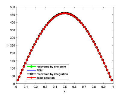
Fig. 1: Left: error of $\|{\bm{u}}-{\bm{w}}_{h}^{c}(p)e^{p}\|$ with respect to $p$ with ${\bm{w}}_{h}^{c}$ computed by (2.8)-(2.9). Right: the recovery from Schrödingerisation by choosing $p>p^{\diamond}=\lambda_{n}(H_{1})T\approx 6$.

6.2 Convergence orders of the discretization for Schrödingerisation

In these tests, we use the numerical simulation to test the convergence rates of the discretization of Schrödingerisation and compare different discretizations for Schrödingerisation.

Firstly, we consider a 1-D case for Maxwell’s equations, For the three-dimensional case, a similar approach can be adopted straightforwardly [25]. The electric field is assumed to have a transverse component $E_{y}$, i.e. ${\bm{E}}=(0,E_{y}(x,t),0)$. The magnetic field is aligned with the z direction and its magnitude is denoted by $B_{z}$, i.e. ${\bm{B}}=(0,0,B_{z}(x,t))$. The reduced Maxwell system is written with periodic boundary condition as,

$$\partial_{t}E_{y}+\partial_{x}B_{z}=-J_{y},\quad\partial_{t}B_{z}+\partial_{x}E_{y}=0,\quad\text{in}\;[0,1].$$ (6.3)

The source term and the initial condition are chosen such that the exact solution is

$$E_{y}=\cos(2\pi x)/(2\pi)-1/(2\pi),\quad B_{z}=t\sin(2\pi x).$$

Yee’s scheme [38] for spatial dicretization gives

$$\frac{\mathrm{d}}{\mathrm{d}t}\begin{bmatrix}{\bm{u}}\\ {\bm{r}}\end{bmatrix}=\begin{bmatrix}A&B\\ \textbf{0}&\textbf{0}\end{bmatrix}\begin{bmatrix}{\bm{u}}\\ {\bm{r}}\end{bmatrix},$$ (6.4)

where ${\bm{u}}=\sum\limits_{i=0}^{n-2}E_{i+1}|i\rangle+\sum\limits_{i=0}^{n-1}B_{i+\frac{1}{2}}|n-1+i\rangle$ and ${\bm{r}}=\sum\limits_{i=0}^{n-2}|i\rangle$. The matrix $A\in\mathbb{R}^{2n-1,2n-1}$ and $B\in\mathbb{R}^{2n-1,n-1}$ are defined by

$$A=\begin{bmatrix}\textbf{0}&-D_{x}\\ D_{x}^{\top}&\textbf{0}\end{bmatrix},\quad B=\begin{bmatrix}-J_{y}\\ \textbf{0}\end{bmatrix},\quad D_{x}=\frac{1}{h}\begin{bmatrix}1&-1&0&\cdots&0\\ &1&-1&\cdots&0\\ &&\ddots&\ddots&\\ &&&1&-1\end{bmatrix}\in\mathbb{R}^{n-1,n},$$ (6.5)

where ${\bm{J}}_{y}=\text{diag}\{{\bm{J}}_{h}\}$ with ${\bm{J}}_{h}=\sum\limits_{i=1}^{n-1}J_{y}(x_{i},t)|i\rangle$. Then $\tilde{H}_{1}$ is obtained by $\tilde{H}_{1}=\begin{bmatrix}\textbf{0}&B/2\\ B/2&\textbf{0}\end{bmatrix}.$ Obviously, one gets $\lambda(\tilde{H}_{1})=\mathscr{O}(|b|/2)=\mathscr{O}(\max_{x,t}\{J_{y}\}/2)$.

$\triangle p$	$\frac{4\pi}{2^{7}}$	order	$\frac{4\pi}{2^{8}}$	order	$\frac{4\pi}{2^{9}}$	order
$\frac{\|{\bm{w}}_{h}^{d}-{\bm{w}}\|_{{\bm{L}}^{2}([2,4\pi])}}{\|{\bm{w}}\|_{{\bm{L}}^{2}([2,4\pi])}}$	1.8693e-04	-	4.1018e-05	2.18	8.8194e-06	2.21
$X$	$10$	order	$20$	order	$40$	order
$\frac{\|{\bm{w}}_{h}^{c}-{\bm{w}}\|_{{\bm{L}}^{2}([2,10])}}{\|{\bm{w}}\|_{{\bm{L}}^{2}([2,10])}}$	3.1213e-02	-	9.4042e-03	1.73	2.0023e-03	2.23

Tab. 1: The convergence rates of $\frac{\|{\bm{w}}_{h}^{d}-{\bm{w}}\|_{{\bm{L}}^{2}([2,4\pi])}}{\|{\bm{w}}\|_{{\bm{L}}^{2}([2,4\pi])}}$ and $\frac{\|{\bm{w}}_{h}^{c}-{\bm{w}}\|_{{\bm{L}}^{2}([2,10])}}{\|{\bm{w}}\|_{{\bm{L}}^{2}([2,10])}}$, respectively, where ${\bm{w}}_{h}^{d}$ is computed by (2.8)-(2.9), and ${\bm{w}}_{h}^{c}$ is computed by (2.12)-(2.13).

In this test, we choose $\varepsilon=1$ and the modified smooth initial values (4.25) to test the convergence rates of the discretization for Schrödingerisation. For (2.8), we fix the $p$-domain within $[-4\pi,4\pi]$. For (2.11), we fix the step size of $\xi$ with $\triangle\xi=\frac{10}{2^{7}}$. Tab. 1 shows that the optimal convergence order $\frac{\|{\bm{w}}_{h}^{d}-{\bm{w}}\|_{{\bm{L}}^{2}([2,4\pi])}}{\|{\bm{w}}\|_{{\bm{L}}^{2}([2,4\pi])}}\sim\triangle p^{2}$, $\frac{\|{\bm{w}}_{h}^{c}-{\bm{w}}\|_{{\bm{L}}^{2}([2,10])}}{\|{\bm{w}}\|_{{\bm{L}}^{2}([2,10])}}\sim X^{-1}$ are obtained, respectively. Fig. 2 shows $\|{\bm{w}}_{h}^{c}e^{p}-{\bm{u}}\|$, $\|{\bm{w}}_{h}^{d}e^{p}-{\bm{u}}\|$ with respect to $p$. It implies that it is better to pick the point $p^{*}>p^{\Diamond}$ near $p^{\Diamond}$ to avoid the error being magnified exponentially for large $p^{*}$ when using one point to recover ${\bm{u}}$. According to the proof in Theorem 4.2, the residual of $\|{\bm{w}}_{h}^{c}-{\bm{w}}\|$ contains $\int e^{i\xi p}d\xi$, leading to the oscillation of $\|{\bm{w}}_{h}^{c}e^{p}-{\bm{u}}\|$ in terms of $p$. Therefore, it would be better to apply integration to recover ${\bm{u}}$ when using continuous Fourier transformation for Schrödingerisation.

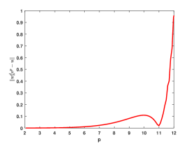
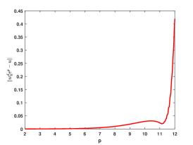
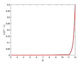
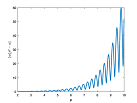
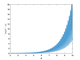
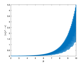
Fig. 2: The first row: the error of discrete Fourier transform defined by $\|{\bm{w}}_{h}^{d}e^{p}-{\bm{u}}\|$ for Schrödingerisation, where ${\bm{w}}_{h}^{d}$ is computed by (2.8) and (2.9), $\triangle p=\frac{4\pi}{2^{7}}$, $\frac{4\pi}{2^{8}}$ and $\frac{4\pi}{2^{9}}$, respectively. The second row: the error of continuous Fourier transform defined by $\|{\bm{w}}_{h}^{c}e^{p}-{\bm{u}}\|$ for Schrödingerisation, where ${\bm{w}}_{h}^{c}$ is computed by (2.12) and (2.13), $X=10$, $20$, $40$, respectively.

Next, we consider the heat equation in domain $[0,1]$ as

$$\partial_{t}u=-\triangle u,\quad u(0)=\sin(\pi x).$$ (6.6)

The Dirichlet boundary conditions $u(0,t)=u(1,t)=0$ are set to obtain the exact solution $u=e^{-\pi^{2}t}\sin(\pi x)$. The spatial discretization is obtained by letting $k=0$ in (6.2). One can check that the eigenvalues of $A$ satisfying $\lambda^{-}_{\max}(H_{1})=\mathscr{O}(\frac{1}{h^{2}})$ and $\lambda(H_{1})\leq 0$ where $H_{1}=(A+A^{\dagger})/2=A$. We use two different Fourier discretizations for Schrödingerisation. The results are shown in Fig. 3 and 4. Since $\lambda_{\max}^{-}(H_{1})$ is too large to make the $p$ domain satisfying (4.27), it is difficult to get an approximate solution with small relative error (see Fig. 3). However, the approximation computed by the continuous Fourier transform agrees well with the exact solution (see Fig. 4). Comparing with Fig. 2 and 3, 4, we make the following summary.

• Compare two Fourier discretization of Schrödingerisation – (2.8) and (2.12). When $\lambda_{\max}^{-}(H_{1})$ is not particularly large, we refer to (2.8) to discretize the Schrödingerized equations. Compared with (2.11), the discrete Fourier transform for Schrödingerisation (2.8) has smaller error and higher-order convergence rates from Tab. 1. However, big $\lambda_{\max}^{-}(H_{1})$ requires a particularly large $p$ domain, which makes it hard to obtain a satisfactory approximation, in this case, it is more recommended to use the continuous Fourier transform for Schrödingerisation.

• Compare two recovery methods–(3.5) and (3.11). According to Fig. 2, recovery of the primitive variables by a point is suitable for discrete Fourier transform (2.8), and recovery of the solution by integration is suitable for continuous Fourier transform (2.11) due to the oscillation of the error with $p$.

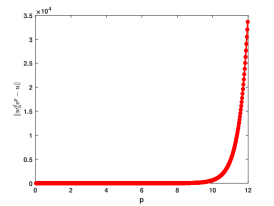
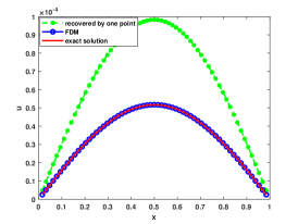
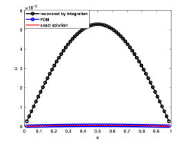
Fig. 3: Left: the error of discrete Fourier transform for Schrödingerisation defined by $\|{\bm{w}}_{h}^{d}e^{p}-{\bm{u}}\|$, where ${\bm{w}}_{h}^{d}$ is computed by (2.8), (2.9) with $\triangle p=\frac{4\pi}{2^{10}}$, $p\in[-4\pi,4\pi]$. Middle: recovery from one point computed by (3.5). Right: recovery from integration computed by (3.11).

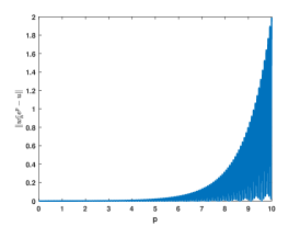
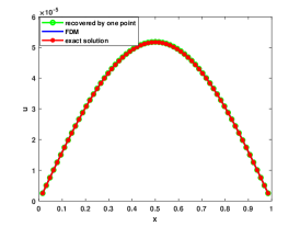
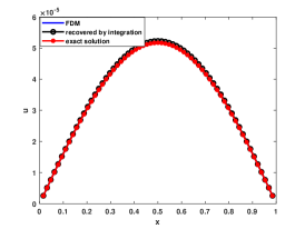
Fig. 4: Left: the error of continuous Fourier transform for Schrödingerisation defined by $\|{\bm{w}}_{h}^{c}e^{p}-{\bm{u}}\|$, where ${\bm{w}}_{h}^{c}$ is computed by (2.12), (2.13) with $X=40$. Middle: recovery from one point computed by (3.5). Right: recovery from integration computed by (3.11).

6.3 An in-homogeneous system with big source terms

In this test, we fix the initial conditions of (6.3) and change the source term by

$$J_{y}=-2000\pi t\cos(2\pi x).$$

It is easy to find $\lambda(\tilde{H}_{1})=\mathscr{O}(10^{3})$. From Fig. 5, we find it is hard to recover ${\bm{u}}$ without using the stretch transformation. By choosing $\varepsilon=10^{-3}$, the recovery from Schrödingerisation agrees well with the exact solution (see Fig. 6). Comparing Tab. 1 and 2, we find that the stretch coefficient dose not affect the relative error and the order of convergence.

$\triangle p$	$\frac{4\pi}{2^{7}}$	order	$\frac{4\pi}{2^{8}}$	order	$\frac{4\pi}{2^{9}}$	order
$\frac{\|{\bm{w}}_{h}^{d}-{\bm{w}}\|_{{\bm{L}}^{2}([2,4\pi])}}{\|{\bm{w}}\|_{{\bm{L}}^{2}([2,4\pi])}}$	1.6872e-04	-	3.6874e-05	2.19	7.5457e-06	2.28
$X$	$10$	order	$20$	order	$40$	order
$\frac{\|{\bm{w}}_{h}^{c}-{\bm{w}}\|_{{\bm{L}}^{2}([2,10])}}{\|{\bm{w}}\|_{{\bm{L}}^{2}([2,10])}}$	2.6798e-02	-	8.1479e-03	1.73	1.7165e-03	2.23

Tab. 2: The convergence rates of $\frac{\|{\bm{w}}_{h}^{d}-{\bm{w}}\|_{{\bm{L}}^{2}([2,4\pi])}}{\|{\bm{w}}\|_{{\bm{L}}^{2}([2,4\pi])}}$ and $\frac{\|{\bm{w}}_{h}^{c}-{\bm{w}}\|_{{\bm{L}}^{2}([2,10])}}{\|{\bm{w}}\|_{{\bm{L}}^{2}([2,10])}}$, respectively, where ${\bm{w}}_{h}^{d}$ is computed by (5.16), (2.9) with $\varepsilon=10^{-3}$, and ${\bm{w}}_{h}^{c}$ is computed by (5.18), (2.13) with $\varepsilon=10^{-3}$.

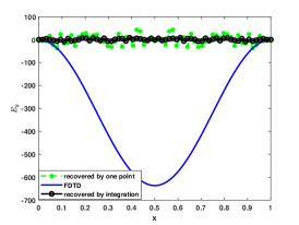
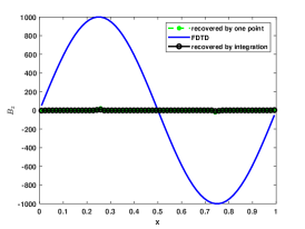
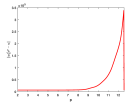
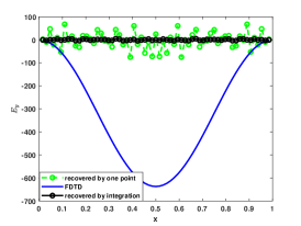
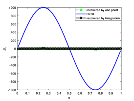
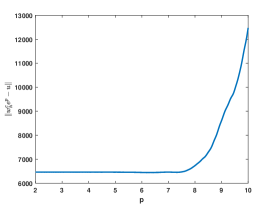
Fig. 5: The first row: results of discrete Fourier transform for Schrödingerisation computed by (5.16) with $\varepsilon=1$, $\triangle p=\frac{4\pi}{2^{9}}$, $p\in[-4\pi,4\pi]$. The second row: results of continuous Fourier transform for Schrödingerisation computed by (5.18) with $\varepsilon=1$, $\triangle\xi=\frac{10}{2^{7}}$, $X=40$.

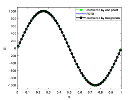
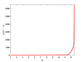
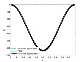
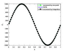
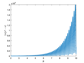
Fig. 6: The first row: results of discrete Fourier transform for Schrödingerisation computed by (5.16) with $\varepsilon=10^{-3}$, $\triangle p=\frac{4\pi}{2^{8}}$, $p\in[-4\pi,4\pi]$. The second row: results of continuous Fourier transform for Schrödingerisation computed by (5.18) with $\varepsilon=10^{-3}$, $\triangle\xi=\frac{10}{2^{7}}$, $X=20$.

7 Conclusions

In this paper, we present some analysis and numerical investigations of the Schrödingerisation of a general linear system with a source term. Conditions under which to recover the original variables are studied theoretically and numerically, for systems that can contain unstable modes. We give the implementation details of the discretization of the Schrödingerisation and prove the corresponding error estimates and convergence orders. In addition, we homogenize the source term by using the stretch transformation and show that the stretch coefficient does not affect the error estimate of the quantum simulation.

As can be seen from the analysis, it is difficult to recover the target variables when the evolution matrix has large positive eigenvalues, as in chaotic systems. Our method provides a simple and general way to construct stable (including both classical and quantum) computational methods for unstable, ill-posed problems. This will be the subject of our further investigation.

References

- [1] B. Şahinoğlu and R. D. Somma. Hamiltonian simulation in the low-energy subspace. npj Quantum Information, 7(119), 2021.
- [2] D. An, D. Fang, and L. Lin. Time-dependent unbounded hamiltonian simulation with vector norm scaling. Quantum, 5(459), 2021.
- [3] D. An, D. Fang, and L. Lin. Time-dependent hamiltonian simulation of highly oscillatory dynamics and superconvergence for schrödinger equation. Quantum, 6(690), 2022.
- [4] D. An, J. Liu, and L. Lin. Linear combination of hamiltonian simulation for non-unitary dynamics with optimal state preparation cost. Phys. Rev. Lett., 131(15):150603, 2023.
- [5] D. W. Berry, G. Ahokas, R. Cleve, and B. C. Sanders. Efficient quantum algorithms for simulating sparse hamiltonians. Commun. Math. Phys., 270:359–371, 2007.
- [6] D. W. Berry and A. M. Childs. Black-box hamiltonian simulation and unitary implementation. Quantum Inf. Comput., 12:39–62, 2012.
- [7] D. W. Berry, A. M. Childs, R. Cleve, R. Kothari, and R. D. Somma. Exponential improvement in precision for simulating sparse hamiltonians. In: Proceedings of the 46th Annual ACM Symposium on Theory of Computing, page 283–292, 2014.
- [8] D. W. Berry, A. M. Childs, R. Cleve, R. Kothari, and R. D. Somma. Simulating hamiltonian dynamics with a truncatd taylor series. Phys. Rev. Lett., 090502, 2015.
- [9] D. W. Berry, A. M. Childs, and R. Kothari. Hamiltonian simulation with nearly optimal dependence on all parameters. IEEE 56th annual symposium on foundations of computer science, 2015.
- [10] D. W. Berry, A. M. Childs, Y. Su, X. Wang, and N. Wiebe. Time-dependent hamiltonian simulation with l1-norm scaling. Quantum, 4(254), 2020.
- [11] D. W. Berry, R. Cleve, and S. Gharibian. Gate-efficient discrete simulations of continuous-time quantum query algorithms. Quantum Inf. Comput., 14:1–30, 2014.
- [12] D. W. Berry and L. Novo. Corrected quantum walk for optimal hamiltonian simulation. Quantum Inf. Comput., 1295:15–16, 2016.
- [13] G. Brassard, P. Hoyer, M. Mosca, and A. Tapp. Quantum amplitude amplification and estimation. Contemp. Math., 305:53–74.
- [14] E. Campbell. Random compiler for fast hamiltonian simulation. Phys. Rev. Lett., 123(7), 2019.
- [15] Y. Cao, S. Jin, and N. Liu. Quantum simulation for time-dependent hamiltonians – with applications to non-autonomous ordinary and partial differential equations. arXiv:2312.02817v1, 2023.
- [16] A. M. Childs, D. Maslov, Y. Nam, N. J. Ross, and Y. Su. Toward the first quantum simulation with quantum speedup. Proc. Nat. Acad. Sci. India Sect. A, 115:9456–9461, 2018.
- [17] D. DiVincenzo. Quantum computation. Science, 270(5234):255–261, 1995.
- [18] A. Ekert, R. Jozsa, and P. Marcer. Quantum algorithms: Entanglement-enhanced information processing. Philos. Trans. Royal Soc. A, 356(1743):1769–1782, 1998.
- [19] L. C. Evans. Partial differential equations. American Mathematical Society, 2016.
- [20] R. A. Horn and C. R. Johnson. Matrix analysis. Cambridge university press, 2012.
- [21] S. Jin, X. Li, N. Liu, and Y. Yu. Quantum simulation for partial differential equations with physical boundary or interface conditions. J. Comput. Phys., 112707, 2024.
- [22] S. Jin and N. Liu. Analog quantum simulation of partial differential equations. arXiv:2308.00646, 2023.
- [23] S. Jin and N. Liu. Quantum simulation of discrete linear dynamical systems and simple iterative methods in linear algebra via schrodingerisation. arXiv:2304.02865, 2023.
- [24] S. Jin, N. Liu, X Li, and Y. Yu. Quantum simulation for quantum dynamics with artificial boundary conditions. arXiv:2304.00667, 2023.
- [25] S. Jin, N. Liu, and C. Ma. Quantum simulation of maxwell’s equations via schrödingersation. arXiv:2308.08408, 2023.
- [26] S. Jin, N. Liu, and Y. Yu. Quantum simulation of partial differential equations via schrodingerisation. arXiv preprint arXiv:2212.13969., 2022.
- [27] S. Jin, N. Liu, and Y. Yu. Quantum simulation of partial differential equations via schrodingerisation: technical details. arXiv preprint arXiv:2212.14703, 2022.
- [28] S. Jin, N. Liu, and Y. Yu. Quantum simulation of partial differential equations: Applications and detailed anlysis. Phys. Rev. A, 108(032603), 2023.
- [29] Shi Jin and Nana Liu. Quantum simulation of discrete linear dynamical systems and simple iterative methods in linear algebra via schrodingerisation. arXiv preprint arXiv:2304.02865, 2023.
- [30] C. S. Lam. Decomposition of time-ordered products and path-ordered exponentials. J. Math. Phys., (10):5543–5558, 1998.
- [31] G. H. Low and I. L. Chuang. Optimal hamiltonian simulation by quantum signal processing. Phys. Rev. Lett., 118:010501, 2017.
- [32] M. A. Nielsen and I. L. Chuang. Quantum Computation and Quantum Information. Cambridge University Press, 2000.
- [33] L. Novo and D. W. Berry. Improved hamiltonian simulation via a truncated taylor series and corrections. Quantum Inf. Comput., 17:0623, 2017.
- [34] D. Poulin, A. Qarry, R. D. Somma, and F. Verstraete. Quantum simulation of time-dependent hamiltonians and the convenient illusion of hilbert space. Phys. Rev. Lett., 106:170501, 2011.
- [35] J. Shen, T. Tang, and L. Wang. Spectral methods. Springer-Verlag Berliln Heidelberg, 2011.
- [36] P. W. Shor. Algorithms for quantum computation: discrete logarithms and factoring. Proceedings 35th annual symposium on foundations of computer science. IEEE, pages 124–134, 1994.
- [37] A. Steane. Quantum computing. Rep. Progr. Phys., 61(2):117–173, 1998.
- [38] A. Taflove, S. C. Hagness, and M. Piket-May. Computational electromagnetics: the finite-difference time-domain method. The Electrical Engineering Handbook, 3:629–670, 2005.