A Quick Introduction to Quantum Machine Learning
for Non-Practitioners
 

Abstract

Quantum computing has quickly become a highly active research area, and quantum machine learning has emerged as a potential manifestation of classical machine learning on quantum hardware. The widespread successes of classical machine learning in classification problems are extremely attractive, however they come at the cost of an exponential growth of parameters in modern network architectures (e.g. GPT). A possible benefit in addressing such problems with quantum networks is an increased expressibility of quantum bits over classical bits, which through quantum machine learning leads to an increased expressibility of a quantum neuron.

Quantum computing is founded on the premise of using particles that are governed by quantum mechanics for the purposes of computation by leveraging key aspects such as superposition and entanglement. These properties have theoretical advantage in representing and manipulating information. Namely superposition allows for a fundamental bit of information to encode a continuous spectrum, while entanglement allows non-local effects to manipulate encoded information. Circuits of quantum gates are used to perform quantum computations, and when parameterized, can be optimized, or trained, using traditional methods in optimization. This leads to a quantum machine learning framework where classical information embedded in quantum bits can take advantage of quantum phenomena and increased expressibility for a potential reduction in network size and training time on quantum hardware.

This manuscript serves as introductory material for researchers that are new to the areas of quantum mechanics and machine learning, in order to decrease the timeframe needed for developing new expertise. The notion of a Turing machine is used as a foundation and motivation for creating computers out of quantum hardware. Next, basic principles and notation of quantum mechanics are introduced, including superposition, phase space on the Bloch sphere, and entanglement of multiple quantum bits. A basic review of classical digital logic is used to propose notions of quantum gates that may leverage these key properties by a universal set of quantum gates. Next, we introduce classical deep learning concepts such as the artificial neural network, the gradient descent algorithm and its stochastic generalization, and the standard backpropagation approach to training a neural network. These are used as a foundation for introducing trainable quantum circuits as neural networks, including a derivation of the analogous gradient descent approach and its generalizations and methods of encoding classical information in a quantum circuit. Finally, these are topics are combined in an illustrative example problem that highlights a potential advantage of quantum neural networks. The accompanying appendices offer greater detail of various derivations that are provided throughout the manuscript.

1 Why Quantum Computing

The notion of a universal computer was first characterized by the description of the Turing machine [1] based on an infinitely long tape, or computation register, which through the machine could be used to encode any algorithm. These notions, along with the advent of the transistor, eventually led to the von Neumann architecture of computing we have today, where a central processing unit (CPU) performs sequential operations on an encoded stream of information, and separately stores this information in a memory register. With the trend of increasing transistor density per unit area, eventually a limit could be perceived. In addition, the polynomial time computational complexity constraint of this computing architecture, as suggested by the Church-Turing thesis, made the quest for alternative architectures inevitable [2].

The idea of leveraging quantum physics to perform computations was first suggested by Feynman, and is by no means the only alternative to the von Neumann architecture (see [3, 4, 5]), however its appeal is based on the ability to leverage attractive properties such as superposition and entanglement, which allow for a unique framework. Herein, one must carefully construct algorithms which yield a choreography of operations that use sequential constructive and destructive interference to promote the correct solution in probability while effectively cancelling out the probability of incorrect solutions, all without a-priori knowledge of the correct solution. In principle, this approach promises an exponential speedup over the von Neumann architecture [6].

The novelty and unique challenges of leveraging quantum physics for computing has led to not just one, but numerous computing architectures explored by a growing contingent of companies and organizations, each seeking to establish their approach as the dominant approach, and to be the first to demonstrate quantum supremacy on a large-scale device. Among these are: a) using superconducting qubits (often referred to as SQUIDs) by IBM, Google, USTC, and Rigetti, b) trapped ions by IonQ and others, c) photonics by Xanadu and others, and trapped Rydberg atoms by QuEra and others. Beyond these hardware implementations, are several other floating notions, such as building quantum computing on qudits (d-level quantum bits, e.g. ternary quantum bit) as opposed to the binary quantum bit (qubit) [7], as well as abandoning the discrete framework altogether and instead building computing on a continuum quantum state [8, 9].

Outside the goal of universal quantum computing are also specific quantum realizations for specific applications, as in the case of quantum annealing [10, 11] for optimization problems, and quantum machine learning [2, 12] for learning problems. The rapid and heavy investment in quantum computing has led to a so-called race for quantum supremacy in which proponents suggest it can be achieved as soon as the early 2030s [13], yet there remain substantial hurdles before this dream may be realized.

2 Quantum Computing Overview

2.1 Quantum Physics - Notation and Introduction

Quantum computing relies on the manipulation and measurement of quantum phenomena in order to process information. The behavior of quantum phenomena is described by quantum physics, so an understanding of quantum computing necessitates a basic understanding of quantum physics. Quantum physics introduces math notation, known as Dirac notation, which is often quite foreign to other disciplines yet simplifies the introduction of main concepts and carries over to quantum computing. Dirac notation utilizes linear algebra, probability and statistics, as well as notational conventions used in physics.

Linear algebra is used in Dirac notation to describe quantum states as vectors, and to describe the physical processes that can impart change to a quantum state as matrices, which in quantum literature are referred to as operators. Operators ‘operate’ on these quantum states to give some new quantum state. A column vector is by convention used to represent some physical quantum state, for example whether an electron is in the spin up state or spin down state or a photon is in the horizontal or vertical linear polarization state. A vector state $\psi$ (the variable $\psi$ is often used in literature to describe a generic quantum state, usually called a ‘wavefunction’) with two quantities would normally be written as:

$$\vec{\psi}=\begin{bmatrix}a\\ b\end{bmatrix}.$$ (1)

In Dirac notation, the vector state $\psi$ would be written as:

$$|\psi\rangle=\begin{bmatrix}a\\ b\end{bmatrix},$$ (2)

where $|\cdot\rangle$ is the right side of a bracket $\langle\cdot|\cdot\rangle$ and is called a “ket” vector. The complex conjugate transpose of a vector state is also widely used, and is written as:

$$\vec{\psi}^{*\mathsf{T}}=[a^{*}\;\;\;b^{*}]=\vec{\psi}^{\dagger},$$ (3)

where $*$ is the complex conjugate, $\cdot^{\mathsf{T}}$ is the transpose, and the dagger $\cdot^{\dagger}$ is shorthand notation in quantum physics for the conjugate transpose. In Dirac notation, the complex conjugate transposed of a vector state $\psi$ is written as:

$$\langle\psi|=[a^{*}\;\;\;b^{*}],$$ (4)

where $\langle\cdot|$ is the left side of the bracket $\langle\cdot|\cdot\rangle$ and is called a “bra” vector. A bra and a ket written next to each other in a full bracket denotes an inner product between the two vector states:

$$\langle\psi_{1}|\psi_{2}\rangle=\vec{\psi_{1}}^{\dagger}\cdot\vec{\psi_{2}}=[a_{1}^{*}\;\;\;b_{1}^{*}]\cdot\begin{bmatrix}a_{2}\\ b_{2}\end{bmatrix}=a_{1}^{*}a_{2}+b_{1}^{*}b_{2}.$$ (5)

Unitary operators, represented by matrices, are used to change the quantum state. For example, some state $\psi_{i}$ can be modified to another state, $\psi_{i+1}$ after the application of an operator $\hat{U}$ (the hat $\hat{\cdot}$ symbol is often used to denote an operator, though it is not always used). Operators are usually given capital letters for variable names, and a unitary operator is a special type of operator that satisfies the property:

$$\hat{U}\hat{U}^{\dagger}=\hat{U}^{\dagger}\hat{U}=\hat{I},$$ (6)

where $\hat{I}$ is the identity operator and corresponds to imparting no change to a quantum state. The action of an operator, represented as a matrix, is written as:

$$|\psi_{i+1}\rangle=\hat{U}|\psi_{i}\rangle=\begin{bmatrix}u_{11}&u_{12}\\ u_{21}&u_{22}\end{bmatrix}\begin{bmatrix}a_{i}\\ b_{i}\end{bmatrix}=\begin{bmatrix}u_{11}a_{i}+u_{12}b_{i}\\ u_{21}a_{i}+u_{22}b_{i}\end{bmatrix}=\begin{bmatrix}a_{i+1}\\ b_{i+1}\end{bmatrix}.$$ (7)

One can similarly apply complex conjugates and transposes to an operator,

$$\hat{U}^{\dagger}=\begin{bmatrix}u_{11}^{*}&u_{21}^{*}\\ u_{12}^{*}&u_{22}^{*}\end{bmatrix},$$ (8)

and the dagger of an operator is typically applied to bra vectors to update them:

$$\langle\psi_{i+1}|=\langle\psi_{i}|\hat{U}^{\dagger}=[a_{i}^{*}\;\;\;b_{i}^{*}]\begin{bmatrix}u_{11}^{*}&u_{21}^{*}\\ u_{12}^{*}&u_{22}^{*}\end{bmatrix}=[a_{i}^{*}u_{11}^{*}+b_{i}^{*}u_{12}^{*}\;\;\;a_{i}^{*}u_{21}^{*}+b_{i}^{*}u_{22}^{*}]=[a_{i+1}^{*}\;\;\;b_{i+1}^{*}].$$ (9)

Some operators are used to represent measurable properties of quantum systems and are called ‘observables’ or ‘observable operators’. These operators satisfy a slightly weaker requirement of being Hermitian. Hermitian operators are defined by satisfying the following relation:

$$\hat{A}=\hat{A}^{\dagger}.$$ (10)

An important property of Hermitian operators is that one can easily show that they have all real eigenvalues despite having potentially all complex entries. Furthermore, Hermitian operators typically represent ‘measurable’ operators, and in such cases their eigenvalues correspond to familiar quantities such as position, momentum, energy, etc., which also must be real-valued.

The average value of all possible outcomes, based on the probability of each outcome, is referred to as the expectation value (or expected value) of that observable with respect to that quantum state. In Dirac notation, the expectation value is expressed as:

$$\langle\psi|\hat{A}|\psi\rangle,$$ (11)

where $\hat{A}$ is some observable (which we represent here by a matrix), and $|\psi\rangle$ is the quantum state just before the state is measured. The expectation value describes the average measurement outcome, so despite the discrete values of single measurements, an expectation value can (and usually will) give a non-discrete value that does not correspond to a single possible measurement outcome. The possible discrete-valued outcomes of each measurement are given by the eigenvalues of observable $\hat{A}$.

Performing the calculation above will yield the average of the possible outcomes weighted by the probability of each outcome occurring. Expectation values can also be estimated empirically by performing repeated measurements and averaging the results. The probability will be inherent in the empirical histogram of each of the possible outcomes, and if measured an infinite number of times would result in the exact expectation value. Since infinite measurements are not practically feasible, an estimate for the expectation value can be obtained by a finite number of measurements and is often treated as the empirical expectation.

Another important calculation in quantum physics is the probability of some general quantum state $|\psi\rangle$ being in the specified, known state $|\phi\rangle$. This is calculated by the magnitude squared of the inner product between $|\psi\rangle$ and $|\phi\rangle$, which in Dirac notation is represented as:

$$|\langle\phi|\psi\rangle|^{2}=(\langle\phi|\psi\rangle)^{\dagger}\langle\phi|\psi\rangle=\langle\psi|\phi\rangle\langle\phi|\psi\rangle$$ (12)

The inner product $\langle\phi|\psi\rangle$ is the projection of the state $|\psi\rangle$ onto the desired measurement state $|\phi\rangle$. The inner product describes the ‘amount of overlap’ due to the projection, and is called the amplitude of the probability or the ‘probability amplitude’. The square of the magnitude of the probability amplitude (which can also be computed by multiplication of the inner product with its complex conjugate), gives a real value that corresponds to the probability of finding the state $|\psi\rangle$ in the state $|\phi\rangle$ when measured.

In quantum computing, most calculations are performed in the computational basis formed by the zero state $|0\rangle$ and the one state $|1\rangle$ where:

$$\begin{array}[]{l c r}|0\rangle=\begin{bmatrix}1\\ 0\end{bmatrix}&\text{and}&|1\rangle=\begin{bmatrix}0\\ 1\end{bmatrix}.\end{array}$$ (13)

These states are unit vectors because they have a norm (or magnitude, computed as the inner product of a state with itself) of one:

$$\begin{array}[]{l c r}\langle 0|0\rangle=1&\text{and}&\langle 1|1\rangle=1.\end{array}$$ (14)

They are also orthogonal to each other, meaning inner products with each other yield zero:

$$\begin{array}[]{l c r}\langle 0|1\rangle=0&\text{and}&\langle 1|0\rangle=0.\end{array}$$ (15)

Finally, the basis is ‘complete’, meaning that any arbitrary vector can be written as a linear combination of these two basis elements:

$$|\psi\rangle=\begin{bmatrix}a\\ b\end{bmatrix}=a\begin{bmatrix}1\\ 0\end{bmatrix}+b\begin{bmatrix}0\\ 1\end{bmatrix}$$ (16)

Together, these three properties describe the basis as being a complete orthonormal basis.

So far these states seem similar to the binary zeros and ones that are used to represent values in classical computing, however quantum mechanics offers more possible states, which quantum computing seeks to utilize. While

$$\begin{array}[]{l c r}|\psi\rangle=\begin{bmatrix}1\\ 0\end{bmatrix}&\text{and}&|\psi\rangle=\begin{bmatrix}0\\ 1\end{bmatrix}\end{array}$$ (17)

would be the only possible states in a classical computing scheme, the state

$$|\psi\rangle=\begin{bmatrix}1\\ 1\end{bmatrix}$$ (18)

is a legitimate, though unnormalized, state in quantum mechanics. Normalization factors need to be added to ensure state probabilities sum to unity, which will be elucidated by an example. First, the importance of this state being allowed should be highlighted. The state $|\psi\rangle=\begin{bmatrix}1\\ 1\end{bmatrix}$ is a linear combination of the zero state and the one state:

$$|\psi\rangle=\begin{bmatrix}1\\ 1\end{bmatrix}=\begin{bmatrix}1\\ 0\end{bmatrix}+\begin{bmatrix}0\\ 1\end{bmatrix}=|0\rangle+|1\rangle,$$ (19)

and represents some quantum state at a certain point or time before measurement. The fact that multiple possible states are present simultaneously is called superposition, and is a property unique to quantum mechanics. This superposition of states is itself a quantum state; operations and gates applied to the state $|\psi\rangle$ are applied in their normal manner and act on both parts of the state present in the superposition state simultaneously. This key quantum phenomenon leads to a larger computational space that quantum computing seeks to leverage; the classical binary representation is replaced with a continuous space of possible superposition states.

However, once a measurement is made only one of the possible measurable values remains, which was predicted with some probability. So before measurement, both quantum states exist simultaneously in the quantum superposition state, but upon measurement this quantum state “collapses”, and only one basis state is observed while the information for the other state is lost. This probability is mathematically determined by the complex coefficients that multiply each basis element, which are also used to normalize the quantum state.

Now to show why those coefficients are needed, a counter example is presented. Starting with the unnormalized superposition state (without coefficients) introduced earlier:

$$|\psi\rangle=|0\rangle+|1\rangle=\begin{bmatrix}1\\ 0\end{bmatrix}+\begin{bmatrix}0\\ 1\end{bmatrix}=\begin{bmatrix}1\\ 1\end{bmatrix}.$$ (20)

If we take its norm

$$\langle\psi|\psi\rangle=[1^{*}\;\;\;1^{*}]\begin{bmatrix}1\\ 1\end{bmatrix}=2,$$ (21)

we obtain a value of 2. The issue with this becomes apparent when the magnitude of the inner product is squared:

$$|\langle\psi|\psi\rangle|^{2}=(\langle\psi|\psi\rangle)^{\dagger}\langle\psi|\psi\rangle=\langle\psi|\psi\rangle\langle\psi|\psi\rangle=2\cdot 2=4$$ (22)

As described earlier, the magnitude of the inner product of two states squared gives the probability that one state will be in the other state when measured. If the same operation is performed on a state with itself, it yields the probability of the state being in its own state, which must yield a probability of 1 or 100%. Without any normalization coefficients, this calculation gives a probability of 4, or 400%, which is a nonsensical and nonphysical result. Therefore, a condition is imposed that the magnitude of the norm of a state squared must always give a probability of one to ensure the physics remains consistent and logical:

$$|\langle\psi|\psi\rangle|^{2}\equiv 1$$ (23)

This condition also implies that

$$|\langle\psi|\psi\rangle|^{2}=(\langle\psi|\psi\rangle)^{\dagger}\langle\psi|\psi\rangle=\langle\psi|\psi\rangle\langle\psi|\psi\rangle=(|\langle\psi|\psi\rangle|^{2}=(\langle\psi|\psi\rangle)^{\dagger}\langle\psi|\psi\rangle=\langle\psi|\psi\rangle\langle\psi|\psi\rangle)^{2}\equiv 1,$$

and

$$\langle\psi|\psi\rangle\equiv 1.$$ (24)

Coefficients are added to a state to ensure this condition remains true. This is often referred to as normalization. For the above superposition state:

$$|\psi\rangle=\begin{bmatrix}a\\ b\end{bmatrix}=a|0\rangle+b|1\rangle=a\begin{bmatrix}1\\ 0\end{bmatrix}+b\begin{bmatrix}0\\ 1\end{bmatrix},$$ (25)

this condition gives constraints on $a$ and $b$:

$$\langle\psi|\psi\rangle=[a^{*}\;\;\;b^{*}]\begin{bmatrix}a\\ b\end{bmatrix}=a^{*}a+b*b=1.$$ (26)

The coefficients $a$ and $b$ are also used to describe the probability of measuring the state associated with that coefficient. For example, say a state $|\psi\rangle$ has coefficients $a=1/\sqrt{3}$ and $b=\sqrt{2/3}$:

$$|\psi\rangle=\frac{1}{\sqrt{3}}|0\rangle+\sqrt{\frac{2}{3}}|1\rangle=\frac{1}{\sqrt{3}}\begin{bmatrix}1\\ 0\end{bmatrix}+\sqrt{\frac{2}{3}}\begin{bmatrix}0\\ 1\end{bmatrix}=\begin{bmatrix}\frac{1}{\sqrt{3}}\\ \sqrt{\frac{2}{3}}\end{bmatrix}.$$ (27)

To calculate the probability of measuring the zero state from this superposition state, take the square of the magnitude of the inner product of this state with the zero state:

$$\begin{split}|\langle 0|\psi\rangle|^{2}&=\left[\frac{1}{\sqrt{3}}\;\;\;\sqrt{\frac{2}{3}}\right]\begin{bmatrix}1\\ 0\end{bmatrix}[1\;\;\;0]\begin{bmatrix}\frac{1}{\sqrt{3}}\\ \sqrt{\frac{2}{3}}\end{bmatrix}\\ &=\left[\frac{1}{\sqrt{3}}\;\;\;\sqrt{\frac{2}{3}}\right]\begin{bmatrix}1&0\\ 0&0\end{bmatrix}\begin{bmatrix}\frac{1}{\sqrt{3}}\\ \sqrt{\frac{2}{3}}\end{bmatrix}=\left[\frac{1}{\sqrt{3}}\;\;\;\sqrt{\frac{2}{3}}\right]\begin{bmatrix}\frac{1}{\sqrt{3}}\\ 0\end{bmatrix}=\frac{1}{3}\end{split}$$ (28)

This means there is a $1/3$ probability of measuring the eigenvalue associated with the “zero” state. Performing a similar calculation for the one state yields $2/3$, meaning there is a $2/3$ probability of measuring the eigenvalue associated with the one state.

It is also important to note that the magnitude squared of $a$ and $b$ gives the respective probabilities of each state’s eigenvalues being measured:

$$\begin{array}[]{l c r}a^{*}a=\frac{1}{3}&\text{and}&b^{*}b=\frac{2}{3}.\end{array}$$ (29)

This can be seen clearly by doing the probability calculations for measuring the zero state and the one state with a generic state $|\psi\rangle=a|0\rangle+b|1\rangle$ where $a$ and $b$ are left as variables.
Zero state:

$$\begin{split}|\langle 0|\psi\rangle|^{2}&=\left[a^{*}\;\;\;b^{*}\right]\begin{bmatrix}1\\ 0\end{bmatrix}[1\;\;\;0]\begin{bmatrix}a\\ b\end{bmatrix}\\ &=\left[a^{*}\;\;\;b^{*}\right]\begin{bmatrix}1&0\\ 0&0\end{bmatrix}\begin{bmatrix}a\\ b\end{bmatrix}=\left[a^{*}\;\;\;b^{*}\right]\begin{bmatrix}a\\ 0\end{bmatrix}=a^{*}a\end{split}$$ (30)

One state:

$$\begin{split}|\langle 1|\psi\rangle|^{2}&=\left[a^{*}\;\;\;b^{*}\right]\begin{bmatrix}0\\ 1\end{bmatrix}[0\;\;\;1]\begin{bmatrix}a\\ b\end{bmatrix}\\ &=\left[a^{*}\;\;\;b^{*}\right]\begin{bmatrix}0&0\\ 0&1\end{bmatrix}\begin{bmatrix}a\\ b\end{bmatrix}=\left[a^{*}\;\;\;b^{*}\right]\begin{bmatrix}0\\ b\end{bmatrix}=b^{*}b\end{split}$$ (31)

For further reading, see references [14, 15, 16, 17, 18].

2.2 Superposition and Entanglement

The two fundamental properties of quantum physics that are leveraged by quantum computing are superposition and entanglement. When operating with qubits, oftentimes the pertinent physical property being leveraged for quantum computing is known as the spin state. Let $|s\rangle$ represent the spin state of a 2-state particle (i.e. spin-up and spin-down). Then superposition is simply an expression of the spin state in terms of its basis elements

$$|s\rangle=\alpha|\text{up}\rangle+\beta|\text{down}\rangle,$$ (32)

where $\alpha,\beta\in\mathbb{C}$ are complex numbers such that the state is normalized, i.e. $|\alpha|^{2}+|\beta|^{2}=1$, $|\text{up}\rangle$ represents the particle being spin-up, and $|\text{down}\rangle$ represents the particle being spin-down. At a given time, the particle is in a linear combination of its two basis states, which is also referred to as being in a superposition of its basis states, as described earlier. Upon measurement, the superposition collapses to a single state outcome, which is often referred to as ‘wave function collapse’.

While this notion is quite simple from the perspective of linear algebra, it is far more interesting from the perspective of probability theory. As explored earlier, these complex coefficients of superposition are closely related to the respective probabilities of each outcome. For this reason, often times they are referred to as probability amplitudes. The association to probabilities in the classical sense comes by squaring these amplitudes, namely

$$\begin{array}[]{cc}P(|\text{up}\rangle)=|\alpha|^{2},&P(|\text{down}\rangle)=|\beta|^{2}.\end{array}$$ (33)

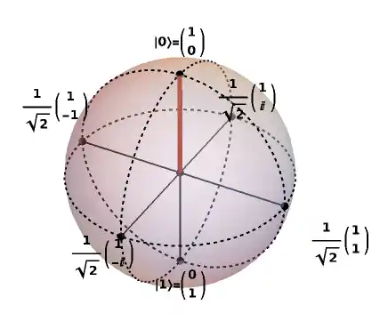
Thus, if for the moment, we take these amplitudes to be purely real, assign the $|\text{up}\rangle$ state to be a 2-vector of unit length pointing in a positive-z direction, and assign the $|\text{down}\rangle$ state to be a 2- vector of unit length pointing in a negative-z direction, then superposition describes a 2D circle of unit length since we require $|\alpha|^{2}+|\beta|^{2}=1$. The vector orthogonal to the z-axis in this circle corresponds to a state $|s\rangle=\frac{1}{\sqrt{2}}|\text{up}\rangle+\frac{1}{\sqrt{2}}|\text{down}\rangle$, where each outcome has equal probability, and this direction is assigned positive-x. Now, returning to the more general case of complex probability amplitudes, the imaginary direction creates a new y axis, and our 2D circular representation becomes a 3D sphere of unit length. This representation is called the Bloch sphere representation, and is depicted in fig. 1.

Figure 1: Bloch sphere representation of a qubit. This figure originated from https://demonstrations.wolfram.com/QubitsOnThePoincareBlochSphere/

The property of entanglement is more complex, but also emerges mathematically in a deceptively simple form. Essentially, if one has two 2-state spin particles

$$\begin{array}[]{l r}|s_{1}\rangle=\frac{1}{\sqrt{2}}|\text{up}\rangle+\frac{1}{\sqrt{2}}|\text{down}\rangle&|s_{2}\rangle=\frac{1}{\sqrt{2}}|\text{down}\rangle+\frac{1}{\sqrt{2}}|\text{up}\rangle\end{array}$$ (34)

and can express their combined state $|s_{1},\,s_{2}\rangle$ as

$$|s_{1},\,s_{2}\rangle=\frac{1}{\sqrt{2}}|\text{up,\, down}\rangle+\frac{1}{\sqrt{2}}|\text{down,\, up}\rangle,$$ (35)

then the two particles are said to be in a state of maximal entanglement. That is, since the total two-particle state is merely expressed by these two two-particle basis states, their states are coupled in such a way that if one were to measure the state of one of the particles (say in the up state), then they would have complete information of the state of the other (which must be in the down state). We say the particles are maximally entangled when each outcome has equal probability (50% for this example). For a two qubit system, there are four such maximally entangled states, known as Bell states. Since the act of measurement of one particle gives complete information of the other, entanglement is a non-local phenomenon, so that virtually all manipulations (i.e. through computing) of the state of one of the particles has some effect on the other particle, regardless of how separated the two particles are.

It is however not the case that all multi-particle systems are entangled. If one can separate the total system state into products of subsystem states, then the state is not entangled. This can be depicted in the following way. Say we have the two-particle system state:

$$|s_{1},\,s_{2}\rangle=\alpha|\text{up,\, down}\rangle+\beta|\text{up,\, up}\rangle,$$ (36)

This system is not in an entangled state because it can be expressed as a product of subsystem states as:

$$|s_{1},\,s_{2}\rangle=|\text{up}\rangle\big{(}\alpha|\text{down}\rangle+\beta|\text{up}\rangle\big{)},$$ (37)

Thus, if we were to measure the first particle, which must be in an up state, we would not gain any information about the state of the second particle, which could still be either in the up or the down state.

2.3 Fundamentals of Classical Computing

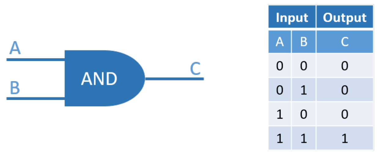
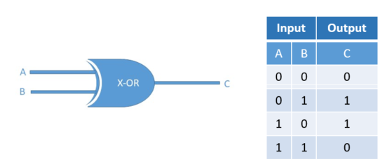
In classical computing, we construct every computation from a fundamental set of building blocks: logical gates. These gates act on pairs of bits by conditionally flipping, summing, or otherwise manipulating the bit pair to yield a single output bit. A simple example is the AND gate shown in fig. 2 The AND gate returns 1 if both A and B are 1, and returns 0 otherwise, which is analogous to multiplying the inputs. The opposite of the AND gate is the NAND (NOT AND) gate, which returns 1 if both A and B are 0, and 0 otherwise. In contrast, the OR gate returns 1 if either A or B is 1, and 0 otherwise, which is analogous to addition. The NOR (NOT OR) gate is its opposite, returning 1 if either A or B is 0, and 1 otherwise. Another important gate is the XOR gate, which returns 1 if A and B are different, and 0 if they are the same, analogous to an equality test. Its opposite, the XNOR gate, returns 0 if A and B are different, and returns 1 if they are the same.

Figure 2: The AND gate

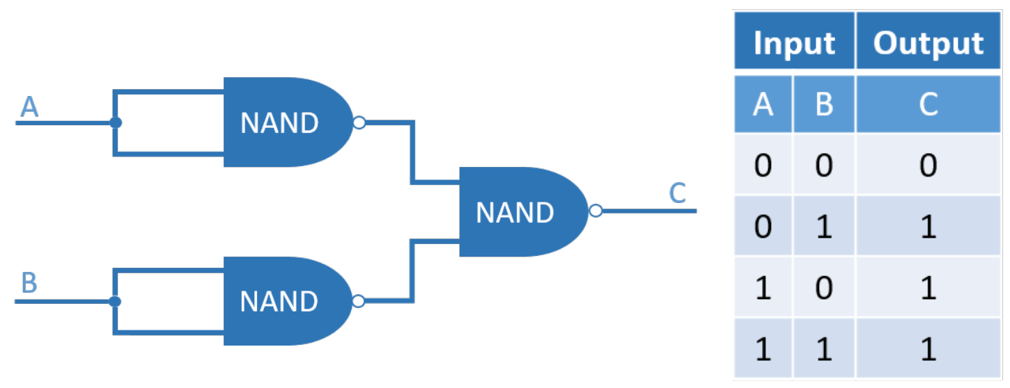
These 6 gates may be applied in a sequence, referred to as a circuit, to create complex networks of logical operations that in turn may be used to construct any algorithm or set of operations. Connecting back to the ideas of Turing, these logical gate building blocks form a universal computer, and are the foundation of modern digital computing. An interesting thing to note is that many of these gates can be created by circuits of a different gate. For example, as depicted in fig. 3, one can construct an OR gate from a circuit of only NAND gates. Actually, one can construct any gate with a circuit of only NAND gates. Similarly, one can construct any gate with a circuit of only NOR gates. We refer to each of these individually as their own universal gate basis set. This is an important notion that will be explored shortly.

Figure 3: The OR gate as a circuit of only NAND gates.

2.4 Fundamentals of Quantum Computing

Similar to the notion of a classical gate, the main thread of quantum computing research seeks to compose quantum computers out of similarly defined logic gates and circuits of logic gates in order to rebuild the classical computing architecture we are familiar with today from the groundup, and thus produce a universal computer out of quantum components. Instead of acting on bits, these components act on quantum bits, or qubits, which are binary representations of quantum states in a 2-state system.

Consider again the spin state of an electron. This state can either be spin-up or spin-down. We previously used the ket notation to describe this as the $|\text{up}\rangle$ state and the $|\text{down}\rangle$ state, but equivalently, one can write them, respectively, as $|0\rangle$ and $|1\rangle$, so that we have encoded the two possible spin state outcomes into a binary representation. These encoded binary representations both simplify our notation, but also generalize to cases where the primary leveraged property is not spin, but some other 2-state property (e.g. the excited/ground state of a Rydberg atom).

The fundamental difference in how this binary state behaves is again the notion of superposition. When each qubit is observed (measured), it must be either in the $|0\rangle$ or the $|1\rangle$ state, however during the sequence of gate operations, it is described by a superposition state

$$|s\rangle=\alpha|0\rangle+\beta|1\rangle.$$ (38)

Thus, similarly, our quantum logic gates must be able to act not only on binary states, but also on any superposition of binary states. Since we always describe states with respect to this basis, it is convenient to write the state vector only in terms of the probability amplitudes $\alpha$ and $\beta$ as

$$|s\rangle=\begin{bmatrix}\alpha\\ \beta\end{bmatrix},$$ (39)

where by convention the top entry corresponds to the amplitude of the $|0\rangle$ basis state and the bottom entry corresponds to the amplitude of the $|1\rangle$ basis state.

Another complication arises from the time-reversibility of quantum mechanics. This requirement states that one must be able to run any sequence of operations either forwards or backwards. Mathematically, this means that every gate operation must be one-to-one, that is, an operation on some unique input produces some unique output. Thus each quantum gate operation must be invertible. This is not true of classical gates; a variety of different inputs can produce the same output, and furthermore, the size of the input space and the size of the output space need not match. This can be clearly seen in the AND logic gate diagram. Two inputs produce a single output, and the output is not unique to the set of inputs (e.g. there are several input pairs that produce 0). Thus, since we have a binary representation, and our input and output sizes must match, it is natural to describe quantum gate operations on single qubits using 2x2 matrices, and quantum gate operations on pairs of qubits using 4x4 matrices.

Finally, operations must preserve the normalization of the quantum state. As was explained earlier, quantum states, and thus gates that operate on quantum states, must preserve probability. Mathematically, this means that for an operator $\hat{A}$ acting on a state $|\psi\rangle$ as $\hat{A}|\psi\rangle=|\psi^{\prime}\rangle$, the new state $|\psi^{\prime}\rangle$ must satisfy $|\psi^{\prime}|^{2}=1$. In the context of operator theory, this requirement implies that gate operations must be unitary and thus satisfy

$$\hat{A}\hat{A}^{\dagger}=\hat{A}\hat{A}^{-1}=\hat{I}.$$ (40)

Since we regard quantum gates as square matrices, we thus require unitary matrices. Notice that this condition is stronger than the invertibility condition, and that any unitary operator is also invertible. As such, typically these two requirements are just expressed as a single unitary requirement, despite originating from different fundamental concepts.

2.5 Single-Qubit Gates

Building on this intuition, we can now attempt to create quantum interpretations of classical logic gates, now represented as unitary matrices. The first gate we will attempt to reproduce is the NOT gate. Assume we have the general single-qubit state as before

$$\begin{array}[]{cc}|s\rangle=\begin{bmatrix}\alpha\\ \beta\end{bmatrix},&|\alpha|^{2}+|\beta|^{2}=1.\end{array}$$ (41)

Now, the NOT gate, often denoted as an operator by $\hat{X}$, should transform a $|0\rangle$ state to a $|1\rangle$ state and vice-versa, so that the amplitudes are flipped

$$\hat{X}\begin{bmatrix}\alpha\\ \beta\end{bmatrix}=\begin{bmatrix}\beta\\ \alpha\end{bmatrix}.$$ (42)

It may be straightforward to see that the only matrix representation of $\hat{X}$ that satisfies this is

$$\hat{X}=\begin{bmatrix}0&1\\ 1&0\end{bmatrix},$$ (43)

which is indeed the quantum NOT gate for a single qubit.

Before we move forward with two-qubit gates, it is interesting to note that while the only nontrivial single classical bit gate is the NOT gate, this is not the case for qubits. There are many non-trivial single-qubit gates, but two important single-qubit gates are the Z gate and the Hadamard gate. The single qubit Z gate is given by

$$\hat{Z}=\begin{bmatrix}1&0\\ 0&-1\end{bmatrix}.$$ (44)

This gate simply flips the sign of the amplitude of the $|1\rangle$ state while leaving the $|0\rangle$ state unchanged. Note that this does not change the probability of the $|1\rangle$ state, since probabilities are squares of amplitudes; instead, it adds a phase of $\pi$.

The Hadamard gate is given by

$$\hat{H}=\frac{1}{\sqrt{2}}\begin{bmatrix}1&1\\ 1&-1\end{bmatrix}.$$ (45)

To understand the effect of this gate, consider the effect of applying $\hat{H}$ to the $|0\rangle$ state:

$$\begin{array}[]{cc}|s\rangle=\begin{bmatrix}1\\ 0\end{bmatrix},&\hat{H}|s\rangle=\frac{1}{\sqrt{2}}\begin{bmatrix}1\\ 1\end{bmatrix}=\frac{1}{\sqrt{2}}\big{(}|0\rangle+|1\rangle\big{)}.\end{array}$$ (46)

Similarly, consider the effect of applying $\hat{H}$ to the $|1\rangle$ state:

$$\begin{array}[]{cc}|s\rangle=\begin{bmatrix}0\\ 1\end{bmatrix},&\hat{H}|s\rangle=\frac{1}{\sqrt{2}}\begin{bmatrix}1\\ -1\end{bmatrix}=\frac{1}{\sqrt{2}}\big{(}|0\rangle-|1\rangle\big{)}.\end{array}$$ (47)

These states are ‘halfway’ between the two basis states, thus the Hadamard gate generates superpositions where each basis state has a probability of 1/2. We may think of these two states as a uniform (symmetric and antisymmetric, resp.) superpositions, since the probabilities are uniformly distributed over outcomes (i.e. basis states). Note that $\hat{H}^{2}=\hat{I}$, so applying the Hadamard gate to a uniform symmetric superposition returns the $|0\rangle$ state, and applying the Hadamard gate to a uniform antisymmetric superposition returns the $|1\rangle$ state. The Hadamard gate is typically used in circuits at the very beginning to generate a uniform superposition state that will be leveraged by the rest of the circuit.

We briefly mention a few other single qubit gates. The $\hat{X}$ and $\hat{Z}$ gates described above are often described as Pauli gates, of which there are three. The Pauli $\hat{Y}$ gate is given by

$$\hat{Y}=\begin{bmatrix}0&-i\\ i&0\end{bmatrix}.$$ (48)

A well-known feature of Pauli operators is that the set $\{\hat{I},\hat{X},\hat{Y},\hat{Z}\}$ forms a basis over the space of 2x2 complex Hermitian operators.

The phase gate $S$ is given by

$$\hat{S}=\begin{bmatrix}1&0\\ 0&i\end{bmatrix},$$ (49)

and is given this name simply because it maps a generic state $|s\rangle=\begin{bmatrix}\alpha\\ \beta\end{bmatrix}$ to the state $|s\rangle=\begin{bmatrix}\alpha\\ i\beta\end{bmatrix}$, thus creating a complex phase.

The $\pi/8$ gate is given the symbol $\hat{T}$ and is given by

$$\hat{T}=\begin{bmatrix}1&0\\ 0&e^{i\pi/4]}\end{bmatrix}.$$ (50)

Note that $\sqrt{i}=e^{i\pi/4}=\cos(\pi/4)+i\sin(\pi/4)=\frac{\sqrt{2}}{2}+i\frac{\sqrt{2}}{2}$, so the $\hat{T}$ gate is the square root of the $\hat{S}$ gate and corresponds to a $\pi/4$ rotation in the complex plane as opposed to a $\pi/2$ rotation with the $\hat{S}$ gate.

Finally, the rotation gates $\hat{R}_{X}(\theta),\hat{R}_{Y}(\theta),\hat{R}_{Z}(\theta)$ are given by

$$\hat{R}_{X}(\theta) =e^{-i\theta/2\cdot\hat{X}}=\begin{bmatrix}\cos\theta/2&-i\sin\theta/2\\ -i\sin\theta/2&\cos\theta/2\end{bmatrix},$$ (51)

$$\hat{R}_{Y}(\theta) =e^{-i\theta/2\cdot\hat{Y}}=\begin{bmatrix}\cos\theta/2&-\sin\theta/2\\ \sin\theta/2&\cos\theta/2\end{bmatrix},$$ (52)

$$\hat{R}_{Z}(\theta) =e^{-i\theta/2\cdot\hat{Z}}=\begin{bmatrix}e^{-i\theta/2}&0\\ 0&e^{i\theta/2}\end{bmatrix}.$$ (53)

These gates are analogous to the rotation matrices in three Cartesian axes, and equivalently rotate the amplitude vector on the Bloch sphere described in fig. 1 about the corresponding axis. In this context of rotations on the Bloch sphere, one can generalize all single-qubit gates to a product of rotations. Namely, any arbitrary single-qubit gate $\hat{U}$ can be decomposed as

$$\hat{U} =e^{i\alpha}\hat{R}_{Z}(\beta)\hat{R}_{Y}(\gamma)\hat{R}_{Z}(\delta)$$ (54)

$$=e^{i\alpha}\begin{bmatrix}e^{-i\beta/2}&0\\ 0&e^{i\beta/2}\end{bmatrix}\begin{bmatrix}\cos\gamma/2&-\sin\gamma/2\\ \sin\gamma/2&\cos\gamma/2\end{bmatrix}\begin{bmatrix}e^{-i\delta/2}&0\\ 0&e^{i\delta/2}\end{bmatrix}$$ (55)

$$=\begin{bmatrix}\cos\gamma/2e^{i(\alpha-\beta/2-\delta/2}&-\sin\gamma/2e^{i(\alpha-\beta/2+\delta/2}\\ \sin\gamma/2e^{i(\alpha+\beta/2-\delta/2}&\cos\gamma/2e^{i(\alpha+\beta/2+\delta/2}\end{bmatrix},$$ (56)

which equates to four parameters on three sequential one-parameter gates (and a phase scaling parameter). This property is quite useful, and may be leveraged for the design of quantum circuits.

2.6 Two-Qubit Gates

In the case of two-qubits we have four outcomes, as opposed to the two in the single-qubit case. These are given by $|00\rangle$, $|01\rangle$, $|10\rangle$, and $|11\rangle$. Thus these states define the computational basis, and one can describe superpositions of these basis states in the general form

$$|s\rangle=\alpha_{00}|00\rangle+\alpha_{01}|01\rangle+\alpha_{10}|10\rangle+\alpha_{11}|11\rangle=\begin{bmatrix}\alpha_{00}\\ \alpha_{01}\\ \alpha_{10}\\ \alpha_{11}\\ \end{bmatrix}$$ (57)

Instead of measuring the entire state as in the case of a single qubit, here we may measure just one of the two qubits, which has a ‘back action’ effect on the other. Say we measure the first qubit. The probability of a $|0\rangle$ state on the first qubit is $|\alpha_{00}|^{2}+|\alpha_{01}|^{2}$, and such an outcome would cause a post-measurement state of

$$|s^{\prime}\rangle=\frac{\alpha_{00}|00\rangle+\alpha_{01}|01\rangle}{\sqrt{|\alpha_{00}|^{2}+|\alpha_{01}|^{2}}}=\frac{1}{\sqrt{|\alpha_{00}|^{2}+|\alpha_{01}|^{2}}}\begin{bmatrix}\alpha_{00}\\ \alpha_{01}\\ 0\\ 0\\ \end{bmatrix}$$ (58)

Two-qubit gates are defined by 4x4 unitary matrices. Among the most famous two-qubit gates is the CNOT gate, given by

$$\text{CNOT}=\begin{bmatrix}1&0&0&0\\ 0&1&0&0\\ 0&0&0&1\\ 0&0&1&0\\ \end{bmatrix}=\begin{bmatrix}\hat{I}&\hat{0}\\ \hat{0}&\hat{X}\end{bmatrix},$$ (59)

where $\hat{0}$ is just the zero matrix. In essence, this gate flips the second qubit if the first qubit contains the $|1\rangle$ state, and does nothing otherwise. To see this, let us apply it to the $|00\rangle$ state:

$$\text{CNOT}|00\rangle=\text{CNOT}\begin{bmatrix}1\\ 0\\ 0\\ 0\\ \end{bmatrix}=\begin{bmatrix}1\\ 0\\ 0\\ 0\\ \end{bmatrix}$$ (60)

Thus when the first qubit is $|0\rangle$, the total state is unchanged. The same occurs to the state $|01\rangle$. Next apply CNOT to the $|10\rangle$ state:

$$\text{CNOT}|10\rangle=\text{CNOT}\begin{bmatrix}0\\ 0\\ 1\\ 0\\ \end{bmatrix}=\begin{bmatrix}0\\ 0\\ 0\\ 1\\ \end{bmatrix}=|11\rangle.$$ (61)

So, the second qubit is flipped when the first qubit contains the $|1\rangle$ state. The same qubit flip occurs in the case of the $|11\rangle$ state, producing $|10\rangle$. More generally,

$$\text{CNOT}\begin{bmatrix}\alpha\\ \beta\\ \gamma\\ \delta\\ \end{bmatrix}=\begin{bmatrix}\alpha\\ \beta\\ \delta\\ \gamma\\ \end{bmatrix},\quad\forall\;\;\alpha,\beta,\gamma,\delta\in\mathbb{C}\;\;\;\text{s.t.}\;\;|\alpha|^{2}+|\beta|^{2}+|\gamma|^{2}+|\delta|^{2}=1.$$ (62)

There are a variety of other two-qubit gates that use the first qubit as a control, and conditionally apply any of the single-qubit gates described above. Examples include the controlled-Z gate (sometimes called CZ), given by

$$\text{controlled-Z}=\begin{bmatrix}1&0&0&0\\ 0&1&0&0\\ 0&0&1&0\\ 0&0&0&-1\\ \end{bmatrix},$$ (63)

and the controlled-phase gate (sometimes called CS), given by

$$\text{controlled-phase}=\begin{bmatrix}1&0&0&0\\ 0&1&0&0\\ 0&0&1&0\\ 0&0&0&i\\ \end{bmatrix}.$$ (64)

Another widely used two-qubit gate is the swap gate, given by

$$\text{swap}=\begin{bmatrix}1&0&0&0\\ 0&0&1&0\\ 0&1&0&0\\ 0&0&0&1\\ \end{bmatrix}.$$ (65)

This gate swaps the $|01\rangle$ state for the $|10\rangle$ state, but leaves other states unaffected. For the generic two-qubit state, we have

$$\text{swap}\begin{bmatrix}\alpha\\ \beta\\ \gamma\\ \delta\\ \end{bmatrix}=\begin{bmatrix}\alpha\\ \gamma\\ \beta\\ \delta\\ \end{bmatrix},\quad\forall\;\;\alpha,\beta,\gamma,\delta\in\mathbb{C}\;\;\;\text{s.t.}\;\;|\alpha|^{2}+|\beta|^{2}+|\gamma|^{2}+|\delta|^{2}=1.$$ (66)

2.7 The Quantum Universal Gate Set

One can quickly see that the richness of the quantum description yields many more usable operations in comparison to the classical case; one has a variety of non-trivial single-qubit gates in contrast to only one non-trivial single bit gate. The basic intuition behind this feature is that quantum gates can cause complex amplitudes to interfere with each other, thus canceling out quantum amplitudes. The feature of having a much larger (uncountably infinite) gate set is much more pronounced with larger multi-qubit operators. The trade-off is that there is significant added complexity to define the universal gate basis set, that is, the set of quantum gates that can produce any unitary operator with sufficient precision.

The challenge with a universal quantum gate set is that it asks to compose a finite set of operators that when put in sequence can produce an uncountably infinite set of n-qubit operators. Thus, the claim of classical universality is weakened for the quantum case by only requiring that we produce any unitary operator with sufficient precision. Some requirements for a universal quantum gate set are that it must be able to create superposition (e.g. Hadamard), that it must be able to create entanglement, and that it must be able to create complex amplitudes as well as real ones.

It has been shown [6] that one such universal quantum gate set is the set $\{\text{CNOT},\hat{S},\hat{R}_{X}(\pi/4)\}$. This set is not unique; one can substitute the $\hat{R}_{X}(\pi/4)$ gate for nearly any rotation gate. Such a universal set enables the quantum computing paradigm to recreate, and generalize the classical computing paradigm.

2.8 Fundamental Challenges of Quantum Computing

Here we describe one of the major difficulties in realizing quantum computers. The increased richness in the expressibility of a quantum superposition state also leads to one of the hardest problems in realizing quantum computing hardware, the problem of quantum error correction [17]. To elucidate this, consider first the classical computing case.

There is always noise that can induce errors in any information processing channel. As a result, even in classical computing there can sometimes be random errors that change a bit from a 0 to a 1, which are called bit flip errors. In classical computing, any channel of communicating information typically appends redundant information to a binary string in order that one can use the redundant information to decode the binary string and recover the intended information despite the error. For example a repetition code with majority voting is a simple classical error correction scheme, where if you intend to communicate a 0 bit, you instead send 000, and similarly to send the 1 bit you send 111. At the receiving end, you simply decode the bit of information based on the majority of 0 or 1 bits communicated, such that you can always protect against a single bit flip error.

In the quantum error correction case, since our qubit states are superpositions of basis states, errors can be understood as changing the probability amplitudes of outcomes. Consider a single qubit as before:

$$\begin{array}[]{cc}|s\rangle=\alpha|0\rangle+\beta|1\rangle=\begin{bmatrix}\alpha\\ \beta\end{bmatrix},&|\alpha|^{2}+|\beta|^{2}=1.\end{array}$$ (67)

As in the case of the $\hat{X}$ gate, the qubit flip yields:

$$|s^{\prime}\rangle=\begin{bmatrix}\beta\\ \alpha\end{bmatrix}=\beta|0\rangle+\alpha|1\rangle.$$ (68)

We can similarly apply the classical repetition code for qubits as:

$$|0\rangle \rightarrow|0\rangle_{L}\equiv|000\rangle, |1\rangle \rightarrow|1\rangle_{L}\equiv|111\rangle$$ (69)

where $|\cdot\rangle_{L}$ corresponds to a logical qubit, so that the single qubit state becomes a three-qubit state:

$$|s\rangle=\alpha|0\rangle_{L}+\beta|1\rangle_{L}.$$ (70)

As before, we can diagnose and correct a single qubit flip by majority voting.

When viewed as a Pauli rotation on the Bloch sphere, a single bit flip is equivalent to a $\pi$ rotation about the x-axis. A fundamental challenge arises upon realizing that the error may rotate our qubit not only about the x-axis, but about any axis in 3D. Thus for a single qubit, we must also perform a similar error diagnosis on the phase flip of a qubit, which has a similar flavor to the bit flip diagnosis, but in a rotated basis corresponding to the x-axis on the Bloch sphere

$$|+\rangle =\frac{1}{\sqrt{2}}\big{(}|0\rangle+|1\rangle)$$ (71)

$$|-\rangle =\frac{1}{\sqrt{2}}\big{(}|0\rangle-|1\rangle)$$ (72)

Logical qubits can be formed in this basis such that a phase flip is diagnosed using a similar majority voting repetition code

A famous result in quantum error correction is known as the Shor code, which can correct an arbitrary error (i.e. any single qubit rotation error), by encoding a 9-qubit logical qubit, however there are codes that can correct any single qubit error by encoding as small as a 5-qubit logical qubit. Thus a quantum computer with only single qubit errors must implement 5 times the number of qubits to attain a given number of logical qubits.

Coupled to this issue is that circuits of increasing numbers of qubits suffer from cross-talk errors, which is when qubits in different channels become undesirably entangled to each other, which requires another level of quantum error correction. There are a variety of quantum errors that appear in hardware that must be diagnosed and corrected, which leads to a complex problem of quantum error correction over arbitrary width quantum circuits. A major challenge in quantum computing is finding codes that reduce the necessary number of qubits to achieve a logical qubit, and building a large enough quantum computer with enough fault tolerance to be able to perform useful operations on these logical qubits.

3 Introduction to Classical Deep Learning Algorithms

The primary goal of machine learning and more specifically deep learning is to optimally approximate some functional mapping that encodes a challenging task. These tasks historically drew heavy inspiration from the everyday tasks that are accomplished by the animal brain. Today, a vast variety of interesting problems are addressed using machine learning and deep learning, from understanding protein folding for better drug discovery [19], to predicting complex weather patterns [20], to processing and/or translating language [21], to autonomous driving [22], to realizing nuclear fusion technology for green energy production [23].

For example when a fox sees the movement of an animal in the distance, its visual cortex must quickly determine if that animal is a bear and the fox should scurry away, or if the animal is a rabbit and the fox should pursue it. This general perception task is highly studied in machine learning literature and known as the task of classification. Here, the natural processes of the brain that classify the visual image of an animal as a bear or a rabbit can be understood as a functional mapping between images and classes of animals.

Another example is based on the motor cortex, where a human might want to pick up a glass of water in order to drink from it. The motor cortex evaluates the current position, velocity, and acceleration of the arm, and the current position of the cup, and must determine the electrical signals that are sent to the arm to cause it to extend and grasp the cup. This general task is also highly studied in robotics literature and known as the task of control (i.e. controlling the hand and arm to grasp the cup). Here again, the natural processes of the brain can be understood as a functional mapping between generalized locations and muscular actuation signals.

This sort of input-output mapping representation of a process or relationship is extremely flexible and general, perhaps universal. Using this framework, the goal of machine learning is to closely approximate the inherent relationship between input and output by a function that contains many, often millions, of flexible parameters often referred to as weights. The mapping is most commonly represented, or modeled, using a highly parameterized Artificial Neural Network (ANN), and the learning in machine learning refers to optimizing the parameters of the model so that it can mimic the process or relationship to high accuracy and precision. The adaptability and expressibility of ANNs have been one of the biggest motivators of their wide spread use. In this section, the basics of ANNs will be covered.

3.1 Overview of Classical Machine Learning Problems and Terminology

In machine learning the general goal is to learn a model from a system with known inputs, and sometimes outputs, so that the model can predict or enhance understanding of the underlying data. In the most general case there are two types of machine learning algorithms; supervised and unsupervised. In the unsupervised case, only the inputs to a system are known and the goal is generally to better describe the data itself. For example, a common unsupervised learning task is called clustering, wherein the machine learning model is attempting to find patterns in the data that identify common characteristics of portions of the data so that homogeneous data is grouped, or clustered, together. In the supervised case, both the inputs and outputs of the system are known and the goal is to accurately predict the systems outputs given the inputs. We will focus on the supervised case as that is more related to our current work.

In the supervised machine learning framework there are again two tasks that machine learning performs; classification and regression. In the classification task machine learning models seek to identify membership of the input data to categories known as classes. For example, determining if an image contains a cat or a dog is understood as determining if the object in the image belongs to the ‘cat’ class or the ‘dog’ class. This type of model will often be referred to as a classifier, as its purpose is generally to assign the correct class to an input, where the outputs are effectively binary ‘yes or ‘no’ for class membership of each class. The regression task is very similar except that instead of being binary in the output, models generally output a continuous value, e.g. given an image of a dog, predict the weight in kilograms of said dog. The differences in these tasks usually comes down to the type of data available and the setup of the optimization problem.

Once the task and model have been defined, the model’s parameters are optimized such that the model fits the data as closely as possible. This optimization procedure is often referred to as training, and is the critical phase of a machine learning algorithm. Here, some function ${\cal F}$ that quantifies some abstract measure of distance, or error, between the predicted labels $\hat{y}$ and the true labels $y$ of the training data $x$ is minimized as

$$\theta_{\text{best}}=\operatornamewithlimits{argmin}_{\theta}{\cal F}\big{(}\hat{y}(\theta,x),y\big{)},$$ (74)

where ${\cal F}\big{(}\hat{y}(\theta,x),y\big{)}$ is the e function to be minimized (e.g. mean squared error) measuring some notion of ‘badness’ of the model’s prediction of the class label. This function is sometimes called an objective function, a cost function, or a loss function depending on the community. All machine learning models can be represented by an equation that maps the input to the desired output, and in this case the predicted labels $\hat{y}$ are a function of the model parameters $\theta$ and the training data $x$.

Before beginning to train, the available data is usually divided into three categories: training data, validation data, and test data. The training data is the data that is used to optimize the model parameters, while the validation data is used to prevent overfitting. Overfitting occurs when the optimization process learns the training data too well and does not generalize to other data. During training, the validation data is evaluated using the same function as the training data, generally referred to as the validation loss, however the model is never updated using the validation loss. The validation loss is monitored over training iterations, and overfitting is generally indicated by an increase in the validation loss for a decreasing training loss. When the validation loss begins increasing, training can be stopped to prevent overfitting. The final step in the machine learning process is the testing phase. Here the model is evaluated to determine true performance. This phase requires a completely blind set of data called test data, i.e. neither the validation nor training data can be used. This ensures that the performance of the model on the test data captures what typical performance would look like in practice.

If we consider a general classification task such as the one described above, the goal of training is to separate the input space into multiple regions where each region contains only a single class label. This clearly requires that the data is separable in some way; and the simplest case is where the data is linearly separable. Let’s assume that our data has two classes, if a straight line can be drawn between the classes that data is linearly separable and any machine learning model will be able to correctly classify this data. This very rarely happens in real world data, thus many advanced models have been developed to handle data of various complexities, such as data that is not linearly separable. One such model will be covered next.

3.2 Neural Networks

The beginnings of ANNs trace back to 1957 with Rosenblatt’s perceptron [24]. The perceptron classifier is a simple linear classifier/regression model. In the perceptron a group of weights are used to transform the input variables into the desired output. The perceptron uses the equation, ${\bf y}={\bf W}{\bf x}$, where ${\bf x}$ is the input vector, ${\bf W}$ are the weights, and ${\bf y}$ is the output which is either a scalar value or a new vector. This is a linear mapping which is severely limited in its real world application as demonstrated by the following example.

The XOR problem is often used for illustrations on the decision boundaries obtained with neural networks. The XOR problem generally consists of four clusters of data which are grouped into two classes. The clusters are generally created in a square, i.e. the four cluster centers are located at (-1, -1), (-1, 1), (1, 1), and (1, -1), with the diagonal clusters labeled as one class and the off-diagonal clusters as the opposite class. The perceptron is shown graphically on the left side of fig. 4, and the image on the right shows the limitations of the perceptron in solving the XOR problem. In the image, the different colors each indicate a different class. Since the perceptron is a linear classifier it can only define a simple linear decision boundary. Therefore, the perceptron is unable to correctly separate the diagonal and off-diagonal classes.

Figure 4: Perceptron Example

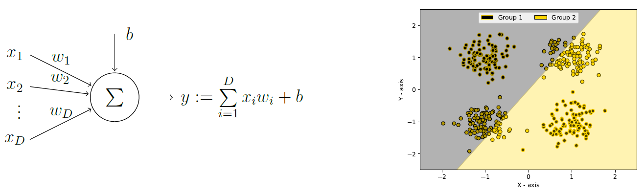
To improve upon the perceptron it was found that performance could be greatly improved by combining multiple perceptrons together. The combination process involves creating layers of perceptrons. A layer is generated by having several perceptrons in parallel, with each perceptron using the same inputs. When combined in this fashion each perceptron is generally called a neuron. As the single perceptron case is simply an inner product between the inputs and the weights, a layer can be seen as a linear mapping from the input space to the space defined by the weights of each neuron. Thus each layer is computed as a matrix multiplication. The output from each linear mapping is then fed into a non-linear function often referred to as an activation function, which is named after its approximation of the step activation of a biological neuron. This process is often referred to as the Wiener method [25], which has the non-linear activation following the summation in fig. 4. The purpose of the non-linear activation is to increase expressibility of the network, as without non-linearities a series of linear mappings will always reduce to a single linear mapping. Stacking multiple layers together, by connecting the outputs of a layer to the inputs of the following layer, creates what is called the Multi-Layered Perceptron (MLP) [26], and is shown in the left side of fig. 5. In the diagram each circle is considered a neuron. The outputs from the final layer, generally called the logits, are often converted to probabilities via the softmax function, which is defined as

$$\sigma({\bf z})_{i}=\frac{e^{\beta z_{i}}}{\sum_{j=1}^{K}e^{\beta z_{j}}},\;\;\;i=1,\dots,K,$$ (75)

where $K$ is e number of logits in the output layer, ${\bf z}$ is the vector of output logits with $z_{i}$ being the $i^{th}$ element of the vector, and $\beta$ is referred to as the temperature which is a hyperparameter that controls the smoothness of the softmax function.

Figure 5: Multilayer Perceptron Example

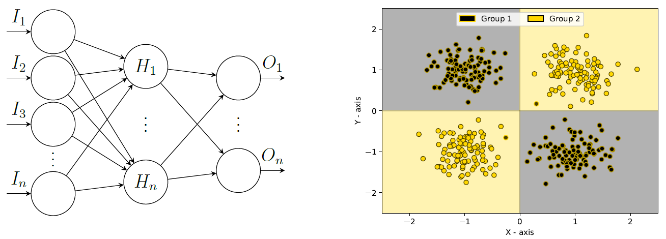
With the addition of multiple layers and non-linearities, the MLP is now capable of classifying data that is not linearly separated, as in the right side of fig. 5. The stacking of layers allows the MLP to define multiple regions that can be separated linearly by the final classification layer. For example, in the XOR problem shown in the right side of fig. 5 the hidden layer can divide the feature space into the four quadrants shown. The classification layer then classifies the quadrants into their proper classes as the first layer projects the data into a space where the quadrants are linearly separable. To be considered a MLP there must be at least three layers: the input layer, the output layer, then at least one hidden layer. The hidden layer(s) fall between the other two layers as shown in the left side of fig. 5. In general multi-layer networks, there are many layers of matrix-vector multiplications which can be expressed as

$$f({\bf x}_{n};{\bf W})=\sigma_{N_{h}}\Bigg{(}{\bf W}_{N_{h}}\sigma_{N_{h-1}}\bigg{(}{\bf W}_{N_{h-1}}\sigma_{N_{h-2}}\Big{(}\cdots\sigma_{1}({\bf W}_{q}{\bf x}_{n})\Big{)}\bigg{)}\Bigg{)},$$ (76)

where ${\bf x}_{n}$ is an input, $N_{h}$ is the number of hidden layers, $\sigma_{h}(\cdot)$, $h=1,2,\dots,N_{h}$ are activation functions, and ${\bf W}$ are the weights. To describe the potential capabilities of the MLP the Universal Approximation Theorem was proved in [27] which states that MLPs are capable of approximating any continuous function to an arbitrary accuracy given that the hidden layer is of sufficient size.

3.3 Shared Weight Neural Networks

The standard MLP is effective for a broad category of tasks, however the MLP also introduces a bias toward interconnectivity of every data point. While this is often a good strategy, it can introduce significant redundancy, and specifically many classification problems rely on images, for which local relationships are more important. In adding more capability to the MLP, the next big advancement was the shared weight network from [28]. This is easiest to visualize via the convolutional neural network (CNN) [29]. Convolution networks are based on the standard convolution operation defined as:

$$(f\ast g_{\theta})[n]=\sum_{m=0}^{N-1}f[m]g_{\theta}[n-m],$$ (77)

where $f$ and $g_{\theta}$ are functions to be convolved, and $g_{\theta}$ is parameterized by $\theta$ and is often referred to as the convolution filter. Note that convolution is usually implemented as correlation in convolution networks, because correlation requires fewer operations and the convolution filter is learned therefore the two are effectively equivalent. To better explain what is happening see fig. 6. In the figure a simple convolution example is shown using two vectors, one of size 4 and another of size 3.

Figure 6: Simple convolution example

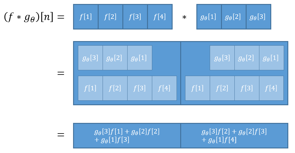
For this demo only the valid portion of the convolution is used meaning only the locations where two vectors fully overlap are used, these two positions are shown in the center line of the figure. The last line of the diagram shows the output of the convolution as an equation of the individual elements of $f$ and $g_{\theta}$. The last line can also be represented as a matrix multiplication as in:

$$(f\ast g_{\theta})[n]=\begin{bmatrix}g_{\theta}[3]&g_{\theta}[2]&g_{\theta}[1]&0\\ 0&g_{\theta}[3]&g_{\theta}[2]&g_{\theta}[1]\end{bmatrix}\begin{bmatrix}f[1]\\ f[2]\\ f[3]\\ f[4]\\ \end{bmatrix}.$$ (78)

With this representation if we write the 2 × 4 matrix as ${\bf W}$ with $w_{n}=g_{\theta}[n]$, and the vector of $f[n]$ as ${\bf x}$, with ${\bf x}_{n}=f[n]$, we are left with exactly the equation of a perceptron, ${\bf y}={\bf W}{\bf x}$ as was seen before. With this new representation we can rewrite the convolution operation we started with as the simple single layer neural network shown in fig. 7.

Figure 7: Simple convolution layer example

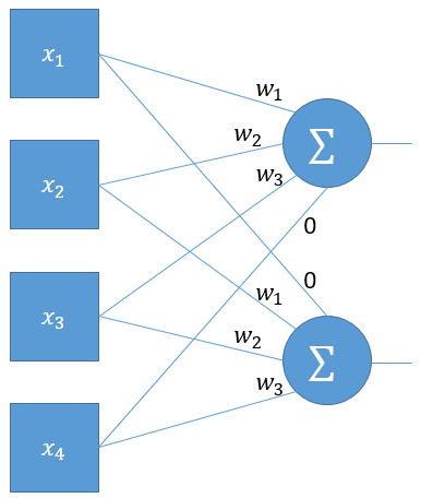
In this representation the weights $\{w_{1},w_{2},w_{3}\}$ are shared across both of the neurons represented by the summation symbols, thus a small set of weights can be shared across the input space. This type of network is in general applied to images, and can dramatically reduce the number of network parameters, which can reduce overfitting, reduce training time, and reduce model complexity.

3.4 Gradient Descent

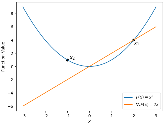
Training for all types of neural networks uses some flavor of gradient descent. Gradient descent is an optimization strategy that is widely used for fitting many different types of models and data. Assuming a convex function, for a given point the sign of the gradient points away from the minimum. For example, in fig. 8, assume we are trying to find the minimum of the function $F(x)$ starting at the point $x_{1}=2$. Computing the gradient of $F(x)$ at $x_{1}$ results in $F^{\prime}(x_{1})=4$. If $F^{\prime}(x_{1})$ is added to $x_{1}$ we would move in the opposite direction of the actual minimum located at $x=0$. This also happens for $x_{2}$ on the opposite side of the minimum. With this example we can see that by taking a small step in the direction of the negative gradient we can move closer to the true minimum function value.

Gradient descent is simply repeatedly over many iterations (update evaluations) computing the gradient and taking a small step in the direction of the gradient. Therefore, the rule for updating any model via gradient descent is as follows,

$${\bf x}_{\text{new}}={\bf x}_{\text{old}}-\lambda\nabla_{x}F(x),$$ (79)

where $F(x)$ is the objective function parameterized by the parameter ${\bf x}$ and $\lambda$ is the step size that controls how far to move in the direction of the gradient. Repeatedly applying eq. 79 until convergence will return the value of ${\bf x}$ that minimizes $F(x)$.

Gradient descent for machine learning follows the same basic formula as above except that the function being minimized typically takes the form,

$${\cal F}({\bf W},{\bf X},{\bf Y})=\frac{1}{n}\sum_{i=1}^{n}{\cal L}({\bf W},{\bf x}_{i},{\bf y}_{i}),$$ (80)

where ${\cal L}({\bf W},{\bf x}_{i},{\bf y}_{i})$ is a function often called the loss function (squared error for example), which depends on the model parameters ${\bf w}$, training data ${\bf x}$, and training labels ${\bf y}$. The loss function is then summed over the $n$ samples available in the training dataset. This is an unbiased estimator for the expected value of ${\cal L}({\bf w},{\bf x}_{i},{\bf y}_{i})$ over the inputs ${\bf x}_{i}$. For example, using the perceptron discussed earlier as the model with mean squared error as the loss function yields,

$${\cal F}({\bf w},{\bf X},{\bf y})=\frac{1}{2n}\sum_{i=1}^{n}(y_{i}-{\bf w}^{\mathsf{T}}x_{i})^{2}.$$ (81)

Here the training data ${\bf X}$ and the training labels ${\bf y}$ are known, therefore optimization is done solely on the model parameters ${\bf w}$ Evaluating the gradient and using Equation eq. 79 generates the following update equation for the perceptron algorithm,

$${\bf w}_{\text{new}}={\bf w}_{\text{old}}-\frac{\lambda}{n}\left(\sum_{i=1}^{n}\big{(}y_{i}-w_{\text{old}}^{\mathsf{T}}{\bf x}_{i}\big{)}\right){\bf x}_{i}.$$ (82)

This method is commonly referred to as the batch gradient descent update. Here the entirety of the training set is used to compute a single update to the model, so there is only a single update in each iteration.

Figure 8: Example of a gradient calculation

Another version of gradient descent is commonly called stochastic gradient descent. In this variant instead of using the entire training dataset to compute a single gradient update, only a single data point is used for each update. Therefore, the stochastic gradient descent update equation is reduced to

$${\bf w}_{\text{new}}={\bf w}_{\text{old}}-\lambda\big{(}y_{i}-w_{\text{old}}^{\mathsf{T}}{\bf x}_{i}\big{)}{\bf x}_{i}.$$ (83)

The biggest difference between the two methods is in how many updates are performed. For the batch gradient descent there was only one update for each pass of the dataset, however, for the stochastic gradient descent method there will be updates each pass. A pass through the dataset is commonly called an epoch. A way to interpret the differences between the batch and the stochastic versions is that, effectively, the batch method computes the average of all the individual updates to compute its one update. This allows a smoother convergence to the correct solution. The stochastic update leads to a much noisier convergence curve as the model is reacting to each data sample individually. The noisy convergence curve cab be beneficial though, as the randomness in the updates allows the model to jump out of local minima during training to potentially find better solutions.

There is a third type of gradient descent that is far more widely used, especially in the deep learning community, which is the mini-batch method. Mini-batch gradient descent is a hybrid of the batch and stochastic methods. Whereas the batch gradient method uses the entire dataset to compute the gradient, the mini-batch method uses only a small subset, larger than 1, to compute the gradient. This also allows for updating the model multiple times during an epoch but does not require updating after every single training sample. It also incorporates stochasticity by randomly sampling the mini-batches of data. The full algorithm for the mini-batch gradient descent is shown in algorithm 1 below. This method incorporates the benefits of both methods by allowing the optimizer to have some randomness in the updates like the stochastic method but limits the amount of randomness by controlling the batch size. A small batch size increases the randomness, and thus optimization behaves more like the true stochastic version, while increasing the batch size reduces the randomness so the optimization behaves like the standard batch gradient descent method.

Algorithm 1 Mini-batch gradient descent algorithm

Training data ${\bf X}$, training labels ${\bf y}$, number of epochs $N$, batch size $m$

Randomly initialize model parameters ${\bf w}$

for $i=1,\dots,N$ do

     Randomly shuffle ${\bf X}$ and ${\bf y}$

     Divide ${\bf X}$ and ${\bf y}$ into batches of size $m$, save number of batches $M$

     for $j=1,\dots,M$ do

         ${\bf w}\leftarrow{\bf w}-\lambda\frac{1}{2m}\sum_{j}^{m}\nabla_{\bf w}{\cal L}({\bf w},{\bf X}_{i},{\bf y}_{i})$

     end for

end for

return ${\bf w}$

3.5 Backpropagation: Gradient Descent for Neural Networks

Gradient descent as it is defined above works well in many cases, however with neural networks the sheer number of parameters and serial operations can make differentiating with respect to each parameter inefficient. Combining Equation eq. 76 with the mean squared loss (for simplicity) leaves:

$$f({\bf x}_{n},y_{n},{\bf W})=\frac{1}{2}\Bigg{(}y_{n}-\sigma_{N_{h}}\bigg{(}{\bf W}_{N_{h}}\sigma_{N_{h-1}}\Big{(}{\bf W}_{N_{h-1}}\sigma_{N_{h-2}}\big{(}\cdots\sigma_{1}({\bf W}_{q}{\bf x}_{n})\big{)}\Big{)}\bigg{)}\Bigg{)}^{2},$$ (84)

as the full loss function to be optimized. Following the process described above for gradient descent we would differentiate with respect to ${\bf W}$ to find the update equation. However, a single expression cannot be found to optimize over each individual ${\bf W}_{N_{h}}$ simultaneously as was done before. A separate update function could be found by differentiating with respect to each ${\bf W}_{N_{h}}$, however as mentioned this is inefficient as each set of parameters will have a unique update equation, also many of the calculations for each of these differentiations are repeated. On top of that this process is not universal for all neural networks. Backpropagation is a way to compute the gradients in a systematic fashion to efficiently calculate all the gradients in a neural network one layer at a time that can be universally applied to all neural networks that also minimizes the amount of duplicate calculations. At a high level backpropagation can be thought of as a large chain rule. The per-layer loss gradient, often called the local gradient, is computed backwards across layers of the network. In this manner the local gradient for layer $i$ is computed with respect to only the inputs and outputs of layer $i$. When applied in a chain-rule like manner the loss is passed backwards, starting at the output, through each layer. Each layers’ parameters are updated in accordance with how much those parameters attribute, via the gradient, to the total loss. For a more detailed explanation see [30].

4 Current State of Quantum Computing

4.1 Quantum Circuit Architecture

The currently dominant approach to quantum computing is to create a quantum circuit. This approach is similar to classical digital logic circuits in organization and structure, but there are some key differences. In classical digital logic circuits, a set of bits are typically initialized in the binary 0 state, and are fed through logic gate operations sequentially until the computation is complete and the results are read out. These circuits are often represented graphically by sequences of lines between symbols representing logic gates that eventually lead to an output. Critically, the values of the bits of the circuit can be measured at any point throughout the circuit without affecting the rest of the circuit.

With quantum circuits, qubits are similarly prepared in some initial state, usually the qubit’s zero state, and are also fed through sequences of gate operations that are also graphically represented by symbols (typically rectangles) connected by lines that eventually lead to some output which is read by quantum measurement. However a major difference from classical digital circuits is that a qubit measured before the end of the circuit will have significant effects on the rest of the circuit. This is because there is an associated back-action as a result of any quantum measurement, and often the measurement back-action collapses the quantum wave function of the measured qubit, reducing it to a single classical value from that point on. This aspect is represented graphically in quantum circuits using double lines for classical values and single lines for quantum values.

Another major difference from digital logic is regarding circuit structure. As described in the fundamentals of quantum computing section, digital logic gates are allowed to have a different number of inputs than outputs, while quantum gates must be unitary and thus have equal numbers of inputs and outputs. For example classical gates such as AND, OR, and XOR gates have two inputs and only one output, such that the operations are irreversible and the total number of bits at any given point in the circuit is not fixed. Since quantum gate operations must be unitary and reversible, the total number of qubits is conserved throughout the circuit. For example, consider the classical XOR digital logic gate depicted in fig. 9 and the quantum CNOT gate depicted in fig. 10. These two gates have similar outputs that produce similar truth tables. For the digital XOR gate shown in fig. 9, two inputs, A and B, are fed in and one output, C, is produced. If A and B are the same, the output is a value of 0. If A and B are different, the output is a value of 1.

Figure 9: The XOR gate.

In contrast, the quantum CNOT gate uses the state of one of the input qubits as a control qubit, and determines the action on the other qubit, the target qubit, based on the control qubit’s state. This is represented graphically in fig. 10, where $q_{0}$ is the control qubit and $q_{1}$ is the target qubit. The CNOT gate itself is represented by a unique symbol. The $\oplus$ symbol represents the NOT operation being applied to $q_{1}$, which is connected to the $q_{0}$ qubit and terminates in a dot representing $q_{0}$ as the control of the NOT operation. If $q_{0}$ is in the zero state, $q_{1}$ is unaffected, while if $q_{0}$ is in the one state, the NOT operation will be applied to $q_{1}$ and its state will be flipped, which is equivalent to rotation by $\pi$ about the x-axis. In contrast to the digital XOR gate, both input qubits are conserved throughout the calculation and are measured at the end of the circuit.

Also unique to quantum computing is that the output of the quantum measurement process is not the quantum state. Instead, an observable associated with the qubit is measured, yielding one of the possible eigenvalues of the operator corresponding to the the quantum state the qubit was in. This is highlighted in the truth table in fig. 10, where the inputs are quantum states represented in ket notation, and the outputs are the measured eigenvalues of the operator, and associated with the two possible quantum state outcomes.

Figure 10: Simple quantum CNOT gate.

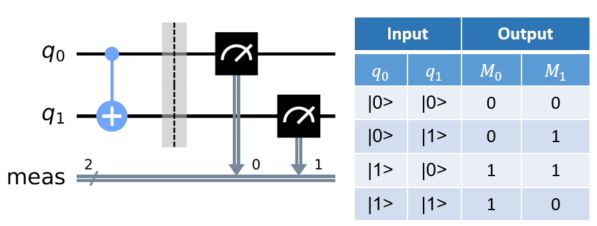
In fig. 10, $M_{0}$ is the measurement outcome on $q_{0}$, and $M_{1}$ is the measurement outcome on $q_{1}$. If we omit the $M_{0}$ column, then we recover the truth table for the classical XOR gate. Note however that this truth table does not include the continuum of possible superpositions of qubit states, which are valid inputs in the analogous quantum gate. Additionally, the $q_{1}$ qubit is still present at the end of the circuit which, for unitary gates, allows for reversibility and reconstruction of the input states given the output and operation applied. Graphically, gates are applied sequentially from left to right, as depicted in fig. 11.

Figure 11: Simple quantum circuit example

There are some gates that operate on larger numbers of qubits. They can be generically represented graphically by rectangles that cover multiple qubit lines, however some specific multi-qubit gates have their own representations. Any unitary single qubit operation can be turned into a controlled operation that depends on the state of another qubit. This is shown by the appropriate box/symbol on the qubit to be operated on, with a vertical line extending from the box to the horizontal line of the controlling qubit with a dot placed at their intersection.

Another contrast to classical logic circuits is that in quantum circuits, one measurement is not enough to deduce the quantum state of the output qubit(s). For example, a qubit in the superposition state

$$|q\rangle=\frac{1}{\sqrt{2}}|0\rangle+\frac{1}{\sqrt{2}}|1\rangle=\begin{bmatrix}\frac{1}{\sqrt{2}}\\ \frac{1}{\sqrt{2}}\end{bmatrix}$$ (85)

has a measurement outcome of 0 with probability $1/2$ and a measurement outcome of 1 with probability $1/2$. Thus several measurements of the same qubit must be made in order to deduce hat it is in the given superposition state. Thus the expectation value is estimated by repeating the measurement many times. Also, since the measurement value only returns the magnitude, the expectation value will be equivalent for a set of quantum states that have the same magnitude but different phase, for example the state

$$|q\rangle=\frac{1}{\sqrt{2}}|0\rangle-\frac{1}{\sqrt{2}}|1\rangle=\begin{bmatrix}\frac{1}{\sqrt{2}}\\ -\frac{1}{\sqrt{2}}\end{bmatrix}$$ (86)

These two states are identical except for a phase factor, and this type of measurement protocol (with a single Z measurement) does not have the resolution to discern between such states. There are workarounds, for example measuring with respect to the x-axis instead of the z-axis, but this leads to extra care that is necessary in designing quantum circuits. For further reading on the fundamentals quantum gates and quantum information, see references [17, 18].

4.2 Embedding Classical Data in Quantum Circuits

Since quantum data and classical data are inherently different in nature, methods must be used to encode classical data in a way that is usable in quantum circuits. Currently, there are two main strategies for building quantum machine learning circuits that use classical data. The first strategy is to use classical dimensionality reduction techniques to reduce the dimension of the classical data to match the number of qubits available in the circuit, such as principle component analysis. In order to embed binary data specifically, an additional step is necessary to convert the reduced dimension data to binary values. An example of a method to reduce dimensionality and convert to binary values is shown in section A1.

Another type of encoding is often called gate encoding. In this paradigm the original floating point data is encoded directly into a quantum circuit with the use of rotation gates. For this type of encoding, the original data is normalized to be in the range of $[0,\pi]$. This range is used to ensure that large and small values are not unintentionally confused for being close together, as they could be if the full $[0,2\pi)$ range was used. In cases where the data has fewer or the same dimensions as the number of qubits, each value of the original data can be directly encoded into the rotation parameter of a rotation gate. In this setup each dimension of the data is encoded by exactly one rotation gate per qubit during the encoding, which can then be used by additional circuit elements for machine learning.

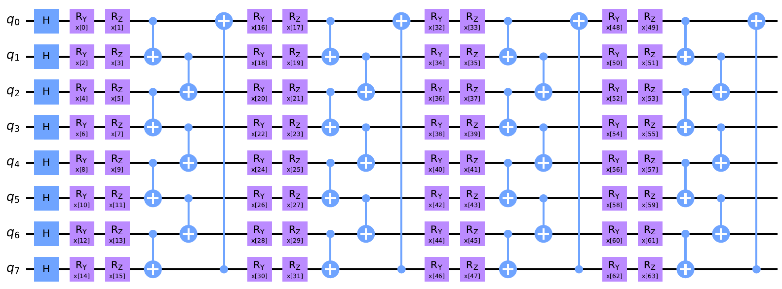
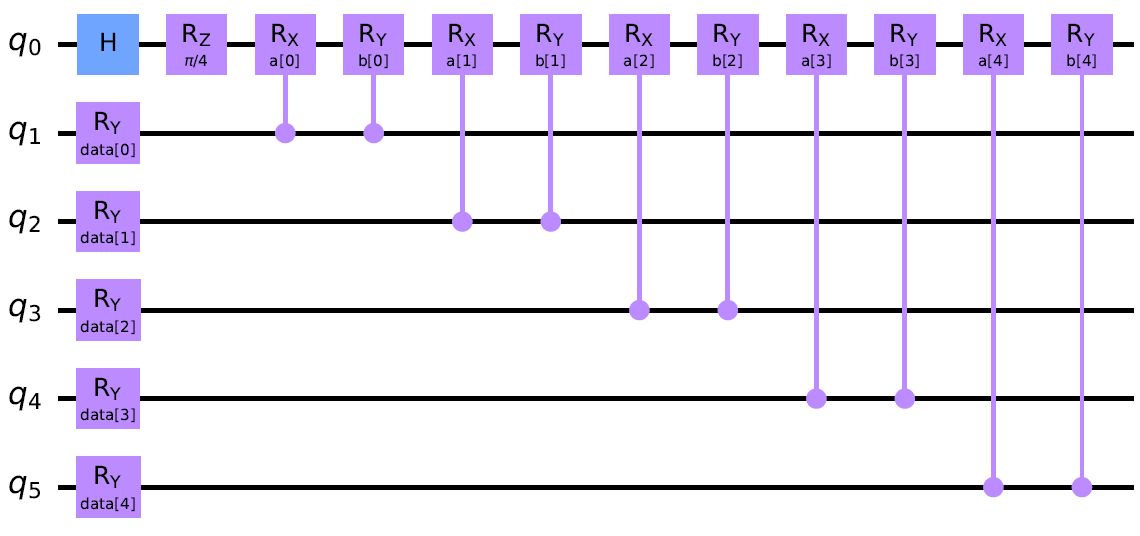
An extension of this method, called block encoding, takes this method and applies it to higher dimensional data. Here the data is represented as a quantum circuit containing many rotation gates applied to the same qubits in order to generate a unique encoding for each data point. Four numbers are important for the design of this encoding scheme: the dimensionality of the data ($D$), the number of qubits ($Q$), the number of layers of the circuit ($L$), and the number of gates per block ($G$). The values of $D$ and $Q$ should already be known and the values of $L$ and $G$ are design variables. To select the values of $L$ and $G$ follow the rule that $D\leq QLG$ while also trying to minimize the product $QLG$. For example, if the data consists of 192 total dimensions, and we are using a quantum computer/simulator with 16 qubits, we can set $L$ to 4 and $G$ to 3. With the design settled, the circuit can be created

The circuit will consist of creating blocks of sets of cycling rotation gates (i.e. an x rotation gate followed by a z rotation gate followed by another x rotation gate). Consecutive rotation gates must be around different axes. The circuit is created by stacking these blocks together evenly across all qubits. After a layer of blocks is created a series of CNOT gates are used to connect consecutive qubit pairs. This process is repeated $L$ times. The rotation amount is defined by the data itself as was done with the gate encoding above. If there are more gates than data dimensions the excess rotation gates use 0 for the rotation angle, so they act as pass through gates. The outputs from this encoding circuit now encode the full data and return unique values for each of the inputs, without needing to follow a complicated dimensionality reduction technique. An example of a circuit with eight qubits, four layers, and two gates per block is shown in fig. 12.

Figure 12: Example of the block encoding method

4.3 Quantum Machine Learning

Quantum machine learning is a new and emerging sub-field of quantum computing that combines two specialized fields into one. The overall process of quantum machine learning is actually very similar to machine learning on classical computers, since quantum machine learning is really a hybrid quantum-classical computation [31]. In quantum machine learning a few key components of the classical machine learning process are replaced by the output of a quantum computer. Most importantly, the error function to be optimized is at least partially calculated by a quantum computer. At least one expectation value of a qubit of a quantum circuit is used to compose the error function [32], though classical components may be included as well, which in some cases increases the functionality. For example, in a classification problem the correct label will be a purely classical value, while the label predicted by the network is calculated on a quantum computer. Also in order to be able to tune and train the quantum network, the network must include some classical parameters that can be kept track of and updated by the algorithm [31, 32].

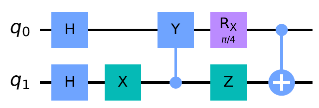
Once the data has been encoded into the quantum circuit using one of the encoding methods mentioned, multi-qubit operations are applied to the data qubits and the readout qubits with the goal of manipulating the readout qubits to some desired state corresponding to the data input. Typically these operations are parametrized controlled rotation gates applied to the readout qubit and controlled off of the data qubits, though non-controlled gates can also be applied to the readout qubit. Upon running the circuit multiple times, the expectation value of the measured readout qubit is used as the final output of the circuit and used to compute a loss function. An example circuit for quantum machine learning is shown in fig. 13. This example used the single rotation gate data encoding method mentioned above.

Figure 13: Example quantum machine learning circuit

In this setup, qubit 0 is the readout qubit and the only one that is measured for the output. The first two gates acting on qubit 0 place the qubit into an unbiased initial state before the network operations are applied. Qubits 1-5 are the data qubits. Each rotation operation on each of those qubits is parameterized by some classical value based on the input data. The remaining gates on qubit 0 are trainable rotation gates controlled by the state of the data qubits. The network gates are parameterized by the trainable network variables $a[1],b[1],a[2],b[2],\dots,a[n],b[n]$.

Similar to classical machine learning, the most common method used to find the optimal parameter values in quantum machine learning is a variant of gradient descent [31]. Since at least part of the error function is calculated on a quantum computer, the gradient calculation also requires partial computation on a quantum computer, which leads to another major difference between classical and quantum machine learning. In classical machine learning fast gradient calculation is enabled by backpropagation. Backpropagation requires intermediate results to be measured/calculated and stored for later use to avoid recalculating them many times. Obtaining intermediate results in the calculation on a quantum computer would require intermediate measurements. However, on a quantum computer these intermediate measurements would destroy any quantum behavior being utilized by the quantum computer. This means that in order to maintain any true quantum calculation, backpropagation is not possible [31, 33] and other methods must be used for calculating the gradient on quantum computers [33]. Fortunately, other methods of calculating the gradient called parameter-shift rules have been developed and fit very well into the architecture of quantum computing.

4.4 Parameter-Shift Rule

The parameter-shift rule is a very useful tool that allows for an analytically exact gradient calculation that can be performed on a quantum computer using the same circuit used to calculate the loss, but with shifted parameter values [33, 34]. In practice, this results in an approximate gradient due to the approximation of the expectation value. This is also the case in the classical machine learning context defined above, however in that case we defined the loss is the finite approximation (under finite data) to the true expectation value. However, in the quantum machine learning context, there are in effect two expectations: an expectation with respect to measurement outcomes and an expectation over the data. In contrast to the finite data problem, expectation values over measurement outcomes can be run as many times as necessary to give sufficient precision.

To show the derivation of this rule, a generic loss function in the form of an expectation value from a readout qubit will be used. Let the loss function $C(\theta)$ be defined as an expectation value [33, 34, 35]:

$$C(\theta):=\langle\psi|\hat{U}_{G}^{\dagger}(\theta)\hat{A}\hat{U}_{G}(\theta)|\psi\rangle$$ (87)

where $|\psi\rangle$ is the vector representing the quantum state and $\langle\psi|$ is its complex conjugate transpose, $\hat{U}_{G}(\theta)$ is a unitary operator parameterized by $\theta$ with the form $\hat{U}_{G}(\theta)=e^{ia\theta\hat{G}}$, where $\hat{G}$ is a Pauli operator, $\hat{U}_{G}^{\dagger}(\theta)$ is the complex conjugate transpose of $\hat{U}_{G}(\theta)$, $\hat{A}$ is the observable being measured, and $a$ is a fixed constant. Taking the derivative with respect to the parameter $\theta$

$$\frac{{\mathrm{d}}C(\theta)}{{\mathrm{d}}\theta}=\frac{{\mathrm{d}}}{{\mathrm{d}}\theta}\langle\psi|\hat{U}_{G}^{\dagger}(\theta)\hat{A}\hat{U}_{G}(\theta)|\psi\rangle$$ (88)

requires the use of the product rule, giving:

$$\frac{{\mathrm{d}}C(\theta)}{{\mathrm{d}}\theta} =\langle\psi|\frac{{\mathrm{d}}}{{\mathrm{d}}\theta}\big{(}\hat{U}_{G}^{\dagger}(\theta)\big{)}\hat{A}\hat{U}_{G}(\theta)|\psi\rangle+\langle\psi|\hat{U}_{G}^{\dagger}(\theta)\hat{A}\frac{{\mathrm{d}}}{{\mathrm{d}}\theta}\big{(}\hat{U}_{G}(\theta)\big{)}|\psi\rangle$$ (89)

$$=\langle\psi|(ia\hat{G})\hat{U}_{G}^{\dagger}(\theta)\hat{A}\hat{U}_{G}(\theta)|\psi\rangle+\langle\psi|\hat{U}_{G}^{\dagger}(\theta)\hat{A}\hat{U}_{G}(\theta)(-ia\hat{G})|\psi\rangle$$ (90)

$$=ia\Big{(}\langle\psi|\hat{G}\hat{U}_{G}^{\dagger}(\theta)\hat{A}\hat{U}_{G}(\theta)|\psi\rangle-\langle\psi|\hat{U}_{G}^{\dagger}(\theta)\hat{A}\hat{U}_{G}(\theta)\hat{G}|\psi\rangle\Big{)}$$ (91)

$$=ia\langle\psi|\hat{U}_{G}^{\dagger}(\theta)\big{[}\hat{G},\hat{A}\big{]}\hat{U}_{G}(\theta)|\psi\rangle$$ (92)

where $\big{[}\hat{G},\hat{A}\big{]}$ is the commutator $\hat{G}\hat{A}-\hat{A}\hat{G}$. While having a commutator in the calculation seems to complicate things, it does allow for the following identity to be used [34, 35, 36]:

$$\big{[}\hat{G},\hat{A}\big{]}=-i\bigg{(}\hat{U}_{G}^{\dagger}\Big{(}\frac{\pi}{2}\Big{)}\hat{A}\hat{U}_{G}\Big{(}\frac{\pi}{2}\Big{)}-\hat{U}_{G}^{\dagger}\Big{(}\frac{\pi}{2}\Big{)}\hat{A}\hat{U}_{G}\Big{(}\frac{\pi}{2}\Big{)}\bigg{)},$$ (93)

where $\hat{U}_{G}(\theta)=e^{ia\theta\hat{G}}$, and $\hat{G}$ is assumed to be some Pauli operator. Using this identity does limit the application of the final result to be valid only with Pauli operator-based unitary gates; but with how commonly used Pauli gates are, this result is still applicable. For a proof of this identity, see section A2.

Applying this identity to the commutator in eq. 92 leads to a form more compatible with quantum circuits:

$$\frac{{\mathrm{d}}C(\theta)}{{\mathrm{d}}\theta} =ia\langle\psi|\hat{U}_{G}^{\dagger}(\theta)(-i)\bigg{(}\hat{U}_{G}^{\dagger}\Big{(}\frac{\pi}{2}\Big{)}\hat{A}\hat{U}_{G}\Big{(}\frac{\pi}{2}\Big{)}-\hat{U}_{G}^{\dagger}\Big{(}\frac{\pi}{2}\Big{)}\hat{A}\hat{U}_{G}\Big{(}\frac{\pi}{2}\Big{)}\bigg{)}\hat{U}_{G}(\theta)|\psi\rangle$$ (94)

$$=a\bigg{(}\langle\psi|\hat{U}_{G}^{\dagger}(\theta)\hat{U}_{G}^{\dagger}\Big{(}\frac{\pi}{2}\Big{)}\hat{A}\hat{U}_{G}\Big{(}\frac{\pi}{2}\Big{)}\hat{U}_{G}(\theta)|\psi\rangle-\langle\psi|\hat{U}_{G}^{\dagger}(\theta)\hat{U}_{G}^{\dagger}\Big{(}-\frac{\pi}{2}\Big{)}\hat{A}\hat{U}_{G}\Big{(}-\frac{\pi}{2}\Big{)}\hat{U}_{G}(\theta)|\psi\rangle\bigg{)}$$ (95)

$$=a\bigg{(}\langle\psi|\hat{U}_{G}^{\dagger}\Big{(}\theta+\frac{\pi}{2}\Big{)}\hat{A}\hat{U}_{G}\Big{(}\theta+\frac{\pi}{2}\Big{)}|\psi\rangle-\langle\psi|\hat{U}_{G}^{\dagger}\Big{(}\theta-\frac{\pi}{2}\Big{)}\hat{A}\hat{U}_{G}\Big{(}\theta-\frac{\pi}{2}\Big{)}|\psi\rangle\bigg{)}$$ (96)

In this form, each term is an expectation value so it can be calculated by a quantum circuit. Of even more importance to this application is that each term is in the same form as the original loss function $C(\theta)$ except for the shift by $\pm\pi/2$. This means the gradient calculation can utilize the exact same circuit as the original loss function. For each parameter’s gradient calculation all that is required is running the circuit twice more, once with the parameter shifted up by $\pi/2$, and once with the parameter shifted down by $\pi/2$ [34]. Using the circuit given in fig. 13 as an example, to calculate the gradient for the first gate parameter, $a[0]$, and letting $k=\pi/2$, the circuits in fig. 14 would both be run and the output measured for each circuit.

Figure 14: Example circuits for parameter upshift (top) and downshift (bottom) on parameter $a[1]$

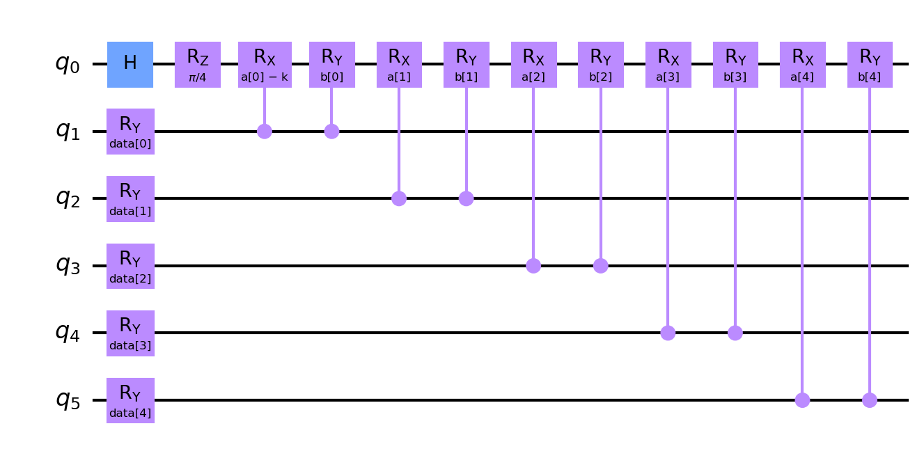
The difference between the outputs of the two circuits in fig. 14 and the factor of $a$ can be calculated classically in the hybrid quantum-classical scheme, which will then give the gradient necessary for gradient descent optimization without requiring intermediate measurements nor interrupting the quantum behavior of the quantum computer. The gradient calculation process is repeated for every network parameter, and the parameters are updated according to the gradient result. With a way to efficiently calculate gradients on a quantum computer, the overall quantum machine learning process can be described by algorithm 2.

The derivation in this section pertains to gates of the form $\hat{U}_{G}(\theta)=e^{ia\theta\hat{G}}$ with $\hat{G}$ a Pauli operator. This is fairly general, however there are cases of gates which do not have this operator structure. In such cases, the stochastic parameter-shift rule generalizes the gradient calculation to operators of any form, including multi-qubit gates [37]. The interested reader may refer to section A6 for a complete derivation.

While the parameter-shift rule does calculate exact gradients, it suffers from requiring significantly more circuit evaluations than classical gradient descent. Similarly, the stochastic parameter-shift rule also requires multiple circuit evaluations per training iteration. While these methods are very popular methods, they are not the only means of training variational quantum circuits. Other notable algorithms include the Simultaneous Perturbation Stochastic Approximation (SPSA) [38] and the Quantum Natural Gradient (QNG) [39].

Algorithm 2 Mini-batch gradient descent algorithm

Training data ${\bf X}_{i},\dots,{\bf X}_{m}$, training labels ${\bf y}$, learning rate $r$, shift $k$

Randomly initialize model parameters $w_{1},\dots,w_{n}$

for $i=1,\dots,m$ do

     Run circuit with parameters ${\bf w}=[w_{1},\dots,w_{n}]$ and calculate the expectation value of the output $\langle\hat{A}({\bf X}_{i},{\bf w})\rangle$

     Calculate loss using data label and circuit output $C({\bf y}_{i},{\bf X}_{i},{\bf w})={\bf y}_{i}-\langle\hat{A}({\bf X}_{i},{\bf w})\rangle$

     for $j=1,\dots,n$ do

         Upshift $j^{th}$ parameter: ${\bf w}_{+}=[w_{1},\dots,w_{j}+k,\dots,w_{n}]$

         Run circuit with new parameter set ${\bf w}_{+}$ and measure output $\text{upshift}=\langle\hat{A}({\bf X}_{i},{\bf w}_{+})\rangle$

         Downshift $j^{th}$ parameter: ${\bf w}_{-}=[w_{1},\dots,w_{j}-k,\dots,w_{n}]$

         Run circuit with new parameter set ${\bf w}_{-}$ and measure output $\text{downshift}=\langle\hat{A}({\bf X}_{i},{\bf w}_{-})\rangle$

         Calculate gradient with respect to $j^{th}$ parameter $\nabla_{w_{j}}C({\bf y}_{i},{\bf X}_{i},{\bf w})=\frac{1}{a}(\text{upshift}-\text{downshift})$

     end for

     Update parameter $w_{j}=w_{j}-r\nabla_{w_{j}}C({\bf y}_{i},{\bf X}_{i},{\bf w})$

end for

return ${\bf w}$

4.5 Variational Quantum Circuit Classification Example – The XOR Problem

The exclusive-or (XOR) problem was discussed earlier in the introduction to artificial neural networks. The problem consists of two classes of data on a grid separated into four blocks, where blocks diagonal from each other contain points in the same class, as depicted in fig. 5. This results in a classification problem where the two classes are not linearly separable. Comparing and contrasting the classical and quantum solutions highlights some of the advantages of quantum computing. Due to the non-linear separation between classes, a classical neural network requires multiple perceptrons to solve the XOR problem. However, it has been shown that a simple quantum circuit, shown in fig. 15, using only one qubit as a single perceptron can solve the XOR problem. This approach leverages the phase of the qubit as an extra degree of freedom [40].

Figure 15: Quantum circuit to solve the XOR problem

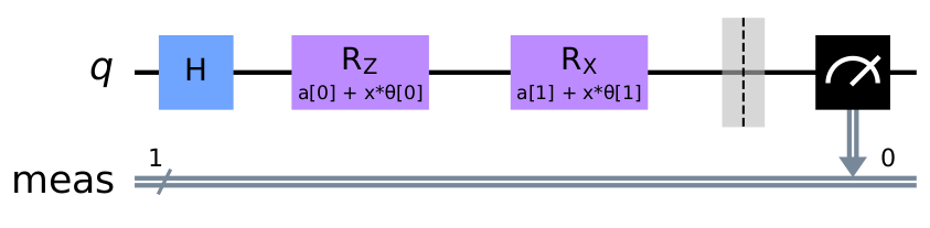
This circuit is fairly simple and consists of only three gates, a Hadamard gate followed by a $Z$- rotation gate, and then an $X$-rotation gate. The rotation angles of the gates are determined by the following classical expressions [40]:

$$\text{Z-rotation angle: }\theta_{1}x_{1}+\alpha$$ (97)

$$\text{X-rotation angle: }\theta_{2}x_{2}+\alpha,$$ (98)

where $\theta_{1},\theta_{2}$ are trainable parameters, $x_{1},x_{2}$ are the input values, and $\alpha$ is another trainable parameter. Here there is a direct solution by using $\theta_{1}=\theta_{2}=\pi$ and $\alpha=-\pi/2$ [40], however this circuit could be trained by gradient descent. Indeed, for the input vectors $(x_{1},x_{2})=(0,0)$ and $(x_{1},x_{2})=(1,1)$ the circuit gives a result near the zero state (up to quantum hard precision), and for the input vectors $(x_{1},x_{2})=(0,1)$ and $(x_{1},x_{2})=(1,0)$ the circuit gives an output near the one state (up to quantum hard precision) [40]. Finally, with “noisy" non-integer inputs between 0 and 1, the circuit gives output states between the zero state and the one state (see Table 2 in [40]).

Extending the circuit and methods introduced above, nearly identical results are obtained using a quantum machine learning framework and training on a larger data set. To do this, the circuit from [40] is modified to make it more compatible with the parameter-shift gradient descent method described earlier. This modified circuit is shown below in fig. 16.

Figure 16: Modified circuit for learning to solve the XOR problem.

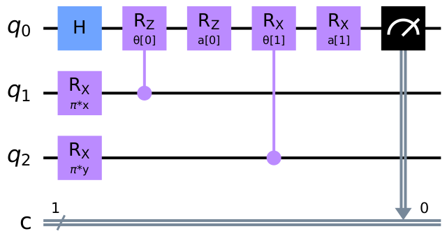
This circuit adds two qubits so that the rotation data embedding scheme can be used. The $CRZ(\theta_{1})$ gate controlled on qubit 1 for the first data input corresponds to the $\theta_{1}x_{1}$ part of the input parameters to the original $Z$ rotation gate, and similarly for $CRX(\theta_{2})$ and $\theta_{2}x_{2}$. Since originally the $\alpha$ parameter is added as a constant, it can be applied in the new circuit as another gate applied in series with the respective controlled gate. Additionally, the single $\alpha$ parameter has been split into $\alpha_{1}$ and $\alpha_{2}$ for the Z and X rotations, respectively, to allow the circuit to be more flexible.

The data for training and testing this new circuit is generated from a random uniform distribution between 0 and 1 for the $x$ and $y$ values of each data point, though values of exactly 0.5 were excluded as they would be on the class boundary and degenerate. 1000 sample points were generated, with 750 being used for training, 63 used for validation during training, and 187 used for blind testing after training was complete. This dataset is shown in fig. 17.

Figure 17: Generated XOR dataset.

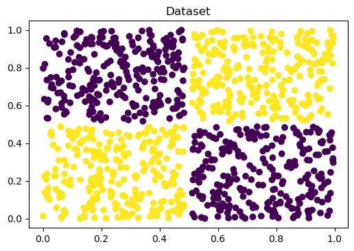
The yellow data points are assigned to class 0, corresponding to a zero state output of the read-out qubit, and the purple data points are assigned to class 1, corresponding to a one state output of the read-out qubit. The observable used is the Pauli $Z$ gate, which has two possible eigenvalues $\{+1,-1\}$, which are used as the labels for the classes, respectively. The goal for the network is to rotate the read-out qubit towards the zero state for data from class 0, and towards the one state for data from class 1. The expectation value should be closer to +1 for inputs from class 0, and closer to -1 for inputs from class 1. The loss function to be optimized is given by the mean squared error of the expectation value.

To optimize the loss function, mini-batch gradient descent optimization was used, with a batch size of 25 data samples and a learning rate (or step size) of 0.025. The network was trained over 150 epochs. The loss function was averaged over the 25 samples in each mini-batch and that average loss function was used in the gradient calculation. The gradient was calculated using the parameter-shift rule in eq. 96. To classify a sample in the validation and testing phases of the machine learning process, the continuously valued expectation value output from the network is thresholded. Outputs greater than or equal to are classified as class 0 and outputs less than are classified as class 1.

Using these methods, the network was successfully trained and the results found match the results given in [40]. The loss was recorded for every batch, and the plot of the loss vs. batch is shown below in LABEL:fig:xor_training_loss. The loss decreased to less than 0.5 on average, and plateaued fairly early in the training process. The plot of validation accuracy per batch over the training period also plateaued early in training as well, as shown in LABEL:fig:xor_valid_accuracy. The validation accuracy converges to 100% after about 1000 batches, which is an indicator of good network performance. In testing the network performed very well, correctly classifying 100% of the testing data samples. The true labels and the classification results from the network on the test set are shown in LABEL:fig:xor_true_and_pred_labels. The subplots are identical, showing that the network assigned the true label to every test sample. Furthermore, converged parameters are in full agreement with the parameters used in [40]. The convergence of the parameters over the training period are shown below in LABEL:fig:xor_theta_convergence and LABEL:fig:xor_alpha_convergence, where the ideal parameter values from [40] are shown by dashed lines.

In LABEL:fig:xor_theta_convergence, the dashed lines are at exactly $\pi$, which correspond to the value used for $\theta_{1}$ and $\theta_{2}$ in [40]. The network parameters trained here, shown with solid lines, converge to approximately $\pi$. The final values for $\theta_{1}$ and $\theta_{2}$ at the end of training were $3.14147$ and $3.14479$, respectively. The results for the $\alpha$ parameters are shown in LABEL:fig:xor_alpha_convergence. The dashed lines are at exactly $-\pi/2$, which correspond to the values used for $\alpha_{1}$ and $\alpha_{2}$ in [40]. The network parameters $\alpha_{1}$ and $\alpha_{2}$ converged to values of $4.71247$ and $4.71022$.

At first it appears that the network parameters are not in agreement as they converged to different values, however these values are approximately equal to $+3\pi/2$. Since rotations wrap from $2\pi$ back to 0, a rotation by $+3\pi/2$ is equivalent to a rotation by $-\pi/2$. Thus the circuit trained here is equivalent to the circuit presented in [40]. These results indicate that quantum circuits can be trained (in simulation) using quantum machine learning methods. Since the XOR problem is an example of a problem that can be solved with a single quantum neuron in contrast to a multi-layer classical perceptron, this simulated demonstration highlights some of the potential advantages of quantum computing and quantum machine learning.

5 Conclusion

This manuscript introduces the relevant concepts of quantum machine learning, and serves as introductory material. The basic notions of quantum mechanics are described, including quantum phase, superposition, entanglement, and expectations. These are used to introduce quantum gates as fundamental building blocks of the quantum computing framework in comparison with the classical digital logic framework. The basics of classical machine learning are introduced specifically related to deep learning for classification, and are used as a background in order to introduce standard notions in quantum machine learning. Finally these notions are applied to an example problem that highlights some potential advantages of quantum machine learning over its classical counterpart. With the growing capabilities of quantum computers, quantum machine learning holds promise for solving hard problems in a variety of domains, and warrants further investigation into the quantum advantage of quantum machine learning.

Appendix

A1 Binary Dimensionality Reduction Example

In this example we will assume that our data has a starting dimension of 200 and that we are using a quantum computer/simulator that has 16 qubits. For this example we will assume that we are embedding binary values. To convert the high dimensional floating point data to a 16 bit binary vector, an ensemble of weak classifiers will be used.

For the weak classifier, the perceptron mentioned in the main document is used. This works well in the ensemble case as the algorithm can be optimized through direct optimization via

$${\bf w}={\bf y}{\bf X}^{\mathsf{T}}({\bf X}{\bf X}^{\mathsf{T}})^{-1},$$ (A1)

where ${\bf y}\in\{-1,1\}$ is the vector of true labels and ${\bf X}$ is the set of all training data. This is the solution to solving the equation ${\bf y}={\bf w}{\bf X}$ for ${\bf w}$.

To train an ensemble of perceptrons the training data is split into $N$ sets of equal size, where $N$ is the number of desired bits in the quantum encoding. A perceptron is then trained, using eq. A1, for each of the $N$ sets. The entirety of the data is then passed through each of the $N$ perceptrons. Each $-1$ is converted to zero, and the $N$ outputs are combined together to form the binary representation for the algorithm comparisons.

A2 Statement and Proof of the Pauli Commutator Identity

Let $\sigma_{i}$ be a Pauli matrix, and $B$ any operator. Let $U_{i}(\theta):=\exp(-i\frac{\theta}{2}\sigma_{i})$. Then

$$[\sigma_{i},B]=-i\bigg{(}U_{i}^{\dagger}\Big{(}\frac{\pi}{2}\Big{)}BU_{i}\Big{(}\frac{\pi}{2}\Big{)}-U_{i}^{\dagger}\Big{(}-\frac{\pi}{2}\Big{)}BU_{i}\Big{(}-\frac{\pi}{2}\Big{)}\bigg{)}$$ (A2)

Proof.

First, note that for Pauli matrix $\sigma_{i}$, $i=1,2,3$, $\sigma_{i}^{\dagger}=\sigma_{i}$ (that is, Pauli matrices are Hermitian). Plugging in the definition of $U_{i}(\frac{\pi}{2})$ yields

$$[\sigma_{i},B]=-i\bigg{(}\exp\Big{(}i\frac{\pi}{4}\sigma_{i}\Big{)}B\exp\Big{(}-i\frac{\pi}{4}\sigma_{i}\Big{)}-\exp\Big{(}-i\frac{\pi}{4}\sigma_{i}\Big{)}B\exp\Big{(}i\frac{\pi}{4}\sigma_{i}\Big{)}\bigg{)}.$$ (A3)

next, we apply the following Pauli matrix identity:

$$e^{ia(\hat{n}\cdot\vec{\sigma})}=I\cos a+i(\hat{n}\cdot\vec{\sigma})\sin a,\quad|\hat{n}|=1,$$ (A4)

where $\vec{\sigma}=\sigma_{x}\hat{x}+\sigma_{y}\hat{y}+\sigma_{z}\hat{z}$. Put simply, this intermediate identity holds through the expansion of the exponential into an infinite sum, splitting the sum into even and odd exponent parts, and noting that $\sigma_{i}^{2p}=I$, $p\in\mathbb{N}_{+}$, which causes the cosine (composed of the even exponent terms) to only have prefactor Identity, and the sine (composed of the odd exponent terms) to be left with the Pauli matrix prefactor. In our case, $\sigma_{i}=\hat{n}_{i}\cdot\vec{\sigma}$, thus

$$\exp\Big{(}i\frac{\pi}{4}\sigma_{i}\Big{)}=I\cos\frac{\pi}{4}+i\sigma_{i}\sin\frac{\pi}{4}$$ (A5)

Applying this identity, and also the fact that $\cos(-a)=\cos(a)$ and $\sin(-a)=-\sin(a)$, yields

$$[\sigma_{i},B] =-i\bigg{(}\Big{(}I\cos\frac{\pi}{4}+i\sigma_{i}\sin\frac{\pi}{4}\Big{)}B\Big{(}I\cos\frac{-\pi}{4}+i\sigma_{i}\sin\frac{-\pi}{4}\Big{)}$$

$$\qquad\quad-\Big{(}I\cos\frac{-\pi}{4}+i\sigma_{i}\sin\frac{-\pi}{4}\Big{)}B\Big{(}I\cos\frac{\pi}{4}+i\sigma_{i}\sin\frac{\pi}{4}\Big{)}\bigg{)}$$ (A6)

$$=-i\bigg{(}\Big{(}I\cos\frac{\pi}{4}+i\sigma_{i}\sin\frac{\pi}{4}\Big{)}B\Big{(}I\cos\frac{\pi}{4}-i\sigma_{i}\sin\frac{\pi}{4}\Big{)}$$

$$\qquad\quad-\Big{(}I\cos\frac{\pi}{4}-i\sigma_{i}\sin\frac{\pi}{4}\Big{)}B\Big{(}I\cos\frac{\pi}{4}+i\sigma_{i}\sin\frac{\pi}{4}\Big{)}\bigg{)}$$ (A7)

$$=-i\bigg{(}\Big{(}I\frac{\sqrt{2}}{2}+i\sigma_{i}\frac{\sqrt{2}}{2}\Big{)}B\Big{(}I\frac{\sqrt{2}}{2}-i\sigma_{i}\frac{\sqrt{2}}{2}\Big{)}-\Big{(}I\frac{\sqrt{2}}{2}-i\sigma_{i}\frac{\sqrt{2}}{2}\Big{)}B\Big{(}I\frac{\sqrt{2}}{2}+i\sigma_{i}\frac{\sqrt{2}}{2}\Big{)}\bigg{)}$$ (A8)

$$=-\frac{i}{2}\bigg{(}B-iB\sigma_{i}+i\sigma_{i}B-i^{2}\sigma_{i}B\sigma_{i}-\Big{(}B+iB\sigma_{i}-i\sigma_{i}B-i^{2}\sigma_{i}B\sigma_{i}\Big{)}\bigg{)}$$ (A9)

$$=-\frac{i}{2}\bigg{(}-2iB\sigma_{i}+2i\sigma_{i}B\bigg{)}=\sigma_{i}B-B\sigma_{i}$$ (A10)

∎

A3 Derivation of the Baker-Campbell-Hausdorff Identity

Let $\hat{A}:{\cal H}\rightarrow{\cal H}$ and $\hat{B}:{\cal H}\rightarrow{\cal H}$ be operators in Hilbert space ${\cal H}$, and let $f(\lambda)$ be a single parameter function with $\lambda\in\mathbb{C}$, defined by:

$$f(\lambda)=e^{\lambda\hat{A}}\hat{B}e^{-\lambda\hat{A}}.$$ (A11)

Then

$$f(\lambda)=e^{\lambda[\hat{A},\cdot]}\hat{B}.$$ (A12)

Proof.

Starting with the function $f(\lambda)=e^{\lambda\hat{A}}\hat{B}e^{-\lambda\hat{A}}$, which a typical form of an expectation value in the Heisenberg or Interaction picture, write it as a Taylor series expansion of the form:

$$F(x)=\sum_{n=0}^{\infty}\frac{F^{n}(a)(x-a)^{n}}{n!}.$$ (A13)

Taking the first derivative of $f(\lambda)$ yields:

$$f^{\prime}(\lambda)=e^{\lambda\hat{A}}\hat{A}\hat{B}e^{-\lambda\hat{A}}-e^{\lambda\hat{A}}\hat{B}\hat{A}e^{-\lambda\hat{A}}=e^{\lambda\hat{A}}[\hat{A},\hat{B}]e^{-\lambda\hat{A}}.$$ (A14)

The evaluating for $\lambda=0$:

$$f^{\prime}(0)=e^{0\hat{A}}[\hat{A},\hat{B}]e^{-0\hat{A}}=[\hat{A},\hat{B}]=[\hat{A},\cdot]^{1}\hat{B}$$ (A15)

where $[\hat{A},\cdot]^{1}\hat{B}$ is an alternative notation whose usefulness will become apparent shortly. Repeating the above steps for the second derivative gives:

$$f^{\prime\prime}(\lambda) =e^{\lambda\hat{A}}\hat{A}[\hat{A},\hat{B}]e^{-\lambda\hat{A}}-e^{\lambda\hat{A}}[\hat{A},\hat{B}]\hat{A}e^{-\lambda\hat{A}}=e^{\lambda\hat{A}}\big{[}\hat{A},[\hat{A},\hat{B}]\big{]}e^{-\lambda\hat{A}}=e^{\lambda\hat{A}}[\hat{A},\cdot]^{2}\hat{B}e^{-\lambda\hat{A}}$$ (A16)

$$f^{\prime\prime}(0) =e^{0\hat{A}}\big{[}\hat{A},[\hat{A},\hat{B}]\big{]}e^{-0\hat{A}}=\big{[}\hat{A},[\hat{A},\hat{B}]\big{]}=[\hat{A},\cdot]^{2}\hat{B}$$ (A17)

Using the developing pattern, the $n^{th}$ derivative evaluated at zero can be written as:

$$f^{n}(0)=[\hat{A},\cdot]^{n}\hat{B}.$$ (A18)

Now, writing $f(\lambda)$ as a Taylor expansion eq. A13 centered at zero (i.e. with $a=0$) gives:

$$f(\lambda)=e^{\lambda\hat{A}}\hat{B}e^{-\lambda\hat{A}}=\sum_{n=0}^{\infty}\frac{f^{n}(0)(\lambda-0)^{n}}{n!}=\sum_{n=0}^{\infty}\frac{[\hat{A},\cdot]^{n}\hat{B}\lambda^{n}}{n!}.$$ (A19)

The final form of the expression looks like the definition of an exponential,

$$e^{\lambda\hat{A}}=\sum_{n=0}^{\infty}\frac{\lambda^{n}\hat{A}^{n}}{n!}.$$ (A20)

Rewriting $f(\lambda)$ in exponential form yields:

$$f(\lambda)=e^{\lambda\hat{A}}\hat{B}e^{-\lambda\hat{A}}=\sum_{n=0}^{\infty}\frac{[\hat{A},\cdot]^{n}\hat{B}\lambda^{n}}{n!}=\left(\sum_{n=0}^{\infty}\frac{\lambda^{n}[\hat{A},\cdot]^{n}}{n!}\right)\hat{B}=e^{\lambda[\hat{A},\cdot]}\hat{B},$$ (A21)

which is the Baker-Campbell-Hausdorff identity. ∎

A4 Derivation of the Derivative of a Parametric Exponential Operator

Let $Z(\theta)$ be a some operator parameterized by $\theta$. Then

$$\frac{\partial}{\partial\theta}e^{Z(\theta)}=\int_{0}^{1}e^{(1-s)Z(\theta)}\frac{\partial}{\partial\theta}Z(\theta)e^{sZ(\theta)}{\mathrm{d}}s$$ (A22)

Proof.

First, note that $e^{Z(\theta)}=\sum_{n=0}^{\infty}\frac{Z(\theta)^{n}}{n!}$. So

$$\frac{\partial}{\partial\theta}e^{Z(\theta)} =\sum_{n=0}^{\infty}\frac{1}{n!}\frac{\partial}{\partial\theta}Z(\theta)^{n}$$ (A23)

$$=\frac{\partial}{\partial\theta}\Big{(}I+Z(\theta)+\frac{1}{2}Z(\theta)^{2}+\dots\Big{)}$$ (A24)

$$=0+\frac{\partial Z(\theta)}{\partial\theta}+\frac{1}{2}\Big{(}Z(\theta)\frac{\partial Z(\theta)}{\partial\theta}+\frac{\partial Z(\theta)}{\partial\theta}Z(\theta)\Big{)}+$$

$$\quad+\frac{1}{6}\Big{(}\frac{\partial Z(\theta)}{\partial\theta}Z(\theta)^{2}+Z(\theta)\frac{\partial Z(\theta)}{\partial\theta}Z(\theta)+Z(\theta)^{2}\frac{\partial Z(\theta)}{\partial\theta}\Big{)}$$

$$\quad+\frac{1}{24}\Big{(}\frac{\partial Z(\theta)}{\partial\theta}Z(\theta)^{3}+Z(\theta)\frac{\partial Z(\theta)}{\partial\theta}Z(\theta)^{2}+Z(\theta)^{2}\frac{\partial Z(\theta)}{\partial\theta}Z(\theta)+Z(\theta)^{3}\frac{\partial Z(\theta)}{\partial\theta}\Big{)}+\dots$$ (A25)

$$=I\frac{\partial Z(\theta)}{\partial\theta}I+\Big{(}\frac{1}{2}Z(\theta)+\frac{1}{6}Z(\theta)^{2}+\frac{1}{24}Z(\theta)^{3}+\dots\Big{)}\frac{\partial Z(\theta)}{\partial\theta}I$$

$$\quad+I\frac{\partial Z(\theta)}{\partial\theta}\Big{(}\frac{1}{2}Z(\theta)+\frac{1}{6}Z(\theta)^{2}+\frac{1}{24}Z(\theta)^{3}+\dots\Big{)}$$

$$\quad+\Big{(}\frac{1}{24}Z(\theta)^{2}+\dots\Big{)}\frac{\partial Z(\theta)}{\partial\theta}Z(\theta)+Z(\theta)\frac{\partial Z(\theta)}{\partial\theta}\Big{(}\frac{1}{24}Z(\theta)^{2}+\dots\Big{)}+\dots$$ (A26)

$$=\sum_{n=0}^{\infty}\sum_{k=0}^{n}\frac{1}{(n+1)!}Z(\theta)^{k}\frac{\partial Z(\theta)}{\partial\theta}Z(\theta)^{n-k}.$$ (A27)

Now, shifting/swapping the indices using the identity [41]

$$\sum_{n=0}^{\infty}\sum_{k=0}^{n}f_{n,k}=\sum_{k=0}^{\infty}\sum_{n=k}^{\infty}f_{n,k}=\sum_{k=0}^{\infty}\sum_{n=0}^{\infty}f_{n+k,k},$$ (A28)

we have

$$\frac{\partial}{\partial\theta}e^{Z(\theta)}=\sum_{k=0}^{\infty}\sum_{n=0}^{\infty}\frac{1}{(n+k+1)!}Z(\theta)^{k}\frac{\partial Z(\theta)}{\partial\theta}Z(\theta)^{n}.$$ (A29)

Now multiply by $1=\frac{n!k!}{n!k!}$

$$\frac{\partial}{\partial\theta}e^{Z(\theta)}=\sum_{k=0}^{\infty}\sum_{n=0}^{\infty}\frac{n!k!}{n!k!(n+k+1)!}Z(\theta)^{k}\frac{\partial Z(\theta)}{\partial\theta}Z(\theta)^{n}.$$ (A30)

Next, we note that $\frac{n!k!}{(n+k+1)!}$ is the definition of the beta function, which can be represented as an integral via Euler’s beta function identity (proof provided after the conclusion of this proof)

$$B(k+1,n+1):=\frac{n!k!}{(n+k+1)!}=\int_{0}^{1}(1-s)^{k}s^{n}{\mathrm{d}}s$$ (A31)

Plugging in Euler’s beta function identity yields

$$\frac{\partial}{\partial\theta}e^{Z(\theta)} =\int_{0}^{1}\sum_{k=0}^{\infty}\sum_{n=0}^{\infty}\frac{1}{n!k!}\Big{(}(1-s)Z(\theta)\Big{)}^{k}\frac{\partial Z(\theta)}{\partial\theta}\Big{(}sZ(\theta)\Big{)}^{n}{\mathrm{d}}s$$ (A32)

$$=\int_{0}^{1}\sum_{k=0}^{\infty}\frac{1}{k!}\Big{(}(1-s)Z(\theta)\Big{)}^{k}\frac{\partial Z(\theta)}{\partial\theta}\sum_{n=0}^{\infty}\frac{1}{n!}\Big{(}sZ(\theta)\Big{)}^{n}{\mathrm{d}}s$$ (A33)

$$=\int_{0}^{1}e^{(1-s)Z(\theta)}\frac{\partial Z(\theta)}{\partial\theta}e^{sZ(\theta)}{\mathrm{d}}s$$ (A34)

∎

A5 Statement and Proof of Euler’s beta function identity

$$B(k,n):=\frac{(n-1)!(k-1)!}{(n+k-1)!}=\int_{0}^{1}(1-s)^{k-1}s^{n-1}{\mathrm{d}}s$$ (A35)

Proof.

This proof is readily available in numerous online sources. First, by integration-by-parts, one can show that for $m\in\mathbb{N}$,

$$\int_{0}^{\infty}p^{m-1}e^{-p}{\mathrm{d}}p=(m-1)!$$ (A36)

Next, consider the product

$$(m-1)!(n-1)! =\int_{0}^{\infty}p^{m-1}e^{-p}{\mathrm{d}}p\times\int_{0}^{\infty}q^{n-1}e^{-q}{\mathrm{d}}q.$$ (A37)

Rewriting it as a double integral over the region $x,y\geq 0$ in the $(x,y)$-plane yields

$$(m-1)!(n-1)!=2\int_{0}^{\infty}x^{2m-1}e^{-x^{2}}{\mathrm{d}}x\times 2\int_{0}^{\infty}y^{2n-1}e^{-y^{2}}{\mathrm{d}}y.$$ (A38)

Now transform to polar coordinates: $x=r\cos\theta$, $y=r\sin\theta$, and ${\mathrm{d}}x{\mathrm{d}}y=r{\mathrm{d}}r{\mathrm{d}}\theta$

$$(m-1)!(n-1)! =4\int_{0}^{\infty}r^{2(m+n-1)}e^{-r^{2}}r{\mathrm{d}}r\times\int_{0}^{\pi/2}\sin^{2n-1}\theta\cos^{2m-1}\theta{\mathrm{d}}\theta$$ (A39)

$$=2(m+n-1)!\int_{0}^{\pi/2}\sin^{2n-1}\theta\cos^{2m-1}\theta{\mathrm{d}}\theta,$$ (A40)

where we have applied the single integer factorial form in eq. A36. Thus, we have that

$$\frac{(m-1)!(n-1)!}{(m+n-1)!}=2\int_{0}^{\pi/2}\sin^{2n-1}\theta\cos^{2m-1}\theta{\mathrm{d}}\theta.$$ (A41)

Finally, make the change of variable $t=sin^{2}\theta$, which implies that ${\mathrm{d}}t=2\sin\theta\cos\theta{\mathrm{d}}\theta$ and $\cos^{2}\theta=1-t$. Re-writing the integral and applying this change of variables yields

$$2\int_{0}^{\pi/2}\sin^{2n-1}\theta\cos^{2m-1}\theta{\mathrm{d}}\theta =\int_{0}^{\pi/2}\sin^{2n-2}\theta\cos^{2m-2}\theta 2\sin\theta\cos\theta{\mathrm{d}}\theta$$ (A42)

$$=\int_{0}^{1}(1-t)^{n-1}t^{m-1}{\mathrm{d}}t$$ (A43)

Thus we have concluded that

$$\frac{(m-1)!(n-1)!}{(m+n-1)!}=\int_{0}^{1}(1-t)^{n-1}t^{m-1}{\mathrm{d}}t$$ (A44)

∎

A6 Derivation of the Stochastic Parameter-Shift Rule

The stochastic parameter-shift rule allows for a more generalizable gradient calculation that is applicable to a wider variety of gates including multi-qubit gates [37]. This is done by replacing the operator $\hat{G}$ in $\hat{U}_{G}(\theta)=e^{-ia\theta\hat{G}}$ with $\hat{G}=\hat{H}+\theta\hat{V}$, where $\hat{H}$ is an arbitrary linear combination of Pauli operator tensor products, and $\hat{V}$ is a tensor product of Pauli operators. Since multi-qubit operators can be constructed as a sum of tensor products of Pauli operators, the use of $\hat{H}$ and $\hat{V}$ in this form allows for generalization to arbitrary gates and calculation of the gradient analytically. The loss function $C(\theta)$ then becomes:

$$C(\theta)=\langle\psi|\hat{U}_{G}^{\dagger}(\theta)\hat{A}\hat{U}_{G}(\theta)|\psi\rangle=\langle\psi|e^{ia\theta(\hat{H}+\theta\hat{V})}\hat{A}e^{-ia\theta(\hat{H}+\theta\hat{V})}|\psi\rangle.$$ (A45)

To find the gradient of this loss function and manipulate it into a form compatible with quantum computers requires several identities. The Baker-Campbell-Hausdorff (BCH) identity [42] is derived in section A3, and is given by:

$$f(\lambda)=e^{\lambda\hat{A}}\hat{B}e^{-\lambda\hat{A}}=\left(\sum_{n=0}^{\infty}\frac{\lambda^{n}[\hat{A},\cdot]^{n}}{n!}\right)\hat{B}=e^{\lambda[\hat{A},\cdot]}\hat{B}.$$ (A46)

We also apply the commutator identity in eq. 93, and the following exponential derivative rule, derived in section A4 [37, 42]:

$$\frac{\partial e^{\hat{Z}(\theta)}}{\partial\theta}=\int_{0}^{1}e^{(1-s)\hat{Z}(\theta)}\frac{\partial\hat{Z}(\theta)}{\partial\theta}e^{s\hat{Z}(\theta)}{\mathrm{d}}s$$ (A47)

With this, we derive an analytic form of the gradient that may still be evaluated by a quantum computer. The starting point is eq. A45, repeated here for clarity:

$$C(\theta)=\langle\psi|e^{ia\theta(\hat{H}+\theta\hat{V})}\hat{A}e^{-ia\theta(\hat{H}+\theta\hat{V})}|\psi\rangle.$$

Applying the BCH identity eq. A46 yields:

$$C(\theta)=\langle\psi|e^{ia[\hat{H}+\theta\hat{V},\cdot]}\hat{A}|\psi\rangle$$ (A48)

Next, the derivative is taken and passed into the expectation:

$$\frac{{\mathrm{d}}C(\theta)}{{\mathrm{d}}\theta}=\frac{\partial}{\partial\theta}\langle\psi|e^{ia[\hat{H}+\theta\hat{V},\cdot]}\hat{A}|\psi\rangle=\langle\psi|\frac{\partial}{\partial\theta}e^{ia[\hat{H}+\theta\hat{V},\cdot]}\hat{A}|\psi\rangle.$$ (A49)

Next the exponential derivative rule in eq. A47 is applied, where $e^{\hat{Z}(\theta)}=e^{ia[\hat{H}+\theta\hat{V},\cdot]}$ and $\frac{\partial\hat{Z}(\theta)}{\partial\theta}=\frac{\partial}{\partial\theta}ia[\hat{H}+\theta\hat{V},\cdot]=ia[\hat{V},\cdot]$, giving:

$$\frac{{\mathrm{d}}C(\theta)}{{\mathrm{d}}\theta}=\langle\psi|\frac{\partial}{\partial\theta}e^{ia[\hat{H}+\theta\hat{V},\cdot]}\hat{A}|\psi\rangle=\langle\psi|\int_{0}^{1}e^{(1-s)ia[\hat{H}+\theta\hat{V},\cdot]}ia[\hat{V},\cdot]e^{sia[\hat{H}+\theta\hat{V},\cdot]}\hat{A}{\mathrm{d}}s|\psi\rangle.$$ (A50)

Next, the constants are moved out of the inner product and the BCH identity eq. A46 is applied to the term in red:

$$\frac{{\mathrm{d}}C(\theta)}{{\mathrm{d}}\theta} =ia\langle\psi|\int_{0}^{1}e^{(1-s)ia[\hat{H}+\theta\hat{V},\cdot]}ia[\hat{V},\cdot]{\color[rgb]{1,0,0}\{e^{sia[\hat{H}+\theta\hat{V},\cdot]}\hat{A}\}}{\mathrm{d}}s|\psi\rangle$$ (A51)

$$=ia\langle\psi|\int_{0}^{1}e^{(1-s)ia[\hat{H}+\theta\hat{V},\cdot]}ia[\hat{V},\cdot]e^{sia(\hat{H}+\theta\hat{V})}\hat{A}e^{-sia(\hat{H}+\theta\hat{V})}{\mathrm{d}}s|\psi\rangle$$ (A52)

$$=ia\langle\psi|\int_{0}^{1}e^{(1-s)ia[\hat{H}+\theta\hat{V},\cdot]}ia\big{[}\hat{V},e^{sia(\hat{H}+\theta\hat{V})}\hat{A}e^{-sia(\hat{H}+\theta\hat{V})}\big{]}{\mathrm{d}}s|\psi\rangle,$$ (A53)

where we use the commutator notation $[\hat{A},\cdot]\hat{B}=[\hat{A},\hat{B}]$. Since the first term of the commutator now only contains $\hat{V}$, we can now apply the commutator identity eq. 93:

$$\frac{{\mathrm{d}}C(\theta)}{{\mathrm{d}}\theta}=a\langle\psi|\int_{0}^{1}e^{(1-s)ia[\hat{H}+\theta\hat{V},\cdot]}\bigg{(} \hat{U}_{V}^{\dagger}\Big{(}\frac{\pi}{2}\Big{)}e^{sia(\hat{H}+\theta\hat{V})}\hat{A}e^{-sia(\hat{H}+\theta\hat{V})}\hat{U}_{V}\Big{(}\frac{\pi}{2}\Big{)}$$

$$-\hat{U}_{V}^{\dagger}\Big{(}-\frac{\pi}{2}\Big{)}e^{sia(\hat{H}+\theta\hat{V})}\hat{A}e^{-sia(\hat{H}+\theta\hat{V})}\hat{U}_{V}\Big{(}-\frac{\pi}{2}\Big{)}\bigg{)}{\mathrm{d}}s|\psi\rangle,$$ (A54)

where $\hat{U}_{V}(\theta)=e^{ib\theta\hat{V}}$ and $b$ is another constant $b\neq a$. The BCH identity is applied once more to the entire term inside the brackets where

$$\bigg{(}\hat{U}_{V}^{\dagger}\Big{(}\frac{\pi}{2}\Big{)}e^{sia(\hat{H}+\theta\hat{V})}\hat{A}e^{-sia(\hat{H}+\theta\hat{V})}\hat{U}_{V}\Big{(}\frac{\pi}{2}\Big{)}-\hat{U}_{V}^{\dagger}\Big{(}-\frac{\pi}{2}\Big{)}e^{sia(\hat{H}+\theta\hat{V})}\hat{A}e^{-sia(\hat{H}+\theta\hat{V})}\hat{U}_{V}\Big{(}-\frac{\pi}{2}\Big{)}\bigg{)}$$ (A55)

is treated as the matrix $\hat{B}$ in $e^{\lambda\hat{A}}\hat{B}e^{-\lambda\hat{A}}=e^{\lambda[\hat{A},\cdot]}\hat{B}$, and $e^{(1-s)ia[\hat{H}+\theta\hat{V},\cdot]}$ is the exponential. This BCH identity application yields:

$$\frac{{\mathrm{d}}C(\theta)}{{\mathrm{d}}\theta} =a\langle\psi|\int_{0}^{1}e^{(1-s)ia(\hat{H}+\theta\hat{V})}\bigg{(}\hat{U}_{V}^{\dagger}\Big{(}\frac{\pi}{2}\Big{)}e^{sia(\hat{H}+\theta\hat{V})}\hat{A}e^{-sia(\hat{H}+\theta\hat{V})}\hat{U}_{V}\Big{(}\frac{\pi}{2}\Big{)}$$

$$\qquad\qquad\qquad\qquad\qquad\quad\;-\hat{U}_{V}^{\dagger}\Big{(}-\frac{\pi}{2}\Big{)}e^{sia(\hat{H}+\theta\hat{V})}\hat{A}e^{-sia(\hat{H}+\theta\hat{V})}\hat{U}_{V}\Big{(}-\frac{\pi}{2}\Big{)}\bigg{)}{\mathrm{d}}s|\psi\rangle$$ (A56)

$$=a\bigg{(}\langle\psi|\int_{0}^{1}e^{(1-s)ia(\hat{H}+\theta\hat{V})}\hat{U}_{V}^{\dagger}\Big{(}\frac{\pi}{2}\Big{)}e^{sia(\hat{H}+\theta\hat{V})}\hat{A}e^{-sia(\hat{H}+\theta\hat{V})}\hat{U}_{V}\Big{(}\frac{\pi}{2}\Big{)}e^{-(1-s)ia(\hat{H}+\theta\hat{V})}{\mathrm{d}}s|\psi\rangle$$

$$\quad\;-\langle\psi|\int_{0}^{1}e^{(1-s)ia(\hat{H}+\theta\hat{V})}\hat{U}_{V}^{\dagger}\Big{(}-\frac{\pi}{2}\Big{)}e^{sia(\hat{H}+\theta\hat{V})}\hat{A}e^{-sia(\hat{H}+\theta\hat{V})}\hat{U}_{V}\Big{(}-\frac{\pi}{2}\Big{)}e^{-(1-s)ia(\hat{H}+\theta\hat{V})}{\mathrm{d}}s|\psi\rangle\bigg{)}$$ (A57)

$$=a\int_{0}^{1}\bigg{(}\langle\psi|e^{(1-s)ia(\hat{H}+\theta\hat{V})}\hat{U}_{V}^{\dagger}\Big{(}\frac{\pi}{2}\Big{)}e^{sia(\hat{H}+\theta\hat{V})}\hat{A}e^{-sia(\hat{H}+\theta\hat{V})}\hat{U}_{V}\Big{(}\frac{\pi}{2}\Big{)}e^{-(1-s)ia(\hat{H}+\theta\hat{V})}|\psi\rangle$$

$$\qquad\quad-\langle\psi|e^{(1-s)ia(\hat{H}+\theta\hat{V})}\hat{U}_{V}^{\dagger}\Big{(}-\frac{\pi}{2}\Big{)}e^{sia(\hat{H}+\theta\hat{V})}\hat{A}e^{-sia(\hat{H}+\theta\hat{V})}\hat{U}_{V}\Big{(}-\frac{\pi}{2}\Big{)}e^{-(1-s)ia(\hat{H}+\theta\hat{V})}|\psi\rangle\bigg{)}{\mathrm{d}}s$$ (A58)

which is the stochastic parameter-shift rule [37, 42]. Using the BCH identity, the gradient was able to be manipulated back into the form of a difference of two expectation values with the observable $\hat{A}$ at the center, the gate operations and state vector $|\psi\rangle$ on its right, and their complex conjugates transposed on its left. Comparing eq. A58 to the original loss function eq. A45, the gradient contains more terms as well as an integral. In order to perform this gradient calculation, a second quantum circuit that represents the gradient calculation would need to be set up and run in conjunction with the original circuit used to calculate the loss [37]. Additionally, the integral is approximated by the following sampling scheme:

$$\int_{0}^{1}\langle\psi|F(s)|\psi\rangle\approx\frac{1}{M}\sum_{i}^{M}\langle\psi|F(s_{i})|\psi\rangle,\quad s_{i}\sim U(0,1)$$ (A59)

where $U(0,1)$ denotes the uniform distribution on $[0,1]$. A value for $s$ is randomly sampled from a uniform distribution for each run of the circuit [37] and expectations are averaged. While this does require more resources to run, it is an accurate quantum calculation of the gradient of the quantum loss function.

References

- [1] A. Turing, “Intelligent machinery (1948),” B. Jack Copeland, p. 395, 2004.
- [2] K. Naja, S. F. Yelin, and X. Gao, “The development of quantum machine learning,” 2022.
- [3] A. Adamatzky, Advances in unconventional computing: Volume 1: Theory. Springer, 2016, vol. 22.
- [4] A. Adamatzky, B. D. L. Costello, and T. Asai, Reaction-diffusion computers. Elsevier, 2005.
- [5] B. J. Shastri, A. N. Tait, T. Ferreira de Lima, W. H. Pernice, H. Bhaskaran, C. D. Wright, and P. R. Prucnal, “Photonics for artificial intelligence and neuromorphic computing,” Nature Photonics, vol. 15, no. 2, pp. 102–114, 2021.
- [6] S. Aaronson, “Introduction to quantum information science ii lecture notes,” 2022. [Online]. Available: https://www.scottaaronson.com/qclec.pdf
- [7] Y. Wang, Z. Hu, B. C. Sanders, and S. Kais, “Qudits and high-dimensional quantum computing,” Frontiers in Physics, vol. 8, p. 589504, 2020.
- [8] S. Lloyd and S. L. Braunstein, “Quantum computation over continuous variables,” Physical Review Letters, vol. 82, no. 8, p. 1784, 1999.
- [9] O. Pfister, “Continuous-variable quantum computing in the quantum optical frequency comb,” Journal of Physics B: Atomic, Molecular and Optical Physics, vol. 53, no. 1, p. 012001, 2019.
- [10] T. Kadowaki and H. Nishimori, “Quantum annealing in the transverse ising model,” Physical Review E, vol. 58, no. 5, p. 5355, 1998.
- [11] P. Hauke, H. G. Katzgraber, W. Lechner, H. Nishimori, and W. D. Oliver, “Perspectives of quantum annealing: Methods and implementations,” Reports on Progress in Physics, vol. 83, no. 5, p. 054401, 2020.
- [12] J. Biamonte, P. Wittek, N. Pancotti, P. Rebentrost, N. Wiebe, and S. Lloyd, “Quantum machine learning,” Nature, vol. 549, no. 7671, pp. 195–202, 2017.
- [13] “Our quantum computing journey,” 2023. [Online]. Available: https://quantumai.google/learn/map
- [14] J. S. Townsend, Quantum Physics: A Fundamental Approach to Modern Physics. University Science Books, 2010.
- [15] N. Zettili, “Quantum mechanics: concepts and applications,” 2009.
- [16] M. Le Bellac, Quantum physics. Cambridge University Press, 2011.
- [17] M. A. Nielsen and I. L. Chuang, Quantum computation and quantum information. Cambridge university press, 2010.
- [18] P. Kaye, R. Laflamme, and M. Mosca, An introduction to quantum computing. OUP Oxford, 2006.
- [19] J. Jumper, R. Evans, A. Pritzel, T. Green, M. Figurnov, O. Ronneberger, K. Tunyasuvunakool, R. Bates, A. Žídek, A. Potapenko et al., “Highly accurate protein structure prediction with alphafold,” Nature, vol. 596, no. 7873, pp. 583–589, 2021.
- [20] J. Pathak, S. Subramanian, P. Harrington, S. Raja, A. Chattopadhyay, M. Mardani, T. Kurth, D. Hall, Z. Li, K. Azizzadenesheli et al., “Fourcastnet: A global data-driven high-resolution weather model using adaptive fourier neural operators,” arXiv preprint arXiv:2202.11214, 2022.
- [21] R. OpenAI, “Gpt-4 technical report. arxiv 2303.08774,” View in Article, vol. 2, p. 13, 2023.
- [22] Y. Lu, J. Fu, G. Tucker, X. Pan, E. Bronstein, R. Roelofs, B. Sapp, B. White, A. Faust, S. Whiteson et al., “Imitation is not enough: Robustifying imitation with reinforcement learning for challenging driving scenarios,” in 2023 IEEE/RSJ International Conference on Intelligent Robots and Systems (IROS). IEEE, 2023, pp. 7553–7560.
- [23] J. Degrave, F. Felici, J. Buchli, M. Neunert, B. Tracey, F. Carpanese, T. Ewalds, R. Hafner, A. Abdolmaleki, D. de Las Casas et al., “Magnetic control of tokamak plasmas through deep reinforcement learning,” Nature, vol. 602, no. 7897, pp. 414–419, 2022.
- [24] F. Rosenblatt, The perceptron, a perceiving and recognizing automaton Project Para. Cornell Aeronautical Laboratory, 1957.
- [25] N. Wiener, Nonlinear problems in random theory, 1966.
- [26] F. Rosenblatt et al., Principles of neurodynamics: Perceptrons and the theory of brain mechanisms. Spartan books Washington, DC, 1962, vol. 55.
- [27] K. Hornik, M. Stinchcombe, and H. White, “Multilayer feedforward networks are universal approximators,” Neural networks, vol. 2, no. 5, pp. 359–366, 1989.
- [28] D. E. Rumelhart, G. E. Hinton, R. J. Williams et al., “Learning internal representations by error propagation,” 1985.
- [29] Y. LeCun, B. Boser, J. S. Denker, D. Henderson, R. E. Howard, W. Hubbard, and L. D. Jackel, “Backpropagation applied to handwritten zip code recognition,” Neural computation, vol. 1, no. 4, pp. 541–551, 1989.
- [30] C. M. Bishop, Neural networks for pattern recognition. Oxford university press, 1995.
- [31] V. Bergholm, J. Izaac, M. Schuld, C. Gogolin, S. Ahmed, V. Ajith, M. S. Alam, G. Alonso-Linaje, B. AkashNarayanan, A. Asadi et al., “Pennylane: Automatic differentiation of hybrid quantum-classical computations,” arXiv preprint arXiv:1811.04968, 2018.
- [32] J. Izaac, “Basic tutorial: qubit rotation,” 2019. [Online]. Available: https://pennylane.ai/qml/demos/tutorial_qubit_rotation.html
- [33] ——, “Quantum gradients with backpropagation,” 2020. [Online]. Available: https://pennylane.ai/qml/demos/tutorial_backprop.html#quantum-gradients-with-backpropagation
- [34] “Parameter-shift rules,” 2022. [Online]. Available: https://pennylane.ai/qml/glossary/parameter_shift.html
- [35] M. Schuld, V. Bergholm, C. Gogolin, J. Izaac, and N. Killoran, “Evaluating analytic gradients on quantum hardware,” Physical Review A, vol. 99, no. 3, p. 032331, 2019.
- [36] K. Mitarai, M. Negoro, M. Kitagawa, and K. Fujii, “Quantum circuit learning,” Physical Review A, vol. 98, no. 3, p. 032309, 2018.
- [37] N. Killoran, “The stochastic parameter-shift rule,” 2020. [Online]. Available: https://pennylane.ai/qml/demos/tutorial_stochastic_parameter_shift/
- [38] J. C. Spall, “Implementation of the simultaneous perturbation algorithm for stochastic optimization,” IEEE Transactions on aerospace and electronic systems, vol. 34, no. 3, pp. 817–823, 1998.
- [39] J. Stokes, J. Izaac, N. Killoran, and G. Carleo, “Quantum natural gradient,” Quantum, vol. 4, p. 269, 2020.
- [40] I. Grossu, “Single qubit neural quantum circuit for solving exclusive-or,” MethodsX, vol. 8, p. 101573, 2021.
- [41] R. R. Puri et al., Mathematical methods of quantum optics. Springer, 2001, vol. 79.
- [42] L. Banchi and G. E. Crooks, “Measuring analytic gradients of general quantum evolution with the stochastic parameter shift rule,” Quantum, vol. 5, p. 386, 2021.