Joint AP-UE Association and Power Factor Optimization for Distributed Massive MIMO

Abstract

The uplink sum-throughput of distributed massive multiple-input-multiple-output (mMIMO) networks depends majorly on Access point (AP)-User Equipment (UE) association and power control. The AP-UE association and power control both are important problems in their own right in distributed mMIMO networks to improve scalability and reduce front-haul load of the network, and to enhance the system performance by mitigating the interference and boosting the desired signals, respectively. Unlike previous studies, which focused primarily on addressing these two problems separately, this work addresses the uplink sum-throughput maximization problem in distributed mMIMO networks by solving the joint AP-UE association and power control problem, while maintaining Quality-of-Service (QoS) requirements for each UE. To improve scalability, we present an l1-penalty function that delicately balances the trade-off between spectral efficiency (SE) and front-haul signaling load. Our proposed methodology leverages fractional programming, Lagrangian dual formation, and penalty functions to provide an elegant and effective iterative solution with guaranteed convergence. Extensive numerical simulations validate the efficacy of the proposed technique for maximizing sum-throughput while considering the joint AP-UE association and power control problem, demonstrating its superiority over approaches that address these problems individually. Furthermore, the results show that the introduced penalty function can help us effectively control the maximum front-haul load.

I Introduction

The increasing number of users and their demands for low latency and data-intensive services in cellular networks require adoption of technologies that can provide higher capacity, efficiency, and reliability in the networks. Massive MIMO (mMIMO) has emerged as an appealing solution in this scenario, leveraging large number of antennas to offer spatial multiplexing and channel diversity, leading to increased spectral efficiency, improved coverage, and enhanced interference management due to favorable propagation [1]. Moreover, mMIMO systems support higher user densities, making them well-suited for high-demand scenarios. However, in mMIMO based cellular systems, two key challenges need to be addressed: inter-cell interference and large variations in achievable QoS for end users [2]. Inter-cell interference stems from overlapping coverage zones of neighboring cells where simultaneous transmissions can cause interference to users in adjacent cells. QoS variations occur due to wide variations in physical channels between UEs and the Base Station (BS).

Distributed mMIMO offers a new paradigm that builds on the advantages of mMIMO in cellular networks, yet addresses the accompanying challenges [3, 4, 5]. Unlike traditional cellular networks, distributed mMIMO deploys a large number of access points (APs) throughout the coverage region. This departure from typical cell definition eliminates inter-cell interference, a persistent problem in cellular networks. Furthermore, UEs’ closeness to these distributed APs may substantially enhance the coverage probability, improving overall QoS for users.

In the original notion of distributed mMIMO [3], in the absence of traditional cell boundaries, it is assumed that all APs simultaneously serve all UEs over the same time and frequency resources. This assumption makes the system impractical, especially when the number of UEs increases dramatically, leading to substantial increase in the computational overhead and front-haul signaling load associated with Channel State Information (CSI) and data transfer [6]. This leads to the introduction of scalable distributed mMIMO, as in [7, 6], where each UE is served by a subset of APs. This is justified as more than 95% received signal strength is concentrated in a few nearby APs. Thereby, the AP-UE association is one of the important aspects of distributed mMIMO networks to reduce the computation costs and front-haul load. Power control is another important aspect to achieve efficient utilization of resources in any communication network. Beyond its role in enhancing system energy efficiency, as emphasized in [5], efficient power control plays a crucial role in pro-actively minimizing interference, thereby improving the spectral efficiency (SE). Thus, the implementation of appropriate power control measures is highly desirable. So far these AP-UE association and power control problems have been handled separately. However, we argue that jointly addressing power control and AP-UE association problems is more effective in mitigating interference, boosting signal strength, and enhancing achievable throughput.

A significant amount of work has been undertaken to address power control and AP-UE association problems in distributed mMIMO systems. However, it is worth noting that much of it tends to focus entirely on either power control [3, 5, 8, 6], or AP-UE association [6, 9, 10]. In [5] and [11], the authors focus on a downlink system, where the inherent coupling between AP-UE association and power control makes the joint analysis less complex in contrast to the uplink scenario, which lacks such natural coupling between the two. This highlights the importance of customized methodologies for extending joint optimization techniques from downlink to uplink distributed mMIMO systems. While [12] introduces a deep learning-based joint approach for power control and AP-UE association in uplink scenarios. It has high computational cost of extensive training and lacks the explainability associated with traditional models. In [13] and [14], a novel approach is adopted by formulating an optimization problem from the perspective of maximizing the minimum Signal-to-Interference-Noise ratio for joint power control and AP-UE association weights for the uplink distributed mMIMO. However, there is an inherent difficulty in allocating APs to UEs within the defined optimization challenges and it prompted the authors to suggest different methods for AP-UE scheduling.

In this work, we address the challenging nature of uplink distributed mMIMO systems by formulating a mixed-integer non-convex sum-throughput maximization problem that incorporates joint AP-UE association and power control, subject to the QoS requirements of each UE in terms of the SE. To navigate the trade-off between the SE and the front-haul load, we introduce an l1-penalty approach [15]. This strategy allows us to control the trade-off between the SE and the front-haul load in the network as per the operational requirements. Our formulation incorporates an important consideration for preserving QoS, a minimum threshold of the SE for each UE, thus offering equitable connectivity experience for all users. The optimization problem is solved by using an iterative approach with guaranteed convergence to a solution, by leveraging the fractional programming and the Lagrangian dual formulations.

Organization: The paper is organised as follows: Section II presents the system model outlining the key components and assumptions used in this study and subsection II-C details the problem formulation. Section III introduces our proposed solution and establishes its convergence. In Section IV, we numerically evaluate the performance of the proposed scheme and establish its effectiveness with respect to existing schemes. Finally, Section V concludes the paper by summarizing our work and discussing its future directions.

II System Model

We consider a system consisting of $T$ single antenna UEs and $M$ multi-antenna APs, where each AP has $A$ antennas such that $T<<MA$. The APs and UEs are distributed uniformly over the given coverage area and APs are jointly serving all users over the same time and frequency resources. In order to help in the signal processing and coordination among APs, they are connected with a CPU via a front-haul connection. We consider the TDD mode of operation where the AP-UE channel vector is estimated using the uplink transmission. To model our channel, we have considered the block fading model with a coherence block of length $L_{c}$. Let $L_{p}$ be the length of orthogonal pilots such that $L_{p}$ length of coherence block is used for uplink pilot training. The Rayleigh fading coefficient representing the small-scale fading is denoted by $\textbf{h}_{mt}\in\mathbb{C}^{\textit{A}\times 1}$, whereas the large scale-fading coefficient (LSFC) that incorporates both path-loss and shadowing effects is denoted by $\beta_{mt}$. The channel vector $\textbf{g}_{mt}\in\mathbb{C}^{\textit{A}\times 1}$, that incorporates both the small-scale fading as well as large scale fading, is defined as $\textbf{g}_{mt}=\beta_{mt}^{1/2}\textbf{h}_{mt}$. We assume that $\textbf{h}_{t,m}{\sim}\mathcal{N}_{\mathbb{C}}(0,1)$ is independent and identically distributed (i.i.d.) random vector.

II-A Uplink Pilot Training

We assume that during uplink channel estimation, each UE $t\in\mathcal{T}\overset{\Delta}{=}\{1,...,T\}$ transmits the pilot sequence $\mathbf{\Psi}_{t}\in\mathbb{C}^{L_{p}\times 1}$, such that $||\mathbf{\Psi}_{t}||^{2}=p_{p}L_{p}$, where $p_{p}$ represents the normalized signal-to-noise power. The received signal $\textbf{y}^{pilot}_{m}\in\mathbb{C}^{\textit{A}\times L_{p}}$ at the $m^{th}$ AP is given by :

$$\textbf{y}^{pilot}_{m}=\sum_{t\in\mathcal{T}}\textbf{g}_{mt}\mathbf{\Psi}_{t}+\textbf{n}_{m},$$

where $\textbf{n}_{m}\in\mathbb{C}^{\textit{A}\times L_{p}}$ is the complex additive white Gaussian noise matrix of the AP $m$ consists of complex i.i.d. elements. The MMSE estimate $\hat{\textbf{g}}_{mt}\in\mathbb{C}^{\textit{A}\times 1}$ of $\textbf{g}_{mt}$ is given by [3]:

$$\hat{\textbf{g}}_{mt}=\frac{\beta_{mk}}{\sum_{t^{\prime}=1}^{T}p_{p}L_{p}\beta_{mt^{\prime}}\left|\Psi^{H}_{t}\Psi_{t^{\prime}}\right|^{2}+1}\textbf{y}^{pilot}_{m}\mathbf{\Psi}_{t}.$$

The mean-square of the estimate $\hat{\textbf{g}}_{mt}$ for any antenna element given by, as in [3]:

$$\gamma_{mt}=\left(\frac{p_{p}\tau\beta_{mt}^{2}}{\sum_{t^{\prime}=1}^{T}p_{p}\tau\beta_{mt^{\prime}}\left|\Psi^{H}_{t}\Psi_{t^{\prime}}\right|^{2}+1}\right).$$

II-B Uplink Data Transmission

Let $x_{t}$ be the uplink payload signal transmitted from the UE $t$, such that $\mathbb{E}\{|x_{t}|^{2}\}=1$. The uplink normalized signal-to-noise power is denoted by $p_{u}$. The uplink signal received at the $m^{th}$ AP is given by:

$$\textbf{y}^{u}_{m}=\sqrt{p_{u}}\sum_{t\in\mathcal{T}}\textbf{g}_{mt}\sqrt{\eta^{u}_{t}}x_{t}+\textbf{n}_{m}.$$

To detect the signal of the UE $t$ in a centralised manner, the AP $m$ from $\mathcal{M}_{t}$ send $\hat{\textbf{g}}_{mt}^{*}\textbf{y}^{u}_{m}$ to the CPU, where $\mathcal{M}_{t}\subseteq\mathcal{M}\overset{\Delta}{=}\{1,...,M\}$ is the subset of APs serving the UE $t$. The received signal at CPU for the UE $t$ is, as in [3]:

$$\hat{\textbf{y}}^{u}_{t}=\sum_{m\in\mathcal{M}_{t}}\sum_{a=1}^{A}[\hat{\textbf{g}}_{mt}^{*}]_{a}[\textbf{y}^{u}_{m}]_{a},$$

where $[.]_{a}$ represents the $a^{th}$ element of the vector $[.]$. Decomposing the $\hat{\textbf{y}}^{u}_{t}$ as in [3], results in:

$$\hat{\textbf{y}}^{u}_{t}=\text{DS}_{t}\ x_{t}+\text{BU}_{t}\ x_{t}+\sum_{t^{\prime}=1,t^{\prime}\neq t}^{T}\text{UI}_{tt^{\prime}}\ x_{t^{\prime}}+n_{t},$$

where

$$\text{DS}_{t}\overset{\Delta}{=}\sqrt{p_{u}\eta_{t}^{u}}\mathbb{E}\left\{\sum_{m\in\mathcal{M}_{t}}\sum_{a=1}^{A}[\hat{\textbf{g}}_{mt}^{*}]_{a}[\textbf{g}_{mt}]_{a}\right\},$$

$$\text{BU}_{t}\overset{\Delta}{=}\sqrt{p_{u}\eta_{t}^{u}}\sum_{m\in\mathcal{M}_{t}}\sum_{a=1}^{A}[\hat{\textbf{g}}_{mt}^{*}]_{a}[\textbf{g}_{mt}]_{a}-\text{DS}_{t},$$

$$\text{UI}_{tt^{\prime}}\overset{\Delta}{=}\sqrt{p_{u}\eta_{t^{\prime}}^{u}}\sum_{m\in\mathcal{M}_{t}}\sum_{a=1}^{A}[\hat{\textbf{g}}_{mt}^{*}]_{a}[\textbf{g}_{mt^{\prime}}]_{a},$$

$$n_{t}\overset{\Delta}{=}\sum_{m\in\mathcal{M}_{t}}\sum_{a=1}^{A}[\hat{\textbf{g}}_{mt}^{*}]_{a}[\textbf{n}_{m}]_{a}.$$

Treating interference as effective-noise, we get SE for the UE $t$ as:

$$\text{SE}^{u}_{t}=w\text{log}_{2}\!\!\left(\!\!1+\frac{|\text{DS}_{t}|^{2}}{\!\!\mathbb{E}\{|\text{BU}_{t}|^{2}\}+\!\!\!\!\!\sum\limits_{t^{\prime}=1,t^{\prime}\neq t}^{T}\!\!\!\!\!\!\!\mathbb{E}\{|\text{UI}_{tt^{\prime}}|^{2}\}+\mathbb{E}\{|n_{t}|^{2}\}\!\!}\right),$$

where $w\overset{\Delta}{=}\left(\frac{1-\frac{L_{p}}{L_{c}}}{2}\right)$. The closed form of the SE is, as in [16]:

$$\text{SE}^{u}_{t}=w\text{log}_{2}\left(1+\Gamma^{*}_{t}\right),$$ (1)

where $\Gamma^{*}_{t}$ is defined as:

$$\Gamma^{*}_{t}\overset{\Delta}{=}\frac{A^{2}p_{u}\eta_{t}^{u}(\sum\limits_{m\in\mathcal{M}}d_{mt}\gamma_{mt})^{2}}{{I}_{t}},$$ (2)

with

$$\begin{split}{I}_{t}\overset{\Delta}{=}\sum\limits_{t^{\prime}=1,t^{\prime}\neq t}^{T}\!\!\!\!\!A^{2}p_{u}\eta_{t^{\prime}}^{u}\left|\Psi^{H}_{t}\Psi_{t^{\prime}}\right|^{2}(\!\!\sum\limits_{m\in\mathcal{M}}\!\!\!d_{mt}\gamma_{mt}\frac{\beta_{mt^{\prime}}}{\beta_{mt}})^{2}+\sum\limits_{t^{\prime}=1}^{T}\!\!\!Ap_{u}\eta_{t^{\prime}}^{u}\!\!\!\sum\limits_{m\in\mathcal{M}}\!\!\!d_{mt}\gamma_{mt}\beta_{mt^{\prime}}+\!\!\!\sum\limits_{m\in\mathcal{M}}\!\!\!Ad_{mt}\gamma_{mt},\end{split}$$ (3)

and $d_{mt}$ is the indicator variable indicating the association between the UE $t$ and the AP $m$, such that $d_{mt}=1$ if the AP $m$ serves the UE $t$ otherwise $d_{mt}=0$.

II-C Problem Formulation

Our primary objective is to maximize the total SE of all UEs. Furthermore, we ensure that each UE gets a minimum QoS. The minimum QoS for all the UEs is defined as the minimum SE that every UE gets. Further, to prevent the low SE providing APs from serving the UEs, we introduce the l1-penalty in the objective function. This not only improves the energy efficiency, but also prevents the front-haul overloading. This results in the following problem formulation:

$$\underset{\bm{\eta^{u}},\textbf{D}}{\max~{}}\sum\limits_{t=1}^{T}\left(\text{SE}^{u}_{t}-\alpha||{\textbf{D}_{t}}||_{1}\right),$$ (4a)

$$\!\!\!\!\!\!\!\!\!\!\!\!\!\!\!\!\!\!\!\!\!\!\!\!\!\!\!\!\!\!\text{subject to :}\ d_{mt}\in\{0,1\},\forall m\in\mathcal{M},\ t\in\mathcal{T},$$ (4b)

$$0\leq\eta^{u}_{t}\leq 1,\forall t\in\mathcal{T},$$ (4c)

$$\text{SE}^{u}_{t}\geq\text{SE}^{\text{QoS}}_{t},\forall t\in\mathcal{T},$$ (4d)

$$\sum\limits_{m=1}^{M}d_{mt}\geq 1,\forall t\in\mathcal{T},$$ (4e)

where $\bm{\eta^{u}}=[\eta^{u}_{1},\eta^{u}_{2},...\eta^{u}_{T}]^{\intercal}$ and D is the AP-UE association matrix with each element as $d_{mt}$. $\textbf{D}_{t}$ represents the column vector of matrix of D with respect to the UE $t$. The regularization coefficient $\alpha\geq 0$ is the balancing factor between the front-haul load and the SE. $\text{SE}^{\text{QoS}}_{t}$ represents the minimum QoS requirement for the UE $t$. The constraint (4b) represents the binary variable indicating the association between the UEs and APs. Constraint (4c) represents the uplink power control coefficient. Constraint (4d) is for the minimum QoS requirement and constraint (4e) specifies that atleast one AP must be connected to the UE. The objective function in (4a) is a non-smooth and mixed integer type non-convex function that makes the overall problem NP-hard. Finding the optimal solution of such mixed integer type problems requires high computation resources. In the following section we provide a heuristic solution of problem (4) using a relaxation approach.

III Proposed Joint Solution using Relaxation Technique

Problem (4) is a mixed-integer type problem which has a very high complexity, so we first convert the discrete binary constraint (4b) into a continuous one, resulting in:

$$d_{mt}\in[0,1],\forall m\in\mathcal{M},\ t\in\mathcal{T}.$$ (5)

Remark 1 : The introduction of l1-penalty in the objective function serves to induce the sparsity in the AP-UE association matrix D. By careful selection of the trade-off factor $\alpha$, controlled-sparsity is achieved by limiting the number of APs that serve the UEs. Therefore, the matrix D has non-zero values only for the chosen AP-UE pairs. After completion of AP-UE association, all entries in D undergo rounding to the nearest integer values i.e., zero and one, thus maintaining the feasibility of the optimization problem (4a). In the forthcoming results section, the SE with and without rounding-off of values in D are compared to numerically show the effectiveness of our proposed approach.

Then, the optimization problem (4a) can be formulated as:

$$\underset{\bm{\eta^{u}},\textbf{D}}{\max~{}} \ \ \sum\limits_{t=1}^{T}\left(w\text{log}_{2}\left(\!1+\Gamma^{*}_{t}\right)-\alpha||{\textbf{D}_{t}}||_{1}\right),$$ (6a)

subject to : $$\ \ d_{mt}\in[0,1],\forall m\in\mathcal{M},\ t\in\mathcal{T},$$ (6b)

$$\ \ 0\leq\eta^{u}_{t}\leq 1,\forall t\in\mathcal{T},$$ (6c)

$$\ \ w\text{log}_{2}\left(1+\Gamma^{*}_{t}\right)\geq\text{SE}^{\text{QoS}}_{t},\forall t\in\mathcal{T},$$ (6d)

$$\ \ \sum\limits_{m=1}^{M}d_{mt}\geq 1,\forall t\in\mathcal{T}.$$ (6e)

Considering the non-convexity due to the ratio term inside the log in our objective function (6a), we introduce the lower-bounding auxiliary variable $\Gamma_{t}$, resulting in the objective function with an additional constraint as follows:

$$\underset{\bm{\eta^{u}},\textbf{D},\mathbf{\Gamma}}{\max~{}} \ \ \sum\limits_{t=1}^{T}\left(w\text{log}_{2}(1+\Gamma_{t})-\alpha||{\textbf{D}_{t}}||_{1}\right),$$ (7a)

subject to : $$\ \ \Gamma_{t}\leq\Gamma^{*}_{t},\ t\in\mathcal{T},$$ (7b)

where $\mathbf{\Gamma}=[\Gamma_{1},\Gamma_{2},...\Gamma_{T}]^{\intercal}$. Taking the partial Lagrangian of objective function (7a) by considering constraint (7b) with respect to $\mathbf{\Gamma}$, we have:

$$\begin{split}L(\bm{\eta^{u}},\textbf{D},\mathbf{\Gamma},\bm{\lambda})=&\sum\limits_{t=1}^{T}\left(w\text{log}_{2}(1+\Gamma_{t})-\alpha||{\textbf{D}_{t}}||_{1}\right)\\ &-\sum\limits_{t=1}^{T}\lambda_{t}\left(\Gamma_{t}-\Gamma^{*}_{t}\right),\end{split}$$ (8)

where $\bm{\lambda}=[\lambda_{1},\lambda_{2},...\lambda_{T}]^{\intercal}$.

After computing the stationary point of (8) with respect to $\mathbf{\Gamma}$, we get the optimal value of $\lambda^{*}_{t}=\frac{w^{\prime}}{1+{\Gamma^{*}_{t}}}$. where $w^{\prime}=w/{\ln 2}$ with the optimal value of $\mathbf{\Gamma}=\mathbf{\Gamma^{*}}$, where $\mathbf{\Gamma^{*}}=[\Gamma^{*}_{1},\Gamma^{*}_{2},...\Gamma^{*}_{T}]^{\intercal}$. Substituting this $\lambda^{*}_{t}$ in (8) and using the Lagrangian dual transformation [17], the problem in (6) can be reformulated as :

$$\begin{split}&\underset{\bm{\eta^{u}},\textbf{D},\mathbf{\Gamma}}{\max~{}}\sum\limits_{t=1}^{T}\left(w\text{log}_{2}(1+\Gamma_{t})-\alpha||{\textbf{D}_{t}}||_{1}\right)-\sum\limits_{t=1}^{T}\left(\Gamma_{t}-\frac{w^{\prime}(1+{\Gamma}_{t})A^{2}p_{u}\eta_{t}^{u}(\sum\limits_{m\in\mathcal{M}}d_{mt}\gamma_{mt})^{2}}{A^{2}p_{u}\eta_{t}^{u}(\sum\limits_{m\in\mathcal{M}}d_{mt}\gamma_{mt})^{2}+{I}_{t}}\right),\\ \end{split}$$ (9a)

$$\!\!\!\!\!\!\!\!\!\!\!\!\!\!\!\!\!\!\!\!\!\!\!\!\!\!\!\!\!\!\!\!\!\!\!\!\!\!\!\!\!\!\!\text{subject to :}\ \text{(\ref{eq : 14_1})},\text{(\ref{eq : 14_2})},\text{(\ref{eq : 14_3})},\text{(\ref{eq : 14_4})}.$$ (9b)

It can be observed that after substituting the optimal value of $\mathbf{\Gamma}$, as in (2), in equation (9a), the optimization problem in (9) reduces exactly to the one in (6). If we look at optimization problem (9), we still have some non-linearities and non-convexities due to a ratio term and a product of two variables in the objective function. First, we attempt to handle the ratio term in the objective function using the quadratic transformation approach [17]. The quadratic transformation is performed on the objective function (9a) such that it becomes:

$$\begin{split}\underset{\bm{\eta^{u}},\textbf{D},\mathbf{\Gamma},\textbf{u}}{\max~{}}&\ \ \sum\limits_{t=1}^{T}\left(w\text{log}_{2}(1+\Gamma_{t})-\alpha||{\textbf{D}_{t}}||_{1}\right)-\sum\limits_{t=1}^{T}\left(\Gamma_{t}-2u_{t}\sqrt{w^{\prime}(1+{\Gamma}_{t})A^{2}p_{u}\eta_{t}^{u}(\sum\limits_{m\in\mathcal{M}}d_{mt}\gamma_{mt})^{2}}\right)\\ &+\sum\limits_{t=1}^{T}u_{t}^{2}\left({A^{2}p_{u}\eta_{t}^{u}(\sum\limits_{m\in\mathcal{M}}d_{mt}\gamma_{mt})^{2}+{I}_{t}}\right),\end{split}$$ (10)

where $\textbf{u}=[u_{1},u_{2},...u_{T}]^{\intercal}$.

The quadratic transformation in equation (10) is the lower bound and concave approximation of ratio term $\frac{w^{\prime}(1+{\Gamma}_{t})A^{2}p_{u}\eta_{t}^{u}(\sum\limits_{m\in\mathcal{M}}d_{mt}\gamma_{mt})^{2}}{A^{2}p_{u}\eta_{t}^{u}(\sum\limits_{m\in\mathcal{M}}d_{mt}\gamma_{mt})^{2}+{I}_{t}}$ with respect to the parameter $u_{t}$. The optimal value of u can be calculated from equation (11).

$$u^{*}_{t}\overset{\Delta}{=}\frac{\sqrt{w^{\prime}(1+{\Gamma}_{t})A^{2}p_{u}\eta_{t}^{u}(\sum\limits_{m\in\mathcal{M}}d_{mt}\gamma_{mt})^{2}}}{A^{2}p_{u}\eta_{t}^{u}(\sum\limits_{m\in\mathcal{M}}d_{mt}\gamma_{mt})^{2}+{I}_{t}}.$$ (11)

Therefore, equation (10) is the lower bound to equation (9a), thus making the approximation feasible.

The optimization problem becomes:

$$\underset{\bm{\eta^{u}},\textbf{D},\mathbf{\Gamma},\textbf{u}}{\max~{}} \ \ \text{(\ref{eq : 19})},$$ (12a)

subject to : $$\ \ \text{(\ref{eq : 14_1})},\text{(\ref{eq : 14_2})},\text{(\ref{eq : 14_3})},\text{(\ref{eq : 14_4})}.$$ (12b)

After substituting the optimal value of u in equation (10) and then solving optimization problem (12) is equivalent to solving Problem (9). Notice that Problem (12) is a convex optimization problem in different blocks. If we fix D, $\mathbf{\Gamma}$ and u, then the objective function of problem (12a) becomes concave with respect to $\bm{\eta^{u}}$. Then, the problem reduces to:

$$f_{1}=\underset{\bm{\eta^{u}}}{\max~{}} \ \ \text{(\ref{eq : 19})},$$ (13a)

subject to : $$\ \ \text{(\ref{eq : 14_2})},\text{(\ref{eq : 14_3})}.$$ (13b)

Similarly, upon fixing $\bm{\eta^{u}}$, $\mathbf{\Gamma}$ and u, the objective function of (12) becomes concave with respect to D. Then, the optimization problem becomes:

$$f_{2}=\underset{\textbf{D}}{\max~{}} \ \ \text{(\ref{eq : 19})},$$ (14a)

subject to : $$\ \ \text{(\ref{eq : 14_1})},\text{(\ref{eq : 14_3})},\text{(\ref{eq : 14_4})}.$$ (14b)

Problem 12 can be solved following the proposed iterative approach as follows. This problem is decomposed into two distinct blocks, denoted as Problem 13 and Problem 14. Initially, the solution for Problem 13 is obtained while keeping D, $\mathbf{\Gamma}$, and u fixed. Subsequently, based on the solution derived for Problem 13, the solution for Problem 14 is determined. This is repeated until the convergence criterion is met. Algorithm 1 provides the details of this approach.

1:  Feasible Initialization: ${\bm{\eta_{k}^{u}}}^{(0)}$, $\textbf{D}^{(0)}$ and $i=0$, $\forall k$.

2:  repeat

3:     $i=i+1$.

4:     for all t do

5:        Compute $\Gamma_{t}^{(i)}$ using (2) and $u_{t}^{(i)}$ using (11).

6:     end for

7:     Solve optimization problem in (13) for ${\bm{\eta_{k}^{u}}}^{(i)}$.

8:     for all t do

9:        Again compute $\Gamma_{t}^{(i)}$ using (2) and $u_{t}^{(i)}$ using (11).

10:     end for

11:     Solve optimization problem in (14) for $\textbf{D}^{(i)}$.

12:     Update ${\bm{\eta^{u}}}^{(i+1)}={\bm{\eta^{u}}}^{(i)}$ and $\textbf{D}^{(i+1)}=\textbf{D}^{(i)}$.

13:  until $\left|\frac{f_{2}^{(i+1)}-f_{2}^{(i)}}{f_{2}^{(i)}}\right|\leq\epsilon$

Algorithm 1 Proposed Algorithm

For the convergence proof of the proposed Algorithm 1, please refer to the appendixV.

IV Performance Evaluation

We performed numerical simulations on a $1000\times 1000$ square meters geographical area with APs and user equipment UEs randomly distributed. To simulate an infinite area network, a wrapped-around approach is used [6]. Large-scale fading coefficients are modeled using a three-slope approach for path loss, incorporating an 8 dB standard deviation for shadow fading. The minimum QoS parameter is taken as 0.1 bits/s/Hz for each UE. Throughout our simulations, we keep $T=30$, $M=50\ \text{or}\ 100$, $A=4$, $\alpha=0.0005\ \text{or}\ \alpha=0.001$, $L_{c}=200$ and $L_{p}=5$, while other parameters stay exactly the same as those outlined in [3] or as explicitly stated. All these numerical results are averaged over $500$ simulations.

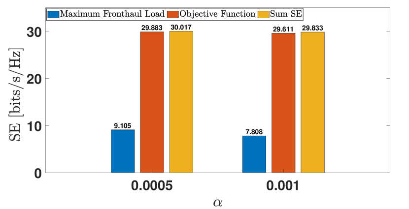
Figure 1: The variation of maximum fronthaul load on an AP, objective function, and the sum SE, when $M=50$.

Figure 1 shows the variations in maximum front-haul load, objective function, and the sum SE for two different regularization coefficient values, with the number of antennas fixed at $50$. This highlights how the penalty function affects the network’s maximum front-haul load and total sum-throughput. Notably, the objective function value consistently remains lower than the total SE value, exhibiting a drop attributed to the penalty function. When the regularization coefficient is increased by two times, the maximum front-haul load on an AP decreases by $14\%$. This reduction is due to the increased regularization coefficient, which limits AP-UE associations. As a consequence of the lesser number of AP-UE associations, there is a reduction in the sum SE by nearly $1\%$. Similarly, Figure 2 illustrates variability in maximum front-haul load, objective function, and sum SE for two different regularization coefficient values, however with $M$ set to 100. For this scenario too, when the regularization coefficient is increased two times, the maximum front-haul load and total SE show a similar decreasing trend as in Fig. 1. Therefore, the proposed approach effectively decreases the maximum front-haul load while not significantly reducing overall sum throughput, and this is achieved by a careful tuning of regularization coefficient.

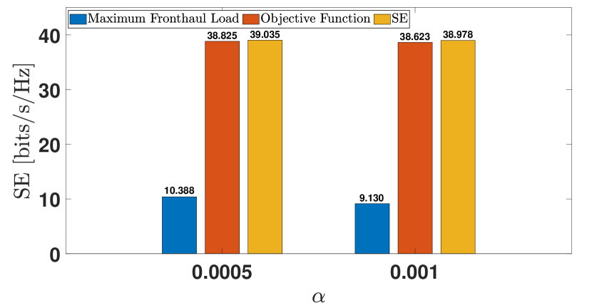
Figure 2: The variation of maximum front-haul load on an AP, objective function, and the sum SE, when $M=100$.

Examining Figures 1 and 2, we observe a noteworthy trend as the number of antennas ($M$) increases from 50 to 100. The maximum front-haul load increases by $14\%$ and $17\%$ with regularization coefficients ($\alpha$) of 0.0005 and 0.001, respectively. This growth can be attributed to the growing number of APs in the fixed area. As the AP count increases, there are more APs in the vicinity of each UE, resulting in a higher percentage of APs offering a strong channel or a larger large-scale fading coefficient for each UE. This gainful influence of numerous APs on the large-scale fading coefficient causes a change in the influence of the penalty function, allowing more APs to associate with each UE. While this increased association raises the maximum front-haul load, it also results in a significant ($30\%$) boost in the overall sum-throughput. In essence, the system responds to the increased AP count by increasing the strength of channels across numerous APs, hence increasing the network’s overall throughput. The penalty function is a dynamic component of this process, optimizing AP-UE associations to optimize the objective function while reducing negative affects via penalties.

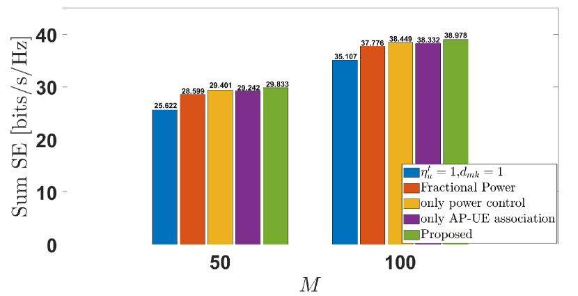
Figure 3: The variation of the sum SE for different scenarios, when $\alpha=0.001$.

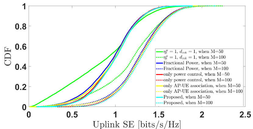
Figure 4: CDF vs per-UE SE for different scenarios, when $\alpha=0.001$.

Figures 3 and 4 illustrate the variation of sum SE and per-UE SE respectively, of the proposed solution in comparison to the following four scenarios: a) where UEs transmit at full power and are served by all APs; b) fractional power control [8]; c) where only power control is performed using the proposed algorithm; and d) where only AP-UE association is performed using the proposed algorithm.

Figure 3 shows that when AP-UE association and power control are carried out simultaneously, the achievable sum SE is the largest. The proposed solution’s sum SE surpasses that of scenarios ’a’, ’b’,’c’ and ’d’ by $16.5\%$, $4.3\%$, $1.5\%$ and $2\%$, respectively, when $M=50$. Additionally, for case with $M=100$, the proposed solution outperforms these scenarios by $11\%$, $3\%$, $1.3\%$, and $1.6\%$, respectively. This demonstrates the effectiveness of the proposed technique in optimizing the sum SE by jointly addressing the AP-UE association and power control problems. Notably, when only AP-UE association or only power control is conducted with the proposed method, the sum SE sees a improvement when compared to the other two scenarios ’a’ and ’b’. This improvement occurs while preserving the minimum QoS limitation. The proposed approach’s versatility and effectiveness are demonstrated by its ability to improve network performance even when improving just a single aspect of the system, like AP-UE association or power control.

Indeed, our proposed technique aims to enhance the sum SE. Figure 4 shows how our strategy has a significant influence on the $90\%-likely$ per-user SE. Our proposed scheme outperforms scenarios ’a’, ’b’, ’c’, and ’d’ in terms of $90\%-likely$ per-user SE by $175\%$, $22\%$, $4.7\%$, and $11.7\%$, respectively, at $M=50$. Similarly, for $M=100$, our approach outperforms the same cases by $52.3\%$, $6.7\%$, $2.1\%$, and $3.2\%$ in terms of $90\%-likely$ per-user SE. The findings illustrate an additional benefit of the method we propose, demonstrating its massive contribution to improve per-user throughput while also increasing the total throughput.

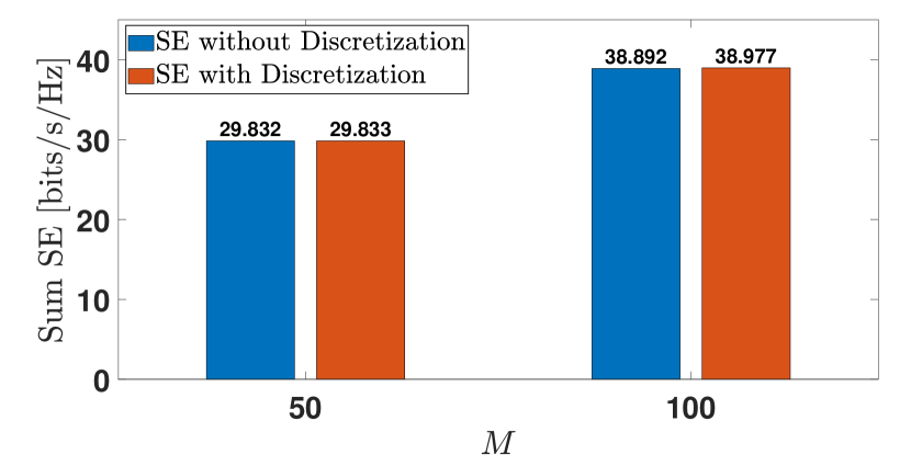
Figure 5: The variation of SE with and without discretization of elements of D.

In Figure 5, we provide a numerical justification for relaxation proposed in (5). It shows the variation of the SE with and without the discretization of matrix D. The figure shows that for $m=50$, the variation in the SE is negligible with and without the discretization of elements of matrix D. For the case when $m=100$, the difference in SE is mere $0.2\%$. The negligible SE variation can be attributed to the fact that penalty parameter does not force elements of matrix D too much away from zero or one, thus our proposed solution does not require additional algorithm for AP-UE association.

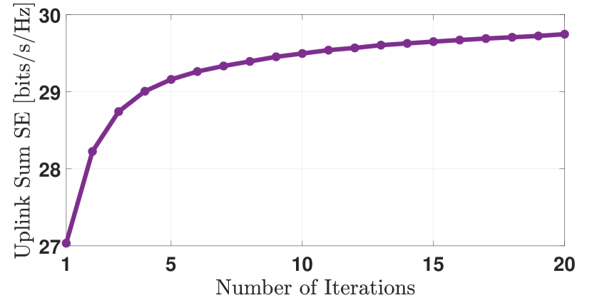
Figure 6: The convergence graph of Algorithm 1, when $\alpha=0.001$, $T=30$ and $M=50$.

In Figure 6, we provide a numerical evidence for the convergence Algorithm 1. The figure shows that as the number of iterations increases, so does the value of the objective function, leading up in a non-decreasing function. However, the rate of rise gradually decreases, ensuring that the rate of increase of objective function finally becomes lower than the defined tolerance of $\epsilon=5\times 10^{-3}$. This observation guarantees the convergence of Algorithm 1.

V Conclusion

In this work, we address the challenge of joint AP-UE association and power control in uplink distributed mMIMO systems by introducing an l1-penalty based joint mixed-integer non-convex optimization problem. Our technique strives to maximize system throughput while adhering to minimum quality of service (QoS) requirements. For tackling this optimization problem, we reformulate the original problem and develop an iterative technique that guarantees convergence. Through numerical simulations, we demonstrate that optimizing AP-UE association and power control factor jointly results in a significant increase in the system’s sum-throughput when compared to the cases where just one parameter is optimized. Another interesting observation is the significant decrease in the maximum front-haul load at the expense of marginal drop in the sum-throughput. A highlight of our proposed scheme is the significant enhancement in the $90\%-likely$ per-UE SE. It demonstrates the significance and efficacy of the proposed scheme when compared to other schemes in maximizing system performance and providing a better user experience in uplink distributed mMIMO systems. Overall, our findings underline the need of optimizing AP-UE association and power regulation simultaneously, emphasizing the potential for significant throughput gains and per-user SE improvements in uplink distributed mMIMO systems.

Convergence Analysis : For the convergence analysis of the Algorithm 1, the primary goal is to prove that both optimization problem defined in (13) and (14) converges to the their respective optimal solutions. Thereafter, we prove that in each iteration of Algorithm 1, the optimization function in (12a) is non-decreasing with respect to $\mathbf{\eta^{u}}$ and D.

The feasible set of smooth concave objective function $\mathbb{F}_{1}$ (13a), articulated by Equation (13b), is closed and convex. As a result, $\mathbb{F}_{1}$ is inherently continuous and differentiable over its feasible set, implying the existence of an optimal solution for $\mathbb{F}_{1}$. The feasible set, defined by Equation (14b), of non-smooth concave objective function $\mathbb{F}_{2}$ (14a), is closed and convex. However, $\mathbb{F}_{2}$ due to the l1-penalty lacks continuous differentiability over its feasible set. Despite this, $\mathbb{F}_{2}$ can be separated into smooth and non-smooth part. The convergence of $\mathbb{F}_{2}$ is guaranteed if gradient of the smooth part of $\mathbb{F}_{2}$ is Lipschitz continuous over its feasible set [18]. Thus the second derivative of the $\mathbb{F}_{2}$ without the non-smooth part with respect to the AP-UE association variable, $d_{mt}$ is given by :

$$\frac{\partial^{2}\mathbb{F}_{1}}{\partial d_{mt}^{2}}=\sum\limits_{t=1}^{T}\left(2w^{\prime}(1+\mathbf{\Gamma})A^{2}p_{u}\eta_{t}^{u}\gamma^{2}_{mt}-\frac{P(\sum\limits_{t^{\prime}=1}^{T}A^{2}p_{u}\eta_{t^{\prime}}^{u}\left|\Psi^{H}_{t}\Psi_{t^{\prime}}\right|^{2}(\gamma_{mt}\frac{\beta_{mt^{\prime}}}{\beta_{mt}})^{2})}{Q}-\frac{PQ^{\prime}}{Q}+\frac{PQ^{\prime 2}}{Q^{2}}\right),$$ (15)

where $P$, $Q$ and $Q^{\prime}$ are given by, respectively:

$$P=w^{\prime}(1+\mathbf{\Gamma})A^{2}p_{u}\eta_{t}^{u}(\sum\limits_{m\in\mathcal{M}}d_{mt}\gamma_{mt})^{2},$$ (16)

$$Q=\sum\limits_{t^{\prime}=1}^{T}A^{2}p_{u}\eta_{t^{\prime}}^{u}\left|\Psi^{H}_{t}\Psi_{t^{\prime}}\right|^{2}(\sum\limits_{m\in\mathcal{M}}d_{mt}\gamma_{mt}\frac{\beta_{mt^{\prime}}}{\beta_{mt}})^{2}+\sum\limits_{t^{\prime}=1}^{T}Ap_{u}\eta_{t^{\prime}}^{u}\sum\limits_{m\in\mathcal{M}}d_{mt}\gamma_{mt}\beta_{mt^{\prime}}+\sum\limits_{m\in\mathcal{M}}Ad_{mt}\gamma_{mt},$$ (17)

$$Q^{\prime}=\sum\limits_{t^{\prime}=1}^{T}A^{2}p_{u}\eta_{t^{\prime}}^{u}\left|\Psi^{H}_{t}\Psi_{t^{\prime}}\right|^{2}(\sum\limits_{m\in\mathcal{M}}d_{mt}\gamma_{mt}\frac{\beta_{mt^{\prime}}}{\beta_{mt}})\gamma_{mt}\frac{\beta_{mt^{\prime}}}{\beta_{mt}}+\sum\limits_{t^{\prime}=1}^{T}Ap_{u}\eta_{t^{\prime}}^{u}\gamma_{mt}\beta_{mt^{\prime}}+A\gamma_{mt}$$ (18)

Notably, all the terms in the above double partial derivative (15) are bounded from above, thus the gradient of the $\mathbb{F}_{2}$ is Lipschitz continuous over its feasible set.

To prove the non-decreasing nature of the optimization function $f(\mathbf{\eta^{u}},\textbf{D})$ defined in (12a), let ${\mathbf{\eta^{u}}}^{*}$ be the optimal value of function $f$, when D is fixed. Then, for fixed D, the inequality $f({\mathbf{\eta^{u}}}^{*},{\textbf{D}}^{(i)})\geq f({\mathbf{\eta^{u}}}^{(i)},{\textbf{D}}^{(i)})$ always holds due to the concavity of the function $f$. For the optimal $\textbf{D}^{*}$, when $\mathbf{\eta^{u}}$ is fixed at ${\mathbf{\eta^{u}}}^{(i+1)}$, the inequality $f({\mathbf{\eta^{u}}}^{(i+1)},{\textbf{D}}^{*})\geq f({\mathbf{\eta^{u}}}^{(i+1)},{\textbf{D}}^{(i)})$ always holds as $f$ is concave for fixed D. It can be inferred that $f({\mathbf{\eta^{u}}}^{(i+1)},{\textbf{D}}^{(i+1)})\geq f({\mathbf{\eta^{u}}}^{(i)},{\textbf{D}}^{(i)})$, indicating $f$ is non-decreasing in each iteration. It makes the optimization function monotonically increasing in each iteration and also the optimization function is bounded from above, thereby guaranteeing the convergence of the proposed algorithm.

References

- [1] E. G. Larsson, O. Edfors, F. Tufvesson, and T. L. Marzetta, “Massive MIMO for next generation wireless systems,” IEEE Commun. Magazine, vol. 52, no. 2, pp. 186–195, 2014.
- [2] E. Björnson, J. Hoydis, L. Sanguinetti et al., “Massive MIMO networks: Spectral, energy, and hardware efficiency,” Foundations and Trends® in Signal Processing, vol. 11, no. 3-4, pp. 154–655, 2017.
- [3] H. Q. Ngo, A. Ashikhmin, H. Yang, E. G. Larsson, and T. L. Marzetta, “Cell-free massive MIMO versus small cells,” IEEE Trans. on Wireless Commun., vol. 16, no. 3, pp. 1834–1850, 2017.
- [4] E. Nayebi, A. Ashikhmin, T. L. Marzetta, H. Yang, and B. D. Rao, “Precoding and power optimization in cell-free massive MIMO systems,” IEEE Trans on Wireless Commun, vol. 16, no. 7, pp. 4445–4459, 2017.
- [5] H. Q. Ngo, L.-N. Tran, T. Q. Duong, M. Matthaiou, and E. G. Larsson, “On the total energy efficiency of cell-free massive MIMO,” IEEE Trans. on Green Commun. and Network., vol. 2, no. 1, pp. 25–39, 2017.
- [6] E. Björnson and L. Sanguinetti, “Scalable cell-free massive MIMO systems,” IEEE Trans. on Commun., vol. 68, no. 7, pp. 4247–4261, 2020.
- [7] S. Buzzi and C. D’Andrea, “Cell-free massive mimo: User-centric approach,” IEEE Wireless Commun. Letters, vol. 6, no. 6, pp. 706–709, 2017.
- [8] R. Nikbakht, R. Mosayebi, and A. Lozano, “Uplink fractional power control and downlink power allocation for cell-free networks,” IEEE Wireless Commun. Letters, vol. 9, no. 6, pp. 774–777, 2020.
- [9] S. Buzzi, C. D’Andrea, A. Zappone, and C. D’Elia, “User-centric 5g cellular networks: Resource allocation and comparison with the cell-free massive mimo approach,” IEEE Trans. on Wireless Commun., vol. 19, no. 2, pp. 1250–1264, 2019.
- [10] N. Ghiasi, S. Mashhadi, S. Farahmand, S. M. Razavizadeh, and I. Lee, “Energy efficient ap selection for cell-free massive mimo systems: Deep reinforcement learning approach,” IEEE Trans. on Green Commun. and Network., vol. 7, no. 1, pp. 29–41, 2022.
- [11] T. X. Vu, S. Chatzinotas, S. ShahbazPanahi, and B. Ottersten, “Joint power allocation and access point selection for cell-free massive mimo,” in Proc. IEEE ICC, Online, June 2020.
- [12] M. Guenach, A. A. Gorji, and A. Bourdoux, “A deep neural architecture for real-time access point scheduling in uplink cell-free massive mimo,” IEEE Trans. on Wireless Commun., vol. 21, no. 3, pp. 1529–1541, 2021.
- [13] H. Q. Ngo, H. Tataria, M. Matthaiou, S. Jin, and E. G. Larsson, “On the performance of cell-free massive mimo in ricean fading,” in Proc. ACSSC, USA, Oct. 2018.
- [14] M. Guenach, A. A. Gorji, and A. Bourdoux, “Joint power control and access point scheduling in fronthaul-constrained uplink cell-free massive mimo systems,” IEEE Trans. on Commun., vol. 69, no. 4, pp. 2709–2722, 2020.
- [15] Y. Tsuruoka, J. Tsujii, and S. Ananiadou, “Stochastic gradient descent training for l1-regularized log-linear models with cumulative penalty,” in Proc. of the Joint Conference ACL and IJCNLP, Singapore, Aug. 2009.
- [16] T. C. Mai, H. Q. Ngo, M. Egan, and T. Q. Duong, “Pilot power control for cell-free massive mimo,” IEEE Trans. on Veh. Techno., vol. 67, no. 11, pp. 11 264–11 268, 2018.
- [17] K. Shen and W. Yu, “Fractional programming for communication systems—part ii: Uplink scheduling via matching,” IEEE Trans. on Signal Processing, vol. 66, no. 10, pp. 2631–2644, 2018.
- [18] G. Scutari, F. Facchinei, and L. Lampariello, “Parallel and distributed methods for constrained nonconvex optimization—part i: Theory,” IEEE Trans. on Signal Processing, vol. 65, no. 8, pp. 1929–1944, 2016.