Embeddings and near-neighbor searching with constant additive error for hyperbolic spaces

Abstract

We give an embedding of the Poincaré halfspace $\mathbb{H}^{D}$ into a discrete metric space based on a binary tiling of $\mathbb{H}^{D}$, with additive distortion $O(\log D)$. It yields the following results. We show that any subset $P$ of $n$ points in $\mathbb{H}^{D}$ can be embedded into a graph-metric with $2^{O(D)}n$ vertices and edges, and with additive distortion $O(\log D)$. We also show how to construct, for any $k$, an $O(k\log D)$-purely additive spanner of $P$ with $2^{O(D)}n$ Steiner vertices and $2^{O(D)}n\cdot\lambda_{k}(n)$ edges, where $\lambda_{k}(n)$ is the $k$th-row inverse Ackermann function. Finally, we present a data structure for approximate near-neighbor searching in $\mathbb{H}^{D}$, with construction time $2^{O(D)}n\log n$, query time $2^{O(D)}\log n$ and additive error $O(\log D)$. These constructions can be done in $2^{O(D)}n\log n$ time.

1 Introduction

The Poincaré halfplane $\mathbb{H}^{2}$ is perhaps the most common model of hyperbolic spaces, together with the Poincaré disk which it is isometric to. The points of $\mathbb{H}^{2}$ are the points $(x,z)$, $z>0$ of the upper halfplane of $\mathbb{R}^{2}$. The shortest paths in $\mathbb{H}^{2}$, called geodesics, are arcs of circles orthogonal to the $x$-axis (Figure 1a) and the arc length is given by integrating the relation $ds^{2}=(dx^{2}+dz^{2})/z^{2}$. More generally, the Poincaré halfspace is a $D$-dimensional model of hyperbolic space, that consists of points $(x,z)$ where $x\in\mathbb{R}^{D-1}$ and $z$ is a positive real number. In $\mathbb{H}^{D}$, the expression of $ds^{2}$ is the same, but $x$ is now a point in $\mathbb{R}^{D-1}$, and geodesics are arcs of circles orthogonal to the hyperplane $z=0$.

Hyperbolic spaces behave very differently from Euclidean spaces in some respects. For instance, in fixed dimension, the volume of a hyperbolic ball grows exponentially with its radius, while the radius of a Euclidean ball grows polynomially. A triangle, formed by connecting three points by the geodesic between each pair of these points, is thin in the sense that from any point on an edge, there is a point on another edge at distance bounded by a constant.

As a consequence, hyperbolic spaces are sometimes more suitable than Euclidean spaces to represent some types of data. It has been shown, for instance, that there are better embeddings of the internet graph into hyperbolic spaces, compared with its embeddings into Euclidean spaces [12]. There has also been recent interest in hyperbolic spaces in the context of artificial neural networks [5].

In this paper, we present embeddings of finite subsets of $\mathbb{H}^{D}$ into graph metrics with a linear number of edges, and a constant additive distortion, when $D=O(1)$. As an application, we present an approximate near-neighbor data structure with constant additive distortion. These two results have no multiplicative distortion.

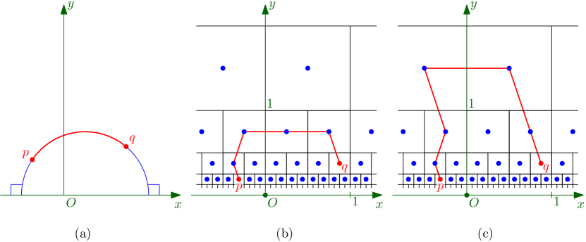
Figure 1: Three models of hyperbolic spaces. (a) The Poincaré halfplane $\mathbb{H}^{2}$. (b) The first discrete model $(\mathbb{B}^{2},d_{1})$, with a shortest path of length $d_{1}(p,q)=5$. (c) The second discrete model $(\mathbb{B}^{2},d_{2})$, with a shortest path of length $d_{2}(p,q)=6$.

1.1 Our results.

Given two metric spaces $(M,d)$ and $(M^{\prime},d^{\prime})$, we say that a mapping $\varphi:M\to M^{\prime}$ is an embedding with additive distortion $\Delta$ if for any two points $p,q\in M$, we have

$$d(p,q)-\Delta\leqslant d^{\prime}(\varphi(p),\varphi(q))\leqslant d(p,q)+\Delta.$$

Our first result (Theorem 14) is an embedding of $\mathbb{H}^{D}$ with additive distortion $O(\log D)$ into a discrete metric space $(\mathbb{B}^{D},d_{1})$ that is obtained from a binary tiling of $\mathbb{H}^{D}$. (See Section 2 and Figure 1b.)

Given a subset $P$ of $n$ points of a metric space $(M,d)$, a purely-additive spanner of $P$ with distortion $\Delta$ and $n^{\prime}$ Steiner points is a graph $G(V,E)$ where $V=P\cup S$, the points in $S$ are called Steiner points, $|S|=n^{\prime}$, the length of any edge $pq$ is $d(p,q)$, and the shortest path distance $d_{G}(\cdot)$ in this graph satisfies

$$d(p,q)\leqslant d_{G}(p,q)\leqslant d(p,q)+\Delta\quad\text{for all }p,q\in P.$$

We show, for any subset $P$ of $n$ points of $(\mathbb{B}^{D},d_{1})$, how to construct in $2^{O(D)}n\log n$ a purely-additive spanner of $P$ with $2^{O(n)}$ edges and Steiner vertices, and distortion $2$. (Theorem 16.)

Based on the two results above, we first obtain an embedding of any subset $P$ of $n$ points of $\mathbb{H}^{D}$ into a graph metric with $2^{O(D)}n$ vertices and edges, and additive distortion $O(k\log D)$. We also obtain an $O(k\log D)$ purely additive spanner of $P$ with $2^{O(D)}n$ vertices and $2^{O(D)}n\cdot\lambda_{k}(n)$ Steiner vertices and edges, where $\lambda_{k}(n)$ is the $k$th-row inverse Ackermann function.

Given a subset $P$ of $n$ points of a metric space $(M,d)$, and a query point $q\in P$, the nearest neighbor of $q$ is the point $p\in P$ such that $d(p,q)$ is minimum. An approximate nearest neighbor (ANN) with additive distortion $\Delta$ is a point $p^{\prime}\in P$ such that $d(p^{\prime},q)\leqslant d(p,q)+\Delta$.

We give data structures for answering ANN queries in $(\mathbb{B}^{D},d_{1})$ and in $\mathbb{H}^{D}$ with query time $2^{O(D)}\log n$ and construction time $2^{O(D)}n\log n$. For $(\mathbb{B}^{D},d_{1})$, the additive distortion is 2, and for $\mathbb{H}^{D}$, it is $O(\log D)$. (See Corollary 20 and 21.) These data structures are obtained by augmenting our spanner structures, and performing queries in the corresponding compressed quadtrees.

1.2 Comparison with previous work.

Spanners have been studied in the more general context of an arbitrary weighted graph metric [1]. For instance, one can find a $t$-multiplicative spanner of total weight $(1+1/t)$ times the weight of a minimum spanning tree.

For Euclidean metrics, it was shown that there are spanners with a linear number of edges, and multiplicative distortion arbitrarily close to 1 [2]. One difference with this paper is that we consider an additive distortion. In the worst case, one cannot hope to find a non-trivial additive spanner for the Euclidean metric, because the additive error for a given graph can be made arbitrarily larger by simply scaling up all the distances.

Gromov-hyperbolicity is a notion of hyperbolicity that applies to any metric space $(M,d)$, including discrete metric spaces. These spaces have the property that for any 4 points $p,q,r,s\in M$, the largest two sums of distances among $d(p,q)+d(r,s)$, $d(p,r)+d(q,s)$, $d(p,s)+d(q,r)$ differ by a constant. As shown by Gromov [6], any metric space of $n$ points with hyperbolicity $\delta$ can be embedded into a tree-metric with additive distortion $O(\delta\log n)$. The Poincaré half-space has hyperbolicity $O(1)$, so this result applies to a more general type of hyperbolic spaces than our embedding of $\mathbb{H}^{D}$ into a graph metric with $O(n)$ edges. On the other hand, we obtain an additive distortion $O(1)$ in constant dimension, while Gromov’s construction gives $O(\log n)$ in our case. Chepoi et al. [4] give additive $O(\delta\log n)$ spanners with $O(\delta n)$ edges for unit graph metrics (i.e. metrics for graphs where each edge weight is equal to 1) that are $\delta$-hyperbolic. Compared with our result, it allows arbitrary hyperbolicity, but it is restricted to unit graphs, and the distortion is logarithmic.

There has also been some work on problems other than spanners and embeddings in hyperbolic spaces. Lee and Krautghamer [10] presented results on several proximity problems in Gromov-hyperbolic spaces. Kisfaludi-Bak et al. gave an algorithm for the TSP problem in $\mathbb{H}^{2}$ and presented a quadtree-like data structure for proximity problems in $\mathbb{H}^{D}$ [8, 9].

More recently, Kisfaludi-Bak and van Wordragen [9] gave an ANN data structure and Steiner spanners for $\mathbb{H}^{D}$ with multiplicative error $(1+\varepsilon)$. Their approach is based on the same binary tiling that we use, but they derive from it a non-trivial type of quadtree that is taylored for providing multiplicative guarantees in hyperbolic spaces. The lower bound that they present on spanners without Steiner points imply that in order to achieve additive error, Steiner points are also required.

1.3 Our approach.

We use an approximation of the Poincaré halfspace $(\mathbb{H}^{D},d_{H})$ by a discrete metric space $(\mathbb{B}^{D},d_{1})$ where the points are centers of hypercubes (called cells) whose sizes grow exponentially with $y$. (See Figure 1b.) The distance between two points $p,q$ is the minimum number of cells that are crossed when going from $p$ to $q$. This discrete model was mentioned, for instance, by Cannon et al. [3]. We present these models of hyperbolic spaces in Section 2.

We introduce a different distance function $d_{2}$ over $\mathbb{B}^{D}$: we go upwards from $p$ and $q$ until we reach adjacent squares, and then we connect the subpaths using a single horizontal edge. (See Figure 1c.). This model is not a metric as it does not satisfy the triangle inequality. In Section 3, we show that $d_{1}$ and $d_{2}$ differ by at most 2. Then in Section 6, we show that the overlay of the shortest paths according to $d_{2}$ has linear complexity, and hence gives a 2-additive spanner of linear size with respect to $d_{1}$. (See Figure 7.)

In Section 4, we show that over $\mathbb{B}^{D}$, the distance functions $d_{H}$, $d_{1}$, $d_{2}$ are within a constant additive term from each other. This allows us, in Section 7, to use the spanner we constructed in the discrete model to obtain an embedding into a graph metric with $O(\log D)$-additive distortion. Then using a transitive-closure spanner, we turn it into a spanner with respect to $d_{H}$ embedded in $\mathbb{H}^{D}$.

The efficient constructions of our embeddings, spanners and ANN-data structure, as well as the bound on their size, are based on compressed quadtrees. Our discrete models lend themselves well to the use of quadtrees.

2 Models of hyperbolic spaces

Figure 1 shows the three models of hyperbolic spaces that we consider in this paper, when $D=2$. The Poincaré halfplane $(\mathbb{H}^{2},d_{H})$ is shown in Figure 1a. It is a model of 2-dimensional hyperbolic space with constant negative curvature $-1$. The halfplane $\mathbb{H}^{2}$ consists of the points $p=(x(p),z(p))$ where $z(p)>0$. The geodesics in $(\mathbb{H}^{2},d_{H})$ are arcs of semi-circles that are orthogonal to the $x$-axis. (See Figure 1a.)

More generally, when $D\geqslant 2$, the Poincaré halfspace $\mathbb{H}^{D}$ consists of the points $p=(x(p),z(p))$ where $x\in\mathbb{R}^{D-1}$ and $z$ is a positive real number. The distance $d_{H}(p,q)$ between two points $p$ and $q$ is the length of the geodesic from $p$ to $q$, where the arc-length is given by the relation $ds^{2}=(dx^{2}+dz^{2})/z^{2}$. This distance is given by the expression

$$d_{H}(p,q)=2\operatorname{arsinh}\left(\frac{1}{2}{\frac{\|pq\|}{\sqrt{z(p)z(q)}}}\right)$$

where $\|\cdot\|$ is the Euclidean norm. In the special case where $x(p)=x(q)$ and $z(q)>z(p)$, it is simply $d_{H}(p,q)=\ln(z(q)/z(p))$. The geodesics in $(\mathbb{H}^{D},d_{H})$ are arcs of semi-circles that are orthogonal to the hyperplane $z=0$.

The first discrete model $(\mathbb{B}^{D},d_{1})$ is defined using a binary tiling of $\mathbb{H}^{D}$ with the hypercubes, called cells,

$$\mathcal{C}=[k_{1}2^{i},(k_{1}+1)2^{i}]\times[k_{2}2^{i},(k_{2}+1)2^{i}]\times\dots\times[k_{D-1}2^{i},(k_{D-1}+1)2^{i}]\times[2^{i},2^{i+1}]$$

where $k_{1},k_{2},\dots,k_{D-1},i\in\mathbb{Z}$. (See Figure 1b for an example when $D=2$.) The level of this cell $\mathcal{C}$ is the integer $\mathrm{lev}(\mathcal{C})=i$, and its width is $2^{i}$.

The parent of a cell $\mathcal{C}$ at level $i$ is the cell at level $i+1$ whose bottom facet contains the upper facet of $\mathcal{C}$. The children of $\mathcal{C}$ are the cells whose parent is $\mathcal{C}$, hence $\mathcal{C}$ has $2^{D-1}$ children. An ancestor of $\mathcal{C}$ is either the parent of $\mathcal{C}$, or a parent of an ancestor of $\mathcal{C}$. A descendent of $\mathcal{C}$ is either a child of $\mathcal{C}$, or a descendent of a child of $\mathcal{C}$. The horizontal neighbors of $\mathcal{C}$ are the cells at level $i$ that intersect $\mathcal{C}$ along their boundary, hence $\mathcal{C}$ has $3^{D-1}-1$ horizontal neighbors.

We denote by $b(\mathcal{C})$ the center of the cell $\mathcal{C}$, so the $z$-coordinate of $b(\mathcal{C})$ is $z(b(\mathcal{C}))=3\cdot 2^{i-1}$ when $\mathrm{lev}(\mathcal{C})=i$. Then $\mathbb{B}^{D}$ is the set of the points $b(\mathcal{C})$ for all $\mathcal{C}$. The level $\mathrm{lev}(b(\mathcal{C}))$ of the point $b(\mathcal{C})$ is the level of $\mathcal{C}$. The parent, children, and horizontal neighbors of $\mathcal{C}$ are the point $b(\mathcal{C}^{\prime})$ where $\mathcal{C}^{\prime}$ is a parent, child or horizontal neighbor of $\mathcal{C}$, respectively.

From a point $p\in\mathbb{B}^{D}$, we allow the following types of moves:

• An upward move to the point whose cell is the parent of $\mathcal{C}(p)$.

• A downward move to a point whose cell is a child of $\mathcal{C}(p)$.

• A horizontal move to a point whose cell is a horizontal neighbor of $\mathcal{C}(p)$. (Hence, when moving horizontally, we allow to move along diagonals.)

(See Figure 2.)

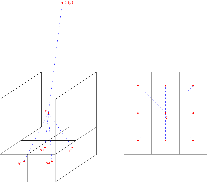
Figure 2: Possible moves in $\mathbb{B}^{3}$. (left) Vertical moves $U(p)$ and $D(p)\in\{q_{1},q_{2},q_{3},q_{4}\}$. (right) The 8 Horizontal moves $H(p)$, seen from above.

Then for any $p,q\in\mathbb{B}^{D}$, we define $d_{1}(p,q)$ to be the minimum number of moves that are needed to reach $q$ from $p$, and we define $d_{2}(p,q)$ to be the length of the shortest path from $p$ to $q$ that has at most one horizontal move. Figure 1(b) and (c) show examples of shortest paths in these models. A path from $p$ to $q$ consisting $d_{1}(p,q)$ such moves is called a $d_{1}$-path. Similarly, the path from $p$ to $q$ consisting of $d_{2}(p,q)$ moves, at most one of which being horizontal, is called a $d_{2}$-path. For any $p,q$, there is only one $d_{2}$-path from $p$ to $q$: If $p$ is neither a descendent or an ancestor of $q$, then this path bends at the lowest ancestors of $p$ and $q$ that are horizontally adjacent.

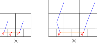
Figure 3: (a) A counterexample that shows that $d_{2}$ does not obey the triangle inequality: we have $d_{2}(p,q)=1$, $d_{2}(q,r)=1$ and $d_{2}(p,r)=3$ (b) An example where $d_{2}(p,q)=5=2+d_{1}(p,q)$.

The space $(\mathbb{B}^{D},d_{2})$ is not a metric space, but a semi-metric space, as it does not satisfy the triangle inequality. (See counterexample in Figure 3a).

3 Shortest paths in the discrete model

In this section, we study the structure, and give some bounds on the length of $d_{1}$-paths and $d_{2}$-paths.

Lemma 1.

Let $p,q\in\mathbb{B}^{D}$, and suppose that there is a $d_{1}$-path from $p$ to $q$ containing at least one upward move. Then there is a $d_{1}$- path from $p$ to $q$ whose first move is upward.

Proof.

Let $\rho=(p_{0},p_{1},\dots,p_{k})$ be a path of length $k=d_{1}(p_{0},p_{k})$ from $p=p_{0}$ to $q=p_{k}$, containing at least one upward move. If the first move of $\rho$ is upward, then we are done. Otherwise, Let $(p_{i},p_{i+1})$ be the first upward move, hence $(p_{i-1},p_{i})$ is horizontal or downward. If $(p_{i-1},p_{i})$ is downward, then we have $p_{i-1}=p_{i+1}$, so the path obtained from $\rho$ by deleting $p_{i}$ and $p_{i+1}$ is a path from $p$ to $q$ of length $d_{1}(p,q)-2$, a contradiction.

Now suppose that $(p_{i-1},p_{i})$ is horizontal. As $p_{i-1}$ and $p_{i}$ are horizontal neighbors, their parents either are equal, or are horizontal neighbors. So the parent of $p_{i-1}$ is either $p_{i+1}$, or is a horizontal neighbor of $p_{i+1}$. The parent of $p_{i-1}$ cannot be $p_{i+1}$, because if it were the case, we would obtain a path from $p$ to $q$ of length $d_{1}(p,q)-1$ by deleting $p_{i}$ from $\rho$. So the parent of $p_{i-1}$ is a horizontal neighbor $p^{\prime}_{i}$ of $p_{i+1}$. Hence, we obtain a path $\rho^{\prime}$ from $p$ to $q$ of length $d_{1}(p,q)$ by replacing $p_{i}$ with $p^{\prime}_{i}$.

The first upward move of $\rho^{\prime}$ is now $p_{i-1}p^{\prime}_{i}$, hence it has been moved one position to the left. By repeating this process $i-1$ times, we find a $d_{1}$-path from $p$ to $q$ that starts with an upward move. ∎

Lemma 2.

For any $p,q\in\mathbb{B}^{D}$, there is a $d_{1}$-path from $p$ to $q$ that consists of $m_{1}$ upward moves, followed by $m_{2}$ horizontal moves, and finally $m_{3}$ downward moves, where $m_{1},m_{2},m_{3}\in\mathbb{N}$.

Proof.

By applying Lemma 1 repeatedly, we obtain a $d_{1}$-path from $p$ to $q$ consisting of a sequence $\alpha$ of upward moves, followed by a sequence $\beta$ of horizontal or downward moves. Let $\gamma$ be the path obtained by following $\beta$ backward, hence $\gamma$ consists of upward or horizontal moves. We apply Lemma 1 to $\gamma$, until we obtain a path $\gamma$ consisting of upward moves followed by horizontal moves. Then the path obtained by following $\alpha$, and then following $\gamma$ backwards, has the desired property. ∎

Let $p,q\in\mathbb{B}^{D}$ be two points at the same level $i$. Their horizontal distance $\lambda(p,q)$ is the length of a shortest path from $p$ to $q$ consisting of horizontal moves only. It is given by the expression $\lambda(p,q)=\|x(p)x(q)\|_{\infty}/2^{i}$ where $\|\cdot\|_{\infty}$ is the $L^{\infty}$ norm.

Lemma 3.

If $p$ and $q$ are two points of $\mathbb{B}^{D}$ and $\mathrm{lev}(p)=\mathrm{lev}(q)$, then $2\lambda(p^{\prime},q^{\prime})-1\leqslant\lambda(p,q)\leqslant 2\lambda(p^{\prime},q^{\prime})+1$, where $p^{\prime}$ and $q^{\prime}$ are the parents of $p$ and $q$, respectively

Proof.

Let $\Delta_{i}=\{-2^{i-1},0,2^{i-1}\}^{D-1}$, then we have $\{x(p^{\prime})-x(p),x(q^{\prime})-x(q)\}\subset\Delta_{i}$. By the triangle inequality, it implies that $\|x(p^{\prime})x(q^{\prime})\|_{\infty}-2^{i}\leqslant\|x(p)x(q)\|_{\infty}\leqslant\|x(p^{\prime})x(q^{\prime})\|_{\infty}+2^{i}$. The result follows by dividing these inequalities by $2^{i}$. ∎

We now obtain a recurrence relation for $d_{1}(p,q)$ when $p$ and $q$ are at the same level.

Lemma 4.

If $p$ and $q$ are two points of $\mathbb{B}^{D}$ such that $\mathrm{lev}(p)=\mathrm{lev}(q)$, and if $\lambda=\lambda(p,q)$ is their horizontal distance, then

$$d_{1}(p,q)=\begin{cases}\lambda&\text{ if }\lambda\leqslant 4,\text{ and}\\ 2+d_{1}(p^{\prime},q^{\prime})&\text{ if }\lambda\geqslant 5.\end{cases}$$

where $p^{\prime}$ and $q^{\prime}$ are the respective parents of $p$ and $q$.

Proof.

By Lemma 2, there is a shortest path from $p$ to $q$ that consists of horizontal moves only (type 1), or that goes through $p^{\prime}$ and $q^{\prime}$ (type 2).

Any path of type 2 has length at least 3. So if $\lambda\leqslant 3$, there is a shortest path of type 1, and thus $d_{1}(p,q)=\lambda$.

If $\lambda=4$, then by Lemma 3, we have $\lambda(p^{\prime},q^{\prime})\geqslant 2$, so any path of type 2 has length more than 3. So there is a shortest path of type 1, and thus $d_{1}(p,q)=\lambda$.

Now suppose that $\lambda\geqslant 5$. Then by Lemma 3, we have $\lambda(p^{\prime},q^{\prime})\leqslant(1+\lambda)/2\leqslant\lambda-2$, and thus there is a shortest path which is of type 2. It follows that $d_{1}(p,q)=2+d_{1}(p^{\prime},q^{\prime})$. ∎

Lemma 5.

If $p$ and $q$ are two points of $\mathbb{B}^{D}$ and $\mathrm{lev}(p)=\mathrm{lev}(q)$, then $d_{2}(p,q)\leqslant d_{1}(p,q)+2$.

Proof.

Let $p^{\prime}$ and $q^{\prime}$ be the parents of $p$ and $q$, respectively. Let $p^{\prime\prime}$ and $q^{\prime\prime}$ be the parents of $p^{\prime}$ and $q^{\prime}$, respectively. Let $\lambda=\lambda(p,q)$, $\lambda^{\prime}=\lambda(p^{\prime},q^{\prime})$ and $\lambda^{\prime\prime}=\lambda(p^{\prime\prime},q^{\prime\prime}).$ We make a proof by induction on $\lambda$.

We first handle the basis cases.

• If $\lambda=0$, then $p=q$ and thus $d_{2}(p,q)=d_{1}(p,q)=0$.

• If $\lambda=1$, then $p$ and $q$ are horizontal neighbors, and thus $d_{2}(p,q)=d_{1}(p,q)=1$.

• If $\lambda=2$, then $\lambda^{\prime}=1$ by Lemma 3. It follows that $d_{2}(p,q)=3$ and $d_{1}(p,q)=2$.

• If $\lambda=3$, then $1\leqslant\lambda^{\prime}\leqslant 2$, and $\lambda^{\prime\prime}\leqslant 1$ by Lemma 3. It follows that $d_{1}(p,q)=3$ and $d_{2}(p,q)\leqslant 5$.

• If $\lambda=4$, then $\lambda^{\prime}=2$ and $\lambda^{\prime\prime}=1$. It follows that $d_{1}(p,q)=4$ and $d_{2}(p,q)=5$.

Now suppose that $\lambda\geqslant 5$. It follows from Lemma 3 that $3\leqslant\lambda^{\prime}\leqslant(1+\lambda)/2<\lambda$. So by induction hypothesis, we have $d_{2}(p^{\prime},q^{\prime})\leqslant d_{1}(p^{\prime},q^{\prime})+2$. As $\lambda\geqslant 2$, we have $d_{2}(p,q)=d_{2}(p^{\prime},q^{\prime})+2$, and thus $d_{2}(p,q)\leqslant d_{1}(p^{\prime},q^{\prime})+4$. By Lemma 4, we also have $d_{1}(p,q)=2+d_{1}(p^{\prime},q^{\prime})$. It follows that $d_{2}(p,q)\leqslant d_{1}(p,q)+2.$

∎

We can now prove the main result of this section.

Theorem 6.

For any two points $p,q\in\mathbb{B}^{2}$, we have $d_{1}(p,q)\leqslant d_{2}(p,q)\leqslant d_{1}(p,q)+2.$

Proof.

We have $d_{1}(p,q)\leqslant d_{2}(p,q)$ because $d_{1}(p,q)$ is the length of a shortest path from $p$ to $q$ in $\mathbb{B}^{D}$, and $d_{2}(p,q)$ is the length of some path from $p$ to $q$. We now prove the other side of the inequality.

If $p$ and $q$ are at the same level, then the result is given by Lemma 5. So we may assume that $p$ and $q$ are not at the same level. Without loss of generality, we assume that the $\mathrm{lev}(p)\leqslant\mathrm{lev}(q)$. Let $r$ be the ancestor of $p$ that is at the same level as $q$, and let $i=\mathrm{lev}(r)-\mathrm{lev}(p)$.

By definition, we have $d_{2}(p,q)=i+d_{2}(r,q)$. By Lemma 2, there is a shortest path from $p$ to $q$ going through $r$, and hence $d_{1}(p,q)=i+d_{1}(r,q)$. By Lemma 5, we have $d_{2}(r,q)\leqslant d_{1}(r,q)+2$. It follows that $d_{2}(p,q)\leqslant d_{1}(p,q)+2$. ∎

The bound in Theorem 6 is tight: In Figure 3b, we have $d_{2}(p,q)=d_{1}(p,q)+2=5$. Finally, we give a property of $d_{2}$-paths that will be needed later.

Let $p,q\in\mathbb{B}^{D}$ be such that $p$ is neither a parent nor a descendent of $q$, and $p\neq q$. Then the $d_{2}$-path $\rho$ from $p$ to $q$ contains exactly one horizontal move, from a point $\bar{p}$ to $\bar{q}$. We call the edge $\bar{p}\bar{q}$ the bridge of $\rho$. For instance, in Figure 3b, the bridge is the top edge of the blue path. The level of the bridge is $\mathrm{lev}(\bar{p})=\mathrm{lev}(\bar{q})$, which we denote $\mathrm{lev}(p,q)$.

When $p=q$, or $p$ is a descendent of $q$, we let $\mathrm{lev}(p,q)=\mathrm{lev}(q,p)=\mathrm{lev}(q)$. The lemma below allows us to approximate the level of a bridge.

Lemma 7.

Let $p$ and $q$ be two distinct points in $\mathbb{B}^{D}$ such that $p$ is neither a parent nor a descendent of $q$. Let $\ell=\lfloor\log_{2}\|x(p)x(q)\|_{\infty}\rfloor$. Then $\mathrm{lev}(p,q)-1\leqslant\ell\leqslant\mathrm{lev}(p,q)$.

Proof.

Without loss of generality, we assume that $\mathrm{lev}(p)\leqslant\mathrm{lev}(q)$. Let $i=\mathrm{lev}(p,q)$, and let $\bar{p}\bar{q}$ be the bridge of $d_{2}$-path from $p$ to $q$. As $\mathcal{C}(p)$ and $\mathcal{C}(q)$ are horizontal neighbors at level $i$, and $x(p)$ and $x(q)$ lie in the vertical projection of these cells onto the hyperplane $z=0$, we have $\|x(p)x(q)\|_{\infty}<2^{i+1}$, and thus $\ell\leqslant i$.

Suppose that $\mathrm{lev}(q)=i$. As $x(p)$ is not in the projection of $\mathcal{C}(q)$ onto the hyperplane $z=0$, we have $\|x(p)x(q)\|_{\infty}\geqslant 2^{i-1}$. It follows that $\ell\geqslant i-1$.

The remaining case is when $\mathrm{lev}(p)\leqslant\mathrm{lev}(q)\leqslant i-1$. Let $p^{\prime}$ be the first point after the bridge vertex $\bar{p}$ on the $d_{2}$-path from $\bar{p}$ to $p$, hence $p^{\prime}$ is a child of $\bar{p}$. We define $q^{\prime}$ in the same way. The points $x(p)$ and $x(q)$ are in the vertical projection of the cells $\mathcal{C}(p^{\prime})$ and $\mathcal{C}(q^{\prime})$ onto the hyperplane $z=0$. As $p^{\prime}$ and $q^{\prime}$ are at level $i-1$ and are not neighbors, it follows that $\|x(p)x(q)\|_{\infty}\geqslant 2^{i-1}$, and thus $\ell\geqslant i-1$. ∎

4 Embedding $\mathbb{H}^{D}$ into the discrete models

In this section, we give an embedding of the Poincaré half-space $\mathbb{H}^{D}$ into the discrete models $(\mathbb{B}^{D},d_{1})$ and $(\mathbb{B}^{D},d_{2})$ with additive distortion $O(\log D)$. Our embedding maps any point $p\in\mathbb{H}^{D}$ to the center $b(\mathcal{C})$ of the cell $\mathcal{C}$ of $\mathbb{H}^{D}$ that contains $p$. If several cells contain $p$, we take $b(p)$ to be center of a cell at the maximum level.

We first observe that for all $x\geqslant 1$,

$$\operatorname{arsinh}(x)=\ln(x+\sqrt{x^{2}+1})\leqslant\ln(x+\sqrt{2x^{2}})\leqslant\ln(x)+\ln(1+\sqrt{2})\leqslant\ln(x)+1.$$ (1)

We can then bound the hyperbolic distance between $p$ and $b(p)$.

Lemma 8.

For any $p\in\mathbb{H}^{D}$, we have $d_{H}(p,b(p))<\ln D$.

Proof.

Let $i=\mathrm{lev}(p)$. We have $\|pb(p)\|\leqslant 2^{i-1}\sqrt{D}$, $z(p)\geqslant 2^{i}$ and $z(b(p))\geqslant 2^{i}$. Therefore

$$d_{H}(p,b(p))=2\operatorname{arsinh}\left(\frac{1}{2}\frac{\|pb(p)\|}{\sqrt{z(p)z(b(p))}}\right)\leqslant 2\operatorname{arsinh}\left(\frac{1}{2}\frac{2^{i-1}\sqrt{D}}{2^{i}}\right)=2\operatorname{arsinh}\left(\frac{\sqrt{D}}{4}\right)$$

so by Inequality (1),

$$d_{H}(p,b(p))\leqslant 2\ln(\sqrt{D}/4)+2=\ln(D)+2-4\ln 2<\ln D.$$

∎

Let $p,q\in\mathbb{H}^{D}$ and let $h$ be the highest point on the geodesic from $p$ to $q$. Let $p^{\prime}$ and $q^{\prime}$ be the points vertically above $p$ and $q$, respectively, that are on the horizontal line through $h$. (See Figure 4a and  4b.)

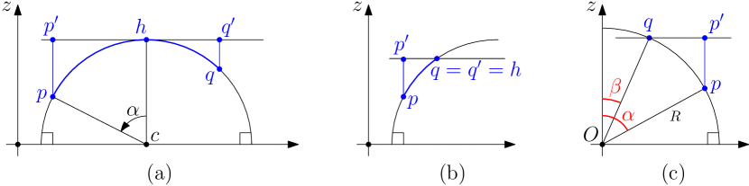
Figure 4: Lemma 9

Lemma 9.

For any $p,q\in\mathbb{H}^{D}$, we have $0\leqslant d_{H}(p,q)-d_{H}(p,p^{\prime})-d_{H}(q,q^{\prime})<2$.

Proof.

We first consider the special case where the geodesic from $p$ to $q$ is an arc of a circle of radius $R$ centered at the origin $O$, and the geodesic from $p$ to $q$ does not cross the $z$-axis. Let $\alpha$ and $\beta$ be the angles that $Op$ and $Oq$ make with the $z$-axis, respectively. Without loss of generality, we assume that $\alpha>\beta$. (See Figure 4c.)

By the triangle inequality, we have

$$d_{H}(p,q)-d_{H}(p,p^{\prime}) \leqslant d_{H}(p^{\prime},q)=2\operatorname{arsinh}\left(\frac{1}{2}\sqrt{\frac{R^{2}(\sin\alpha-\sin\beta)^{2}}{R^{2}\cos^{2}\beta}}\right)$$

$$\leqslant 2\operatorname{arsinh}\left(\frac{1}{2}\sqrt{\frac{(1-\sin\beta)^{2}}{\cos^{2}\beta}}\right)\leqslant 2\operatorname{arsinh}\left(\frac{1}{2}\sqrt{\frac{1-\sin^{2}\beta}{\cos^{2}\beta}}\right)$$

$$=2\operatorname{arsinh}(1/2)<1.$$

The inequality above applies whenever $q$ is the highest point on the geodesic arc $pq$, as in Figure 4b. When the geodesic arc $pq$ has a local maximum $h$ in its interior (See Figure 4a), we apply the inequality above twice through the point $h$ where $qq^{\prime}$ is tangent to the geodesic $pq$, which yields the result. (See Figure 4a.) ∎

Still using the same notation as in Figure 4, we have the following two observations.

Lemma 10.

Let $\hat{p}=b(p^{\prime})$ and $\hat{q}=b(q^{\prime})$. Then $d_{1}(\hat{p},\hat{q})\leqslant 5$.

Proof.

Let $R$ be the radius of the circle containing the geodesic arc $pq$. Suppose that $p^{\prime}q^{\prime}$ is tangent to this geodesic arc at $h$. (See Figure 4a.) Then $z(h)=R$, and the cells intersected by $p^{\prime}q^{\prime}$ are at a level $i$ such that $2^{i}\leqslant R<2^{i+1}$. So we have $i=\mathrm{lev}(\hat{p})=\mathrm{lev}(\hat{q})=\lfloor\log_{2}R\rfloor$. Since $\|p^{\prime}q^{\prime}\|\leqslant 2R$, we have $\|x(\hat{p})x(\hat{q})\|_{\infty}\leqslant 2R+2^{i}$, and since the width of the cells at level $i$ is at least $R/2$, the horizontal distance $\lambda(\hat{p},\hat{q})$ is at most $5$. It follows that $d_{1}(\hat{p},\hat{q})\leqslant 5$.

Now suppose that $h=q$ and the center of the circle containing the arc $pq$ is at the origin $O$. (See Figure 4c.) Let $\alpha$ and $\beta$ be the angles that $Op$ and $Oq$, respectively, make with the $z$-axis. Then the Euclidean length of $p^{\prime}q^{\prime}=p^{\prime}q$ is $R(\sin\alpha-\sin\beta)$ and the cells intersected by $p^{\prime}q^{\prime}$ have width at least $R\cos(\beta)/2$. Since

$$\frac{R(\sin\alpha-\sin\beta)}{R(\cos\beta)/2}\leqslant 2\frac{1-\sin\beta}{\cos\beta}\leqslant 2\frac{1-\sin^{2}\beta}{\cos^{2}\beta}=2,$$

by the same argument as above, $d_{1}(\hat{p},\hat{q})\leqslant 3$. ∎

The lemma below gives us a lower bound on the level of the bridge $\bar{p}\bar{q}$ when $p^{\prime}q^{\prime}$ is tangent to the geodesic arc $pq$, as in Figure 4a.

Lemma 11.

Suppose that $p$ and $q$ are two distinct points in $\mathbb{B}^{D}$ such that $p$ is neither a parent nor a descendent of $q$, and $h$ is between $p$ and $q$ along the geodesic arc $pq$. Then we have $\mathrm{lev}(p,q)\geqslant\log_{2}(z(h))-\log_{2}(D)/2-1$.

Proof.

The geodesic semi-circle through $p$ and $q$ has radius $z(h)$ and center $c=(x(h),0)$. Let $\alpha$ be the angle between the segment $cp$ and the segment $ch$. If $\alpha\leqslant\pi/3$, then $z(p)\geqslant z(h)/2$. Since $\mathrm{lev}(p,q)\geqslant\mathrm{lev}(p)$ and $z(p)=(3/2)2^{\mathrm{lev}(p)}$, it follows that

$$\mathrm{lev}(p,q)\geqslant\mathrm{lev}(p)=\log_{2}(z(p))-\log_{2}(3)+1\geqslant\log_{2}(z(h))-\log_{2}(3).$$

If $\alpha\geqslant\pi/3$, then $\|x(p)x(q)\|\geqslant\sqrt{3}z(h)/2$, so $\|x(p)x(q)\|_{\infty}\geqslant\sqrt{3}z(h)/(2\sqrt{D})$, and thus by Lemma 7, $\mathrm{lev}(p,q)\geqslant\log_{2}(\sqrt{3}z(h)/(2\sqrt{D}))\geqslant\log_{2}(z(h))-\log_{2}(D)/2-1$. ∎

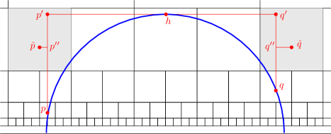
Figure 5: Proof of Lemma 13

We now prove that $d_{H}$, $d_{1}$ and $d_{2}$ differ by a $O(\log D)$ over $\mathbb{B}^{D}$. We begin with two special cases, and then we handle the general case.

Lemma 12.

For any $p,q\in\mathbb{B}^{D}$ such that $q$ is an ancestor of $p$, we have

$$\ln(2)\cdot d_{1}(p,q)\leqslant d_{H}(p,q)\leqslant\ln(2)\cdot d_{1}(p,q)+\ln(D)+O(1).$$

Proof.

Let $i=\mathrm{lev}(p)$ and $j=\mathrm{lev}(q)$. Let $r=(x(q),z(p))$. Then we have

$$d_{H}(p,q)\geqslant d_{H}(r,q)=\ln(z(q)/z(p))=\ln(2^{j-i})=(j-i)\ln 2.$$

and thus

$$d_{H}(p,q)\geqslant(j-i)\ln 2.$$ (2)

We now prove an upper bound on $d_{H}(p,q)$. Observe that $\|pq\|\leqslant 2^{j+1}\sqrt{D}$.

$$d_{H}(p,q)=2\operatorname{arsinh}\left(\frac{1}{2}\frac{\|pq\|}{\sqrt{z(p)z(q)}}\right)\leqslant 2\operatorname{arsinh}\left(\frac{2^{j+1}\sqrt{D}}{3\cdot 2^{(i+j)/2}}\right)\leqslant 2\operatorname{arsinh}\left({2^{(j-i+2)/2}\sqrt{D}}\right)$$

Then it follows from Inequality 1 that

$$d_{H}(p,q)\leqslant 2\ln\left(2^{(j-i+2)/2}\sqrt{D}\right)+1=\ln(2^{j-i+2})+\ln(D)+1=(j-i+2)\ln(2)+\ln(D)+1$$

and thus $d_{H}(p,q)\leqslant(j-i)\ln(2)+\ln(D)+\ln(4)+1$.

Together with (2), it shows that

$$(j-i)\ln 2\leqslant d_{H}(p,q)\leqslant(j-i)\ln(2)+\ln(D)+O(1)$$

. The result follows from $d_{1}(p,q)=j-i$. ∎

Lemma 13.

For any $p,q\in\mathbb{B}^{D}$, we have

$$-7\ln 2<d_{H}(p,q)-\ln(2)\cdot d_{1}(p,q)\leqslant\ln(D)+2+6\ln 2.$$

Proof.

Without loss of generality, we assume that $\mathrm{lev}(p)\leqslant\mathrm{lev}(q)$. The case where $q$ is an ancestor of $p$ is handled by Lemma 12, so we assume that $q$ is not an ancestor of $p$. Let $p^{\prime},q^{\prime}$ be defined as above. (See Figure 5.) Let $\hat{p}=b(p^{\prime})$, $\hat{q}=b(q^{\prime})$, $p^{\prime\prime}=(x(p),\hat{z}(p))$ and $q^{\prime\prime}=(x(q),\hat{z}(q))$. Let $i=\mathrm{lev}(p)$ and $j=\mathrm{lev}(\hat{p})=\mathrm{lev}(\hat{q})$.

By Lemma 10, we have $d_{1}(\hat{p},\hat{q})\leqslant 5$, and thus

$$d_{1}(p,q)\leqslant d_{1}(p,\hat{p})+d_{1}(q,\hat{q})+5.$$ (3)

Suppose that $q=\hat{q}$, and thus $d_{1}(q,\hat{q})=0$. Then the $d_{1}$-path from $p$ to $q$ goes through $\hat{p}$, and we have $d_{1}(p,q)\geqslant d_{1}(p,\hat{p})$, therefore $d_{1}(p,q)\geqslant d_{1}(p,\hat{p})+d_{1}(q,\hat{q})$.

Now suppose that $q\neq\hat{q}$. It implies that $p\neq\hat{p}$, and that $h$ is between $p$ and $q$ along the geodesic arc $pq$. So by Lemma 11, we have $\mathrm{lev}(p,q)\geqslant\log_{2}z(h)-\frac{1}{2}\log_{2}D-1$. As $z(h)\geqslant 2^{j}$, it implies that $\mathrm{lev}(p,q)\geqslant j-1-\frac{1}{2}\log_{2}D$. Hence the $d_{2}$-path $pq$ follows the path $p\hat{p}$ until $\hat{p}$, or a descendent of $\hat{p}$ at most $1+\frac{1}{2}\log_{2}D$ levels below $\hat{p}$. So the portion of the $d_{2}$-path $pq$ before the bridge has length at least $d_{1}(p,\hat{p})-\frac{1}{2}\log_{2}D-1$. Similarly, the portion after the bridge has length at least $d_{1}(q,\hat{q})-\frac{1}{2}\log_{2}D-1$. Therefore, $d_{2}(p,q)\geqslant d_{1}(p,\hat{p})+d_{1}(q,\hat{q})-2-\log_{2}D$. By Theorem 6, it implies that $d_{1}(p,q)\geqslant d_{1}(p,\hat{p})+d_{1}(q,\hat{q})-4-\log_{2}D$.

Together with Equation (3), it implies that, whether $q=\hat{q}$ or not,

$$-5\leqslant d_{1}(p,\hat{p})+d_{1}(q,\hat{q})-d_{1}(p,q)\leqslant 4+\log_{2}D.$$

We also have $d_{1}(p,\hat{p})=j-i$ and thus

$$d_{H}(p,p^{\prime\prime})=\ln(z(p^{\prime\prime})/z(p))=\ln\left(\left(3\cdot 2^{j-1}\right)/\left(3\cdot 2^{i-1}\right)\right)=(j-i)\ln 2=\ln(2)\cdot d_{1}(p,\hat{p}).$$

Similarly, we have $d_{H}(q,q^{\prime\prime})=\ln(2)\cdot d_{1}(q,\hat{q})$, and thus

$$-5\ln 2\leqslant d_{H}(p,p^{\prime\prime})+d_{H}(q,q^{\prime\prime})-\ln(2)\cdot d_{1}(p,q)\leqslant\ln(2)\cdot\log_{2}(D)+4\ln 2=\ln(D)+4\ln 2.$$

We also have $d_{H}(p^{\prime},p^{\prime\prime})=|\ln(z(p^{\prime})/z(p^{\prime\prime})|\leqslant\ln 2$ and, similarly, $d_{H}(q^{\prime},q^{\prime\prime})\leqslant\ln 2$. It follows that

$$-7\ln 2\leqslant d_{H}(p,p^{\prime})+d_{H}(q,q^{\prime})-\ln(2)\cdot d_{1}(p,q)\leqslant\ln(D)+6\ln 2.$$

The result follows from Lemma 9. ∎

It follows from Theorem 6, Lemma 8 and Lemma 13 that our embedding $b:\mathbb{H}^{D}\to\mathbb{B}^{D}$ gives $O(\log D)$ additive distortion with respect to $d_{1}$ and $d_{2}$.

Theorem 14.

For any $p,q\in\mathbb{H}^{D}$, we have $|d_{H}(p,q)-\ln(2)\cdot d_{1}(b(p),b(q))|\leqslant 3\ln(D)+O(1)$ and $|d_{H}(p,q)-\ln(2)\cdot d_{2}(b(p),b(q))|\leqslant 3\ln(D)+O(1)$.

5 Compressed quadtrees

In this section, we present compressed quadtrees [7], which will be needed for our graph metric embeddings and for approximate near neighbor searching. We will construct compressed quadtrees in $\mathbb{R}^{D-1}$.

The vertical projection of a point $p\in\mathbb{H}^{D}$ is $x(p)$, and the vertical projection $\mathcal{C}_{x}$ of a cell $\mathcal{C}$ of our binary tiling is the set of the vertical projections of the points in $\mathcal{C}$. So vertical projections of points and cells are in $\mathbb{R}^{D-1}$.

A quadtree cell is the vertical projection $\mathcal{C}_{x}$ of a cell $\mathcal{C}$ of our binary tiling of $\mathbb{H}^{D}$, such that $\mathcal{C}_{x}\subset[0,1]^{D-1}$. So a quadtree cell is of the form

$$[k_{1}2^{-i},(k_{1}+1)2^{-i}]\times\dots\times[k_{D-1}2^{-i},(k_{D-1}+1)2^{-i}]\text{ where }k_{1},\dots,k_{D-1}\in\mathbb{N}.$$

For any two cells $\mathcal{C}$ and $\mathcal{C}^{\prime}$ of our binary tiling such that $\mathcal{C}_{x},\mathcal{C}^{\prime}_{x}\subset[0,1]^{D-1}$, we say that $\mathcal{C}_{x}$ is a child (resp. parent, ancestor, descendent) of $\mathcal{C}^{\prime}_{x}$ if $\mathcal{C}$ is a child (resp. parent, ancestor, descendent) of $\mathcal{C}^{\prime}$. The level $\mathrm{lev}(\mathcal{C}_{x})$ of the quadtree cell $\mathcal{C}_{x}$ is $\mathrm{lev}(\mathcal{C})$, hence the level of a quadtree cell is non-positive.

Let $P^{\prime}$ be a set of $n$ points in $[0,1]^{D-1}$. A compressed quadtree $\mathcal{T}^{\prime}$ storing $P^{\prime}$ is a tree constructed as follows. Each node $\nu$ of $\mathcal{T}^{\prime}$ corresponds to a quadtree cell $\mathcal{C}_{x}(\nu)$. A quadtree cell that contains no point of $P^{\prime}$ is said to be empty, and it is a leaf cell if it contains at most one point of $P^{\prime}$. A leaf cell corresponds to a leaf node of $\mathcal{T}^{\prime}$. The root node corresponds to the cell $[0,1]^{D-1}$. The children of a node $\nu$ that is not a leaf are constructed as follows:

• If two or more children cells of $\mathcal{C}_{x}(\nu)$ are non-empty, then create a node $\nu_{i}$ corresponding to each such child cell, and make $\nu_{i}$ a child of $\nu$. In this case, $\nu$ is an ordinary node. (See Figure 6a.)

• If only one child of $\mathcal{C}_{x}(\nu)$ is non-empty, let $\nu^{\prime}$ be the descendent of $\nu$ such that $\mathcal{C}_{x}(\nu^{\prime})\cap P^{\prime}=\mathcal{C}_{x}(\nu)\cap P^{\prime}$ and the level of $\nu^{\prime}$ is minimum. Then $\nu^{\prime}$ is the only child of $\nu$, and $\nu$ is a compressed node. The region associated with $\nu$ is $\mathrm{rg}(\nu)=\mathcal{C}_{x}(\nu)-\mathcal{C}_{x}(\nu^{\prime})$. (See Figure 6b.)

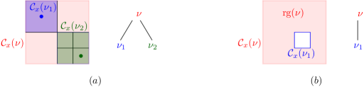
Figure 6: (a) An ordinary node $\nu$, with two children cells $\nu_{1}$ and $\nu_{2}$. (b) A compressed node $\nu$, with its child $\nu_{1}$. The region $\mathrm{rg}(\nu)$ is shaded in red.

The leaf cells and the regions of the compressed nodes form a partition of $\mathbb{R}^{D-1}$. This compressed quadtree $\mathcal{T}^{\prime}$ has $O(n)$ nodes, it can be constructed in $O(Dn\log n)$ time, and the node corresponding to the leaf cell or region containing a query point $q\in\mathbb{R}^{D-1}$ can be found in time $O(D\log n)$ time [7].

In addition, we can answer cell queries in $O(D\log n)$ time: Given a query quadtree cell $\mathcal{C}_{x}$, we can find the largest cell $\mathcal{C}_{x}^{-}$ stored in $\mathcal{T}^{\prime}$ such that $\mathcal{C}_{x}^{-}\subset\mathcal{C}_{x}$, and we can find the smallest cell $\mathcal{C}_{x}^{+}$ that contains $\mathcal{C}_{x}$.

6 Spanner in the discrete model

In this section, we give a 2-additive spanner $S$ in the first discrete model $(\mathbb{B}^{D},d_{1})$, for a set $P\subset\mathbb{B}^{D}$ of $n$ points. Our approach is the following: We overlay the $d_{2}$-paths of all pairs of points in $P$, and add a new vertex, called a Steiner vertex, at each point where such a path bends—in other words, we add a Steiner vertex at each endpoint of each bridge, if this endpoint is not in $P$. (See Figure 7.) We also add a Steiner vertex whenever two such $d_{2}$-paths merge. The length of an edge is the number of cell boundaries that it crosses.

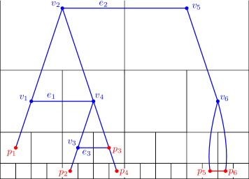
Figure 7: Our construction of a 2-additive spanner $S$ for the points $p_{1},\dots,p_{6}$ with respect to the metric $d_{1}$. The Steiner vertices are $v_{1},\dots,v_{6}$. The vertices $v_{1}$ and $v_{4}$ are the bending points of the $d_{2}$-path from $p_{1}$ to $p_{2}$, hence $v_{1}v_{4}$ is the bridge between $p_{1}$ and $p_{2}$. The vertex $v_{3}$ is the bending point of the $d_{2}$-path from $p_{2}$ to $p_{3}$. The distance from $p_{3}$ to $p_{6}$ within $S$ is $d_{S}(p_{3},p_{6})=6$, as the edge $v_{6}p_{6}$ has length 2. On the other hand, we have $d_{1}(p_{3},p_{5})=4$. The vertex $v_{6}$ is the Steiner vertex at which the $d_{2}$-paths from $p_{5}$ and $p_{6}$ to $p_{3}$ merge.

The resulting graph contains, by construction, a path of length $d_{2}(p,q)$ between any two points $p,q\in P$. By Theorem 6, it follows that $S$ contains a path of length at most $d_{1}(p,q)+2$ for any $p,q\in P$.

Proposition 15.

The graph $S$ described above is a 2-additive spanner of $P$ with respect to the discrete metric $d_{1}$. More precisely, for any $p,q\in\mathbb{H}^{D}$, there is a path in $S$ from $p$ to $q$ of length at least $d_{1}(p,q)$ and at most $d_{1}(p,q)+2$.

Using compressed quadtrees (Section 5), we now give a bound on the size of $S$, as well its construction time.

Let $P$ be our input set of points in $\mathbb{H}^{D}$, and let $x(P)=\{x(p):p\in P\}$ be its vertical projection. Without loss of generality, we assume that $x(P)\subset[0,1]^{D-1}$. If it were not the case, we could apply to $P$ a scaling transformation centered at $O$ followed by a horizontal translation so that the vertical projection of $P$ is in $[0,1]^{D-1}$, and since $d_{H}(\cdot)$ is invariant under these transformations, we do not change the problem.

We now construct a compressed quadtree $\mathcal{T}$ for $x(P)$, but with the following change. Let $p\in P$, then there is a cell $\mathcal{C}(p)$ of $\mathbb{B}^{D}$ such that $p$ is the center of $\mathcal{C}(p)$. Then we store $p$ at the node $\nu$ of $\mathcal{T}$ such that $\mathcal{C}_{x}(\nu)=\mathcal{C}_{x}(p)$, and we consider that it is not contained in any of the descendents of $\mathcal{C}(p)$. The difference with the usual construction is that $p$ is not necessarily stored at a leaf cell. Said differently, we are not constructing a compressed quadtree for $P$, but we are constructing a compressed quadtree recording all the cells $\mathcal{C}(p)$, $p\in P$ [7, Lemma 2.11]. This modification can be done without affecting the asymptotic construction time, query time and size of the quadtree.

Let $\nu$ be a node in $\mathcal{T}$, and let $r$ be the point in $\mathbb{B}^{D}$ that corresponds to $\mathcal{C}(\nu)$, i.e. $\mathcal{C}_{x}(r)=\mathcal{C}_{x}(\nu)$. Given a horizontal neighbor $r^{\prime}$ of $r$, we can check whether $rr^{\prime}$ is a bridge as follows. First check using cell queries in $\mathcal{T}$ whether the cells $\mathcal{C}_{x}(r)$ and $\mathcal{C}_{x}(r^{\prime})$ are non-empty. If so, check whether, among the children of $\mathcal{C}_{x}(r)$ and $\mathcal{C}_{x}(r^{\prime})$, there is a non-adjacent pair of non-empty cells. We can check it using $2^{O(D)}$ cell queries for $r^{\prime}$, and we can do it for all horizontal neighbors of $r$ using $2^{O(D)}$ queries as well. We perform this operation for each node $\nu$ of $\mathcal{T}$. As there are $O(n)$ nodes in $\mathcal{T}$, and cell queries can be answered in $O(D\log n)$ time, this process generates $2^{O(D)}n$ bridges in $2^{O(D)}n\log n$ time.

We still need to find bridges that do not correspond to any node $\nu\in\mathcal{T}$, that is, bridges $rr^{\prime}$ such that neither $\mathcal{C}_{x}(r)$ nor $\mathcal{C}_{x}(r^{\prime})$ is recorded in $\mathcal{T}$. As the leaf cells and the regions associated with compressed nodes form a partition of $\mathbb{R}^{D-1}$, such a bridge $rr^{\prime}$ must satisfy $r\in\mathrm{rg}(\nu)$ and $r^{\prime}\in\mathrm{rg}(\nu^{\prime})$ for some compressed nodes $\nu,\nu^{\prime}$. Then $rr^{\prime}$ must connect the points of $\mathbb{B}^{D}$ corresponding to the cell of the child of $\nu$ and of $\nu^{\prime}$. Given $\nu$ and $\nu^{\prime}$, we can decide whether there is such a bridge by performing $2^{O(D)}$ cell queries. Using Lemma 7, we can determine the level of this bridge in $O(1)$ time. We check the existence of such a bridge for all pairs of compressed nodes $\nu,\nu^{\prime}$ whose cells are adjacent. There are $2^{O(D)}$ such pairs to check, because $\mathcal{C}(\nu)$ is adjacent to $2^{O(D)}$ cells of size at least the size of $\mathcal{C}(\nu)$. So again, this process generates $2^{O(D)}n$ bridges in $2^{O(D)}n\log n$ time.

The construction above also gives us the vertical edges descending from every Steiner point. It follows that:

Theorem 16.

Given a set $P\subset\mathbb{B}^{D}$ of $n$ points, we can compute in $2^{O(D)}n\log n$ time a $2$-additive spanner $S$ of $P$ that has $2^{O(D)}n$ Steiner vertices and edges. More precisely, $S$ is a weighted graph embedded in $\mathbb{B}^{D}$, any of its edge $uv$ has length $d_{1}(u,v)$, and for any $p,q\in P$, there is a path in $S$ from $p$ to $q$ that has length $d_{2}(p,q)\leqslant d_{1}(p,q)+2$.

7 Embedding into a graph metric and spanner for $\mathbb{H}^{D}$

We can embed any set $P$ of $n$ points in $\mathbb{H}^{D}$ into a graph metric as follows. First we map each $p_{i}\in P$ to the point $b(p_{i})\in\mathbb{B}^{D}$. Then we construct the spanner $S$ for these points with respect to $d_{1}$ as in Theorem 16. We multiply all the edge lengths of $S$ by $\ln(2)$, thus obtaining a graph $S^{\prime}$ such that the length $d_{S^{\prime}}(p,q)$ of a shortest path in $S^{\prime}$ between any two points $p,q\in\mathbb{B}^{D}$ satisfies

$$\ln(2)\cdot d_{1}(p,q)\leqslant d_{S^{\prime}}(p,q)\leqslant\ln(2)\cdot d_{2}(p,q).$$

By Theorem 14, this path length approximates $d_{H}(p,q)$ within an additive error $O(\log D)$. In summary:

Corollary 17.

Given a set $P\subset\mathbb{H}^{D}$ of $n$ points, we can compute in $2^{O(D)}n\log n$ time a positively weighted graph $G(V,E)$ that has $2^{O(D)}n$ vertices and edges, and a mapping $b:P\to V$, such that $|d_{H}(p_{i},p_{j})-d_{G}(b(p_{i}),b(p_{j}))|=O(\log D)$ for any $p_{i},p_{j}\in P$.

The graph from Corollary 17 is not a spanner in the sense that the length of an edge $b(p)b(q)$, $p,q\in\mathbb{H}^{D}$ is $\ln(2)\cdot d_{1}(b(p),b(q))$ instead of $d_{H}(p,q)$. If we set the edge weights to be $d_{H}(b(p),b(q))$ for each edge $b(p)b(q)$, then we introduce a constant additive error for each edge of $S$, and since a shortest path in $S$ may consist of $\Omega(n)$ edges, we will no longer have $O(\log D)$ additive error.

In order to obtain an additive spanner for $P\subset\mathbb{H}^{D}$ that is embedded in $\mathbb{H}^{D}$, we will add more edges, which will act as shortcuts. So let $T$ be the forest obtained by removing the horizontal edges from $S$, and let $k$ be a fixed integer. We orient all the edges of $T$ upwards. We construct a $k$-transitive closure spanner $T_{k}$ of $S$ [11, 13]. This graph $T_{k}$ has $O(n\cdot\lambda_{k}(n))$ edges, where $\lambda_{k}(n)$ is the $k$-th row of the inverse Ackermann function. The vertices of $T_{k}$ are the points $b(p)$, $p\in P$ and the edges of $T_{k}$ are a superset of the edges of $T$, also oriented upwards. The key property of $T_{k}$ is that, if there is a path from vertex $p$ to $q$ in $T_{k}$, then there exists such a path from $p$ to $q$ of length at most $k$. The $k$-transitive closure spanner can be computed in $O(n\cdot\lambda_{k}(n))$ time [13, Algorithm L].

Our Spanner $S_{k}$ is obtained from $T_{k}$ by adding all the horizontal edges of $S$, and by adding each point $p\in P$ as a vertex, together with the edge $pb(p)$. Each edge $pq$ of $S_{k}$ is assigned the weight $d_{H}(p,q)$. In particular, an edge $pb(p)$ has weight $O(\log D)$ by Lemma 8.

Let $p,q\in P$. We now prove that there is a path of length $d_{H}(p,q)+O(k\log D)$ in $S_{k}$. By construction, there is a path in $S$ from $b(p)$ to $b(q)$ of length $d_{2}(b(p),b(q))$ that consists of a vertical path $\rho$ up from $b(p)$ to a vertex $\bar{b}(p)$, then a horizontal edge from $\bar{b}(p)$ to a vertex $\bar{b}(q)$, followed by a vertical path $\rho^{\prime}$ down from $\bar{b}(q)$ to $b(q)$.

In $T_{k}$, the path $\rho$ can be replaced with a path $\rho_{k}$ of at most $k$ edges. The length of each edge $vw$ in $\rho_{k}$ is $d_{H}(v,w)$, which is $\ln(2)\cdot d_{2}(v,w)+O(\log D)$ by Theorem 14. So the length of $\rho_{k}$ (i.e. the sum of the weights of its edges) is $\ln(2)\cdot d_{2}(b(p),\bar{b}(p))+O(k\log D)$. Similarly, there is a path $\rho^{\prime}_{k}$ from $\bar{b}(q)$ to $b(q)$ in $T_{k}$ with length $\ln(2)\cdot d_{2}(\bar{b}(q),b(q))+O(k\log D)$. It follows that the length of the path in $S$ consisting of $pb(p)$ followed by $\rho_{k}$, $\bar{b}(p)\bar{b}(q)$, $\rho^{\prime}_{k}$ and $qb(q)$ has length $\ln(2)\cdot d_{2}(b(p),b(q))+O(k\log D)$. By Lemma 8 and Theorem 14, this length is $d_{H}(p,q)+O(k\log D)$.

Theorem 18.

Let $k$ be an integer, and let $P$ a set of $n$ points in $\mathbb{H}^{D}$. We can construct in $2^{O(D)}n\log n$ time an $O(k\log D)$ purely additive spanner of $P$ with $2^{O(D)}n$ Steiner vertices and $2^{O(D)}n\cdot\lambda_{k}(n)$ edges.

8 ApproximateVoronoi diagram (AVD)

In this section, we show how to answer near-neighbor queries for $\mathbb{B}^{D}$ using a compressed quadtree. So let $P=\{p_{1},\dots,p_{n}\}$ be a set of $n$ points in $\mathbb{B}^{D}$. For a query point $q\in\mathbb{B}^{D}$, we want to find a point $n_{2}(q)\in P$ such that $d_{2}(q,n_{2}(q))$ is minimum. As there can be several closest point to $q$, we break the ties by taking $n_{2}(q)$ to be the point $p_{i}$ such that $d_{2}(p_{i},q)=\min_{j}d_{2}(p_{j},q)$ and $i$ is minimum.

Without loss of generality, we assume that $x(P)\subset[1/4,1/2]^{D-1}$. If $x(q)\notin[0,1]^{D-1}$, then $n_{2}(q)$ is the highest point in $P$, which the data structure below can return in constant time.

We will construct an approximate Voronoi diagram (AVD), which is a partition of $\mathbb{B}^{D}$ in $2^{O(D)}$ regions $V_{1},\dots,V_{m}$ such that each region $V_{i}$ is associated with a set $R_{i}\subset P$ of at most $2^{O(D)}$ representative points. For any point $q\in V_{i}$, there is a point $n_{2}(q)\in R_{i}$ that is a $d_{2}$-nearest neighbor of $q$ in $P$: we have $d_{2}(n_{2}(q),q)\leqslant d_{2}(p,q)$ for all $p\in P$.

In the definition above, the AVD allows us to find an exact nearest neighbor with respect to the second discrete model. In the first discrete model $(\mathbb{B}^{D},d_{1})$ and in $H^{D}$, it will allow us to find an approximate near-neighbor, with constant additive error.

As in Section 6, we first compute a compressed quadtree $\mathcal{T}$ such that for each point $p\in P$, the cell $\mathcal{C}_{x}(p)\subseteq\mathbb{R}^{D-1}$ is recorded in $\mathcal{T}$. This quadtree $\mathcal{T}$ has $O(n)$ nodes, it can be computed in time $O(Dn\log n)$ time and cell queries can be performed in $O(D\log n)$ time.

Our approach.

Suppose that $\nu$ is an ordinary node of $\mathcal{T}$. Let $b(\nu)$ be the corresponding point of $\mathbb{B}^{D}$, then $b(\nu)$ is the only point of $\mathbb{B}^{D}$ contained in $\mathcal{C}(\nu)$. So we can associate $\nu$ with a Voronoi region consisting only of $b(\nu)$, and with a single representative $n_{2}(b(\nu))$.

On the other hand, if $\nu$ is a leaf node of $\mathcal{T}$, then the descendents of $\mathcal{C}(\nu)$ do not correspond to nodes of $\mathcal{T}$. So we would like $\nu$ to be associated with a Voronoi region $V_{i}$ that covers all the descendents of $\mathcal{C}(\nu)$. The issue here is that we may need $\Omega(n)$ representatives for $V_{i}$, if for instance, $\mathcal{C}_{x}(\nu)$ is adjacent to $\Omega(n)$ smaller, disjoint cells of $\mathcal{T}$.

In order to solve this problem, we will break $\mathcal{C}_{x}(\nu)$ into smaller cells, by inserting more quadtree boxes into our quadtree. So for each cell $\mathcal{C}(\nu)$ of a node of $\mathcal{T}$ such that $\mathcal{C}_{x}(\nu)$ contains at least one point of $x(P)$, we insert into our compressed quadtree all the boxes that are neighbors of $\mathcal{C}(\nu)$ at the same level, thus obtaining a quatree $\mathcal{T}^{\prime}$ that is associated with a finer subdivision of $\mathbb{R}^{D-1}$. (See Figure 8.)

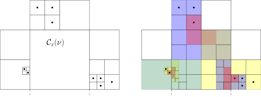
Figure 8: (Left) An empty cell $\mathcal{C}_{x}(\nu)$ in the initial quadtree $\mathcal{T}$ (Right) The subdivision of $\mathcal{C}_{x}(\nu)$ in the refined quadtree $\mathcal{T}^{\prime}$. (In this picture, we did not subdivide the other cells.)

Our AVD will consist of one region $V(\nu)$ for each node $\nu$ of $\mathcal{T}^{\prime}$:

• If $\nu$ is an ordinary, then the cell center $b(\nu)$ of the cell $\mathcal{C}(\nu)$ is the Voronoi region $V(\nu)$.

• If $\nu$ is a leaf node, then the Voronoi region $V(\nu)$ is the set of all the points $b(\mathcal{C}^{\prime})$ where $\mathcal{C}^{\prime}$ is either $\mathcal{C}(\nu)$ or a descendent of $\mathcal{C}(\nu)$. In other words, $V(\nu)$ is the set of all the points that are in or below $\mathcal{C}(\nu)$.

• If $\nu$ is a compressed node, let $\nu_{1}$ be its child. Then $V(\nu)$ is the set of all the points are on or below $\mathcal{C}(\nu)$, and are not on or below $\mathcal{C}(\nu_{1})$.

Preprocessing.

We denote by $b(\nu)$ the center of the quadtree box stored at node $\nu$, so we have $b(\nu)=b(\mathcal{C}(\nu))$. We first compute, for every node $\nu$ of $\mathcal{T}^{\prime}$, the point $h(\nu)$ in $P$ with highest $z$-coordinate that is recorded in the subtree rooted at $\nu$. (Again, we break ties by taking the point $p_{i}$ with smallest index $i$ among these highest points.) We can compute all these points in linear time by traversing the tree $\mathcal{T}^{\prime}$ from bottom to top.

Next we compute the $d_{2}$-nearest neighbor $n_{2}(\nu)=n_{2}(b(\nu))$ for all the nodes $\nu$ of $\mathcal{T}^{\prime}$. We compute these points by traversing the tree from top to bottom, so when we compute $n_{2}(\nu)$, we already know $n_{2}(\nu^{\prime})$ where $\nu^{\prime}$ is the parent of $\nu$. Let $\rho$ be the $d_{2}$-shortest path from $b(\nu)$ to $n_{2}(\nu)$. There are 4 cases:

1. If $n_{2}(\nu)=n_{2}(\nu^{\prime})$, then we are done as we already know $n_{2}(\nu^{\prime})$.

2. If $\rho$ is a downward path, then $n_{2}(\nu)=h(\nu)$.

3. If $\rho$ starts with a horizontal move from $b(\nu)$, then $n_{2}(\nu)$ is $h(\nu^{\prime})$ for some node $\nu^{\prime\prime}$ such that $\mathcal{C}(\nu^{\prime\prime})$ is a horizontal neighbor of $\mathcal{C}(\nu)$. So we can find $n_{2}(\nu)$ in $2^{O(D)}$ time.

4. Otherwise, $\rho$ first goes upward from $b(\nu)$, then follows a bridge $r^{\prime}r^{\prime\prime}$, and then goes downward to $n_{2}(b(\nu))$. As $n_{2}(\nu)\neq n_{2}(\nu^{\prime})$, it follows that $\nu^{\prime}$ is a compressed node. Then $\mathcal{C}(r^{\prime\prime})$ is not stored in $\mathcal{T}^{\prime}$, because if it were the case, we would have created a node for $\mathcal{C}(r^{\prime})$ in $\mathcal{T}^{\prime}$. So $r^{\prime\prime}$ is in $V(\nu^{\prime\prime})$ for some compressed node $\nu^{\prime\prime}$, and we have $n_{2}(b(\nu))=h(\nu^{\prime\prime})$. As $\mathcal{C}_{x}(\nu^{\prime})$ and $\mathcal{C}_{x}(\nu^{\prime\prime})$ must be adjacent, and due to the refinement phase, the size of $\mathcal{C}_{x}(\nu^{\prime})$ is smaller than the size of $\mathcal{C}_{x}(\nu^{\prime\prime})$, there are $2^{O(D)}$ candidates for $\nu^{\prime\prime}$, so we can find it in $2^{O(D)}$ time.

Finding the representative points.

We now explain how we choose the representative points for each region $V(\nu)$. For each node $\nu$, we pick $n_{2}(\nu)$ as a representative point. If $\nu$ is an ordinary cell, then we do not add any other representative point.

If $\nu$ is a leaf node or a compressed node, then for each compressed node $\nu^{\prime\prime}$ such that $\mathcal{C}_{x}(\nu^{\prime\prime})$ is adjacent to $\mathcal{C}_{x}(\nu)$, we add $h(\nu^{\prime\prime})$ as a representative point. By the same argument as in the above 4th case, there are at most $2^{O(D)}$ such points, and for each point $q$ in $V(\nu)$, either one of these points $h(\nu^{\prime\prime})$ or $n_{2}(\nu)$ is $n_{2}(q)$.

Results.

As $\mathcal{T}^{\prime}$ records $2^{O(D)}n$ nodes, it can be computed in $2^{O(D)}n\log n$ time, and it can be queries in $2^{O(D)}\log n$ time. So we obtained the following result:

Theorem 19.

Let $P$ be a subset of $\mathbb{B}^{D}$ of size $n$. Then we can compute in $2^{O(D)}n\log n$ time an AVD of $P$ with $2^{O(D)}n$ regions, and $2^{O(D)}$ representative points per region. Using this diagram, given a query point $q\in\mathbb{H}^{D}$, a point $n_{2}(q)\in P$ such that $d_{2}(q,n_{2}(q))$ is minimum can be returned in $2^{O(D)}\log n$ time.

We can also use this data structure to return an additive approximate nearest neighbor with respect to $d_{1}$, as $d_{1}(q,n_{2}(q))\leqslant d_{2}(q,n_{2}(q))+2$ by Theorem 6:

Corollary 20.

Let $P$ be a subset of $\mathbb{B}^{D}$ of size $n$. Then we can compute in $2^{O(D)}n\log n$ time an AVD of $P$ with $2^{O(D)}n$ regions, and $2^{O(D)}$ representative points per region. Using this diagram, given a query point $q$, we can return in $2^{O(D)}\log n$ time a point $n_{2}(q)\in P$ such that $d_{1}(q,n_{2}(q))\leqslant d_{1}(q,n_{1}(q))+2$, where $n_{1}(q)$ is a point in $P$ such that $d_{1}(q,n_{1}(q))$ is minimum.

Our discrete AVD can also be turned into an AVD for a set of points $P$ in $H^{D}$, by constructing the $d_{2}$-AVD for the points $\{b(p):p\in P\}$, and replacing each point $p$ in a Voronoi region by the whole box $\mathcal{C}(p)$, and thus we obtain a partition of $\mathbb{B}^{D}$. Then for a query point $q\in H^{D}$, we return a point in $P$ such that $b(p)=n_{2}(b(q))$. Theorem 14 implies that this point is an $O(\log D)$ additive approximate near neighbor:

Corollary 21.

Let $P$ be a subset of $\mathbb{H}^{D}$ of size $n$. Then we can compute in $2^{O(D)}n\log n$ time an AVD of $P$ with $2^{O(D)}n$ regions, and $2^{O(D)}$ representative points per region. Using this diagram, for any query point $q$, we can return in $2^{O(D)}\log n$ time a point $r\in P$ such that $d_{H}(q,r)\leqslant d_{H}(q,n_{H}(q))+O(\log D)$, where $n_{H}(q)$ is a the point in $P$ such that $d_{1}(q,n_{H}(q))$ is minimum.

References

- [1] Ingo Althöfer, Gautam Das, David P. Dobkin, Deborah Joseph, and José Soares. On sparse spanners of weighted graphs. Discret. Comput. Geom., 9:81–100, 1993. doi:10.1007/BF02189308.
- [2] Sunil Arya, Gautam Das, David M. Mount, Jeffrey S. Salowe, and Michiel H. M. Smid. Euclidean spanners: short, thin, and lanky. In Proc. 27th ACM Symposium on Theory of Computing, pages 489–498, 1995. doi:10.1145/225058.225191.
- [3] James Cannon, William Floyd, Richard Kenyon, and Walter Parry. Hyperbolic geometry. In Silvio Levy, editor, Flavors of Geometry, volume 31, pages 167–196. MSRI Publications, 1997.
- [4] Victor Chepoi, Feodor F. Dragan, Bertrand Estellon, Michel Habib, Yann Vaxès, and Yang Xiang. Additive spanners and distance and routing labeling schemes for hyperbolic graphs. Algorithmica, 62(3-4):713–732, 2012. doi:10.1007/s00453-010-9478-x.
- [5] Octavian Ganea, Gary Becigneul, and Thomas Hofmann. Hyperbolic neural networks. In S. Bengio, H. Wallach, H. Larochelle, K. Grauman, N. Cesa-Bianchi, and R. Garnett, editors, Advances in Neural Information Processing Systems, volume 31. Curran Associates, Inc., 2018. URL: https://proceedings.neurips.cc/paper_files/paper/2018/file/dbab2adc8f9d078009ee3fa810bea142-Paper.pdf.
- [6] M. Gromov. Hyperbolic Groups, pages 75–263. Springer New York, 1987.
- [7] Sariel Har-peled. Geometric Approximation Algorithms. American Mathematical Society, 2011.
- [8] Sándor Kisfaludi-Bak. A Quasi-Polynomial Algorithm for Well-Spaced Hyperbolic TSP. In Proc. 36th International Symposium on Computational Geometry (SoCG 2020), pages 55:1–55:15, 2020.
- [9] Sándor Kisfaludi-Bak and Geert van Wordragen. A quadtree for hyperbolic space, 2023. arXiv:2305.01356.
- [10] Robert Krauthgamer and James R. Lee. Algorithms on negatively curved spaces. In 2006 47th Annual IEEE Symposium on Foundations of Computer Science (FOCS’06), pages 119–132, 2006. doi:10.1109/FOCS.2006.9.
- [11] Sofya Raskhodnikova. Transitive-closure spanners: A survey. In Oded Goldreich, editor, Property Testing - Current Research and Surveys, volume 6390 of Lecture Notes in Computer Science, pages 167–196. Springer, 2010. doi:10.1007/978-3-642-16367-8\_10.
- [12] Y. Shavitt and T. Tankel. On the curvature of the internet and its usage for overlay construction and distance estimation. In IEEE INFOCOM 2004, volume 1, page 384, 2004. doi:10.1109/INFCOM.2004.1354510.
- [13] Mikkel Thorup. Parallel shortcutting of rooted trees. J. Algorithms, 23(1):139–159, 1997. doi:10.1006/jagm.1996.0829.