Balanced Resonate-and-Fire Neurons

Abstract

The resonate-and-fire (RF) neuron, introduced over two decades ago, is a simple, efficient, yet biologically plausible spiking neuron model, which can extract frequency patterns within the time domain due to its resonating membrane dynamics. However, previous RF formulations suffer from intrinsic shortcomings that limit effective learning and prevent exploiting the principled advantage of RF neurons. Here, we introduce the balanced RF (BRF) neuron, which alleviates some of the intrinsic limitations of vanilla RF neurons and demonstrates its effectiveness within recurrent spiking neural networks (RSNNs) on various sequence learning tasks. We show that networks of BRF neurons achieve overall higher task performance, produce only a fraction of the spikes, and require significantly fewer parameters as compared to modern RSNNs. Moreover, BRF-RSNN consistently provide much faster and more stable training convergence, even when bridging many hundreds of time steps during backpropagation through time (BPTT). These results underscore that our BRF-RSNN is a strong candidate for future large-scale RSNN architectures, further lines of research in SNN methodology, and more efficient hardware implementations.

1 Introduction

Artificial neural networks (ANNs) have become the main method for solving machine learning problems in recent years (Goodfellow et al., 2016; Wu & Feng, 2018; Abiodun et al., 2019). However, they require massive computation and energy, making them inefficient for large-scale real-world applications—particularly in the realm of edge computing—due to the deep non-linear continuous estimators to represent features of the data (Pfeiffer & Pfeil, 2018). Spiking neural networks (SNNs) circumvent this drawback by processing information through the precise timing of action potentials, or spikes. SNNs can potentially be more efficient compared to ANNs due to their event-driven property, for which computation is only required when spikes are propagated in the system (Paugam-Moisy & Bohté, 2012). Furthermore, SNNs are self-recurrent, as the neurons have a dynamic internal state that modulates their activity over time, and are more biologically realistic than conventional ANNs. Some examples of spiking neurons with ascending biological plausibility include the leaky integrate-and-fire (LIF) neuron, the adaptive leaky integrate-and-fire (ALIF) neuron (Bellec et al., 2018), the Izhikevich neuron (Izhikevich, 2003), and the Hodgkin-Huxley (HH) neuron (Hodgkin & Huxley, 1952). While the HH model is too computationally expensive for practical application, it exhibits rich and complex membrane dynamics that simpler models lack.

One mode of dynamics overlooked in ML applications in particular is the resonating behavior seen in oscillatory neurons. Subthreshold oscillations of the membrane potential have been observed in various mammalian nervous systems, including the neurons in the frontal cortex (Llinas et al., 1991), in the thalamus (Pedroarena & Llinás, 1997), and in layer II of the medial entorhinal cortex (Alonso & Llinás, 1989), which is crucial in spatial information processing (Doeller et al., 2010). The resonate-and-fire (RF) neuron proposed by Izhikevich (2001) models such damped or sustained subthreshold oscillations of biological neurons: the RF neuron fires when the frequency of the incoming spikes matches that of the neuron’s damped oscillation. Incoming signals with higher frequency leads to more firing for a LIF neuron but less firing for an RF neuron with slow oscillation. As the RF neuron is similarly computationally efficient as the LIF neuron, it is potentially a spiking neuron model suitable for large-scale SNNs (Izhikevich, 2001).

Previous works showed RF neurons implemented in the Intel Loihi 2 (Davies et al., 2018), a neuromorphic processor, can be used to compute the short-time Fourier transform (STFT) of signals (Frady et al., 2022) more computationally efficient than conventional STFT (Shrestha et al., 2023). Moreover, the RF neurons successfully converted raw data signals to spike trains, further input to SNNs with LIF neurons for detection and classification tasks (Hille et al., 2022; Lehmann et al., 2023). RF neurons have also been implemented in the framework of (feedforward) SNNs as harmonic oscillators for image classification tasks (AlKhamissi et al., 2021), as well as in optical flow estimation and audio classification tasks (Frady et al., 2022). Still, the performance of the RF models did not significantly exceed that of deep LIF SNNs (Frady et al., 2022) or LSTM cells (AlKhamissi et al., 2021), and these studies did not compare with state-of-art spiking neuron models, such as ALIF. Moreover, they lack of meaningful parameter studies and did not address stability issues of the vanilla RF model. Considering the strengths of the RF neuron, these results suggest that the full potential of the RF neuron has yet to be explored.

Recent methodological advances in training recurrent SNNs (RSNNs) have demonstrated their potential for effective time series learning, particularly in combination with BPTT (Bellec et al., 2018; Yin et al., 2021). Nonetheless, they do face a “convergence dilemma”—it requires usually up to many hundreds of epochs for RSNNs to converge properly (Yin et al., 2021; Fang et al., 2021; Zhang et al., 2023).

Here we propose a novel spiking neuron model—the balanced RF neuron—which overcomes both, the intrinsic limitations of vanilla RF neurons as well as shortcomings that arise during training of ALIF-RSNNs. As a result, our RF variants achieve not only comparable and higher task performance than the ALIF networks, but also remarkably fast and stable convergence, reaching 95% of the mean final accuracy within the first five epochs with up to seven times less spikes than ALIF networks.

2 Resonate-and-Fire Neurons

The oscillatory behavior of the membrane potential in an RF neuron is formulated with two linear differential equations:

$$\dot{x} =b\,x-\omega\,y+I$$ (1)

$$\dot{y} =\omega\,x+b\,y$$ (2)

which is expressed as a single complex equation:

$$\dot{u}=(b+i\,\omega)\,u+I$$ (3)

with $u=(x+i\,y)\in\mathbb{C}$ and $I$ the injected current (Izhikevich, 2001). $\omega>0$ is the angular frequency of the neuron, which describes how many radians the neuron progresses per second. $b<0$ is the dampening factor that exponentially decays the oscillation. The smaller $b$ is, the faster the oscillation dampens to the resting state.

Izhikevich RF Neuron.

We applied the Euler method (Atkinson, 1989) to Equation 3 with step size (time scale) $\delta$:

$$u(t)=u(t-\delta)+\delta\,((b+i\,\omega)\,u(t-\delta)+I(t))$$ (4)

which is used to simulate the RF neuron in Figure 1. It shows the oscillatory behavior when similar frequency-timed input is injected into an RF neuron with an angular frequency of 10 $rad/s$ and a dampening factor of -1.

Figure 1: Membrane dynamics of two RF neurons. The four excitatory input spikes are in phase with the neuron’s angular frequency $\omega=10$. The inhibitory spike at half-phase enhances the sensitivity of the neuron to forthcoming excitatory input. Depending on its parameterization, the neuron exhibits divergence behavior (top) with $b=-0.3$ and $\delta=0.01$ or convergence behavior (bottom) with $b=-1$. $I(t)\in\mathbb{R}$ and $u_{1}(t),u_{2}(t)\in\mathbb{C}$ refer to the injected current and the membrane potential of the neuron, respectively.

Harmonic RF Neuron.

In the harmonic RF (HRF) neuron, the membrane potential changes based on the dynamics of dampened harmonic oscillation (AlKhamissi et al., 2021). Instead of using a complex representation, the membrane potential is split into two states as follows:

$$\dot{u} =-2b\,u-\omega^{2}\,v+I$$ (5)

$$\dot{v} =u$$ (6)

By applying Euler integration we get the equations for discrete time steps:

$$\begin{split}u(t)&=u(t-\delta)+\delta(-2b\,u(t-\delta)\\ &\qquad-\omega^{2}v(t-\delta)+I(t))\end{split}$$ (7)

$$v(t) =v(t-\delta)+\delta u(t-\delta).$$ (8)

Here, $b>0$ is the dampening factor, and $\omega>0$ is the angular frequency.

3 Balanced RF Models

Initial exploration of the RF neurons in RSNN with a random subset of 32 samples from the sequential MNIST dataset (Deng, 2012) showed excessive spiking, divergent behavior, and the traditional hard and soft reset (Equation 23) hindering immediate resonance behavior.

Divergence is due to the approximation of the dynamic system in discrete steps and is dependent on the combination of $\omega$, $b$, and the discrete-time scale $\delta$, as shown in Figure 1 (top). The membrane potential diverges and continuously produces spikes unrelated to the input signal, causing noise and artificial signals that disrupt the original frequencies, which may have hindered effective learning of the model.

Balanced Izhikevich RF Neuron.

Considering the intrinsic limitations of the basic RF neuron, we introduce the balanced RF (BRF) neuron with a variation in the threshold, reset mechanism, and divergence boundary. To reduce continuous spiking of the neuron and induce spiking sparsity, a refractory period, referred to as $q(t)$, is implemented in the threshold, increasing it after a neuron fires:

$$\vartheta(t) =\vartheta_{c}+q(t)$$ (9)

$$z(t) =\Theta\,(\operatorname{Re}(u(t))-\vartheta(t))$$ (10)

with $\vartheta_{c}$ the constant threshold and $z(t)$ the output spiking. The real part of the Equation 3 was considered for the threshold mechanism, as it induces an immediate response. The refractory period decays exponentially with time:

$$q(t)=\gamma q(t-\delta)+z(t-\delta)$$ (11)

The default refractory period constant is $\gamma=0.9$.

Another limitation of the basic RF model was the traditional reset mechanism, which reduces the amplitude but disrupts the oscillation. Hence, we propose the smooth reset as an alternative that temporarily increases the dampening of the amplitude to decay faster after the neuron fires by means of integrating the refractory period into the dampening term:

$$b(t)=b_{c}-q(t)$$ (12)

with $b_{c}$ the constant dampening factor.

The influence of implementing the refractory period and the smooth reset can be seen in Figure 2. The single RF neuron was simulated with $\omega=10,\,b=-1$, and the input signal was frequency-timed. The combination of refractory period and smooth reset significantly reduced the number of spikes, while the output spikes effectively reflected the period of the angular frequency of the neuron. Without both, the RF neuron was not able to release single spikes but tended to burst.

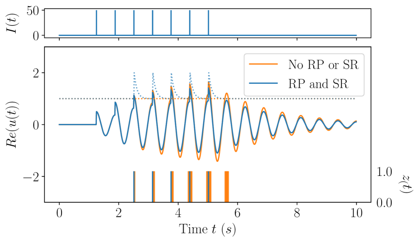
Figure 2: Membrane potential $u(t)$ and spiking response $z(t)$ of an RF neuron without refractory period (RP) or smooth reset (SR) (orange) compared to both (blue) for the given input signal $I(t)$.

To alleviate the divergence problem, we propose to restrict the parameter space to a subspace below the divergence boundary—an analytically derived relationship between $\delta$, $b_{c}$, and $\omega$ that ensures convergence. For an RF neuron to converge or show sustained oscillation, the magnitude of the membrane potential decreases or stays constant with time given an incoming signal:

$$|u(t)|\leq|u(t-\delta)|$$ (13)

After spike onset the magnitude converges—but does not precisely become 0, $|u(t-\delta)|\neq 0$, thus both side is divisible by $|u(t-\delta)|$

$$\frac{|u(t)|}{|u(t-\delta)|}\leq 1$$ (14)

Furthermore, the explicit form of the subthreshold oscillatory behavior of the membrane potential after an incoming spike is derived in Appendix A.3 and given as:

$$u(t)=\delta\,(1+\delta(b_{c}+i\,\omega))^{\frac{t}{\delta}-1}$$ (15)

The refractory period and the reset are not considered in the derivation, as post-spiking behavior is irrelevant for modeling subthreshold behavior. The explicit form is further implemented into the inequality above and simplified:

$$|1+\delta(b_{c}+i\,\omega)|\leq 1$$

$$\iff \sqrt{(1+\delta b_{c})^{2}+(\delta\omega)^{2}}\leq 1$$

Since the radicand is positive, both sides of the inequality can be squared:

$$\Longrightarrow(1+\delta b_{c})^{2}+(\delta\omega)^{2}-1\leq 0$$ (16)

The condition for the neuron to show damped oscillation is found by solving the quadratic inequality for $b_{c}$, where $b_{c}$ is in the following range of the solutions given a constant $\omega$:

$$\frac{-1-\sqrt{1-(\delta\,\omega)^{2}}}{\delta}<b_{c}<\frac{-1+\sqrt{1-(\delta\,\omega)^{2}}}{\delta}$$ (17)

Furthermore, the neuron is a sustained oscillator if:

$$b_{c}=\frac{-1\pm\sqrt{1-(\delta\,\omega)^{2}}}{\delta}$$ (18)

which leads us to another condition of the neuron, since $b_{c}\in\mathbb{R}_{<0}$ and $\omega\in\mathbb{R}_{>0}$:

$$\sqrt{1-(\delta\,\omega)^{2}}>0\Rightarrow\omega\leq\frac{1}{\delta}$$ (19)

With a default $\delta=0.01$, the highest frequency that the neuron can resonate at is the frequency corresponding to an angular frequency of $100~{}rad/s$. We define this angular frequency as the upper boundary $\omega_{ub}$. The upper bound of $b_{c}$ that leads to sustained oscillation is implemented in this paper as $p(\omega)$, also considered the divergence boundary:

$$p(\omega)=\frac{-1+\sqrt{1-(\delta\,\omega)^{2}}}{\delta}$$ (20)

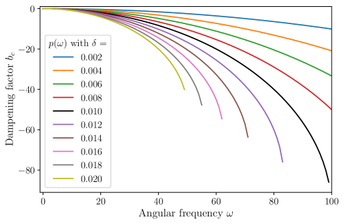
Figure 9: Divergence boundary depending on $\delta\in\{0.002,\cdots,0.02\}$

combined with a trainable b-offset $b^{\prime}>0$ to ensure flexibility and convergence $b_{c}=p(\omega)-b^{\prime}$ which is constant throughout one sequence length. Figure 9 shows exemplary divergence boundaries for various $\delta$ values. By combining the derived dampening factor with the smooth reset, we present the final equation of $b(t)$ used in this paper:

$$b(t)=p(\omega)-b^{\prime}-q(t)$$ (21)

Implementing the refractory period, smooth reset, and the divergence boundary to efficient learning and sparse spiking for all four datasets.

Balanced Harmonic RF Neuron.

Similarly, we propose the balanced HRF (BHRF) neuron with the refractory period, smooth reset, and a tailored divergence boundary for $b$ depending on $\omega$:

$$p(\omega)=\frac{\omega^{2}}{200}$$ (22)

For $\delta=0.01$ and $b_{c}=p(\omega)$, the BHRF neuron shows sustained oscillation.

Frequency Response of the BRF Neuron.

The frequency response plots shown in Figure 3 assess how well the RF neuron responds to specific frequencies. A peak on a frequency response plot indicates a high sensitivity of the neuron to the input signal frequency (details in Appendix A.4). The figure shows alignment of the response peak and $\omega$ of the RF neuron, demonstrating the resonance property to also be present in the discrete case. The slight offset of the response peak and $\omega$ of the RF neuron is an artifact of the numerical integration of the membrane dynamics’ differential equation and disappears with decreasing the temporal step size $\delta$.

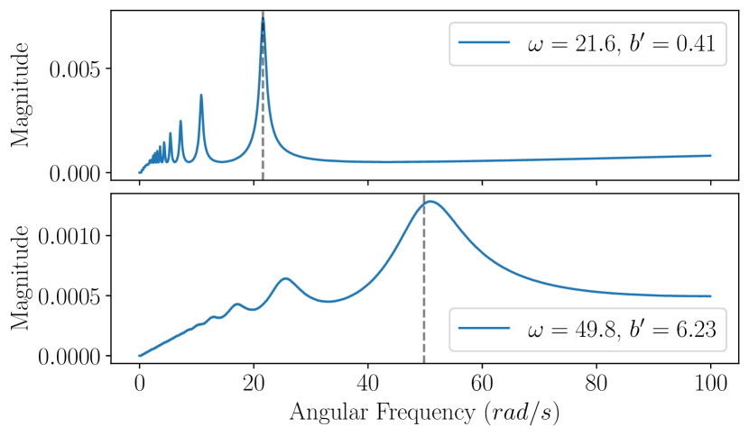
Figure 3: RF neuron frequency response plots for exemplary omega $\omega$ and b-offset $b^{\prime}$ combinations with $\delta=0.001$.

The RF neuron can also be considered a narrow band pass filter, for which only a specific range of frequencies are filtered depending on its angular frequency. Combined with the discrete time scale and b-offset, they determine how narrow and sensitive the band pass filter is. At a global scale, the RF neuron can also be considered a low pass filter, as it can only filter frequencies below the corresponding angular frequency $\omega_{ub}$ (Equation 19).

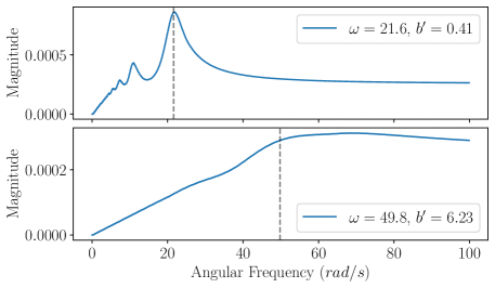
Figure 8: HRF neuron frequency response plots for exemplary omega $\omega$ and b-offset $b^{\prime}$ combinations with $\delta=0.001$.

We focused on the BRF neuron and the BHRF remained preliminary in its exploration, as the BRF responses were more sensitive to the input frequencies than BHRF responses shown in Figure 8.

4 Network Implementation

We implement the BRF and BHRF neurons into the RSNN and applied them to simulations with several benchmark datasets. The essential formulations of the BRF and BHRF neuron are summarized in Algorithm 1 and Algorithm 2, respectively. Note that for the algorithmic formulation we change the notation to time-discrete tensor operations and superscript the time index, whereas the transition from $t$ to $t+1$ is considered as a time delay of $\delta$.

Algorithm 1 BRF Forward Pass

$\mathbf{b}^{t}=p(\boldsymbol{\omega})-\mathbf{b}^{\prime}-\mathbf{q}^{t-1}$
$\mathbf{u}^{t}=\mathbf{u}^{t-1}+\delta((\mathbf{b}^{t}+i\boldsymbol{\omega})\,\mathbf{u}^{t-1}+\mathbf{x}^{t})$
$\boldsymbol{\vartheta}^{t}=\vartheta_{c}+\mathbf{q}^{t-1}$
$\textbf{z}^{t}=\Theta(\operatorname{Re}(\textbf{u}^{t})-\boldsymbol{\vartheta}^{t})\\$ $\mathbf{q}^{t}=\gamma\mathbf{q}^{t-1}+\mathbf{z}^{t}$
 
$\vartheta_{c}=1$, $\gamma=0.9$, and $p(\boldsymbol{\omega})=\frac{-1+\sqrt{1-(\delta\,\boldsymbol{\omega})^{2}}}{\delta}$
($\operatorname{Re}$, $\Theta$, $p$ are applied component-wise.)

Algorithm 2 BHRF Forward Pass

$\mathbf{b}^{t}=p(\boldsymbol{\omega})-\mathbf{b}^{\prime}-\mathbf{q}^{t-1}$
$\mathbf{u}^{t}=\mathbf{u}^{t-1}+\delta(-2\mathbf{b}^{t}\mathbf{u}^{t-1}-\boldsymbol{\omega}^{2}\mathbf{v}^{t-1}+\mathbf{x}^{t})$
$\mathbf{v}^{t}=\mathbf{v}^{t-1}+\delta\mathbf{u}^{t-1}$
$\boldsymbol{\vartheta}^{t}=\vartheta_{c}+\mathbf{q}^{t-1}$
$\textbf{z}^{t}=\Theta(\textbf{u}^{t}-\boldsymbol{\vartheta}^{t})\\$ $\mathbf{q}^{t}=\gamma\mathbf{q}^{t-1}+\mathbf{z}^{t}$
 
$\vartheta_{c}=1$, $\gamma=0.9$, and $p(\boldsymbol{\omega})=\frac{\boldsymbol{\omega}^{2}}{200}$
($\operatorname{Re}$, $\Theta$, $p$ are applied component-wise.)

We trained the networks with BPTT with the double-Gaussian function (Equation 38, Yin et al., 2021) as the surrogate gradient (Neftci et al., 2019). Further details of the networks are described in Appendix A.6.

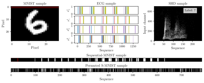
Figure 4: Overview over the datasets. Examplary MNIST image and its corresponding sequential and permuted representations. Common pixel row outlined in red on MNIST and S-MNIST sample. ECG sample after level cross encoding. SHD sample after preprocessing.

5 Experiments

The MNIST dataset consists of grayscale 28$\times$28 pixel hand-written digit images for classification. The sequential-MNIST (S-MNIST), which converts the image to a sequence of 1 $\times$ 784, is a prominent benchmark dataset that enable comparison between sequential models with 54,000 images for training, 6,000 for validation, and 10,000 for testing. In the permuted S-MNIST variant (PS-MNIST), the pixel positions were first permuted randomly and then kept fixed.

Electrocardiogram (ECG) recordings of the heart are represented in voltage over time and consist of cyclic activity with six characteristic waveforms: P, PQ, QR, RS, ST, and TP. The QT database consisted of ECG recordings with per-time step labels classified by experts in the field (Laguna et al., 1997). There were 105 recordings, each recorded for 15 minutes with two electrodes. We left out 24 signals, as they were sudden death recordings without annotation. For the preprocessing shown in Figure 4, refer to Section A.7 in the appendix.

The Spiking Heidelberg dataset (SHD) is a benchmark audio-to-spike dataset specifically generated for SNNs (Cramer et al., 2020). It contains 10,420 recordings of spoken digits from 0 to 9 in English and German. The recordings were made with high fidelity and then converted into spike trains for 700 channels through a precise artificial inner ear model (Cramer et al., 2020). The spike trains were further processed with a discrete time scale of 4e-3 s to obtain sequence length of 250 with zero-padding. This preprocessing was conducted to make the dataset comparable to Yin et al. (2021). We used 7,341 sequences for training, 815 for validation, and 2,264 for inference.

6 Results

Table 1: Results between vanilla RF, BRF, BHRF, ALIF (Yin et al., 2021), and other SoTa models: DCLS-Delays (DCLS-D) (Hammouamri et al., 2023) and RadLIF (Bittar & Garner, 2022) on various sequential classification tasks. Architecture represents the number of neurons in each layer. The average accuracy over five runs shown for the RF, BRF and BHRF models, excluding PS-MNIST BHRF. SOPs: average spike operations. ^*RSNN-SoTa ^**SNN-SoTa

Task	Model	Architecture	No. params. ($\downarrow$)	Test Acc. ($\uparrow$)	SOPs ($\downarrow$)	SOPs/step ($\downarrow$)	SOP Ratio ($\downarrow$)
S-MNIST	ALIF*	4,64,$(256)^{2}$,10	156,126	98.7 %	70,810.8	90.32	1.00$\times$
	RF	1,256,10	68,874	98.0$\pm 0.4~{}\%$	29,034.8	37.03	0.41$\times$
	BRF	1,256,10	68,874	99.0$\pm 0.1~{}\%$	15,462.6	19.72	0.22$\times$
	BHRF	1,256,10	68,874	99.1$\pm 0.1~{}\%$	21,565.7	25.51	0.30$\times$
PS-MNIST	ALIF*	4,64,$(256)^{2}$,10	156,126	94.3 %	59,772.1	76.24	1.00$\times$
	RF	1,256,10	68,874	9.9$\pm 0.8~{}\%$	66,474.2	84.79	1.11$\times$
	BRF	1,256,10	68,874	95.0$\pm 0.2~{}\%$	27,839.7	35.51	0.46$\times$
	BHRF	1,256,10	68,874	95.2 %	24,564.2	33.33	0.41$\times$
ECG	ALIF*	4,36,6	1,776	85.9 %	35,011.2	26.93	1.00$\times$
	RF	4,36,6	1,734	85.4$\pm 0.5~{}\%$	11,966.9	9.21	0.34$\times$
	BRF	4,36,6	1,734	85.8$\pm 0.7~{}\%$	6,307.7	4.85	0.18$\times$
	BHRF	4,36,6	1,734	87.0$\pm 0.4~{}\%$	6,233.8	4.80	0.18$\times$
SHD	DCLS-D**	700,$(256)^{2}$,20	$\approx$200,000	95.1$\pm 0.2~{}\%$	-	-	-
	RadLIF*	700,$(1024)^{3}$,20	3,893,288	94.62$\%$	-	-	-
2-8[2pt/1pt]	ALIF	700,$(128)^{2}$,20	142,120	90.4 %	24,690.0	98.76	1.00$\times$
	RF	700,128,20	108,820	90.4$\pm 0.7~{}\%$	4,691.7	18.77	0.19$\times$
	BRF	700,128,20	108,820	91.7$\pm 0.8~{}\%$	3,502.6	14.01	0.14$\times$
	BHRF	700,128,20	108,820	92.7$\pm 0.7~{}\%$	4,139.5	16.56	0.17$\times$

The results, the network architecture, the number of parameters, and the number of produced spikes, between the best-performing BRF- and BHRF-RSNN and the baseline ALIF-RSNNs (see Section A.2) or other state-of-the-art (SoTa) models, are compared for each classification task in Table 1. The BHRF and BRF models outperformed the RSNN SoTa for three and two tasks respectively. Complementing accuracy, we also find that much enhanced sparseness in the BRF and BHRF networks while using substantially fewer parameters compared to the ALIF networks.

We also compare the theoretical energy efficiency of the RF and ALIF models as by computing their respective total spiking operations (SOPs) (Equation 40) and SOPs per sequence step. As both measures were considerably smaller for the BRF and BHRF models, this implies they require less computation to achieve better or comparable performance. This may be due to the resonating spiking behavior of the neuron, needing fewer spikes to represent its frequency, as well as the refractory period and smooth reset that hinders continuous spiking. A particularly large difference was seen in the SHD task, where the BRF model spiked only 14% of the ALIF model. Compared to the standard RF model, our balanced variants achieved significantly sparser activity while obtaining higher performance. Especially for the PS-MNIST, the standard RF model stayed at chance, while our balanced RF variations outperformed RSNN-SoTA.

Overall, we find that RSNNs comprised of either BRF and BHRF neurons exceeded performance for all classification tasks compared to the baseline ALIF-RSNN. Compared to standard RF neurons, the smooth reset, refractory period, and divergence boundary significantly improved the stability and learning of the RF parameters, possibly exploiting the model’s resonant properties. We study this in detail below.

Table 2: Quantitative convergence results. The average number of epochs after which $95\,\%$, $98\,\%$, and $100\,\%$ of the final test accuracy on the learning curve was reached, respectively.

Task	Model	$\mathbf{95\,\%}$ ($\downarrow$)	$\mathbf{98\,\%}$ ($\downarrow$)	$\mathbf{100\,\%}$ ($\downarrow$)
S-MNIST	ALIF	105	162	276
	BRF	3	29	246
	BHRF	5	12	119
PS-MNIST	ALIF	143	200	265
	BRF	10	39	282
	BHRF	6	19	123
ECG	ALIF	51	157	282
	BRF	5	31	75
	BHRF	15	38	109
SHD	ALIF	14	15	16
	BRF	2	3	7
	BHRF	3	5	8

Convergence.

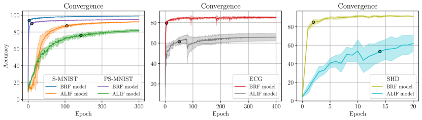
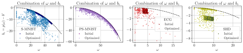
Figure 5: Top row: S-MNIST, PS-MNIST, ECG, and SHD learning curve between BRF and ALIF model. Each curve averaged per epoch (solid line) with standard deviation (shaded area) over five runs. The dot on the accuracy curves depict the point at which 95 % of the final accuracy was reached. Bottom row: S-MNIST, PS-MNIST, ECG, and SHD initial and optimized BRF parameter combinations: angular frequency $\omega$ and b-offset $b^{\prime}$ for all runs. Dashed line is the divergence boundary.

The learning curves of the BRF and ALIF models are presented in Figure 5. We reduced the ALIF model to the same size and number of trainable parameters as the BRF model. For the S-MNIST and PS-MNIST tasks, the ALIF networks only learned effectively when the truncated BPTT (TBPTT) with truncation step 50 was applied. Nonetheless, the fully back-propagated BRF networks converged significantly faster than the TBPTT ALIF networks, also evident from the quantitative convergence results (Table 2). The BRF networks showed especially stable convergence, as the five runs converged with only a small standard deviation. A similar pattern of fast and stable convergence was observed for the ECG dataset and SHD.

While numerically large, the learning rates of the BRF-RSNNs led to stable and fast convergence for most datasets. This is in contrast to standard SNNs where large learning rates lead to poor performance. Here, the double-Gaussian surrogate gradient function (Yin et al., 2021) we used may have contributed by ensuring gradient flow even for neurons far from firing. Combined with the high learning rate, this may have enabled non-spiking neurons to effectively shift their angular frequencies.

The ECG task was learned most effectively for the BRF and BHRF networks with a small batch size and high learning rate. A smaller batch size captures detailed variations within the dataset, notably the timing of the input spikes, which may have been important for per-step wave classification.

Parameter analysis.

We also compared the trainable BRF parameters $\omega$ and $b^{\prime}$ between the initial and trained networks to obtain an intuition of the functioning of the neuron, as shown in Figure 5. We see that optimization substantially shifted the parameters, demonstrating that the gradients in the B(H)RF networks were effectively propagated.

For the S-MNIST task, plotting $\omega$-$b_{c}$ (Figure 5) shows clusters around $\omega$ values of 18 to 28 $rad/s$ and around $\omega$ of 40 $rad/s$ with a wide range of $b_{c}$. The dampening factor close to zero indicates near-sustained oscillation behavior, preserving resonance amplitude for an extended duration. The clustered variety in $b_{c}$ values suggests that short- and long-term memory are essential for effective learning of the S-MNIST task in B(H)RF networks. Additionally, the distribution of $\omega$ for S-MNIST task showed a bimodal distribution with the highest peak at 23.3 to 25.3 $rad/s$ and the second peak at 40.8 to 42.8 $rad/s$. The MNIST digits all contain some form of diagonal line with a width of 3 to 6 pixels, most prominently observed in digit 1. When converted into a sequence row-by-row, the lines are distributed among the sequence with a periodic signal of about 25 pixels. Considering the pixels as discrete time steps of $\delta$ = 0.01, the theoretical period T frequently observed in the signal is T = 0.25 $s$. Thus, the most frequent theoretical angular frequency $\omega^{\prime}$ underlying the signal is around $\omega^{\prime}=2\pi/0.25\,s=25.13~{}rad/s$ which is close to the most frequently learned angular frequencies of the BRF neuron. This simple calculation thus suggests that the BRF neurons were able to learn meaningful frequencies that underlie the S-MNIST dataset. For the PS-MNIST, we see more spread of $\omega$ and $b_{c}$ parameters, as the specific optimal frequency in S-MNIST is removed by the permutation.

Inspecting spike train ECG samples (Figure 4), we observe distinguishable periodic spikes with 300 time step intervals, corresponding to a theoretical angular frequency of $\omega^{\prime}=2.09$ $rad/s$, and indeed a cluster at about 2 $rad/s$ is present in the $\omega$-$b_{c}$ plot. The theoretical and optimized angular frequencies aligned, demonstrating learning of the dynamical signal by the network.

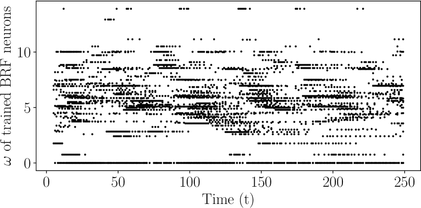
Figure 6: Raster plot of network activity for an SHD sample with label 10 after training. The BRF neurons are sorted by their angular frequency. Black dots denote output spikes.

Weight Sparsity.

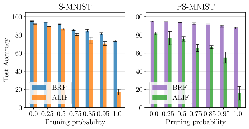
Figure 7: Test accuracy vs pruning probability for (a) S-MNIST and (b) PS-MNIST. 1.0 pruning indicate no recurrent weights.

We explored the effect of pruning recurrent weights in an ablation study for the S-MNIST and PS-MNIST tasks between comparable BRF and ALIF networks, as detailed in Table 4 and LABEL:app:psmnist_lc_hyp. Results are shown in Figure 7, where the BRF neuron provides constant performance throughout pruning, while the ALIF model performs poorly when lacking recurrent weights. This demonstrates that explicit recurrencies were not necessary for the BRF networks with resonating properties to learn well, while these connections were crucial for the ALIF networks. Moreover, the BRF networks’ accuracy had a smaller standard deviation throughout compared to the ALIF networks, also showing that the BRF network performance was not affected by the specific pruned weights as much as the ALIF networks.

7 Discussion

The results from our BRF-RSNN implementation lead to considerable insight into the workings of the RF neurons. Importantly, the learning curve and parameter analyses of the datasets show that the BRF networks learned meaningful parameters by favorably tuning the resonating behavior, modeling the complex dynamics not yet observed in large-scale simulations. We observe favorable oscillatory behavior of the membrane potential and increasing frequency of periodic spikes with higher angular frequency in the raster plot for all datasets. For SHD, output spikes are present towards the end of the sequence, even with the zero padding of the input signal. As most signals are still periodic, it suggests controlled oscillation and spiking that maintained relevant frequencies until the end of the sequence.

Note that we conducted the experiments without biases for all RF models to see how many spikes are needed to keep the network dynamics alive and to solve the tasks. As a result, a few of the BRF neurons in the network learned to fire consistently throughout the sequence as seen in Figure 6 and thus “imitated” a bias injecting constant current into the network. In contrast, ALIF networks need explicit biases to perform well. The BRF networks are thus more flexible in modeling behavior that cannot be learned by the integrator neurons alone.

8 Conclusion

We introduced BRF- and BHRF-RSNNs as a principled resonating spiking neuron model that solves the training difficulties encountered for networks comprised of standard RF neurons while demonstrating the effectiveness of internal resonating state as a form of long-term memory. Our BRF- and BHRF-RSNNs with smaller network architectures and sparser spiking outperformed and yielded results comparable to the deep baseline models. The learning curves showed that the BRF models converged faster than the ALIF models. Furthermore, the stable convergence hints at good reproducibility of the BRF model given the hyperparameters. The BRF parameter analyses displayed indications of the network to learn frequencies underlying the input signals and showed resilience against sparser recurrent connections compared to the ALIF network.

One drawback of our BRF- and BHRF-RSNNs was the difficulty in finding an optimal initial parameterization of the angular frequencies and the dampening factor offset, since both determine the models’ performance, The analyses of the parameters introduced the possibility of applying the Fourier transform on the datasets a-priori to approximate the range of angular frequencies the BRF neurons requires to optimally learn the data.

Like ALIF networks, the BRF-RSNNs required extensive time for training due to the custom implementation in PyTorch; one training period of the S-MNIST and PS-MNIST, for example, took 20 to 30 hours with a NVIDIA GeForce RTX 2080 Ti, similar to the ALIF single-layered model. The training period was shorter compared to the deep-layered ALIF networks, but still remains a challenge. Nonetheless as shown in the results, faster convergence enabled earlier stopping of training with acceptable performance if a short training period was required, for example, in practical applications.

Possible future research may be to scale up the simulations to much larger and more complex problems, such as the CIFAR (Krizhevsky & Hinton, 2009) or the Google Speech Command dataset (Warden, 2018). It is of particular interest to apply the BRF model to raw audio processing task, because of its ability to extract periodic pattern within the time domain.Moreover, applying trainable refractory period or completely adaptive threshold may be fascinating.

This study was an initial exploration to investigate the working of resonating neurons in the recurrent spiking neuron framework. Our networks showed comparable results and exceeded the state-of-the-art for RSNNs. We see many possible approaches to extending our work, as the implementation was kept to its simplest form. The presented work thus provided a foundation for further exploration of the BRF-RSNN variants.

Appendix A Appendix

A.1 Traditional soft and hard reset

The traditional reset mechanism considered was formulated as the following:

$$u(t)=(1-\zeta\,z(t))\,u^{\prime}(t)$$ (23)

for which the $u^{\prime}(t)$ represent the membrane potential before reset and $\zeta\in(0,1]$ the amount of reset, where $\zeta=1$ led to a hard reset, otherwise soft.

A.2 Baseline ALIF neuron

The formulation of the baseline ALIF neuron (Yin et al., 2021) is as follows with $\vartheta=0.01$ and $\beta=1.8$:

$$\vartheta^{t}=\vartheta+\beta\,a(t)$$ (24)

$$a(t)=\rho\,a(t-\delta)+(1-\rho)\,z(t-\delta)$$ (25)

$$u^{\prime}(t)=\alpha\,u(t-\delta)+(1-\alpha)\,I(t)$$ (26)

$$z(t)=\Theta\,(u^{\prime}(t)-\vartheta^{t})$$ (27)

$$u(t)=u^{\prime}(t)-z(t)\,\vartheta^{t}$$ (28)

where $\rho=e^{-\frac{\delta}{\tau_{a}}}\in(0,1)$ is the adaptive threshold decay constant, $\tau_{a}$ the time constant and $\alpha=e^{-\frac{\delta}{\tau_{m}}}\in(0,1)$ the membrane potential decay constant. $a(t)$ is the accumulative activity of the spiking behavior of the neuron. The membrane potential $u(t)$ is soft reset with the adaptive threshold $\vartheta^{t}$ when the neuron fires ($z(t)=1$).

A.3 Explicit form of the Izhikevich RF neuron

We can reform the membrane equation to $u(t)=(1+\delta\,(b+i\,\omega))\,u(t-\delta)+\delta\,I(t)$. Consider discrete time step $\delta$ with t = 0, $\delta$, $2\delta$, $3\delta,\,,T\delta$. Assume a spike injected only at $t=\delta$ with $I(\delta)=1$ and initial membrane potential $u(0)=0$, then:

$$u(\delta) =\delta$$ (29)

$$u(2\delta) =\delta\,(1+\delta\,(b+i\,\omega))$$ (30)

$$u(3\delta) =(1+\delta\,(b+i\,\omega))(\delta\,(1+\delta\,(b+i\,\omega)))$$ (31)

$$=\delta\,(1+\delta\,(b+i\,\omega))^{2}$$ (32)

$$u(4\delta) =(1+\delta\,(b+i\,\omega))(\delta\,(1+\delta\,(b+i\,\omega))^{2})$$ (33)

$$=\delta\,(1+\delta\,(b+i\,\omega))^{3}$$ (34)

$$\cdots$$ (35)

$$u(t) =\delta\,(1+\delta\,(b+i\,\omega))^{\frac{t}{\delta}-1}$$ (36)

A.4 Frequency response plot generation

The subthreshold responses were explored with randomly chosen angular frequency $\omega\in[0,100)$ and $b^{\prime}\in(0,10)$ for the RF neurons. Spiking input signals with frequencies relative to the angular frequencies of $\{0.1,0.2\cdots,100\}$ were input to the neurons over 20 seconds with a discrete-time scale of $\delta=0.001$. The positive spikes were input in-phase of the period corresponding to the angular frequency:

$$T=\frac{2\pi}{\text{angular frequency}}$$ (37)

The mean absolute magnitude of the membrane potential over the whole sequence was calculated and plotted to get the response of the neuron per tested frequency signal. Similarly conducted for the HRF neurons.

A.5 Divergence Boundary

The discrete-time scale $\delta$ has a large impact on the divergence behavior. Figure below shows the curve of divergence boundary for time scales above and below the default $\delta=0.01$. The membrane potential converges if the combination of $\omega$ and $b_{c}$ is below the line. When considering the $\omega$ range of 0 to 100 $rad/s$, the slope of the sustained oscillation curve becomes flatter with smaller $\delta$. The more precise the oscillation is modeled, the less likely the system will diverge. Indeed, the discrete approximation of the continuous differential equation becomes more precise by computing smaller time scales.

A.6 Experimental Setup

The fully recurrent RF-RSNN with $m$ input, $h$ hidden BRF or BHRF, and $C$ leaky integrator (LI) output neurons was computed using PyTorch (Paszke et al., 2017). The backpropagation through time (BPTT) algorithm with minibatch size $B$ was used with the Adam (Kingma & Ba, 2014), RAdam (Liu et al., 2020), or the RMSprop (Hinton et al., 2012) depending on the network and task. The input from the current sequence step $\mathbf{x}^{t}\in\mathbb{M}_{B\times m}$ and the output spiking of the recurrent hidden neurons from the previous time step $\mathbf{z}^{t-1}\in\mathbb{M}_{B\times h}$ were combined by implementing a fully connected linear layer. This combined signal $\mathbf{x}^{t}\in\mathbb{M}^{B\times h}$ corresponded to the familiar injected current $I(t)$ but was written in matrix form to represent all hidden neurons in the minibatch. Although not explicit in the Algorithms, $\mathbf{w_{in,rec}}\in\mathbb{M}_{h\times(m+h)}$ and $\mathbf{w_{out}}\in\mathbb{M}_{C\times h}$ represent the strength of the connections between the input-to-hidden, hidden-to-hidden, and hidden-to-output neurons, which were optimized. No biases were trained or used in the network. The B(H)RF neurons with $\boldsymbol{\omega}$ and $\mathbf{b^{\prime}}\in\mathbb{R}^{h}$ were updated over the time sequence of $B$ data samples with $\mathbf{u}^{t},(\mathbf{v}^{t}),\mathbf{b}^{t},\mathbf{q}^{t},\boldsymbol{\vartheta}^{t}\in\mathbb{M}_{B\times h}$. The LI membrane potential time decay constant $\boldsymbol{\tau_{m,out}}\in\mathbb{R}_{>0}^{C}$ was also learned. The negative log-likelihood (NLL) or the cross-entropy (CE) loss was implemented as our criterion depending on the simulations.

For the ALIF implementation, the adaptive threshold time decay constant $\boldsymbol{\tau_{a}}\in\mathbb{R}_{>0}^{h}$ is additionally learned with the membrane potential time decay constant $\boldsymbol{\tau_{m}}\in\mathbb{R}_{>0}^{h}$.

In the case of average sequence loss with NLL, the logarithmic softmax function was computed for all output neurons per time step $\mathbf{\hat{y}}^{t}=log(\text{softmax}(\mathbf{u}^{t}_{out}))$, which was further propagated into the loss function: $\mathcal{L}^{t}=\text{criterion}(\mathbf{\hat{y}}^{t},\mathbf{y}^{t})=\frac{1}{B}\sum_{c=1}^{C}-y^{t}_{c}\,\hat{y}^{t}_{c}$ where $\mathbf{y}^{t}\in\mathbb{M}_{B\times C}$ is the target label at time step $t$ represented as one-hot vectors. The mean loss was computed as $\mathcal{L}=\frac{1}{T}\sum^{T}_{t=1}\mathcal{L}^{t}$ with sequence length T. In the case of label-last loss, only the loss from the last time step was propagated backwards.

The backward pass of the BPTT algorithm was internally computed with the automatic differentiation engine in PyTorch (Paszke et al., 2017). For the non-differentiable Heaviside function in the B(H)RF and ALIF neurons, the multi-Gaussian function (Yin et al., 2021) was manually implemented as the surrogate gradient (Neftci et al., 2019):

$$\frac{\partial\Theta}{\partial u}=_{def}(1+h)g(u,\vartheta,\sigma)-2hg(u,\vartheta,s\sigma)$$ (38)

with

$$g(x,\mu,\sigma)=e^{-\frac{1}{2}\left(\frac{x-\mu}{\sigma}\right)^{2}}$$ (39)

with $h{=}0.15$, $s{=}6$, $\sigma{=}0.5$ similar to Yin et al. (2021). The negative gradient values were motivated by the leaky rectified and exponential linear unit that prevented the “dying-ReLU” problem (Lu et al., 2019). With these values, the multi-Gaussian surrogate gradient function promoted the neurons to spike despite an initial low membrane potential, which contributed to effective learning.

The best model was the model saved with the highest average test loss over the first five runs by early stopping on the validation loss. The loss and accuracy of the train, validation, and test set were logged into Tensorboard (Abadi et al., 2016) for analysis of the learning pattern. After obtaining the best model, the spiking operations (SOPs) were computed based on the five saved models by taking the total number of output spikes over the whole dataset $z_{sum}$ with respect to the number of data samples $N$:

$$\operatorname{SOPs}=\frac{z_{sum}}{N}$$ (40)

The results were compared with the baseline ALIF-RSNN.

For simulating the models and performing the experiments, we used multiple systems with different deep learning accelerators including NVIDIA GeForce RTX 2060, NVIDIA GeForce RTX 2080 Ti, NVIDIA GeForce RTX 3090, and NVIDIA A100, with PyTorch 2.0.1 on Python 3.10.4 and CUDA 11.7.

A.7 ECG-QT database preprocessing

The preprocessed QT data were extracted from Yin et al. (2021) to gain comparable results. The original sequences were segmented into smaller intervals, each containing 1300 ms of the recordings. Then, the two ECG signals were normalized and encoded into two separate spike trains via level-cross encoding. The positive gradients above and negative gradients below the threshold led to spikes with the threshold $L=0.3$:

$$s_{+} =\begin{cases}1&\text{if }x_{t}-x_{t-1}\geq L\\ 0&\text{otherwise}\end{cases}$$ (41)

$$s_{-} =\begin{cases}1&\text{if }x_{t}-x_{t-1}\leq-L\\ 0&\text{otherwise}\end{cases}$$ (42)

The target labels were segmented correspondingly and predicted for each time step. Figure 4 color: blue, red, green, cyan, olive and purple corresponds to the label: P, PQ, QR, RS, ST. Five hundred fifty-seven segments were used for training, 61 for validation, and 141 for testing.

A.8 Hyperparameters

Table 3: Sequential-MNIST hyperparameters applied for the best-performing BRF, HBRF, and ALIF model with label-last loss and truncation step of 50 for TBPTT (used to compare pruning). $\mathcal{U}(a,b)$: parameters sampled from a uniform distribution with range of $a$ to $b$. $\mathcal{N}(\mu,\sigma)$: parameters sampled from a normal distribution with mean $\mu$ and std $\sigma$.

Model	BRF-RSNN		BHRF-RSNN	ALIF-RSNN
	BPTT	TBPTT	BPTT	BPTT	TBPTT
Network	1 + 256 (fully recurrent) + 10		1 + 256 (fully recurrent) + 10	1 + 256 (fully recurrent) + 10
Learning rate (Lr)	0.1	0.006	0.1	0.001
Loss function	NLL		CE	NLL
Minibatch size	256		256	256
Lr scheduling	LinearLR		LinearLR	LinearLR
Optimizer	Adam		RAdam	Adam
Epochs	300		400	300
Parameter initialization	$\omega:\mathcal{U}(15,50)$ $b^{\prime}:\mathcal{U}(0.1,1)$ $\tau_{m,out}:\mathcal{N}(20,5)$		$\omega:\mathcal{U}(15,35)$ $b^{\prime}:\mathcal{U}(0.1,1)$ $\alpha:Sigmoid(\mathcal{N}(0,0.1))$	$\tau_{m}:\mathcal{N}(20,5)$ $\tau_{a}:\mathcal{N}(200,50)$ $\tau_{m,out}:\mathcal{N}(20,5)$

Table 4: Permuted S-MNIST hyperparameters applied for the best-performing BRF, HBRF, and ALIF model with average sequence loss and truncation step of 50 for TBPTT.

Model	BRF-RSNN		BHRF-RSNN	ALIF-RSNN
	BPTT	TBPTT	BPTT	BPTT	TBPTT
Network	1 + 256 (fully recurrent) + 10		1 + 256 (fully recurrent) + 10	1 + 256 (fully recurrent) + 10
Learning rate (Lr)	0.1	0.006	0.1	0.001
Loss function	NLL		NLL	NLL
Minibatch size	256		256	256
Lr scheduling	LinearLR		LinearLR	LinearLR
Optimizer	Adam		RAdam	Adam
Epochs	300		200	300
Parameter initialization	$\omega:\mathcal{U}(15,85)$ $b^{\prime}:\mathcal{U}(0.1,1)$ $\tau_{m,out}:\mathcal{N}(20,1)$		$\omega:\mathcal{U}(15,50)$ $b^{\prime}:\mathcal{U}(1,6)$ $\alpha:Sigmoid(\mathcal{N}(0,0.1))$	$\tau_{m}:\mathcal{N}(20,5)$ $\tau_{a}:\mathcal{N}(200,50)$ $\tau_{m,out}:\mathcal{N}(20,5)$

Table 5: ECG QT database hyperparameters applied for the best-performing BRF, HBRF, and ALIF model with truncation step of 50 for TBPTT.

Model	BRF-RSNN		BHRF-RSNN	ALIF-RSNN
	BPTT	TBPTT	BPTT	BPTT	TBPTT
Network	4 + 36 (fully recurrent) + 6		4 + 36 (fully recurrent) + 6	4 + 36 (fully recurrent) + 6
Learning rate (Lr)	0.1	0.004	0.3	0.05	0.002
Loss function	NLL		NLL	NLL
Minibatch size	16		4	64
Lr scheduling	LinearLR		LinearLR	LinearLR
Optimizer	Adam		RAdam	Adam
Epochs	400		300	400
Parameter initialization	$\omega:\mathcal{U}(3,5)$ $b^{\prime}:\mathcal{U}(0.1,1)$ $\tau_{m,out}:\mathcal{N}(20,1)$		$\omega:\mathcal{U}(7,11)$ $b^{\prime}:\mathcal{U}(0.1,1)$ $\alpha:Sigmoid(\mathcal{N}(0,0.1))$	$\tau_{m}:\mathcal{N}(20,0.5)$ $\tau_{a}:\mathcal{N}(7,0.2)$ $\tau_{m,out}:\mathcal{N}(20,0.5)$
Sub-seq. length	0		0	10

Table 6: Spiking Heidelberg dataset (SHD) hyperparameters applied for the best-performing BRF, HBRF, and ALIF model with average sequence loss and truncation step of 50 for TBPTT.

Model	BRF-RSNN		BHRF-RSNN	ALIF-RSNN
	BPTT	TBPTT	BPTT	BPTT	TBPTT
Network	700 + 128 (fully recurrent) + 20		700 + 128 (fully recurrent) + 20	700 + 128 (fully recurrent) + 20
Learning rate (Lr)	0.075	0.02	0.1	0.075	0.02
Loss function	NLL		NLL	NLL
Minibatch size	32		32	32
Lr scheduling	LinearLR		LinearLR	LinearLR
Optimizer	Adam		RMSprop	Adam
Epochs	20		20	20
Parameter initialization	$\omega:\mathcal{U}(5,10)$ $b^{\prime}:\mathcal{U}(2,3)$ $\tau_{m,out}:\mathcal{N}(20,5)$		$\omega:\mathcal{U}(3,10)$ $b^{\prime}:\mathcal{U}(0.1,1)$ $\alpha:Sigmoid(\mathcal{N}(0,0.1))$	$\tau_{m}:\mathcal{N}(20,5)$ $\tau_{a}:\mathcal{N}(150,10)$ $\tau_{m,out}:\mathcal{N}(20,5)$
Sub-seq. length	0		0	10

Due to the BHRF-RSNN being in the preliminary phase of its exploration, we initially used the Sigmoid function for the leaky integrator decay constant $\alpha$, as it ensured the decay to be in the range of 0 and 1.

References

- Abadi et al. (2016) Abadi, M., Agarwal, A., Barham, P., Brevdo, E., Chen, Z., Citro, C., Corrado, G. S., Davis, A., Dean, J., Devin, M., et al. Tensorflow: Large-scale machine learning on heterogeneous distributed systems. arXiv preprint arXiv:1603.04467, 2016.
- Abiodun et al. (2019) Abiodun, O. I., Jantan, A., Omolara, A. E., Dada, K. V., Umar, A. M., Linus, O. U., Arshad, H., Kazaure, A. A., Gana, U., and Kiru, M. U. Comprehensive review of artificial neural network applications to pattern recognition. IEEE access, 7:158820–158846, 2019.
- AlKhamissi et al. (2021) AlKhamissi, B., ElNokrashy, M., and Bernal-Casas, D. Deep spiking neural networks with resonate-and-fire neurons. arXiv preprint arXiv:2109.08234, 2021.
- Alonso & Llinás (1989) Alonso, A. and Llinás, R. R. Subthreshold na+-dependent theta-like rhythmicity in stellate cells of entorhinal cortex layer ii. Nature, 342(6246):175–177, 1989.
- Atkinson (1989) Atkinson, K. E. An introduction to numerical analysis, john wiley and sons. New York, 19781, 1989.
- Bellec et al. (2018) Bellec, G., Salaj, D., Subramoney, A., Legenstein, R., and Maass, W. Long short-term memory and learning-to-learn in networks of spiking neurons. Advances in neural information processing systems, 31, 2018.
- Bittar & Garner (2022) Bittar, A. and Garner, P. N. A surrogate gradient spiking baseline for speech command recognition. Frontiers in Neuroscience, 16:865897, 2022.
- Cramer et al. (2020) Cramer, B., Stradmann, Y., Schemmel, J., and Zenke, F. The heidelberg spiking data sets for the systematic evaluation of spiking neural networks. IEEE Transactions on Neural Networks and Learning Systems, 33(7):2744–2757, 2020.
- Davies et al. (2018) Davies, M., Srinivasa, N., Lin, T.-H., Chinya, G., Cao, Y., Choday, S. H., Dimou, G., Joshi, P., Imam, N., Jain, S., et al. Loihi: A neuromorphic manycore processor with on-chip learning. Ieee Micro, 38(1):82–99, 2018.
- Deng (2012) Deng, L. The mnist database of handwritten digit images for machine learning research. IEEE Signal Processing Magazine, 29(6):141–142, 2012.
- Doeller et al. (2010) Doeller, C. F., Barry, C., and Burgess, N. Evidence for grid cells in a human memory network. Nature, 463(7281):657–661, 2010.
- Fang et al. (2021) Fang, W., Yu, Z., Chen, Y., Masquelier, T., Huang, T., and Tian, Y. Incorporating learnable membrane time constant to enhance learning of spiking neural networks. In 2021 IEEE/CVF International Conference on Computer Vision (ICCV), pp. 2641–2651, 2021. doi: 10.1109/ICCV48922.2021.00266.
- Frady et al. (2022) Frady, E. P., Sanborn, S., Shrestha, S. B., Rubin, D. B. D., Orchard, G., Sommer, F. T., and Davies, M. Efficient neuromorphic signal processing with resonator neurons. Journal of Signal Processing Systems, 94(10):917–927, 2022.
- Goodfellow et al. (2016) Goodfellow, I., Bengio, Y., and Courville, A. Deep Learning. MIT Press, 2016. http://www.deeplearningbook.org.
- Hammouamri et al. (2023) Hammouamri, I., Khalfaoui-Hassani, I., and Masquelier, T. Learning delays in spiking neural networks using dilated convolutions with learnable spacings. arXiv preprint arXiv:2306.17670, 2023.
- Hille et al. (2022) Hille, J., Auge, D., Grassmann, C., and Knoll, A. Resonate-and-fire neurons for radar interference detection. In Proceedings of the International Conference on Neuromorphic Systems 2022, pp. 1–4, 2022.
- Hinton et al. (2012) Hinton, G., Srivastava, N., and Swersky, K. Neural networks for machine learning lecture 6a overview of mini-batch gradient descent. Cited on, 14(8):2, 2012.
- Hodgkin & Huxley (1952) Hodgkin, A. L. and Huxley, A. F. A quantitative description of membrane current and its application to conduction and excitation in nerve. The Journal of physiology, 117(4):500, 1952.
- Izhikevich (2001) Izhikevich, E. M. Resonate-and-fire neurons. Neural networks, 14(6-7):883–894, 2001.
- Izhikevich (2003) Izhikevich, E. M. Simple model of spiking neurons. IEEE Transactions on neural networks, 14(6):1569–1572, 2003.
- Kingma & Ba (2014) Kingma, D. P. and Ba, J. Adam: A method for stochastic optimization. arXiv preprint arXiv:1412.6980, 2014.
- Krizhevsky & Hinton (2009) Krizhevsky, A. and Hinton, G. Learning multiple layers of features from tiny images, 2009.
- Laguna et al. (1997) Laguna, P., Mark, R., Goldberger, A., and Moody, G. A database for evaluation of algorithms for measurement of qt and other waveform intervals in the ecg. Computers in Cardiology, 24(1):673–676, 1997.
- Lehmann et al. (2023) Lehmann, H. M., Hille, J., Grassmann, C., and Issakov, V. Direct signal encoding with analog resonate-and-fire neurons. IEEE Access, 2023.
- Liu et al. (2020) Liu, L., Jiang, H., He, P., Chen, W., Liu, X., Gao, J., and Han, J. On the variance of the adaptive learning rate and beyond. In Proceedings of the Eighth International Conference on Learning Representations (ICLR 2020), April 2020.
- Llinas et al. (1991) Llinas, R. R., Grace, A. A., and Yarom, Y. In vitro neurons in mammalian cortical layer 4 exhibit intrinsic oscillatory activity in the 10-to 50-hz frequency range. Proceedings of the National Academy of Sciences, 88(3):897–901, 1991.
- Lu et al. (2019) Lu, L., Shin, Y., Su, Y., and Karniadakis, G. E. Dying relu and initialization: Theory and numerical examples. arXiv preprint arXiv:1903.06733, 2019.
- Neftci et al. (2019) Neftci, E. O., Mostafa, H., and Zenke, F. Surrogate gradient learning in spiking neural networks: Bringing the power of gradient-based optimization to spiking neural networks. IEEE Signal Processing Magazine, 36(6):51–63, 2019.
- Paszke et al. (2017) Paszke, A., Gross, S., Chintala, S., Chanan, G., Yang, E., DeVito, Z., Lin, Z., Desmaison, A., Antiga, L., and Lerer, A. Automatic differentiation in pytorch. In NIPS-W, 2017.
- Paugam-Moisy & Bohté (2012) Paugam-Moisy, H. and Bohté, S. M. Computing with spiking neuron networks. Handbook of natural computing, 1:1–47, 2012.
- Pedroarena & Llinás (1997) Pedroarena, C. and Llinás, R. Dendritic calcium conductances generate high-frequency oscillation in thalamocortical neurons. Proceedings of the National Academy of Sciences, 94(2):724–728, 1997.
- Pfeiffer & Pfeil (2018) Pfeiffer, M. and Pfeil, T. Deep learning with spiking neurons: Opportunities and challenges. Frontiers in neuroscience, 12:774, 2018.
- Shrestha et al. (2023) Shrestha, S. B., Timcheck, J., Frady, P., Campos-Macias, L., and Davies, M. Efficient video and audio processing with loihi 2. arXiv preprint arXiv:2310.03251, 2023.
- Warden (2018) Warden, P. Speech commands: A dataset for limited-vocabulary speech recognition. arXiv preprint arXiv:1804.03209, 2018.
- Wu & Feng (2018) Wu, Y.-c. and Feng, J.-w. Development and application of artificial neural network. Wireless Personal Communications, 102:1645–1656, 2018.
- Yin et al. (2021) Yin, B., Corradi, F., and Bohté, S. M. Accurate and efficient time-domain classification with adaptive spiking recurrent neural networks. Nature Machine Intelligence, 3(10):905–913, 2021.
- Zhang et al. (2023) Zhang, S., Yang, Q., Ma, C., Wu, J., Li, H., and Tan, K. C. Long short-term memory with two-compartment spiking neuron. arXiv preprint arXiv:2307.07231, 2023.