Learning to Defer in Content Moderation:
The Human-AI Interplay

Abstract

Ensuring successful content moderation is vital for a healthy online social platform where it is necessary to responsively remove harmful posts without jeopardizing non-harmful content. Due to the high-volume nature of online posts, human-only moderation is operationally challenging, and platforms often employ a human-AI collaboration approach. A typical machine-learning heuristic estimates the expected harmfulness of incoming posts and uses fixed thresholds to decide whether to remove the post (classification decision) and whether to send it for human review (admission decision). This can be inefficient as it disregards the uncertainty in the machine-learning estimation, the time-varying element of human review capacity and post arrivals, and the selective sampling in the dataset (humans only review posts filtered by the admission algorithm).

In this paper, we introduce a model to capture the human-AI interplay in content moderation. The algorithm observes contextual information for incoming posts, makes classification and admission decisions, and schedules posts for human review. Non-admitted posts do not receive reviews (selective sampling) and admitted posts receive human reviews on their harmfulness. These reviews help educate the machine-learning algorithms but are delayed due to congestion in the human review system. The classical learning-theoretic way to capture this human-AI interplay is via the framework of learning to defer, where the algorithm has the option to defer a classification task to humans for a fixed cost and immediately receive feedback. Our model contributes to this literature by introducing congestion in the human review system. Moreover, unlike work on online learning with delayed feedback where the delay in the feedback is exogenous to the algorithm’s decisions, the delay in our model is endogenous to both the admission and the scheduling decisions.

We propose a near-optimal learning algorithm that carefully balances the classification loss from a selectively sampled dataset, the idiosyncratic loss of non-reviewed posts, and the delay loss of having congestion in the human review system. To the best of our knowledge, this is the first result for online learning in contextual queueing systems and hence our analytical framework may be of independent interest.

1 Introduction

Recent advances in Artificial Intelligence (AI) provide the promise of freeing humans from repetitive tasks by responsive automation, thus enabling the humankind to focus on more creative endeavors [Yeh23]. One example of automating traditionally human-centric tasks is content moderation targeting misinformation and explicitly harmful content in social platforms such as Facebook [Met23], Twitter [X C23], and Reddit [Red23]. Historically (e.g., forums in the 2000s), human reviewers would monitor all exchanges to detect any content that violated the community standards [Rob19]. That said, the high volume of posts in current platforms coupled with the advances in AI has led platforms to automate their content moderation, harnessing the responsiveness of AI. This trend of automating traditionally human-centric tasks applies broadly beyond content moderation; for example, speedy insurance claim process [Pin23] and domain-specific generative AI copilots [GO23].

However, excessive use of automation in such human-centric applications significantly reduces the reliability of the systems. AI models are trained based on historical data and therefore their predictions reflect patterns observed in the past that are not always accurate for the current task. On the other hand, humans’ cognitive abilities and expertise make humans more attune to correct decisions. In content moderation, particular posts may have language that is unclear, complex, and too context-dependent, obscuring automated predictions [Met22]. Similarly, AI models may wrongfully reject a valid insurance claim [Eub18] and Large Language Model copilots may hallucinate non-existing legal cases [Nov23]. These errors can have significant ethical and legal repercussions.

The learning to defer paradigm is a common way to combine the responsiveness of AI and the reliability of humans. When a new job arrives, the AI model classifies it as accept or reject, and determines whether to defer the job for human review by admitting it to a corresponding queue (in content moderation, incoming jobs correspond to new posts and the classification decision pertains to whether the post is kept on or removed from the platform). When a human reviewer becomes available, the AI model determines which job to schedule for human review. As a result, the AI model directly determines which posts will be reviewed by humans.

At the same time, humans also affect the AI model as their labels for the reviewed jobs form the dataset based on which the AI is trained, creating an interplay between humans and AI. Hence, the AI model’s admission decisions are not only useful for correctly classifying the current jobs but are also crucial for its future prediction ability, a phenomenon known as selective sampling.

Figure 1: Pipeline of human-AI interplay in content moderation

In this paper, we model this human-AI interplay in the context of content moderation (though our insights can be transferable to other human-centric settings) and pose the following question:

How can we make classification, admission, and scheduling decisions that
combine the responsiveness of AI and the reliability of humans?

1.1 Our contributions

Learning to defer with capacity constraints.

To formally tackle the problem, we introduce a model that combines learning to defer with soft capacity constraints via queueing delays. To the best of our knowledge, the impact of limited capacity for learning to defer has not been considered in the literature (see Section 1.2 for further discussion). In particular, in each period $t=1,\ldots,T$, a post $j$ arrives with a type $k(j)$ drawn from a time-varying distribution over $K$ types. A post $j$ has an unknown cost $c_{j}=h_{k(j)}+\xi_{j}$ where $\xi_{j}\sim\mathcal{N}(0,\sigma_{k(j)}^{2})$ is a zero-mean idiosyncratic Gaussian noise while $h_{k}$ and $\sigma_{k}^{2}$ are the expectation and variance of the cost of type-$k$ posts. To capture the difference in reliability, we assume that the AI model only observes the type of the post; the true cost $c_{j}$ is only observable via human reviews. To capture the impact of limited human capacity, we assume that posts that are admitted (deferred) by the AI wait in a review queue. At the end of a period, one post in the queue is scheduled for review; the review is completed in this period with a probability $\mu_{k}N(t)$ that depends on both the specific post type $k$ and the fluctuating capacity of reviewers $N(t)$. We assume that a type-$k$ post is viewed only within $\ell_{k}$ periods since its arrival and only if it is not removed.

We measure the loss of a policy by comparing it to an omniscient benchmark that keeps benign posts ($c_{j}\leq 0$) and removes harmful posts ($c_{j}>0$). Note that this omniscient benchmark is not limited by capacity, which means that we need a capacity-constrained benchmark to argue about the efficiency of our policies. As a result, we define the average regret of a policy by comparing its time-averaged loss to a fluid benchmark that incorporates time-varying capacity constraints.

Balancing idiosyncrasy loss with delays.

As typical in complex learning settings, we start by assuming knowledge of the latent parameters (i.e., the expected costs $h_{k}$). The classification decision is then to keep the post $j$ if and only if the expected cost of its type is negative: $h_{k(j)}<0$. Of course, deferring a post to human reviewers can improve upon this ex-ante classification decision as human reviewers can observe the true cost. The admission decision should thus identify the posts that would benefit the most from this more refined observation. If all types have equal variance then the human reviewing capacity is more efficiently allocated when it focuses on borderline posts, i.e., $h_{k(j)}$ close to $0$, as borderline types have higher probability that the true cost of their posts has a different sign from their expected cost (which would lead to a different classification by the omniscient benchmark). This intuition drives the design of admission policies in existing content moderation practice [MSA⁺21, ABB⁺22] that operate based on two thresholds: a post $j$ is rejected (resp. accepted) without admission if its expected cost $h_{k(j)}$ is above the higher (resp. below the lower) threshold and is admitted for human review if it lies between the two thresholds. A more detailed comparison to these works is provided in Appendix A.

That said, even when all expected costs $h_{k}$ are known, there are two important shortcomings in these two-threshold heuristics. First, when the variance of different types is heterogeneous, the admission decision should not be restricted to the expected costs but rather also take variance into account. In particular, it may be more beneficial to defer to human reviewers post from a non-borderline type $k$ with high idiosyncratic variance $\sigma_{k}^{2}$ instead of wasting human capacity on more deterministic borderline types. Second, even if we operate with variance-aware scores, using static thresholds does not allow the system to adapt to the time-varying arrival patterns of posts and the fluctuating human capacities that arise in practice (see [MSA⁺21, Figure 2]). In particular, in certain time periods, the number of borderline posts may be either too large resulting in high delays for admitted posts due to the overflow in the review system or too small resulting in misclassification for some non-borderline posts that could have been prevented if they were admitted.

Our approach (Section 3) quantifies and balances the two losses hinted above (due to idiosyncrasy and delay) and is henceforth called Balanced Admission Control for Idiosyncrasy and Delay or BACID as a shorthand. We first calculate the expected ex-ante per-period loss of keeping a post on the platform (resp. removing it) using the distributional information of the true cost $c_{j}$; this loss is denoted by $r_{k}^{O}$ (resp. $r_{k}^{R}$). Hence, if a post is not admitted to human review, its per-period loss is $r_{k}=\min(r_{k}^{O},r_{k}^{R})$ and thus its idiosyncrasy loss that aggregates over its lifetime is $r_{k}\ell_{k}$. On the other hand, admitting a post incurs delay loss, which is the increase in congestion for future posts due to the limited human capacity. Motivated by the drift-plus-penalty literature [Nee22], we estimate the delay loss of a post by the number of posts of the same type currently waiting for reviews. We then admit a post if (a weighted version of) its idiosyncrasy loss (which one can avoid by admission) exceeds the estimated delay loss (which occurs due to the admission). For scheduling, we choose in each period the type with the most number of waiting posts (weighted by the difficulty to review this type) to review. We show that while heuristics like AI-Only or Human-Only have average regret at least $\Omega(\ell_{\max})$ (Propositions 1 and 2), where $\ell_{\max}$ is the maximum lifetime, BACID achieves a $O(\sqrt{K\ell_{\max}})$ average regret even with general time-varying arrivals and capacities (Theorem 1). This bound is optimal on the dependence on $\ell_{\max}$ as we also show a lower bound $\Omega(\sqrt{\ell_{\max}})$ for any deterministic policy (Theorem 2).

Efficient learning with selective sampling, optimism and forced scheduling.

To deal with unknown expected costs $h_{k}$, a typical approach in the bandit literature is to use an optimistic estimator for the unknown quantities. The unknown quantity that affects our admission rule is $r_{k}$, which depends on the unknown expected cost $h_{k}$. Following the optimistic approach, we first create a confidence interval $[\underline{h}_{k},\bar{h}_{k}]$ for the unknown expected cost $h_{k}$ based on reviewed posts. We then compute an optimistic estimator $\bar{r}_{k}$ using the parameter $\widetilde{h}_{k}\in[\underline{h}_{k},\bar{h}_{k}]$ that maximizes $r_{k}(\widetilde{h}_{k})$.The optimistic admission rule then admits a new post if (a weighted version of) the optimistic idiosyncrasy loss, $\bar{r}_{k}\ell_{k}$, exceeds its estimated delay loss. The high-level idea behind optimism is that, if a post is admitted (due to the optimistic estimation), we collect additional samples for this post which result in shrinking the confidence interval and eventually leading the confidence interval to converge to the true parameter $h_{k}$. Without considering heterogeneity in variance, [ABB⁺22] adopts a similar optimism-only heuristic to address the online learning nature of $h_{k}$.

However, optimism-only learning heuristics disregard the selective sampling nature of the feedback. When there is uncertainty on $h_{k}$, the benefit of admitting a post is not restricted to avoiding the idiosyncrasy loss of the current post, but extends to having one more data points that can improve the classification decision of future posts. This benefit does not arise when $h_{k}$ is known because the best classification decision is then clear (keep a post if and only if $h_{k}\leq 0$). With unknown $h_{k}$, there is an additional classification loss due to incorrect estimation of the sign of $h_{k}$. Given that optimism-only heuristics emulate the admission rule with known $h_{k}$, they disregard this classification loss and more broadly the positive externality that labels for the current post have on future posts. This challenge highlights that optimism-only heuristics such as Upper Confidence Bound (UCB) do not employ forward-looking exploration but rather optimistically myopic exploitation. They are myopic in their nature: they create a confidence interval around the parameter of interest and are optimistic with respect to this confidence interval, but they make an exploit decision based on those optimistic estimates. Concretely, given the most optimistic estimates about the underlying parameters, these algorithms select the action that myopically maximizes the contribution of the current post without actively considering any positive externality of the labels on future posts. We formally illustrate this inefficiency of optimism-only learning heuristics in Proposition 3.

To circumvent the above issue, we design an online learning version of BACID (Section 4) , which we term OLBACID, that augments the optimistic admission with label-driven admission and forced scheduling. When a post arrives, we estimate its potential classification loss based on its current confidence interval; if this is higher than a threshold, we admit the post to a label-driven queue and prioritize posts in this queue via forced scheduling to ensure enough labels for future classification decisions. To avoid exhausting human capacity, we limit the number of posts in the label-driven queue to one at any time. We show that OLBACID enjoys an average regret of $\tilde{O}(\sqrt{K\ell_{\max}}+K\ell_{\max}/\sqrt{T})$ (Theorem 3), addressing the inefficiency of optimism-only heuristics.

Context-defined types with type aggregation and contextual learning.

To remove the dependence on $K$, which can be large when types are defined based on contextual information (e.g., word embeddings of the contents), we provide a contextual bandit extension of our algorithm. In particular, we consider a linear contextual setting where $h_{k}=\boldsymbol{\phi}_{k}^{\intercal}\boldsymbol{\theta}^{\star}$ where $\boldsymbol{\phi}_{k}$ is a known $d-$dimensional feature vector for each type $k$ and $\boldsymbol{\theta}^{\star}$ is an unknown $d-$dimensional vector; this linear cost structure is similar to the one used in [ABB⁺22].

Our contextual extension (Section 5), which we term COLBACID, addresses the two facets where the previous algorithms require dependence on the number of types $K$. First, recall that BACID estimates the delay loss of admitting a post by the number of same-type posts in the review system. This naturally creates a dependence on the number of types $K$. Instead, we aggregate types into $G$ groups such that any two types $k,k^{\prime}$ in the same group satisfy $|\mu_{k}-\mu_{k^{\prime}}|\leq\Delta$ for some parameter $\Delta$. This aggregation enables us to estimate the delay loss by the number of same-group waiting posts, thus removing the aforementioned dependence on $K$. Second, recall that the learning in OLBACID creates a separate confidence interval for each type and refining those intervals introduces a dependence on $K$. By employing techniques from the linear contextual bandit literature [APS11], we replace this dependence with the dimension $d$. We note that our setting has the additional complexity that the feedback is received after a queueing delay which is endogenous to the admission and scheduling decisions of the algorithm (see Appendix D.1 for a comparison to contextual bandit with delays where delays are assumed to be exogenous). To handle this challenge, our scheduling employs a first-come-first-serve review order for posts in the same group and we only use data from the same group to estimate the expected cost of a type, which controls the delay by the number of same-group posts in the review system.

Our instance-dependent guarantee $\tilde{O}(\sqrt{G\ell_{\max}}+\ell_{\max}(\Delta+d\sqrt{G/T})$ (Theorem 4) scales optimally with the maximum lifetime $\ell_{\max}$ and avoids the dependence on $K$. We also provide a worst-case guarantee $\tilde{O}(\ell_{\max}^{2/3}+\ell_{\max}^{7/6}d/\sqrt{T})$ with no dependence on $G$ and $\Delta$ at the cost of a worse dependence on $\ell_{\max}$ (Corollary 1). To the best of our knowledge, this is the first result for online learning in contextual queueing systems and hence our analytical framework may be of independent interest.

1.2 Related work

Human-AI collaboration.

The nature of human-AI collaboration can be broadly classified into two types: augmentation and automation [BM17, RK21]. In particular, augmentation represents a “human-in-the-loop” type workforce where human experts combine machine learning with their own judgement to make better decisions. Such augmentation is often found in high-stake settings such as healthcare [LLL22], child maltreatment hotline screening [DFC20], refugee resettlement [BP22, AGP⁺23] and bail decisions [KLL⁺18]. A general concern for augmentation relates to humans’ compliance patterns to [BBS21, LLL22], the impact of such patterns to decision accuracy [KLL⁺18, MS22] and the impact on fairness [MSG22, GBB23]. Automation, on the other hand, concerns the use of machine learning in place of humans and is widely applied in human and social services where colossal demands overwhelm limited human capacity, such as in data labelling [VLSV23], content moderation [GBK20, MSA⁺21] and insurance [Eub18]. Full automation is clearly undesirable in these applications as machine learning can err. A natural question is how one can better utilize the limited human capacity when machine is uncertain about the prediction. The literature on “learning to defer”, which studies when machine learning algorithms should defer decisions to downstream experts, tries to answer this question and is where our work fits in.

Assuming that humans have perfect prediction ability but there is limited capacity, classical learning to defer has two streams of research, learning with abstention and selective sampling. Although these two streams have been studied separately (with a few exceptions, see discussion below), our work provides an endogenous approach to connect them. In particular, learning with abstention can be traced back to [Cho57, Cho70] and studies an offline classification problem with the option to not classify a data point for a fixed cost. For example, in content moderation, this corresponds to paying a fixed fee to an exogenous human reviewer to review a post. Since optimizing the original problem is computational infeasible, an extensive line of work investigates suitable surrogate loss functions and optimization methods; see [BW08, EW10, CDM16] and references therein. For online learning with expert advice, it is shown that even a limited amount of abstention allows better regret bound than without [SZB10, LLWS11, ZC16, NZ20]; [CDG⁺18] studies a similar problem but allows experts to also abstain. Selective sampling (or label efficient prediction) considers a different model where the algorithm makes predictions for every arrival; but the ground truth label is unavailable unless the algorithm queries for it; if queried, the label is available immediately [CLS05]. The goal is to obtain low regret while using as few queries possible. Typical solutions query only when a confidence interval exceeds a certain threshold [CLS05, CBGO09, OC11, DGS12]. There is recent work connecting the two directions by showing that allowing abstention of a small fixed cost can lead to better regret bound for selective sampling [ZN22, PZ22]. However, these works treat the abstention cost and selective sampling exogenously. Existing work neglects the impact of limited human capacity to learning to defer[LSFB22]. Our model serve as one step to capture it by endogenously connecting both costly abstention and selective sampling via delays. In particular, our admission component determines both abstention and selective sampling. In addition, the cost of abstention is dynamically affected by the delay in getting human reviews whereas the avoidance of frequent sampling (to get data) is captured by its impact on the delay.

Although the above line of work as well as ours assumes perfect labels from human predictions, a more recent stream of work on “learning to defer” considers imperfect human predictions and is focused on combining prediction ability of experts and learning algorithms; this moves towards the augmentation type of human-machine collaboration. In particular, [MCPZ18, MS20, WHK20, CMSS22] study a setting with an offline dataset and expert labels. The goal is to learn both a classifier, which predicts outcome, and a rejector that predicts when to defer to human experts. The loss is defined by the machine’s classification loss over non-deferred data, humans’ classification loss over deferred data, and the cost to query experts. [DKGG20, DOZR21] study a setting where given expert loss functions, the algorithm picks a size-limited subset of data to outsource to humans and solves a regression or a classification problem on remaining data, with a goal to minimize the total loss. [RBC⁺19] extends the model by allowing the expert classification loss to depend on human effort and further considering an allocation of human effort to different data points. [KLK21, VBN23, MMZ23] consider learning to defer with multiple experts.

Bandits with knapsacks or delays.

Restricting our attention to admission decisions, our model bears similar challenges with the literature on bandits with knapsacks or broadly online learning with resource constraints, which finds applications in revenue management [BZ12, WDY14, FSW18]. In particular, for bandits with knapsacks, there are arrivals with rewards and required resources from an unknown distribution. The algorithm only observes the reward and required resources after admitting an arrival and the goal is to obtain as much reward as possible subject to resource constraints [BKS18, AD19]. A typical primal-dual approach learns the optimal dual variables of a fixed fluid model and explores with upper confidence bound [BLS14, LSY21]; these extend to contextual settings [WSLJ15, AD16, ADL16, SSF23], general linear constraints [PGBJ21, LLSY21] and constrained reinforcement learning [BDL⁺20, Che19]. These results cannot immediately apply to our setting for two reasons. First, the resource constraint in our model is dynamically captured by time-varying queue lengths instead of a single resource constraint over the entire horizon; thus learning fixed dual variables is insufficient for good performance. Second, our admission decisions must also consider the effect on classification; thus relying only on optimism-based exploration is insufficient (see Section 4.1).

The problem of bandits with delays is related to our setting where feedback of an admitted post gets delayed due to congestion. Motivated by conversion in online advertising, bandits with delays consider the problem where the reward of each pulled arm is only revealed after a random delay independently generated from a fixed distribution [DHK⁺11, Cha14]. Assuming independence between rewards and delays as well as bounded delay expectation, [JGS13, MLBP15] propose a general reduction from non-delay settings to their delayed counterpart. Subsequent papers consider censored settings with unobservable rewards [VCP17], general (heavy-tail) delay distributions [MVCV20, WW22] and reward-dependent delay [LSKM21]. [VCL⁺20, BXZ23] study (generalized) linear contextual bandit with delayed feedback. The key difference between bandits with delays and our model is that delays for posts in our model are not independent across posts due to queueing effect; we provide a more elaborate comparison to those works in Appendix D.1.

Learning in queueing systems.

Learning in queueing systems can be classified into two types: 1) learning to schedule with unknown service rates to obtain low delay; 2) learning unknown utility of jobs / servers to obtain high reward in a congested system. For the first line of research, an intuitive approach to measure delay suboptimality is via the queueing regret, defined as the difference in queue lengths compared with a near-optimal algorithm [WX21]. The interest for queueing regret is in its asymptotic scaling in the time horizon, and it is studied for single-queue multi-server systems [Wal14, KSJS21, SSM21], multi-queue single-server systems [KAJS18], load balancing [CJWS21], queues with abandonment [ZBW22] and more general markov decision processes with countable infinite state space [AS23]. As an asymptotic metric may not capture the learning efficiency of the system, [FLW23b] considers an alternative metric (cost of learning in queueing) that measures transient performance by the maximum increase in time-averaged queue length. This metric is motivated by works that study stabilization of queueing systems without knowledge of parameters. In particular, [NRP12, YSY23, NM23] combine the celebrated MaxWeight scheduling algorithm [Tas92] with either discounted UCB or sliding-window UCB for scheduling with time-varying service rates. [FHL22, GT23] study decentralized learning with strategic queues and [SSM19, SBP21, FLW23a] consider efficient decentralized learning algorithms for cooperative queues. Although most work for learning in queues focus on an online stochastic setting, [HGH23, LM18] study online adversarial setting and [SGVM22] considers an offline feature-based setting.

Our work is closer to the second literature that learns job utility in a queueing system. In particular, [MX18, SGMV20] consider Bayesian learning in an expert system where jobs are routed to different experts for labels and the goal is to keep the expert system stable. [JKK21, HXLB22, FM22] study a matching system where incoming jobs have uncertain payoffs when served by different servers and the objective is to maximize the total utility of served jobs within a finite horizon. [JSS22b, JSS22a, CLH23] investigate regret-optimal learning algorithms and [LJWX23] studies randomized experimentation for online pricing in a queueing system.

We note that, although most performance guarantees for learning in queueing systems deteriorate as the number of job types $K$ increases, our work allows admission, scheduling and learning in a many-type setting where the performance guarantee is independent of $K$. Although prior work obtains such a guarantee in a Bayesian setting, where the type of a job corresponds to a distribution over a finite set of labels [AZ09, MX18, SGMV20], their service rates are only server-dependent (thus finite). In contrast, our work allows for job-dependent service rates. In addition, a Bayesian setting does not immediately capture the contextual information between jobs that may be useful for learning. We note that [SGVM22] consider a multi-class queueing system where a job has an observed feature vector and an unobserved job type, and the task is to assign jobs to a fixed number of classes with the goal of minimizing mean holding cost, with known holding cost rate for any type. They find that directly optimizing a mapping from features to classes can greatly reduce the holding cost, compared with a predict-then-optimize approach. Different from their setting, we consider an online learning setting where reviewing a job type provides information for other types. This creates an explore-exploit trade-off complicated with the additional challenge that the feedback experiences queueing delay. To the best of our knowledge, our work is the first result for efficient online learning in a queueing system with contextual information.

Joint admission and scheduling.

When there is no learning, our problem becomes a joint admission and scheduling problem that is widely studied in wireless networks and the general focus is on a decentralized system [KMT98, LSS06]. Our method is based on the drift-plus penalty algorithm [Nee22], which is a common approach for joint admission and scheduling, first noted as a greedy primal-dual algorithm in [Sto05]. The intuition is to view queue lengths as dual variables to guide admission; [HN11] formalizes this idea and exploits it to obtain better utility-delay tradeoffs.

2 Model

We consider a $T$-period discrete-time system to model content moderation on a platform. Each post has a type in a set $\mathcal{K}$ with $|\mathcal{K}|=K$. In period $t=1,\ldots,T$, a new post $j(t)=j$ arrives with probability $\lambda(t)$; its type is $k(j)=k$ with probability $\frac{\lambda_{k}(t)}{\lambda(t)}$ where $\lambda_{k}(t)$ is the arrival rate of type $k$. We use $\Lambda_{k}(t)=\mathbbm{1}\left(k(j(t))=k\right)$ to denote whether a type-$k$ post arrives in period $t$. If there is no new post, we denote $j(t)=\perp.$

The per-view harmfulness of a post is captured by its cost $c_{j}\in\mathbb{R}$; this quantity being negative means that the post is healthy. Condition on having type $k$, the cost of post $j$ is given by $c_{j}=h_{k(j)}+\xi_{j}$ where $h_{k}$ is the average cost of type-$k$ posts and $\xi_{j}\sim\mathcal{N}(0,\sigma_{k}^{2})$ is independent Gaussian noise. Although the type $k(j)$ is observable, we assume the cost $c_{j}$ remains unknown until it is reviewed by a human. We next define the total harmfulness of a post. For every post of type $k$, we assume it has a lifetime $\ell_{k}$ and a per-period view $v_{k}$, i.e., if a post $j$ arrives in period $t(j)$, then for periods $\{t(j),\ldots,\min(t(j)+\ell_{k}-1,T)\}$, it will receive $v_{k}$ views given that it is on the platform. We define $O_{j}(t)\in\{0,1\}$ such that it is equal to $1$ when post $j$ is on the platform for period $t$. The total harmfulness of a post $j$ is given by $c_{j}v_{k}\sum_{t=t(j)}^{\min(t(j)+\ell_{k}-1,T)}O_{j}(t)$. If $c_{j}$ is known, this quantity is minimized by setting $O_{j}(t)=1$ if $c_{j}\leq 0$ or $0$ if $c_{j}>0$.

However, when the cost is unknown, the platform resorts to a human-machine pipeline (Figure 1) by making three decisions in any period $t$, classification, admission, and scheduling:

• Classification. Upon the arrival of a new post $j$ of type $k$, the platform first makes a classification decision $Y_{k}(t)$ such that the post stays on the platform if $Y_{k}(t)=1$ or is removed if $Y_{k}(t)=0$. Then $O_{j}(\tau)=Y_{k}(t)$ for $\tau\geq t$ unless the decision is reversed by a human reviewer.

• Admission. For this new post, the platform may also decide to admit it into the human review system; $A_{k}(t)=1$ if it is admitted and $0$ if not. If $A_{k}(t)=1$, then post $j$ is included into an initially empty review queue $\mathcal{Q}$. We define $\mathcal{A}(t)=j(t)$ if $A_{k}(t)=1$ and $\mathcal{A}(t)=\perp$ otherwise.

• Scheduling. At the end of period $t$, the platform selects a post from the review queue $\mathcal{Q}$ for humans to review; we denote this post by $M(t)$. To capture the service capacity, we assume that we have $N(t)$ reviewers in period $t$. Define $\psi_{k}(t)=\mathbbm{1}\left(k(M(t))=k\right)$ indicating whether humans review a type-$k$ post. If $M(t)$ is of type $k$, it is reviewed with service probability equal to $N(t)\mu_{k}\leq 1$ where $\mu_{k}$ is a known type-specific quantity; we let $S_{k}(t)=1$ and $\mathcal{S}(t)=M(t)$ if $M(t)$ is reviewed and $S_{k}(t)=0,\mathcal{S}(t)=\perp$ otherwise. When $M(t)$ is reviewed, we assume human reviewers observe the exact cost $c_{M(t)}$ and reverse the previous classification decision if wrong, i.e., $O_{\mathcal{S}(t)}(\tau)=\mathbbm{1}\left(c_{\mathcal{S}(t)}\leq 0\right)$ for $\tau>t$. Let $\mathcal{Q}(t)$ be the set of posts in the review queue at the beginning of period $t$. Then $\mathcal{Q}(t+1)=\mathcal{Q}(t)\cup\{\mathcal{A}(t)\}\setminus\{\mathcal{S}(t)\}$. In addition, the data set of reviewed posts at the beginning of period $t$, $\mathcal{D}(t)$, is given by $\mathcal{D}(t)=\{(\mathcal{S}(\tau),c_{\mathcal{S}(\tau)})\}_{\tau<t}$.

We next discuss information a feasible policy can rely on. We assume that $\{\sigma_{k},\ell_{k},v_{k}\}_{k\in\mathcal{K}}$ are known; but $h_{k}$ is unknown initially and must be learned via samples from human reviewers, i.e., the data set $\mathcal{D}(t)$. Since there are many types of contents, we assume that a type $k$ comes with a known $d$-dimensional feature vector $\boldsymbol{\phi}_{k}\in\mathbb{R}^{d}$. The average cost satisfies a linear model $h_{k}=\boldsymbol{\phi}_{k}^{\intercal}\boldsymbol{\theta}^{\star}$ where $\boldsymbol{\theta}^{\star}\in\mathbb{R}^{d}$ is an unknown vector. We assume that $\|\boldsymbol{\theta}^{\star}\|_{2},\|\boldsymbol{\phi}_{k}\|_{2}$ are bounded by a known value $U$, $|h_{k}|$ is bounded by a known value $H\geq 1$. We also define $\eta=\min(1,\min_{k\in\mathcal{K}}|h_{k}|)$ which is the margin of the average cost capped at $1$ (and can be $0$). The platform has no information of $\{\lambda_{k}(t),N(t)\}_{t\in[T]}$. A policy is feasible if its decisions for any period $t$ are only based on the observed sample path $\{j(\tau),\mathcal{A}(\tau),\mathcal{S}(\tau)\}_{\tau<t}\cup\{j(t)\}$, the data set $\mathcal{D}(t)$ and the initial information $\{\sigma_{k},\ell_{k},v_{k},\boldsymbol{\phi}_{k}\}_{k\in\mathcal{K}}$.

Objective.

Recall that the total harmfulness of a post is $c_{j}v_{k}\sum_{t=t(j)}^{\min(t(j)+\ell_{k}-1,T)}O_{j}(t)$ and the optimal clairvoyant that knows $c_{j}$ will set $O^{\star}_{j}(t)=\mathbbm{1}\left(c_{j}\leq 0\right)$ for any $j$. Letting $\mathcal{J}(t)$ be the set of posts that arrive in the first $t$ periods, the loss of a policy $\pi$ with respect to this clairvoyant is thus:

$$\mathcal{L}^{\pi}(T)\coloneqq\sum_{j\in\mathcal{J}(t)}c_{j}v_{k(j)}\sum_{t=t(j)}^{\min(T,t(j)+\ell_{k(j)}-1)}(O_{j}(t)-\mathbbm{1}\left(c_{j}\leq 0\right)).$$

Due to the variance $\sigma_{k}$ in posts of the same type $k$, any post that is not reviewed incurs a positive loss in expectation even if the average $h_{k}$ is known. In addition, humans cannot review all posts due to limited capacity. As a result, aiming for vanishing loss is unattainable and we need to define a benchmark that captures both the effect of variance and capacity constraints. Our benchmark also needs to accommodate the non-stationarity in arrival rates $\{\lambda(t)\}$ and review capacity $\{N(t)\}$.

To capture the variance, we consider a deterministic (fluid) benchmark where for every period $t$, there is a mass of $\lambda_{k}(t)$ posts from type $k$. The platform admits a mass of $a_{k}(t)$ posts to review and leaves a mass of $\lambda_{k}(t)-a_{k}(t)$ posts classified based on $h_{k}$ and not reviewed at all. Admitted posts receive human reviews immediately and thus incur no costs. For an un-admitted post $j$ of type $k$, the expected per-period loss of leaving this post on the platform is $r_{k}^{O}\coloneqq v_{k}\mathbb{E}\left[(c_{j})^{+}\,\middle|\,k(j)=k\right]$ and the loss of rejecting this post is $r_{k}^{R}\coloneqq v_{k}\mathbb{E}\left[-(c_{j})^{-}\,\middle|\,k(j)=k\right]$, where we denote $x^{+}=\max(x,0)$ and $x^{-}=\min(x,0)$. With the assumption of Gaussian noise, these quantities have explicit expressions (see Section 3). The per-period loss of an un-admitted post in the benchmark is thus $r_{k}\coloneqq\min(r_{k}^{O},r_{k}^{R})$, by rejecting a post if $h_{k}>0$ and keeping it if $h_{k}\leq 0$. Across its lifetime $\ell_{k}$ , each un-admitted type-$k$ post incurs loss $r_{k}\ell_{k}$. The expected total loss is then $\sum_{t=1}^{T}\sum_{k\in\mathcal{K}}r_{k}\ell_{k}(\lambda_{k}(t)-a_{k}(t))$.

To capture capacity constraints and non-stationarity, we assume that the interval $\{1,\ldots,T\}$ can be partitioned into consecutive windows of sizes at most $w$, such that the admission mass of the benchmark is no larger than the service capacity in each window. This is motivated by the definition of a capacity region in a queueing system with time-varying arrival and service rates [YSY23]. Formally, consider the set of feasible window partitions

$$\mathcal{P}(w)=\left\{\boldsymbol{\tau}=(\tau_{1},\ldots,\tau_{I+1})\colon 1=\tau_{1}<\cdots<\tau_{I+1}=T+1;~{}\tau_{i+1}-\tau_{i}<w,~{}\forall i\leq I;~{}I\in\mathbb{N}\right\}.$$

The w-fluid benchmark minimizes the expected total loss over admission vector $\{a_{k}(t)\}_{k\in\mathcal{K},t\in[T]}$, partition $\boldsymbol{\tau}$ and probabilistic service vector $\{\nu_{k}(t)\}_{k\in\mathcal{K},t\in[T]}$ that satisfy $w$-capacity constraints:

$$\mathcal{L}^{\star}(w,T)\coloneqq \min_{\begin{subarray}{c}\boldsymbol{\tau}\in\mathcal{P}(w)\\ \{a_{k}(t)\},\{\nu_{k}(t)\}\end{subarray}}\sum_{t=1}^{T}\sum_{k\in\mathcal{K}}r_{k}\ell_{k}(\lambda_{k}(t)-a_{k}(t)) w$$ (-fluid)

s.t. $$\sum_{t=\tau_{i}}^{\tau_{i+1}-1}a_{k}(t)\leq\mu_{k}\sum_{t=\tau_{i}}^{\tau_{i+1}-1}N(t)\nu_{k}(t),~{}\forall i\leq I,k\in\mathcal{K}$$

$$a_{k}(t)\leq\lambda_{k}(t),~{}\nu_{k}(t)\geq 0,~{}\forall k\in\mathcal{K},t\in[T]$$

$$\sum_{k\in\mathcal{K}}\nu_{k}(t)\leq 1,~{}\forall t\in[T].$$

If arrival rates and review capacity are stationary, then $\mathcal{L}^{\star}(1,T)=\cdots=\mathcal{L}^{\star}(T,T)$ and thus the choice of $w$ does not matter. For a general non-stationary system, it is not clear which $w$ the algorithm should optimize against (see Remark 1). As a result, we aim to design a feasible policy $\pi$ that is robust to different choices of window size $w$. More formally, we define the average regret as

$$\textsc{Reg}^{\pi}(w,T)\coloneqq\mathbb{E}\left[\mathcal{L}^{\pi}(T)\right]/T-\mathcal{L}^{\star}(w,T)/T.$$

We focus on the case where posts have long lifetimes $\ell_{k}$. Our goal is to have average regret small with respect to the longest lifetime $\ell_{\max}=\max_{k\in\mathcal{K}}\ell_{k}$ even with initially unknown average cost $\{h_{k}\}$.

Notation.

For ease of exposition when stating our results, we use $\lesssim$ to include super-logarithmic dependence only on the number of types $K$, feature dimension $d$, the maximum lifetime $\ell_{\max}=\max_{k\in\mathcal{K}}\ell_{k}$, the margin $\eta$, the window size $w$ and the time horizon $T$ with other parameters treated as constants. Note that we use $\perp$ to denote an empty element, so a set $\{\perp\}$ should be interpreted as an empty set $\emptyset$. We denote the density and distribution of a standard normal random variable by $\varphi(x)$ and $\Phi(x)$. We also follow the convention that $\frac{a}{0}=+\infty$ for any positive $a$. For a $d-$dimensional positive semi-definite (PSD) matrix $\boldsymbol{V}$, we define its corresponding vector norm by $\|\boldsymbol{\theta}\|_{\boldsymbol{V}}=\sqrt{\boldsymbol{\theta}^{\intercal}\boldsymbol{V}\boldsymbol{\theta}}$ for any $\boldsymbol{\theta}\in\mathbb{R}^{d}$. We denote $\boldsymbol{I}$ as the identity matrix with a suitable dimension, $\mathrm{det}(\boldsymbol{V})$ as the determinant of matrix $\boldsymbol{V}$ and $\lambda_{\min}(\boldsymbol{V})$ as the minimum eigenvalue of a PSD matrix $\boldsymbol{V}$.

3 Balancing Idiosyncrasy and Delay with Known Average Cost

Our starting point is the simpler setting where the average harm $h_{k}$ is known for every type and the number of types $K$ is small. In this setting, classification can be directly optimized by removing a post if and only if it has positive average harm, i.e., $Y_{k}(t)=\mathbbm{1}\left(h_{k}\leq 0\right)$. The two additional decisions (admission and scheduling) are not as straightforward and give rise to an interesting trade-off. To understand this trade-off, we decompose the loss of a policy $\mathcal{L}(\pi,T)$ into two components: idiosyncrasy loss and delay loss. In particular, for a period $t$, consider a new post $j$ of type $k$.

• If the post is not admitted for review then it incurs an idiosyncrasy loss of $r_{k}\ell_{k}$ due to variance: it either stays on the platform for $\ell_{k}$ periods (if $h_{k}\leq 0$) and incurs a loss $r_{k}^{O}\ell_{k}=r_{k}\ell_{k}$, or it is removed from the platform for $\ell_{k}$ periods (if $h_{k}>0$) and incurs a loss $r_{k}^{R}\ell_{k}=r_{k}\ell_{k}$.

• If the post is admitted and (successfully) reviewed in period $t+d-1$ (with a delay of $d$ periods), then for periods $\{t,\ldots,\min(t+d-1,T)\}$, it incurs a delay loss $r_{k}\cdot\min(d,\ell_{k})\leq r_{k}d$.

Formally, let $D(j)$ be a post’s delay, i.e., a post arriving in period $t$ gets its label in period $t+D(j)-1$. We set $D(j)=T+1-t$ if a post is never reviewed. In addition, let $\mathcal{Q}_{k}(t)$ be the set of type-$k$ posts in the review queue $\mathcal{Q}(t)$ in period $t$ and let $Q_{k}(t)=|\mathcal{Q}_{k}(t)|$. The above discussion thus shows that:

$$\mathbb{E}\left[\mathcal{L}^{\pi}(T)\right] =\underbrace{\mathbb{E}\left[\sum_{t=1}^{T}\sum_{k\in\mathcal{K}}r_{k}\ell_{k}(\Lambda_{k}(t)-A_{k}(t))\right]}_{\text{Idiosyncrasy Loss}}+\underbrace{\mathbb{E}\left[\sum_{t=1}^{T}A_{k(j(t))(t)}r_{k(j(t))}\cdot\min(D(j(t)),\ell_{k(j(t))})\right]}_{\text{Delay Loss}}$$ (1)

$$\leq\mathbb{E}\left[\sum_{t=1}^{T}\sum_{k\in\mathcal{K}}r_{k}\ell_{k}(\Lambda_{k}(t)-A_{k}(t))\right]+\mathbb{E}\left[\sum_{t=1}^{T}A_{k(j(t))}r_{k(j(t))}D(j(t))\right]$$

$$=\mathbb{E}\left[\sum_{t=1}^{T}\sum_{k\in\mathcal{K}}r_{k}\ell_{k}(\Lambda_{k}(t)-A_{k}(t))\right]+\underbrace{\mathbb{E}\left[\sum_{t=1}^{T}\sum_{k\in\mathcal{K}}r_{k}Q_{k}(t)\right]}_{\text{Relaxed Delay Loss}},$$ (2)

where the last equality is by Little’s Law [Lit61] (sum of post delays equal to sum of queue lengths).

3.1 Why AI-Only and Human-Only policies fail

We first consider two natural policies: AI-Only and Human-Only policies. In particular, for AI-Only, the platform purely relies on the classification and sends no post to human review. Although this policy has zero delay loss, we show that it can lead to $\Omega(\ell_{\max})$ average regret due to a high idiosyncrasy loss.

Proposition 1.

There is a one-type setting such that $\textsc{Reg}^{\textsc{AI-Only}}(1,T)\geq r_{1}\ell_{1}/2$.

The second policy, Human-Only, admits every post to review by humans. Although this policy has zero idiosyncrasy loss, we show that its delay loss is high and the average regret is also $\Omega(\ell_{\max})$.

Proposition 2.

There is a one-type setting such that $\textsc{Reg}^{\textsc{Human-Only}}(1,T)\geq r_{1}\ell_{1}/6$ for $T\geq 21\ell_{1}$.

We remark that any policy that has a static-threshold admission rule and does not admit every post (in which case it becomes Human-Only) is reduced to AI-Only in the worst case because we can always force every arriving post to have a type that is not admitted by the static threshold.

Proof of Propositions 1 and 2.

We prove both propositions by the following example. There is only one type ($K=1$) with arrival rate $\lambda_{1}=1$ and lifetime $\ell_{1}\geq 25$. There is one human ($N(t)=1$) and the service rate is $\mu_{1}=0.5$. The fluid benchmark gives $\mathcal{L}^{\star}\coloneqq\mathcal{L}^{\star}(1,T)=0.5r_{1}\ell_{1}T$.

The AI-only policy admits no posts ($A_{1}(t)=0$ for all $t$). Its idiosyncrasy loss is thus $\mathcal{L}\coloneqq\mathbb{E}\left[\sum_{t=1}^{T}\sum_{k\in\mathcal{K}}r_{k}\ell_{k}(\Lambda_{k}(t)-A_{k}(t))\right]=Tr_{1}\ell_{1}$ and $\textsc{Reg}^{\textsc{AI-only}}(1,T)=(\mathcal{L}^{\star}-\mathcal{L})/T\geq r_{1}\ell_{1}/2$.

The Human-Only policy admits a new post every period. For a post $j(t)$, there are $Q(t)=|\mathcal{Q}(t)|$ posts in front of it in the review queue and each takes at least one period to review. As a result, $D(j(t))\geq\min(Q(t),T+1-t)$ where we take minimum because we define $D((j(t))=T+1-t$ if the post does not get review after period $T$. The delay loss of Human-Only is then at least $\mathbb{E}\left[\sum_{t=1}^{T-\ell_{1}}r_{1}\min(Q(t),\ell_{1})\right]$. We show (Lemma B.1 in Appendix B.1) that, for $T\geq 21\ell$, this is at least $\frac{2Tr_{1}\ell_{1}}{3}$ because the queue grows linearly, implying $\textsc{Reg}^{\textsc{Human-Only}}(1,T)\geq\frac{2r_{1}\ell_{1}}{3}-\mathcal{L}^{\star}\geq\frac{r_{1}\ell_{1}}{6}$. ∎

3.2 Balanced admission control for idiosyncrasy and delay (BACID)

Our analysis of AI-only and Human-Only reveals a trade-off between idiosyncrasy and delay loss: admitting more posts helps the first but harms the second. Our algorithm (Algorithm 1), adopts a simple admission rule to balance the two loss; we henceforth call it Balanced Admission for Classification, Idiosyncrasy and Delay, or BACID in short.

In period $t$, a new post $j$ arrives with type $k$ and the algorithm removes it if $h_{k}>0$ and leaves it on the platform otherwise (Line 1). We admit this post to review if its idiosyncrasy loss $r_{k}\ell_{k}$, scaled by a hyper-parameter $\beta$ (Line 1), is greater than the current number of type $k$ posts in the review queue, $Q_{k}(t)$, i.e., $A_{k}(t)=\Lambda_{k}(t)\mathbbm{1}\left(\beta r_{k}\ell_{k}\geq Q_{k}(t)\right)$ (Line 1). This rule requires an explicit calculation of $r_{k}$. We give exact formulae of $r_{k}^{O},r_{k}^{R}$ as a function when the average cost is $h$:

$$r_{k}^{O}(h)=v_{k}(h\Phi(h/\sigma_{k})+\sigma_{k}\varphi(h/\sigma_{k}))\qquad\text{and}\qquad r_{k}^{R}(h)=v_{k}(-h\Phi(-h/\sigma_{k})+\sigma_{k}\varphi(-h/\sigma_{k})).$$ (3)

These functional forms (proved in Appendix B.2) provide flexibility when $h_{k}$ is unknown. We define $r_{k}(h)=\min(r_{k}^{R}(h),r_{k}^{O}(h))$ and use $r_{k}^{O},r_{k}^{R},r_{k}$ as shorthands for $r_{k}^{O}(h_{k}),r_{k}^{R}(h_{k}),r_{k}(h_{k})$, which are all known in this section because $h_{k}$ is known.

For scheduling (Line 1), we follow the MaxWeight algorithm [Tas92] and select the earliest post in $\mathcal{Q}_{k^{\prime}}(t)$ (first-come-first serve) from the type $k^{\prime}$ that maximizes the product of service rate and queue length, i.e., $\psi_{k^{\prime}}(t)=1$ for ${k^{\prime}}\in\arg\max_{k^{\prime}\in\mathcal{K}}\mu_{k^{\prime}}Q_{k^{\prime}}(t)$ (breaking ties arbitrarily). We then update the queues and the dataset by $\mathcal{Q}(t+1)=\mathcal{Q}(t)\cup\{\mathcal{A}(t)\}\setminus\{\mathcal{S}(t)\}$, $\mathcal{D}(t+1)=\mathcal{D}(t)\cup\{(\mathcal{S}(t),c_{\mathcal{S}(t)})\}$.

Data: $h_{k},\ell_{k},\mu_{k}$

1 $\beta\leftarrow 1/\sqrt{K\ell_{\max}}$ // Admission Parameters

2 for $t=1$ to $T$ do

3       Observe a new post $j(t)=j$ of type $k(j)=k$; if no new post, set $j(t)=\perp$

4       if $h_{k}>0$ then $Y_{k}(t)\leftarrow 0$ else $Y_{k}(t)\leftarrow 1$ // Classification

5       $r_{k}\leftarrow\min(r_{k}^{O}(h_{k}),r_{k}^{R}(h_{k}))$

6       if $\beta\cdot r_{k}\cdot\ell_{k}\geq Q_{k}(t)$ then  $A_{k}(t)=1$ else $A_{k}(t)=0$ // Admission

7       $k^{\prime}\leftarrow\arg\max_{k^{\prime}\in\mathcal{K}}\mu_{k^{\prime}}\cdot Q_{k^{\prime}}(t)$, $M(t)\leftarrow\text{first post in }\mathcal{Q}_{k^{\prime}}(t)\text{ if any}$ // Scheduling

8if the review finishes (with probability $N(t)\cdot\mu_{k}$) then  $\mathcal{S}(t)=M(t)$ else $\mathcal{S}(t)=\perp$

Algorithm 1 Balanced Admission for Classification, Idiosyncrasy & Delay

Our main result is that BACID with $\beta=1/\sqrt{K\ell_{\max}}$ achieves an average regret of $O(w\sqrt{K\ell_{\max}})$.

Theorem 1.

For a window size $w$, the average regret of BACID is upper bounded by

$$\textsc{Reg}^{\textsc{BACID}}(w,T)\lesssim w\sqrt{K\ell_{\max}}+K.$$

Remark 1.

The above result is agnostic to the window size $w$; if $w$ is known, $\beta=\sqrt{w/(K\ell_{\max})}+K$ leads to a bound of $O(\sqrt{wK\ell_{\max}})$. Note that our benchmark becomes stronger as $w$ increases; the benchmark can schedule a post admitted in period $t$ for review in period $t+w$ without delay loss.

The next theorem (proof in Appendix B.3) shows that the dependence on $\sqrt{\ell_{\max}}$ is tight. To simplify the analysis, we consider a infinite-horizon stationary setting where $\frac{\mathcal{L}^{\pi}(T)}{T}$ converges in the stationary distribution and show the lower bound for any deterministic stationary policy.

Theorem 2.

There exists an infinite-horizon stationary setting where even with the knowledge of average cost $h_{k}$, any deterministic stationary policy must incur $\sqrt{\ell_{\max}}/6$ average regret.

To prove Theorem 1, we rely on the loss decomposition in (2). We first upper bound the idiosyncrasy loss by showing that its difference to any $w$-window fluid benchmark is bounded by $wT/\beta$. As $\beta$ increases (corresponding to more admissions), the idiosyncrasy loss thus decreases. The proof relies on a coupling with the benchmark using Lyapunov analysis and is given in Section 3.3.

Lemma 3.1.

BACID’s idiosyncrasy loss is $\mathbb{E}\left[\sum_{t=1}^{T}\sum_{k\in\mathcal{K}}r_{k}\ell_{k}(\Lambda_{k}(t)-A_{k}(t))\right]\leq\mathcal{L}^{\star}(w,T)+\frac{wT}{\beta}$.

Moreover, the policy admits a new post when $\beta r_{k}\ell_{k}\geq Q_{k}(t)$, which upper bounds the queue length by $\beta r_{k}\ell_{k}+1$. This implies a delay loss of $r_{\max}K(\beta r_{\max}\ell_{\max}+1)T$ where $r_{\max}$ is an upper bound over $r_{k}^{O}$ and $r_{k}^{R}$. Hence, a larger $\beta$ leads to more delay loss, which matches our intuition on the trade-off between idiosyncrasy and delay loss. Setting $\beta=1/\sqrt{K\ell_{\max}}$ balances this trade-off.

Lemma 3.2.

BACID’s relaxed delay loss is $\mathbb{E}\left[\sum_{t=1}^{T}\sum_{k\in\mathcal{K}}r_{k}Q_{k}(t)\right]\leq r_{\max}K(\beta r_{\max}\ell_{\max}+1)T$.

Proof.

By induction on $t=1,2,\ldots$, we show that, for any type $k$, $Q_{k}(t)\leq\beta r_{k}\ell_{k}+1$. The basis of the induction ($Q_{k}(1)=0$) holds as the queue is initally empty. Our admission rule implies that $Q_{k}(t+1)\leq Q_{k}(t)+A_{k}(t)\leq Q_{k}(t)+\mathbbm{1}\left(\beta r_{k}\ell_{k}\geq Q_{k}(t)\right)$. Combined with the induction hypothesis, $Q_{k}(t)\leq\beta r_{k}\ell_{k}+1$, this implies that $Q_{k}(t+1)\leq\beta r_{k}\ell_{k}+1$, proving the induction step. The lemma then follows as $\mathbb{E}\left[\sum_{t=1}^{T}\sum_{k\in\mathcal{K}}r_{k}Q_{k}(t)\right]\leq T\sum_{k\in\mathcal{K}}r_{k}(\beta r_{k}\ell_{k}+1)\leq Tr_{\max}K(\beta r_{\max}\ell_{\max}+1)$. ∎

Proof of Theorem 1.

For any window size $w$, applying Lemma 3.1 and Lemma 3.2 to (2) gives

$$\frac{\mathbb{E}\left[\mathcal{L}^{\textsc{BACID}}(T)\right]}{T} \leq\frac{\mathcal{L}^{\star}(w,T)}{T}+\frac{w}{\beta}+r_{\max}K(\beta r_{\max}\ell_{\max}+1).\quad\text{Using that $\beta=1/\sqrt{K\ell_{\max}}$,}$$

$$\textsc{Reg}^{\textsc{BACID}}(w,T) \leq(w+r^{2}_{\max})\sqrt{K\ell_{\max}}+Kr_{\max}\lesssim w\sqrt{K\ell_{\max}}+K.$$

∎

3.3 Coupling with $w-$window fluid benchmark (Lemma 3.1)

We fix a window size $w$ and let $\boldsymbol{\tau}^{\star}=(\tau^{\star}_{1},\ldots,\tau^{\star}_{I}),\{a^{\star}_{k}(t),\nu^{\star}_{k}(t)\}_{k\in\mathcal{K},t\in[T]}$ be the optimal solution to the $w$-fluid benchmark ($w$-fluid). The problem ($w$-fluid) then becomes a linear program and multiplying the objective by $\beta$ does not impact its optimal solution; the optimal value is simply multiplied by $\beta$. Taking the Lagrangian of the scaled program on capacity constraints and letting

$$f(\{\boldsymbol{a}(t)\}_{t},\{\boldsymbol{\nu}(t)\}_{t},\boldsymbol{u})=\beta\sum_{t=1}^{T}\sum_{k\in\mathcal{K}}r_{k}\ell_{k}(\lambda_{k}(t)-a_{k}(t))-\sum_{i=1}^{I}\sum_{k\in\mathcal{K}}u_{i,k}\left(\mu_{k}\sum_{t=\tau^{\star}_{i}}^{\tau^{\star}_{i+1}-1}N(t)\nu_{k}(t)-\sum_{t=\tau^{\star}_{i}}^{\tau^{\star}_{i+1}-1}a_{k}(t)\right),$$

where $\boldsymbol{u}=(u_{i,k})_{i\in\mathcal{I},k\in\mathcal{K}}\geq 0$ are dual variables for the capacity constraints, the Lagrangian is

$$f(\boldsymbol{u})\coloneqq \min_{a_{k}(t),\nu_{k}(t)}f(\{\boldsymbol{a}(t)\}_{t},\{\boldsymbol{\nu}(t)\}_{t},\boldsymbol{u})$$ (4)

s.t. $$a_{k}(t)\leq\lambda_{k}(t),~{}\nu_{k}(t)\geq 0,~{}\sum_{k^{\prime}\in\mathcal{K}}\nu_{k^{\prime}}(t)\leq 1,~{}\forall k\in\mathcal{K},t\in[T].$$

If the dual $\boldsymbol{u}$ is fixed, the optimal solution is given by $a_{k}(t)=\lambda_{k}(t)\mathbbm{1}\left(\beta r_{k}\ell_{k}\geq y_{i,k}\right)$ and $\nu_{k}(t)=\mathbbm{1}\left(k\in\arg\max_{k^{\prime}\in\mathcal{K}}\mu_{k}u_{i,k}\right)$ for $t\in[\tau_{i}^{\star},\tau_{i+1}^{\star}-1]$. Comparing the induced optimal solution with BACID, BACID uses the queue length information $\boldsymbol{Q}(t)=(Q_{k}(t))_{k\in\mathcal{K}}$ as the dual to make decisions by setting $u_{i,k}=q_{k}(t)$. Under this setting of duals, the per-period Lagrangian is

$$f_{t}(\boldsymbol{a},\boldsymbol{\nu},\boldsymbol{q})\coloneqq\beta\sum_{k\in\mathcal{K}}r_{k}\ell_{k}\lambda_{k}(t)-\left(\sum_{k\in\mathcal{K}}a_{k}(\beta r_{k}\ell_{k}-q_{k})+\sum_{k\in\mathcal{K}}\nu_{k}q_{k}\mu_{k}N(t)\right).$$ (5)

Recalling that $\psi_{k}(t)=\mathbbm{1}\left(k(M(t))=k\right)$ indicates whether humans review a type-$k$ post at time $t$, the expected Lagrangian of BACID is then $\sum_{t=1}^{T}\mathbb{E}\left[f_{t}(\boldsymbol{A}(t),\boldsymbol{\psi}(t),\boldsymbol{Q}(t))\right]$. Our proof of Lemma 3.1 relies on a Lyapunov analysis of the function

$$L(t)=\beta\sum_{t^{\prime}=1}^{t-1}\sum_{k\in\mathcal{K}}r_{k}\ell_{k}\left(\Lambda_{k}(t^{\prime})-A_{k}(t^{\prime})\right)+\frac{1}{2}\sum_{k\in\mathcal{K}}Q_{k}^{2}(t),$$

which connects the idiosyncrasy loss to the Lagrangian by the next lemma (proof in Appendix B.4).

Lemma 3.3.

The expected Lagrangian of BACID upper bounds its idiosyncrasy loss as following:

$$\beta\mathbb{E}\left[\sum_{t=1}^{T}\sum_{k\in\mathcal{K}}r_{k}\ell_{k}(\Lambda_{k}(t)-A_{k}(t))\right]\leq\mathbb{E}\left[L(T+1)-L(1)\right]\leq T+\sum_{t=1}^{T}\mathbb{E}\left[f_{t}(\boldsymbol{A}(t),\boldsymbol{\psi}(t),\boldsymbol{Q}(t))\right].$$

Our second lemma shows that the expected Lagrangian of BACID is close to the optimal fluid.

Lemma 3.4.

For any window size $w$, the expected Lagrangian of BACID is upper bounded by:

$$\sum_{t=1}^{T}\mathbb{E}\left[f_{t}(\boldsymbol{A}(t),\boldsymbol{\psi}(t),\boldsymbol{Q}(t))\right]\leq\beta\mathcal{L}^{\star}(w,T)+(w-1)T.$$

Remark 2.

Lemma 3.4 holds even if the queue length sequence $\{\boldsymbol{Q}(t)\}$ is generated by another policy (instead ofBACID); $\boldsymbol{A}(t)$ and $\boldsymbol{\psi}(t)$ are still the decisions made by BACID in period $t$ given $\boldsymbol{Q}(t)$. This generalization is useful when we apply the lemma to a learning setting in Section 4.

Proof of Lemma 3.1.

Combining Lemmas 3.3 and 3.4 gives $\beta\mathbb{E}\left[\sum_{t=1}^{T}\sum_{k\in\mathcal{K}}r_{k}\ell_{k}(\Lambda_{k}(t)-A_{k}(t))\right]\leq wT+\beta\mathcal{L}^{\star}(w,T)$, which finishes the proof by dividing both sides by $\beta$. ∎

3.4 Connecting Lagrangian of BACID with Fluid Optimal (Lemma 3.4)

The scaled optimal primal objective $\beta\mathcal{L}^{\star}(w,T)$ is related to the Lagrangian $f(\{\boldsymbol{a}^{\star}(t)\}_{t},\{\boldsymbol{\nu}^{\star}(t)\}_{t},\boldsymbol{u})$ for some dual $\boldsymbol{u}=(u_{i,k})_{i\in[I],k\in\mathcal{K}}$. However, the left hand side of Lemma 3.4 has time-varying duals $\boldsymbol{Q}(t)$. To connect it with the primal, we select a vector of dual variables $\boldsymbol{u}^{\star}$ consisting of the queue lengths in the first period of each window: $u^{\star}_{i,k}=Q_{k}(\tau^{\star}_{i})$. Then we have

$$\sum_{t=1}^{T}\mathbb{E}\left[f_{t}(\boldsymbol{A}(t),\boldsymbol{\psi}(t),\boldsymbol{Q}(t))\right]-\beta\mathcal{L}^{\star}(w,T) =\mathbb{E}\left[f(\{\boldsymbol{a}^{\star}(t)\}_{t},\{\boldsymbol{\nu}^{\star}(t)\}_{t},\boldsymbol{u}^{\star})\right]-\beta\mathcal{L}^{\star}(w,T)$$ (6)

$$+\sum_{i=1}^{I}\sum_{t=\tau_{i}^{\star}}^{\tau_{i+1}^{\star}-1}\left(\mathbb{E}\left[f_{t}(\boldsymbol{a}^{\star}(t),\boldsymbol{\nu}^{\star}(t),\boldsymbol{Q}(t))\right]-\mathbb{E}\left[f_{t}(\boldsymbol{a}^{\star}(t),\boldsymbol{\nu}^{\star}(t),\boldsymbol{Q}(\tau^{\star}_{i}))\right]\right)$$ (7)

$$+\sum_{t=1}^{T}\left(\mathbb{E}\left[f_{t}(\boldsymbol{A}(t),\boldsymbol{\psi}(t),\boldsymbol{Q}(t))\right]-\mathbb{E}\left[f_{t}(\boldsymbol{a}^{\star}(t),\boldsymbol{\nu}^{\star}(t),\boldsymbol{Q}(t))\right]\right).$$ (8)

Hence, BACID’s suboptimality is captured by the sum of three terms: (6), the difference between the Lagrangian and the primal; (7), the suboptimality incurred by having different dual variables within a window; and (8), the difference in Lagrangian compared to the optimal fluid solution when the dual is given by per-period queue length. Our proof bounds these three terms independently.

The first step is to lower bound the first term by the optimal objective because of the definition of Lagrangian (proof in Appendix B.5), which shows that $\mathbb{E}\left[f(\{\boldsymbol{a}^{\star}(t)\}_{t},\{\boldsymbol{\nu}^{\star}(t)\}_{t},\boldsymbol{u}^{\star})\right]\leq\beta\mathcal{L}^{\star}(w,T)$.

Lemma 3.5.

For any dual variables $\boldsymbol{u}=(u_{i,k})_{i\in\mathcal{I},k\in\mathcal{K}}\geq 0$, $f(\{\boldsymbol{a}^{\star}(t)\}_{t},\{\boldsymbol{\nu}^{\star}(t)\}_{t},\boldsymbol{u})\leq\beta\mathcal{L}^{\star}(w,T).$

We next upper bound (7). The intuition is that the queue length changes at most linearly within a window and thus the difference in using per-period queue lengths or initial queue lengths of a window is not large. This is formalized in the next lemma (proof in Appendix B.6).

Lemma 3.6.

The difference between evaluating the expected Lagrangian by queue lengths and by window-based queue lengths scales at most linear with the window size, i.e.,

$$\sum_{i=1}^{I}\sum_{t=\tau_{i}^{\star}}^{\tau_{i+1}^{\star}-1}\left(\mathbb{E}\left[f_{t}(\boldsymbol{a}^{\star}(t),\boldsymbol{\nu}^{\star}(t),\boldsymbol{Q}(t))\right]-\mathbb{E}\left[f_{t}(\boldsymbol{a}^{\star}(t),\boldsymbol{\nu}^{\star}(t),\boldsymbol{Q}(\tau^{\star}_{i}))\right]\right)\leq(w-1)T.$$

Our final lemma (proof in Appendix B.7) shows that (8) is nonpositive as BACID explicitly optimizes the per-period Lagrangian based on $\boldsymbol{Q}(t)$.

Lemma 3.7.

For every period $t$, we have $\mathbb{E}\left[f_{t}(\boldsymbol{A}(t),\boldsymbol{\psi}(t),\boldsymbol{Q}(t))\,\middle|\,\boldsymbol{Q}(t)\right]\leq\mathbb{E}\left[f_{t}(\boldsymbol{a}^{\star}(t),\boldsymbol{\nu}^{\star}(t),\boldsymbol{Q}(t))\right]$.

Proof of Lemma 3.4.

The proof follows by applying Lemmas 3.5, 3.6 and 3.7 in (6), (7), (8). ∎

4 BACID with Learning: Optimism and Selective Sampling

In this section, we extend our approach to the setting where the expected costs $h_{k}$ are initially unknown and the algorithm’s classification, admission, and scheduling decisions should account for the need to learn these parameters online.

We first restrict our attention to BACID admission rule: defer a post of type $k$ to human review if and only if $\beta r_{k}\ell_{k}\geq Q_{k}(t)$ where $r_{k}=\min(r_{k}^{O}(h_{k}),r_{k}^{R}(h_{k}))$ and, recalling Eq.(3):

$$r_{k}^{O}(h)=v_{k}(h\Phi(h/\sigma_{k})+\sigma_{k}\varphi(h/\sigma_{k}))\qquad\text{and}\qquad r_{k}^{R}(h)=v_{k}(-h\Phi(-h/\sigma_{k})+\sigma_{k}\varphi(-h/\sigma_{k})).$$

When the expected costs $h_{k}$ are unknown, we cannot directly compute $r_{k}$ and we need to instead use some estimate for $r_{k}$. A canonical way to resolve this problem in, e.g., bandits with knapsacks [AD19] is to use an optimistic estimate $\bar{r}_{k}(t)$. In particular, for each type $k$, we can compute the sample-average cost $\hat{h}_{k}(t)=\frac{\sum_{(j,c_{j})\in\mathcal{D}(t)\colon k(j)=k}c_{j}}{n_{k}(t)}$ where $n_{k}(t)=\sum_{(j,c_{j})\in\mathcal{D}(t)}\mathbbm{1}\left(k(j)=k\right)$ is the number of samples from type $k$; if $n_{k}(t)=0$, we can set $\hat{h}_{k}(t)=0$. We can then compute a confidence interval $[\underline{h}_{k}(t),\bar{h}_{k}(t)]$ which is, with high probability, valid, i.e., the true expected cost $h_{k}$ lies within the confidence interval (see Lemma 4.5):

$$\underline{h}_{k}(t)=\max\left(-H,\hat{h}_{k}(t)-\sigma_{k}\sqrt{\frac{8\ln t}{n_{k}(t)}}\right),\bar{h}_{k}(t)=\min\left(H,\hat{h}_{k}(t)+\sigma_{k}\sqrt{\frac{8\ln t}{n_{k}(t)}}\right)$$ (9)

where we recall that $H\geq 1$ is a known upper bound on the absolute value of $h_{k}$. We can then admit a post if and only if $\beta\bar{r}_{k}(t)\ell_{k}\geq Q_{k}(t)$ where $\bar{r}_{k}(t)=\max_{h\in[\underline{h}_{k}(t),\bar{h}_{k}(t)]}r_{k}(h)$ is the most optimistic estimate for the per-period idiosyncrasy loss, i.e. it is the highest possible value that the per-period idiosyncrasy loss can have assuming that the sample-average cost is within the confidence interval.

4.1 Why Optimism-Only is Insufficient for Classification

This optimistic admission rule gives a natural adaptation of BACID which we term BACID.UCB:

1. classify a type-$k$ post as harmful if and only if $\hat{h}_{k}(t)\geq 0$ (similar to Line 1 in Algorithm 1);

2. admit a type-$k$ post if $\beta\bar{r}_{k}(t)\ell_{k}\geq Q_{k}(t)$ (similar to Line 1 in Algorithm 1);

3. and schedule a type-$k^{\prime}$ post where $k^{\prime}$ maximizes $\mu_{k^{\prime}}Q_{k^{\prime}}(t)$ (same as Line 1 in Algorithm 1).

Such optimism-only heuristics generally work well in a constrained setting, such as bandits with knapsacks. The intuition is that assuming a valid confidence interval, we always admit a post that would have been admitted by BACID with known expected costs $h_{k}$. If we admit a post that would not have been admitted by BACID, we obtain one more sample; this shrinks the confidence interval which, in turn, limits the number of mistakes and leads to efficient learning.

Interestingly, this intuition does not carry over to our setting due to the additional error in the classification decisions of posts that are not admitted, for which the sign of $\hat{h}_{k}(t)$ may differ from that of $h_{k}$. To illustrate this point, consider the following instance with $K=2$ types of posts: texts (type-$1$) and videos (type-$2$); see (Figure 2 for the exact instance parameters. Texts have a much larger lifetime than videos ($\ell_{1}=49\ell_{2}$). Proposition 3 (proved in Appendix C.2) shows that BACID.UCB with $\beta\in(48/\ell_{1},1)$ and initial knowledge of $h_{1}$ does not review video posts at all with high probability and thus there is no video post in the dataset for the entire horizon, although there are $\Omega(T)$ arrivals of them. As a result, when classifying type-$2$ posts, since there is no data, the algorithm estimates $\hat{h}_{2}(t)=0$, and will remove all of videos, incurring $\Omega(\ell_{2})$ average regret.

Proposition 3.

With probability at least $1-2/T$, there is no type-$2$ post in the dataset $\mathcal{D}(T+1)$.

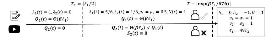
Figure 2: An example where BACID.UCB fails to correctly classify video (type-$2$) posts. Humans never review a video because the corresponding queue length is much smaller than that of texts.

BACID.UCB incurs linear regret in the above example as its decisions are inherently myopic to current rounds and disregard the importance of labels towards classification decisions in future rounds. Broadly speaking, optimism-only heuristics focus on the most optimistic estimate on the contribution of each action (in our setting, the admission decision) subject to a confidence interval and then select the action that maximizes this optimistic contribution in the current round. In our example, if we can only admit one type, the text posts have larger idiosyncrasy loss due to their lifetime and thus the benefit of admitting a text post outweighs even the most optimistic estimate on the idiosyncrasy loss of video posts in the current round. This mimics the admission rule of BACID which operates with known parameters and would never review a video post. Although always prioritizing text posts is myopically beneficial in the current round, this means that we collect no new video data, thus harming our classification performance in the long run.

4.2 Label-Driven Admission and Forced Scheduling for Classification

The inefficiency of BACID.UCB suggests the need to complement the myopic nature of optimism-only approaches by a forward-looking exploration that enhances classification decisions. Our algorithm, Optimistic and Label-driven Admission for Balanced Classification, Idiosynrasy and Delay or OLBACID in short (Algorithm 2)) incorporates this forward-looking exploration and evades the shortcomings of optimism-only approaches. When a new post of type $k$ arrives, we classify it as harmful/remove it ($Y_{k}(t)=0$) if and only if the empirical average cost $\hat{h}_{k}(t)$ is positive. Unlike BACID which assumes knowledge of $h_{k}$, when $\underline{h}_{k}(t)<0<\bar{h}_{k}(t)$, we cannot confidently infer the sign of $h_{k}$ from the sign of $\hat{h}_{k}(t)$.

To enhance future classification decisions on those posts, we complement the optimism-based admission (Line 2) with a label-driven admission (Line 2). Specifically, we maintain a new label-driven queue $\mathcal{Q}^{\textsc{ld}}(t)$ and add the post to that queue ($E_{k}(t)=1$) if the queue is empty and there is high uncertainty on the sign of $\hat{h}_{k}(t)$, i.e., $\underline{h}_{k}(t)\leq-\gamma$ and $\gamma\leq\bar{h}_{k}(t)$ where $\gamma$ is a parameter that avoids wasting reviewing capacity on posts that are already well classified. If the post is admitted into the review queue by the optimism-based admission ($E_{k}(t)=0$, $\beta\bar{r}_{k}(t)\ell_{k}\geq Q_{k}(t)$), we denote $A_{k}(t)=1$. We stress that $Q_{k}(t)$ includes only posts in the review queue $\mathcal{Q}(t)$ and not in $\mathcal{Q}^{\mathcal{\textsc{LD}}}(t)$.

We use forced scheduling to prioritize reviews for the label-driven queue. If $\mathcal{Q}^{\mathcal{\textsc{LD}}}(t)$ is not empty, we review a post from $\mathcal{Q}^{\mathcal{\textsc{LD}}}(t)$. Otherwise, we follow the MaxWeight scheduling (as in BACID): select a type $k^{\prime}$ that maximizes $\mu_{k^{\prime}}Q_{k^{\prime}}(t)$ and review the earliest waiting post in the review queue $\mathcal{Q}(t)$ that has type $k^{\prime}$. We let $\psi_{k^{\prime}}(t)=1$ if a type-$k^{\prime}$ post in $\mathcal{Q}(t)$ is scheduled to review in period $t$.

Data: $(\ell_{k},\mu_{k},\sigma_{k}\}_{k\in\mathcal{K}},H$

1 $\gamma=\beta\leftarrow 1/\sqrt{K\ell_{\max}}$ // Label-driven & Optimistic Admission Parameters

2 for $t=1$ to $T$ do

3       Observe a new post $j(t)=j$ of type $k(j)=k$; if no new post, set $j(t)=\perp$

4       if $\hat{h}_{k}(t)>0$ then $Y_{k}(t)\leftarrow 0$ else $Y_{k}(t)\leftarrow 1$ // Empirical Classification

       /* Label-Driven and Optimistic Admission */

5       $\bar{r}_{k}(t)=\max_{h\in[\underline{h}_{k}(t),\bar{h}_{k}(t)]}r_{k}(h)$ where $\underline{h}_{k}(t),\bar{h}_{k}(t)$ are given by (9)

6       if $\underline{h}_{k}(t)<-\gamma<\gamma<\bar{h}_{k}(t)$ and $|\mathcal{Q}^{\mathcal{\textsc{LD}}}(t)|=0$ then  $E_{k}(t)\leftarrow 1$ else $E_{k}(t)=0$

7      

8      if $E_{k}(t)=0$ and $\beta\cdot\bar{r}_{k}(t)\cdot\ell_{k}\geq Q_{k}(t)$ then  $A_{k}(t)=1$ else $A_{k}(t)=0$

       /* Forced Scheduling and MaxWeight Scheduling */

9      

10      if $\mathcal{Q}^{\mathcal{\textsc{LD}}}(t)\neq\emptyset$ then $M(t)\leftarrow$ the post in $\mathcal{Q}^{\mathcal{\textsc{LD}}}(t)$

11       else  $k^{\prime}\leftarrow\arg\max_{k^{\prime}\in\mathcal{K}}\mu_{k^{\prime}}\cdot Q_{k^{\prime}}(t)$, $M(t)\leftarrow\text{first post in }\mathcal{Q}_{k^{\prime}}(t)\text{ if any}$

12       if the review finishes (with probability $N(t)\cdot\mu_{k(M(t))}$) then  $\mathcal{S}(t)=M(t)$ else $\mathcal{S}(t)=\perp$

13      

Algorithm 2 Optimistic and Label-driven BACID (OLBACID)

Our main result (Theorem 3) is that, setting $\beta=\gamma=1/\sqrt{K\ell_{\max}}$, OLBACID achieves an average regret of $\tilde{O}(\sqrt{\ell_{\max}}+\ell_{\max}/\sqrt{T}+\ell_{\max}^{1.5}/T)$ when there is a large margin $\eta$ and small number of types $K$. In particular, the guarantee matches the lower bound $O(\sqrt{\ell_{\max}})$ when $T\geq\ell_{\max}$. Even if there is no margin (so classification is difficult), OLBACID still obtains an average regret of $\tilde{O}(\sqrt{\ell_{\max}}+\ell_{\max}/\sqrt{T}+\ell_{max}^{2}/T)$, which matches the lower bound when $T\geq\ell_{\max}^{1.5}$.

Theorem 3.

For a window size $w$, the average regret of OLBACID is upper bounded by

$$\textsc{Reg}^{\textsc{OLBACID}}(w,T)\lesssim w\sqrt{K\ell_{\max}}+K\ell_{\max}\sqrt{\frac{1}{T}}+\frac{\sqrt{K}\ell_{\max}^{1.5}}{T}+\min\left(\frac{K\ell_{\max}}{\eta^{2}T},\frac{K^{2}\ell_{\max}^{2}}{T}\right).$$

To prove Theorem 3, we need a loss decomposition of $\mathcal{L}^{\textsc{OLBACID}}(T)$ as in (1) that also captures the possible incorrect classification decisions. The incurred loss per period is thus given by $r_{k}^{O}\cdot(1-Y_{k}(t))+r_{k}^{R}\cdot Y_{k}(t)$ instead of $r_{k}=\min(r_{k}^{O},r_{k}^{R})$. Following the same analysis of (1), we have

$$\mathbb{E}\left[\mathcal{L}^{\textsc{OLBACID}}(T)\right] =\mathbb{E}\left[\sum_{t=1}^{T}\sum_{k\in\mathcal{K}}\left(r_{k}^{O}\cdot Y_{k}(t)+r_{k}^{R}\cdot(1-Y_{k}(t))\right)\ell_{k}(\Lambda_{k}(t)-A_{k}(t)-E_{k}(t))\right]$$

$$+\mathbb{E}\left[\sum_{t=1}^{T}(A_{k(j(t))}(t)+E_{k(j(t))}(t))\left(r_{k}^{O}\cdot Y_{k}(t)+r_{k}^{R}\cdot(1-Y_{k}(t))\right)\min\left(D(j(t)),\ell_{k(j)}\right)\right].$$

Using $r_{k}^{O},r_{k}^{R}\leq r_{\max}$ and applying Little’s Law, we upper bound $\mathbb{E}\left[\mathcal{L}^{\textsc{OLBACID}}(T)\right]$ by

$$\hskip 7.22743pt\underbrace{\mathbb{E}\left[\sum_{t=1}^{T}\sum_{k\in\mathcal{K}}(Y_{k}(t)(r_{k}^{O}-r_{k}^{R})^{+}+(1-Y_{k}(t))(r_{k}^{R}-r_{k}^{O})^{+})\ell_{k}(\Lambda_{k}(t)-A_{k}(t)-E_{k}(t))\right]}_{\text{Classification Loss}}$$

$$+\underbrace{\mathbb{E}\left[\sum_{t=1}^{T}\sum_{k\in\mathcal{K}}r_{k}\ell_{k}(\Lambda_{k}(t)-A_{k}(t)-E_{k}(t))\right]}_{\text{Idiosyncrasy Loss}}+\underbrace{r_{\max}\mathbb{E}\left[\sum_{t=1}^{T}\left(\sum_{k\in\mathcal{K}}Q_{k}(t)+|\mathcal{Q}^{\mathcal{\textsc{LD}}}(t)|\right)\right]}_{\text{Relaxed Delay Loss}}.$$ (10)

Comparing (10) with (2), there is a new term on classification loss, which captures the loss when the classification $Y_{k}(t)$ is incorrect. We adjust the other terms to capture label-driven admission.

To bound those three losses, we define the maximum per-period views and cost standard deviation as $v_{\max}=\max(1,\max_{k}v_{k})$, $\sigma_{\max}=\max\left(1,\max_{k\in\mathcal{K}}\sigma_{k}\right)$ respectively, and the minimum per-period review rate as $\hat{\mu}_{\min}=\min_{t\in[T],k\in\mathcal{K}}N(t)\mu_{k}$. To account for uncertainty, we take $r_{\max}=v_{\max}(H+\sigma_{\max})\geq 1$; this is an upper bound on $r_{k}^{O}(\cdot),r_{k}^{R}(\cdot)$ by their definition Eq. (3). We focus on $T\geq 3$ and $K\leq\ell_{\max}$ (the bound in Theorem 3 becomes trivial if $K>\ell_{\max}$). Our bounds (Lemmas 4.1, 4.2 and 4.3) hold for general $\beta,\gamma$, and are proven in Sections 4.3, 4.4 and 4.5 respectively. The lemmas are defined for $T\geq 3$ and $K\leq\ell_{\max}$ (the bound in Theorem 3 becomes trivial otherwise). The proof of Theorem 3 (provided in Appendix C.4) directly combines the lemmas.

Lemma 4.1.

For any $\beta,\gamma\in(1/\ell_{\max},1]$, the Relaxed Delay Loss of OLBACID is at most

$$2K\beta r^{2}_{\max}\ell_{\max}T+\frac{33r_{\max}K\sigma^{2}_{\max}\ln T}{\hat{\mu}_{\min}\max(\eta,\gamma)^{2}}.$$

Lemma 4.2.

For any $\beta,\gamma\in(1/\ell_{\max},1]$, the Classification Loss of OLBACID is at most

$$4\ell_{\max}\left(v_{\max}\gamma T+Kr_{\max}\right)+\frac{33r_{\max}\ell_{\max}K\sigma_{\max}^{2}\ln T}{\hat{\mu}_{\min}\max(\eta,\gamma)^{2}}.$$

Lemma 4.3.

For any $\beta,\gamma\in(1/\ell_{\max},1]$, the Idiosyncrasy Loss of OLBACID is at most

$$\mathcal{L}^{\star}(w,T)+\frac{wT}{\beta}+\frac{66r_{\max}\ell_{\max}K\sigma^{2}_{\max}\ln T}{\max(\eta,\gamma)^{2}\hat{\mu}_{\min}}+18Kr_{\max}\ell_{\max}\left(\sqrt{T\ln T}+\beta r_{\max}\ell_{\max}\right)$$

4.3 Bounding Forced Scheduling and Relaxed Delay Loss (Lemma 4.1)

A key ingredient in the proof of all of Lemmas 4.1, 4.2, and 4.3 is to provide an upper bound on the number of periods that the label-driven queue is non-empty. Given that $\mathcal{Q}^{\mathcal{\textsc{LD}}}(t)$ has at most one post at any period $t$, letting $Q^{\mathcal{\textsc{LD}}}(t)=|\mathcal{Q}^{\mathcal{\textsc{LD}}}(t)|$, this is equal to $\mathbb{E}\left[\sum_{t=1}^{T}Q^{\mathcal{\textsc{LD}}}(t)\right]$. This quantity allows to bound 1) the number of posts which we do not admit into the label-driven queue despite not being able to confidently estimate the sign of their expected cost; 2) the delay loss; 3) the number of periods that we do not follow MaxWeight scheduling.

Our first lemma connects $\mathbb{E}\left[\sum_{t=1}^{T}Q^{\mathcal{\textsc{LD}}}(t)\right]$ to the number of posts admitted to the label-driven queue $\mathcal{Q}^{\textsc{ld}}(t)$. The proof (Appendix C.3) relies on only admitting posts when $\mathcal{Q}^{\textsc{ld}}(t)$ is empty.

Lemma 4.4.

The label-driven queue admits at most $\mathbb{E}\left[\sum_{t=1}^{T}Q^{\mathcal{\textsc{LD}}}(t)\right]\leq\frac{\mathbb{E}\left[\sum_{t=1}^{T}\sum_{k\in\mathcal{K}}E_{k}(t)\right]}{\hat{\mu}_{\min}}$posts.

Our second lemma applies concentration bounds (Appendix C.5) to show that the event $\mathcal{E}_{k,t}=\{h_{k}\in[\underline{h}_{k}(t),\bar{h}_{k}(t)]\}$ (expected cost lies in confidence interval) holds with high probability.

Lemma 4.5.

For any $k,t$, the expected cost lies in $[\underline{h}_{k}(t),\bar{h}_{k}(t)]$ with probability $\mathbb{P}\{\mathcal{E}_{k,t}\}\geq 1-2t^{-3}$.

Our next lemma (proof in Appendix C.6) bounds $\mathbb{E}\left[\sum_{t=1}^{T}\sum_{k\in\mathcal{K}}E_{k}(t)\right]$ via considering the type-$k$ confidence interval when the last type-$k$ post is admitted to the label-driven queue $\mathcal{Q}^{\textsc{ld}}$.

Lemma 4.6.

The label-driven queue admits at most $\mathbb{E}\left[\sum_{t=1}^{T}\sum_{k\in\mathcal{K}}E_{k}(t)\right]\leq\frac{33K\sigma^{2}_{\max}\ln T}{\max(\eta,\gamma)^{2}}$ posts.

Our final lemma bounds the length of the review queue (similar to Lemma 3.2).

Lemma 4.7.

For any $k,t$, the optimistic queue has at most $Q_{k}(t)\leq 2\beta r_{\max}\ell_{\max}$ posts.

Proof.

We admit a type-$k$ post into $\mathcal{Q}$ only if $\beta\bar{r}_{k}(t)\ell_{k}\leq Q_{k}(t)$ and $\bar{r}_{k}(t)\leq r_{\max}$. As in the proof of Lemma 3.2, the queue length is bounded by $Q_{k}(t)\leq\beta r_{\max}\ell_{\max}+1\leq 2\beta r_{\max}\ell_{\max}$. ∎

Proof of Lemma 4.1.

By definition, the Relaxed Delay Loss is upper bounded by

$$r_{\max}\mathbb{E}\left[\sum_{t=1}^{T}\left(\sum_{k\in\mathcal{K}}Q_{k}(t)+|\mathcal{Q}^{\mathcal{\textsc{LD}}}(t)|\right)\right]\leq 2r_{\max}K\beta r_{\max}\ell_{\max}T+\frac{33r_{\max}K\sigma^{2}_{\max}\ln T}{\max(\eta,\gamma)^{2}\hat{\mu}_{\min}},$$

where we use Lemma 4.7 for the first term and Lemmas 4.4 and 4.6 for the second term. ∎

4.4 Bounding the Classification Loss (Lemma 4.2)

Our first lemma (proof in Appendix C.7) shows a Lipschitz property for functions $r_{k}^{O}(\cdot),r_{k}^{R}(\cdot),r_{k}(\cdot)$.

Lemma 4.8.

For any type $k$, functions $r_{k}^{O}(h),r_{k}^{R}(h)$ and $r_{k}(h)$ are $1.5v_{k}$-Lipschitz continuous.

Our next lemma (proof in Appendix C.8) uses this property to establish a bound on the type-$k$ period-$t$ classification loss $Z_{k}(t)=(Y_{k}(t)(r_{k}^{O}-r_{k}^{R})^{+}+(1-Y_{k}(t))(r_{k}^{R}-r_{k}^{O})^{+})\ell_{k}(\Lambda_{k}(t)-A_{k}(t)-E_{k}(t))$.

Lemma 4.9.

For any type $k$ and period $t$, $Z_{k}(t)\mathbbm{1}\left(\mathcal{E}_{k,t}\right)\leq\left(3v_{\max}\gamma\ell_{\max}+r_{\max}\ell_{\max}Q^{\mathcal{\textsc{LD}}}(t)\right)\Lambda_{k}(t).$

Proof of Lemma 4.2.

By definition, the total classification loss is $\mathbb{E}\left[\sum_{t=1}^{T}\sum_{k\in\mathcal{K}}Z_{k}(t)\right]$. As a result,

$$\mathbb{E}\left[\sum_{t=1}^{T}\sum_{k\in\mathcal{K}}Z_{k}(t)\right] \leq\mathbb{E}\left[\sum_{t=1}^{T}\sum_{k\in\mathcal{K}}Z_{k}(t)\mathbbm{1}\left(\mathcal{E}_{k,t}\right)\right]+r_{\max}\ell_{\max}\sum_{t=1}^{T}\sum_{k\in\mathcal{K}}\mathbb{P}\{\mathcal{E}_{k,t}^{c}\} Z_{k}(t)\leq r_{\max}\ell_{\max}$$ ()

$$\leq\mathbb{E}\left[\sum_{t=1}^{T}\sum_{k\in\mathcal{K}}Z_{k}(t)\mathbbm{1}\left(\mathcal{E}_{k,t}\right)\right]+Kr_{\max}\ell_{\max}\sum_{t=1}^{T}\frac{2}{t^{3}}$$ (By Lemma 4.5)

$$\leq\mathbb{E}\left[\sum_{t=1}^{T}\left(3v_{\max}\gamma\ell_{\max}+r_{\max}\ell_{\max}Q^{\mathcal{\textsc{LD}}}(t)\right)\right]+4Kr_{\max}\ell_{\max}$$ (By Lemma 4.9)

$$\leq 3v_{\max}\gamma\ell_{\max}T+\frac{33r_{\max}\ell_{\max}K\sigma^{2}_{\max}\ln T}{\max(\eta,\gamma)^{2}\hat{\mu}_{\min}}+4Kr_{\max}\ell_{\max}.$$ (By Lemmas 4.4, 4.6)

∎

4.5 Bounding the Idiosyncrasy Loss (Lemma 4.3)

We follow a similar strategy as in the proof of Lemma 3.1, but we encounter three new challenges due to the algorithmic differences between BACID and OLBACID.

Our first challenge arises because of the additional label-driven admission. Without the label-driven admission, we would admit a type-$k$ post to the review queue $\mathcal{Q}(t)$ in period $t$ if its (optimistic) idiosyncrasy loss outweighs the delay loss, i.e., $\bar{A}_{k}(t)=\Lambda_{k}(t)\mathbbm{1}\left(\beta\bar{r}_{k}(t)\ell_{k}\geq Q_{k}(t)\right)$ is equal to one. However, we now only admit such a post to $\mathcal{Q}(t)$ if it is not admitted to the label-driven queue $\mathcal{Q}^{\mathcal{\textsc{LD}}}(t)$, i.e., the real admission decision is $A_{k}(t)=\bar{A}_{k}(t)(1-E_{k}(t))$. The following Lyapunov function defined based on only the length of $\mathcal{Q}(t)$ accounts for this difference and offers an analogue of Lemma 3.3, which we prove in Appendix C.9.

$$L(t)=\beta\sum_{t^{\prime}=1}^{t-1}\sum_{k\in\mathcal{K}}r_{k}\ell_{k}(\Lambda_{k}(t^{\prime})-A_{k}(t^{\prime})-E_{k}(t^{\prime}))+\frac{1}{2}\sum_{k\in\mathcal{K}}Q_{k}^{2}(t),$$

Lemma 4.10.

The expected Lagrangian of OLBACID upper bounds the idiosyncrasy loss by:

$$\beta\mathbb{E}\left[\sum_{t=1}^{T}\sum_{k\in\mathcal{K}}r_{k}\ell_{k}(\Lambda_{k}(t)-A_{k}(t)-E_{k}(t))\right]\leq\mathbb{E}\left[L(T+1)-L(1)\right]\leq T+\sum_{t=1}^{T}\mathbb{E}\left[f_{t}(\boldsymbol{\bar{A}}(t),\boldsymbol{\psi}(t),\boldsymbol{Q}(t))\right].$$

We next bound the right hand side of Lemma 4.10. By Lemma 3.4, we know how to bound this quantity when admission and scheduling decisions are made according to BACID, i.e., $A_{k}^{\textsc{BACID}}(t)=\mathbbm{1}\left(\beta r_{k}\ell_{k}\geq Q_{k}(t)\right)\Lambda_{k}(t)$ and $\psi_{k}^{\textsc{BACID}}(t)=\mathbbm{1}\left(k=\arg\max_{k^{\prime}\in\mathcal{K}}\mu_{k}Q_{k}(t)\right)$. To bound the Lagrangian under OLBACID, we connect it to its analogue under BACID via the regret in Lagrangian:

$$\textsc{RegL}(T) =\mathbb{E}\left[\sum_{t=1}^{T}f_{t}(\boldsymbol{\bar{A}}(t),\boldsymbol{\psi}(t),\boldsymbol{Q}(t))-f_{t}(\boldsymbol{A}^{\textsc{BACID}}(t),\boldsymbol{\psi}^{\textsc{BACID}}(t),\boldsymbol{Q}(t))\right]$$

$$=\underbrace{\mathbb{E}\left[\sum_{t=1}^{T}\sum_{k\in\mathcal{K}}(A_{k}^{\textsc{BACID}}(t)-\bar{A}_{k}(t))(\beta r_{k}\ell_{k}-Q_{k}(t))\right]}_{\textsc{RegA}(T)}+\underbrace{\mathbb{E}\left[\sum_{t=1}^{T}\sum_{k\in\mathcal{K}}(\psi_{k}^{\textsc{BACID}}(t)-\psi_{k}(t))Q_{k}(t)\mu_{k}N(t)\right]}_{\textsc{RegS}(T)}$$

Our second challenge is to upper bound the regret in admission $\textsc{RegA}(T)$. Unlike BACID which admits based on the ground-truth per-period idiosyncrasy loss $r_{k}$, OLBACID uses the optimistic estimation $\bar{r}_{k}(t)$. Unlike works in bandits with knapsacks, the following lemma also needs to account for the endogenous queueing delay in label acquisition (proof in Appendix C.10).

Lemma 4.11.

The regret in admission is $\textsc{RegA}(T)\leq 12K\beta^{2}r^{2}_{\max}\ell^{2}_{\max}+6K\beta r_{\max}\ell_{\max}\sqrt{8T\ln T}.$

Our third challenge is to bound the regret in scheduling $\textsc{RegS}(T)$. Unlike BACID which schedules based on MaxWeight, OLBACID prioritizes posts in the $\mathcal{Q}^{\mathcal{\textsc{LD}}}(t)$. The effect of those deviations is bounded in the next lemma (proof in Appendix C.11), using Lemmas 4.4 and 4.6.

Lemma 4.12.

The regret in scheduling is $\textsc{RegS}(T)\leq\frac{66\beta r_{\max}\ell_{\max}K\sigma^{2}_{\max}\ln T}{\max(\eta,\gamma)^{2}\hat{\mu}_{\min}}$.

Proof of Lemma 4.3.

By Lemma 4.10, the idiosyncrasy loss is upper bounded by

$$\beta\mathbb{E}\left[\sum_{t=1}^{T}\sum_{k\in\mathcal{K}}r_{k}\ell_{k}(\Lambda_{k}(t)-A_{k}(t)-E_{k}(t))\right] \leq T+\sum_{t=1}^{T}\mathbb{E}\left[f_{t}(\boldsymbol{\bar{A}}(t),\boldsymbol{\psi}(t),\boldsymbol{Q}(t))\right]$$

$$=T+\sum_{t=1}^{T}\mathbb{E}\left[f_{t}(\boldsymbol{A}^{\textsc{BACID}}(t),\boldsymbol{\psi}^{\textsc{BACID}}(t),\boldsymbol{Q}(t))\right]+\textsc{RegL}(T)$$

$$\leq wT+\beta\mathcal{L}^{\star}(w,T)+\textsc{RegA}(T)+\textsc{RegS}(T)$$ (By Lemma 3.4)

$$\leq wT+\beta\mathcal{L}^{\star}(w,T)+12K\beta^{2}r^{2}_{\max}\ell^{2}_{\max}+6K\beta r_{\max}\ell_{\max}\sqrt{8T\ln T}+\frac{66\beta r_{\max}\ell_{\max}K\sigma^{2}_{\max}\ln T}{\max(\eta,\gamma)^{2}\hat{\mu}_{\min}}$$ (By Lemmas 4.11 and 4.12)

$$\leq wT+\beta\mathcal{L}^{\star}(w,T)+\frac{66\beta r_{\max}\ell_{\max}K\sigma^{2}_{\max}\ln T}{\max(\eta,\gamma)^{2}\hat{\mu}_{\min}}+18K\beta r_{\max}\ell_{\max}\left(\sqrt{T\ln T}+\beta r_{\max}\ell_{\max}\right).$$

Dividing both sides of the inequality by $\beta$ gives the desired result. ∎

5 OLBACID with Type Aggregation and Contextual Learning

In this section, we design an algorithm whose performance does not deteriorate with the number of types $K$. We adopt a linear contextual structure assumption that is common in the bandit literature [LCLS10, CLRS11, APS11], and in online content moderation practice [ABB⁺22]. Each post comes with a $d$-dimensional feature vector $\boldsymbol{\phi}_{k}\in\mathbb{R}^{d}$ associated with its type $k$ and its expected cost satisfies a linear model $h_{k}=\boldsymbol{\phi}_{k}^{\intercal}\boldsymbol{\theta}^{\star}$ for a fixed unknown vector $\boldsymbol{\theta}^{\star}$.

We incorporate the contextual information in our confidence intervals around $h_{k}$ by classical bandit techniques [APS11]; we provide a more detailed comparison in Appendix D.1. We construct a confidence set $\mathcal{C}_{t}$ for $\boldsymbol{\theta}^{\star}$ based on the collected data set $\mathcal{D}(t)$. Recalling that $\mathcal{S}(\tau)$ is the reviewed post for period $\tau$ (or $\perp$ when no post is reviewed), the dataset in period $t$ is $\{(\boldsymbol{X}_{\tau},Z_{\tau})\}_{\tau\leq t}$ with $\boldsymbol{X}_{\tau}=\boldsymbol{\phi}_{k(\mathcal{S}(\tau))}$ and $Z_{\tau}=c_{\mathcal{S}(\tau)}$. We use the ridge estimator with regularization parameter $\kappa$, i.e,

$$\hat{\boldsymbol{\theta}}(t)=\bar{\boldsymbol{V}}_{t}^{-1}[\boldsymbol{X}_{1},\ldots,\boldsymbol{X}_{t}][Z_{1},\ldots,Z_{t}]^{\intercal}\quad\text{where}\quad\bar{\boldsymbol{V}}_{t}=\kappa\boldsymbol{I}+\sum_{\tau\leq t}\boldsymbol{X}_{\tau}\boldsymbol{X}_{\tau}^{\intercal}\quad\text{and}\quad\hat{\boldsymbol{\theta}}(0)=\boldsymbol{0}.$$ (11)

Recalling that $\sigma_{\max}=\max_{k\in\mathcal{K}}\sigma_{k}$ is the maximum idiosyncrasy variance and $U$ upper bounds the Euclidean norm of $\boldsymbol{\theta}^{\star}$ and any feature $\boldsymbol{\phi}_{k}$, we define the confidence set with a confidence level $\delta$ by

$$\mathcal{C}_{t}\coloneqq\left\{\boldsymbol{\theta}\in\mathbb{R}^{d}\colon\|\hat{\boldsymbol{\theta}}(t)-\boldsymbol{\theta}\|_{\bar{\boldsymbol{V}}_{t}}\leq B_{\delta}(t)\right\}\quad\text{where }B_{\delta}(t)\coloneqq\sigma_{\max}\sqrt{d\ln\left(\frac{1+tU^{2}/\kappa}{\delta}\right)}+\sqrt{\kappa}U.$$ (12)

Using confidence set $\mathcal{C}_{t-1}$, we can modify our confidence intervals from (9) for period $t$ as follows:

$$\underline{h}_{k}(t)=\max\left(-H,\min_{\boldsymbol{\theta}\in\mathcal{C}_{t-1}}\boldsymbol{\phi}_{k}^{\intercal}\boldsymbol{\theta}\right),\quad\bar{h}_{k}(t)=\min\left(H,\max_{\boldsymbol{\theta}\in\mathcal{C}_{t-1}}\boldsymbol{\phi}_{k}^{\intercal}\boldsymbol{\theta}\right),\quad\bar{r}_{k}(t)=\max_{h\in[\underline{h}_{k}(t),\bar{h}_{k}(t)]}r_{k}(h).$$ (13)

5.1 Type Aggregation for Better Idiosyncrasy and Delay Tradeoff

An additional challenge when the number of types $K$ is large (that arises even without learning) is the difficulty to estimate delay loss; this is crucial in the design of BACID which admits a post if and only if its idiosyncrasy loss is above an estimated delay loss. BACID estimates the delay loss of a post based on the number of same-type waiting posts. With a large $K$, this approach underestimates the real delay loss, leading to overly admitting posts into the review system. An alternative delay estimator uses the total number of waiting posts $|\mathcal{Q}(t)|$. This ignores the heterogeneous delay loss of admitting different types. In particular, our scheduling algorithm prioritizes posts with less review workload (higher $\mu_{k}$) to effectively manage the limited capacity. A post with a higher service rate thus has smaller delay loss and neglecting this heterogeneity results in overestimating its delay loss.

To address this challenge, we create an estimator for the delay loss that lies in the middle ground of the aforementioned estimators. In particular, we map each type $k$ to a group $g(k)$ based on its service rates; we denote this partition by $\mathcal{K}_{\mathcal{G}}=\{\mathcal{K}_{g}\}_{g\in\mathcal{G}}$ where $\mathcal{G}$ is the set of groups, $G=|\mathcal{G}|$ is its cardinality, and $\mathcal{K}_{g}$ is the set of types in group $g\in\mathcal{G}$. For a group $g$, we define its proxy service rate $\tilde{\mu}_{g}=\min_{k\in\mathcal{K}_{g}}\mu_{k}$ as the minimum service rate across types in this group. For a new post of type $k$, we estimate its delay loss by the number of posts of types in $\mathcal{K}_{g(k)}$ waiting in the review queue. This estimator is efficient if the number of groups is small, and service rates of types in a group are close to each other. Specifically, letting $N_{\max}=\max_{t}N(t)$ be the maximum number of reviewers, we define the aggregation gap $\Delta(\mathcal{K}_{\mathcal{G}})=\max_{g\in\mathcal{G}}\max_{k\in\mathcal{K}_{g}}N_{\max}(\mu_{g}-\tilde{\mu}_{g})$ of a group partition $\mathcal{K}_{\mathcal{G}}$ as the maximum within-group service rate difference (scaled by reviewing capacity).

5.2 Algorithm, Theorem and Proof Sketch

Our algorithm, Contextual OLBACID (Algorithm 3), or COLBACID in short, works as follows. In period $t$, we first compute a ridge estimator $\hat{\boldsymbol{\theta}}(t)$ of $\boldsymbol{\theta}^{\star}$ by (11). The algorithm then classifies a new type-$k$ post as harmful ($Y_{k}(t)=0$) if its empirical average cost, $\boldsymbol{\phi}_{k}^{\intercal}\hat{\boldsymbol{\theta}}(t)$, is positive. We follow the same label-driven admission with OLBACID in Line 3 but we set the confidence interval on $h_{k}$ by (13) using the confidence set $\mathcal{C}_{t}$ from (12). The optimistic admission rule (Line 3) similarly finds an optimistic per-period idiosyncrasy loss $\bar{r}_{k}(t)$ but estimates the delay loss by type-aggregated queue lengths. Specifically, letting $\tilde{\mathcal{Q}}_{g}(t)=\{j\in\mathcal{Q}(t)\colon g(k(j))=g\}$ be the set of waiting posts whose types belong to group $g$ and $\tilde{Q}_{g}(t)=|\tilde{\mathcal{Q}}_{g}(t)|$, we admit a type-$k$ post if and only if its (optimistic) idiosyncrasy loss is higher than the estimated delay loss, i.e., $\beta\bar{r}_{k(t)}(t)\ell_{k}\geq\tilde{Q}_{g(k(t))}(t)$. We still prioritize the label-driven queue for scheduling. If there is no post in the label-driven queue, we use a type-aggregated MaxWeight scheduling: we first pick a group $g$ maximizing $\tilde{\mu}_{g}\tilde{Q}_{g}(t)$, and then pick the earliest admitted post in the review queue $\mathcal{Q}(t)$ whose type is of group $g$ to review.

Data: $(\ell_{k},\mu_{k},\sigma_{k}\}_{k\in\mathcal{K}}$, upper bounds $U,H$, and group partition $\mathcal{K}_{\mathcal{G}}$

1 $\beta,\gamma\leftarrow 1/\sqrt{G\ell_{\max}},~{}\delta\leftarrow\min(\gamma,1/T),~{}\kappa\leftarrow\max(1,U^{2})$

2 for $t=1$ to $T$ do

3       Observe a new post $j(t)=j$ of type $k(j)=k$; if no new post, set $j(t)=\perp$

4       Compute ridge estimator $\hat{\boldsymbol{\theta}}(t)$ by (11)

5       if $\boldsymbol{\phi}_{k}^{\intercal}\hat{\boldsymbol{\theta}}(t)>0$ then $Y_{k}(t)\leftarrow 0$ else $Y_{k}(t)\leftarrow 1$ // Empirical Classification

       /* Label-Driven and Optimistic Admission */

6       $\bar{r}_{k}(t)=\max_{h\in[\underline{h}_{k}(t),\bar{h}_{k}(t)]}r_{k}(h)$ where $\underline{h}_{k}(t),\bar{h}_{k}(t)$ are given by (13)

7       if $\underline{h}_{k}(t)<-\gamma<\gamma<\bar{h}_{k}(t)$ and $|\mathcal{Q}^{\mathcal{\textsc{LD}}}(t)|=0$ then  $E_{k}(t)\leftarrow 1$ else $E_{k}(t)=0$

8       if $E_{k}(t)=0$ and $\beta\cdot\bar{r}_{k}(t)\cdot\ell_{k}\geq\tilde{Q}_{g(k)}(t)$ then  $A_{k}(t)=1$ else $A_{k}(t)=0$ // Admission

       /* Forced Scheduling and Type-Aggregated MaxWeight Scheduling */

9       if $\mathcal{Q}^{\mathcal{\textsc{LD}}}(t)\neq\emptyset$ then $M(t)\leftarrow$ the post in $\mathcal{Q}^{\mathcal{\textsc{LD}}}(t)$

10       else  $g\leftarrow\arg\max_{g\in\mathcal{G}}\tilde{\mu}_{g}\cdot\tilde{Q}_{g}(t)$, $M(t)\leftarrow\text{first post in }\tilde{\mathcal{Q}}_{g}(t)\text{ if any}$

11       if the review finishes (with probability $N(t)\cdot\mu_{k(M(t))}$) then  $\mathcal{S}(t)=M(t)$ else $\mathcal{S}(t)=\perp$

12      

Algorithm 3 Contextual OLBACID (COLBACID)

For ease of exposition, we follow the $\lesssim$ notation to include only super-logarithmic dependence on the number of groups $G$, feature dimension $d$, maximum lifetime $\ell_{\max}$, the margin $\eta$, window size $w$, the time horizon $T$, and the aggregation gap $\Delta(\mathcal{K}_{\mathcal{G}})$. Our main result is as follows.

Theorem 4.

For a window size $w$, the average regret of COLBACID is upper bounded by

$$\textsc{Reg}^{\textsc{COLBACID}}(w,T)\lesssim w\sqrt{G\ell_{\max}}+\ell_{\max}\left(\Delta(\mathcal{K}_{\mathcal{G}})+d\sqrt{\frac{G}{T}}+\frac{\sqrt{G}\ell_{\max}^{0.5}d^{1.5}}{T}+\frac{d^{2.5}}{T}\min\left(\frac{1}{\eta^{2}},G\ell_{\max}\right)\right).$$

Note that, if, for all groups $g\in\mathcal{G}$, all types $k\in\mathcal{K}_{g}$ have the same service rate, then $\Delta(\mathcal{K}_{\mathcal{G}})=0$, but the regret still depends on $G$ which is large if there are many types with unequal service rates.

To provide a worst-case guarantee, we select a fixed aggregation gap $0<\zeta\leq 1$ and create a partition $\mathcal{K}_{\mathcal{G}}^{\zeta}$ that segments types based on the their maximum scaled service rate $N_{\max}\mu_{k}$ into intervals $(0,\zeta],(\zeta,2\zeta],\ldots,(\lfloor\frac{1}{\zeta}\rfloor\zeta,1]$. The number of groups is at most $G\leq\frac{1}{\zeta}+1\leq\frac{2}{\zeta}$ and the aggregation gap $\Delta(\mathcal{K}_{\mathcal{G}}^{\zeta})$ is at most $\zeta$. Optimizing the bound in Theorem 4 for the term $w\sqrt{G\ell_{\max}}+\Delta(\mathcal{K}_{\mathcal{G}})\ell_{\max}$, and setting $\zeta=\ell_{\max}^{-1/3}$ we obtained the following result.

Corollary 1.

For a window size $w$, COLBACID with group partition $\mathcal{K}_{\mathcal{G}}^{\zeta}$ satisfies:

$$\textsc{Reg}^{\textsc{COLBACID}}(w,T)\lesssim w\ell_{\max}^{2/3}+\ell_{\max}\left(\frac{\ell_{\max}^{1/6}d}{\sqrt{T}}+\frac{\ell_{\max}^{2/3}d^{1.5}}{T}+\frac{d^{2.5}}{T}\min\left(\frac{1}{\eta^{2}},\ell_{\max}^{4/3}\right)\right).$$

The proof of Theorem 4 (Appendix D.2) bounds the losses in the same decomposition as in (10),

$$\hskip 7.22743pt\underbrace{\mathbb{E}\left[\sum_{t=1}^{T}\sum_{k\in\mathcal{K}}(Y_{k}(t)(r_{k}^{O}-r_{k}^{R})^{+}+(1-Y_{k}(t))(r_{k}^{R}-r_{k}^{O})^{+})\ell_{k}(\Lambda_{k}(t)-A_{k}(t)-E_{k}(t))\right]}_{\text{Classification Loss}}$$

$$+\underbrace{\mathbb{E}\left[\sum_{t=1}^{T}\sum_{k\in\mathcal{K}}r_{k}\ell_{k}(\Lambda_{k}(t)-A_{k}(t)-E_{k}(t))\right]}_{\text{Idiosyncrasy Loss}}+\underbrace{r_{\max}\mathbb{E}\left[\sum_{t=1}^{T}\left(\sum_{g\in\mathcal{G}}\tilde{Q}_{g}(t)+Q^{\mathcal{\textsc{LD}}}(t)\right)\right]}_{\text{Relaxed Delay Loss}}.$$ (14)

Similar to the proof of Theorem 3, we set $v_{\max}=\max_{k}v_{k},\sigma_{\max}=\max(1,\max_{k}\sigma_{k})$, $\hat{\mu}_{\min}=\min_{t\leq T,k\in\mathcal{K}}N(t)\mu_{k}$, $r_{\max}=v_{\max}(H+\sigma_{\max})\geq 1$ and focus on $T\geq 3$ and $U,H\geq 1$. The following lemmas also assume $G\leq\ell_{\max}$; Theorem 4 holds directly otherwise.

Lemma 5.1.

For any $\beta,\gamma\in(1/\ell_{\max},1),\kappa\geq U^{2}$ and $\delta\in(0,1/T)$,

$$\text{Relaxed Delay Loss}\leq 2G\beta r^{2}_{\max}\ell_{\max}T+\frac{9r_{\max}B_{\delta}^{2}(T)d\ln(1+T/d)}{\max(\eta,\gamma)^{2}\hat{\mu}_{\min}}.$$

Lemma 5.2.

For any $\beta,\gamma\in(1/\ell_{\max},1]$, $\kappa\geq U^{2}$ and $\delta\in(0,\min(1/T,\gamma))$,

$$\text{Classification Loss}\leq 4\gamma r_{\max}\ell_{\max}T+\frac{9r_{\max}\ell_{\max}B_{\delta}^{2}(T)d\ln(1+T/d)}{\max(\eta,\gamma)^{2}\hat{\mu}_{\min}}$$

Lemma 5.3.

For any $\beta,\gamma\in(1/\ell_{\max},1]$, $\kappa\geq U^{2}$ and $\delta\in(0,1/T)$,

$$\text{Idiosyncrasy Loss}\lesssim\mathcal{L}^{\star}(w,T)+\frac{wT}{\beta}+\ell_{\max}\left(\Delta(\mathcal{K}_{\mathcal{G}})T+\beta\ell_{\max}Gd^{1.5}+d\sqrt{GT}+\frac{d^{2.5}}{\max(\eta,\gamma)^{2}}\right).$$

5.3 Bounding Forced Scheduling and Relaxed Delay Loss (Lemma 5.1)

Similar to Section 4.3, we bound the relaxed delay loss by the sum of the label-driven queue length $\mathbb{E}\left[\sum_{t=1}^{T}Q^{\mathcal{\textsc{LD}}}(t)\right]$ and the review queue length $\mathbb{E}\left[\sum_{t=1}^{T}\sum_{g\in\mathcal{G}}\tilde{Q}_{g}(t)\right]$. By Lemma 4.4, bounding the first term requires bounding the the expected number of posts that we admit into the label-driven queue, i.e., $\mathbb{E}\left[\sum_{t=1}^{T}\sum_{k\in\mathcal{K}}E_{k}(t)\right].$ We first define the “good” event $\mathcal{E}$, where the confidence set $\mathcal{C}_{t}$ is valid for any period $t$: $\mathcal{E}\coloneqq\{\forall t,\boldsymbol{\theta}^{\star}\in\mathcal{C}_{t}\}$. Our first lemma shows that this event happens with probability at least $1-\delta$ using [APS11, Theorem 2] (proof in Appendix D.3).

Lemma 5.4.

For any $\delta\in(0,1)$, with probability at least $1-\delta$, for any $t\geq 0$, the confidence set $\mathcal{C}_{t}$ is valid, i.e., $\boldsymbol{\theta}^{\star}\in\mathcal{C}_{t}$.

Our second lemma bounds the expected number of posts admitted into the label-driven queue. The proof is based on classical linear contextual bandit analysis and is provided in Appendix D.4.

Lemma 5.5.

If $\kappa\geq U^{2},\gamma\leq 1$, $\delta\leq 1/T$, the number of posts admitted to the label-driven queue is

$$\mathbb{E}\left[\sum_{t=1}^{T}\sum_{k\in\mathcal{K}}E_{k}(t)\right]\leq\frac{9B_{\delta}^{2}(T)d\ln(1+T/d)}{\max(\eta,\gamma)^{2}}.$$

The next lemma bounds the review queue length $\tilde{Q}_{g}(t)$ in a similar way with Lemma 4.7.

Lemma 5.6.

For any $g,t$, the number of group-$g$ posts in the review queue is $\tilde{Q}_{g}(t)\leq 2\beta r_{\max}\ell_{\max}$.

Proof.

For any group $g$ and period $t$, COLBACID admits a post in this group in period $t$ only if $\beta\bar{r}_{k(j(t))}(t)\ell_{k}\geq\tilde{Q}_{g}(t)$, which happens only if $\beta r_{\max}\ell_{\max}\geq\tilde{Q}_{g}(t)$ since $\bar{r}_{k}(t)\leq r_{\max}$ for any $k,t$. By induction, we have $\tilde{Q}_{g}(t)\leq\beta r_{\max}\ell_{\max}+1\leq 2\beta r_{\max}\ell_{\max}$. ∎

Proof of Lemma 5.1.

Applying Lemmas 4.4, 5.5 and 5.6 gives

Relaxed Delay Loss $$=r_{\max}\mathbb{E}\left[\sum_{t=1}^{T}\left(\sum_{g\in\mathcal{G}}\tilde{Q}_{g}(t)+Q^{\mathcal{\textsc{LD}}}(t)\right)\right]$$

$$\leq r_{\max}\left(2GT\beta r_{\max}\ell_{\max}+\frac{9B_{\delta}^{2}(T)d\ln(1+T/d)}{\max(\eta,\gamma)^{2}\hat{\mu}_{\min}}\right)=2GT\beta r^{2}_{\max}\ell_{\max}+\frac{9r_{\max}B_{\delta}^{2}(T)d\ln(1+T/d)}{\max(\eta,\gamma)^{2}\hat{\mu}_{\min}}.$$

∎

5.4 Bounding Classification Loss (Lemma 5.2)

Similar to Lemma 4.2, we first bound the per-period classification loss (proved in Appendix D.5);

$$Z_{k}(t)=(Y_{k}(t)(r_{k}^{O}-r_{k}^{R})^{+}+(1-Y_{k}(t))(r_{k}^{R}-r_{k}^{O})^{+})\ell_{k}(\Lambda_{k}(t)-A_{k}(t)-E_{k}(t)).$$

Lemma 5.7.

For any type $k$ and period $t$, $Z_{k}(t)\mathbbm{1}\left(\mathcal{E}\right)\leq\left(3v_{\max}\gamma\ell_{\max}+r_{\max}\ell_{\max}Q^{\mathcal{\textsc{LD}}}(t)\right)\Lambda_{k}(t).$

Proof of Lemma 5.2.

The classification loss is given by $\mathbb{E}\left[\sum_{t=1}^{T}\sum_{k\in\mathcal{K}}Z_{k}(t)\right]$, which we bound by

$$\mathbb{E}\left[\sum_{t=1}^{T}\sum_{k\in\mathcal{K}}Z_{k}(t)\right] \leq r_{\max}\ell_{\max}\mathbb{E}\left[\sum_{t=1}^{T}\mathbbm{1}\left(\mathcal{E}^{c}\right)\right]+\mathbb{E}\left[\sum_{t=1}^{T}\sum_{k\in\mathcal{K}}Z_{k}(t)\mathbbm{1}\left(\mathcal{E}\right)\right] \sum_{k\in\mathcal{K}}Z_{k}(t)\leq r_{\max}\ell_{\max}$$ ()

$$\leq r_{\max}\ell_{\max}\delta T+\mathbb{E}\left[\sum_{t=1}^{T}\sum_{k\in\mathcal{K}}Z_{k}(t)\,\middle|\,\mathcal{E}\right]$$ (By Lemma 5.4)

$$\leq r_{\max}\ell_{\max}\gamma T+\mathbb{E}\left[\sum_{t=1}^{T}\left(3v_{\max}\gamma\ell_{\max}+r_{\max}\ell_{\max}Q^{\mathcal{\textsc{LD}}}(t)\right)\right] \delta\leq\gamma$$ (By Lemma 5.7 and )

$$\leq 4\gamma r_{\max}\ell_{\max}T+\frac{9r_{\max}\ell_{\max}B_{\delta}^{2}(T)d\ln(1+T/d)}{\max(\eta,\gamma)^{2}\hat{\mu}_{\min}}.$$ (By Lemmas 4.4, 5.5)

∎

5.5 Bounding the Idiosyncrasy Loss (Lemma 5.3)

To bound the idiosyncrasy loss, we connect it with the fluid benchmark via Lagrangians. In the corresponding lemmas of previous section (Lemmas 3.1 and 4.3), we evaluate the Lagrangians by the queue length vector across types $\boldsymbol{Q}(t)$ because we estimate the delay loss of admitting a new type-$k$ post by the number of type-$k$ posts in the review queue. To avoid greatly underestimating the delay loss (due to the larger number of types), a key innovation of COLBACID is to use the number of waiting posts in the same group $\tilde{Q}_{g(k)}(t)$ as an estimator. This new estimator motivates us to use $\tilde{Q}_{g(k)}(t)$ as the dual for Lagrangian analysis and to define a new Lyapunov function

$$\tilde{L}(t)=\beta\sum_{t^{\prime}=1}^{t-1}\sum_{k\in\mathcal{K}}r_{k}\ell_{k}(\Lambda_{k}(t^{\prime})-A_{k}(t^{\prime})-E_{k}(t^{\prime}))+\frac{1}{2}\sum_{g\in\mathcal{G}}\tilde{Q}_{g}^{2}(t).$$

We also define the type-aggregated queue length vector, $\boldsymbol{Q}^{\mathrm{TA}}(t)=(Q^{\mathrm{TA}}_{k}(t))_{k\in\mathcal{K}}$, such that $Q^{\mathrm{TA}}_{k}(t)=\tilde{Q}_{g(k)}(t)$ for any $k\in\mathcal{K}$. We denote $\bar{A}_{k}(t)=\Lambda_{k}(t)\mathbbm{1}\left(\beta\bar{r}_{k}(t)\geq\tilde{Q}_{g(k)}(t)\right)$, which captures whether the post would have been admitted in the absence of the label-driven admission. For scheduling, we select a group $g$ that maximizes $\tilde{\mu}_{g}\tilde{Q}_{g}(t)$ and choose the first waiting post of that group to review if the label-driven queue is empty. We denote $\psi_{k^{\prime}}(t)=1$ where $k^{\prime}$ is the type of that reviewed post and let $\boldsymbol{\psi}(t)=(\psi_{k}(t))_{k\in\mathcal{K}}$. The following lemma (proved in Appendix D.6) connects the idiosyncrasy loss and the per-period Lagrangian (5) with the type-aggregated queue lengths $\boldsymbol{Q}^{\mathrm{TA}}(t)$ as the dual.

Lemma 5.8.

The expected Lagrangian of COLBACID upper bounds the idiosyncrasy loss by:

$$\mathbb{E}\left[\beta\sum_{t=1}^{T}\sum_{k\in\mathcal{K}}r_{k}\ell_{k}(\Lambda_{k}(t)-A_{k}(t)-E_{k}(t))\right]\leq\mathbb{E}\left[\tilde{L}(T+1)-\tilde{L}(1)\right]\leq T+\sum_{t=1}^{T}\mathbb{E}\left[f_{t}(\boldsymbol{\bar{A}}(t),\boldsymbol{\psi}(t),\boldsymbol{Q}^{\mathrm{TA}}(t))\right].$$

Our next step is to bound the Lagrangian with $\boldsymbol{Q}^{\mathrm{TA}}(t)$ as the dual. In Lemma 3.4 (Section 3.4), the Lagrangian of BACID for dual $\boldsymbol{Q}(t)$ is connected to the fluid benchmark via a Lagrangian optimality result of BACID (Lemma 3.7). We also use this result to bound the Lagrangian of OLBACID (Section 4.5). However, with the type-aggregated queue length $\boldsymbol{Q}^{\mathrm{TA}}(t)$ as the dual, the Lagrangian optimality of BACID no longer holds. To deal with this challenge, we thus introduce another benchmark policy which we call Type Aggregated BACID or TABACID.

Letting $\{\boldsymbol{A}^{\textsc{TABACID}}(t)\},\{\boldsymbol{\psi}^{\textsc{TABACID}}(t)\}$ be the admission and scheduling decisions, TABACID admits a type-$k$ post if $A^{\textsc{TABACID}}_{k}(t)=\Lambda_{k}(t)\mathbbm{1}\left(\beta r_{k}\ell_{k}\geq\tilde{Q}_{g(k)}(t)\right)=1$. For scheduling, we first pick a group $g$ maximizing $\tilde{\mu}_{g}\tilde{Q}_{g}(t)$ and then select the earliest post $j$ in the review queue that belongs to this group (unless there is no waiting post). We set $\psi^{\textsc{TABACID}}_{k(j)}(t)=1$ for the corresponding type. Note that the admission decisions of TABACID are the same as COLBACID except that TABACID uses the ground-truth $r_{k}$ for admission (not the optimistic estimation) and does not consider the impact of label-driven admission. The scheduling differs from MaxWeight and is suboptimal due to grouping types with different service rates which is captured by $\Delta(\mathcal{K}_{\mathcal{G}})\max_{g}\tilde{Q}_{g}(t)$. We now upper bounds the expected Lagrangian of TABACID (proved in Appendix D.7).

Lemma 5.9.

For any window size $w$, the expected Lagrangian of TABACID is upper bounded by:

$$\sum_{t=1}^{T}\mathbb{E}\left[f_{t}(\boldsymbol{A}^{\textsc{TABACID}}(t),\boldsymbol{\psi}^{\textsc{TABACID}}(t),\boldsymbol{Q}^{\mathrm{TA}}(t))\right]\leq\beta\mathcal{L}^{\star}(w,T)+(w-1)T+2\beta r_{\max}\ell_{\max}\Delta(\mathcal{K}_{\mathcal{G}})T.$$

As in the proof of Lemma 4.3 (Section 4.5), we relate the right hand side in Lemma 5.8 (Lagrangian of COLBACID) to the left hand side in Lemma 5.9 (Lagrangian of TABACID) by

$$\textsc{RegL}(T) =\mathbb{E}\left[\sum_{t=1}^{T}f_{t}(\boldsymbol{\bar{A}}(t),\boldsymbol{\psi}(t),\boldsymbol{Q}^{\mathrm{TA}}(t))-f_{t}(\boldsymbol{A}^{\textsc{TABACID}}(t),\boldsymbol{\psi}^{\textsc{TABACID}}(t),\boldsymbol{Q}^{\mathrm{TA}}(t))\right]$$

$$=\underbrace{\mathbb{E}\left[\sum_{t=1}^{T}\sum_{k\in\mathcal{K}}(A_{k}^{\textsc{TABACID}}(t)-\bar{A}_{k}(t))(\beta r_{k}\ell_{k}-\tilde{Q}_{g(k)}(t))\right]}_{\textsc{RegA}(T)}$$

$$\hskip 14.45377pt+\underbrace{\mathbb{E}\left[\sum_{t=1}^{T}\sum_{k\in\mathcal{K}}(\psi_{k}^{\textsc{TABACID}}(t)-\psi_{k}(t))\tilde{Q}_{g(k)}(t)\mu_{k}N(t)\right]}_{\textsc{RegS}(T)}.$$ (15)

Letting $Q_{\max}=2\beta r_{\max}\ell_{\max}$, we bound $\textsc{RegS}(T)$ as for Lemma 4.12 (proof in Appendix D.8).

Lemma 5.10.

If $\kappa\geq U^{2},\gamma\leq 1,\delta\leq 1/T$, the regret in scheduling is $\textsc{RegS}(T)\leq\frac{9Q_{\max}B^{2}_{\delta}(T)d\ln(1+T/d)}{\max(\eta,\gamma)^{2}\hat{\mu}_{\min}}.$

Our novel contribution is the following result bounding the regret in admission $\textsc{RegA}(T)$. The proof handles contextual learning with queueing delayed feedback, which we discuss in Section 5.6.

Lemma 5.11.

If $\kappa\geq U^{2},\gamma\leq 1,\delta\leq 1/T$, the regret in admission is

$$\textsc{RegA}(T)\leq 3\beta r_{\max}\ell_{\max}B_{\delta}(T)\left(d\ln(1+T/d)\left(4GQ_{\max}+\frac{9B_{\delta}^{2}(T)}{\max(\eta,\gamma)^{2}}\right)+\sqrt{2GTd\ln(1+T/d)}\right).$$

Proof of Lemma 5.3.

By Lemma 5.8, we have

$$\mathbb{E}\left[\beta\sum_{t=1}^{T}\sum_{k\in\mathcal{K}}r_{k}\ell_{k}(\Lambda_{k}(t)-A_{k}(t)-E_{k}(t))\right] \leq T+\sum_{t=1}^{T}\mathbb{E}\left[f_{t}(\boldsymbol{\bar{A}}(t),\boldsymbol{\psi}(t),\boldsymbol{Q}^{\mathrm{TA}}(t))\right]$$

$$=T+\sum_{t=1}^{T}\mathbb{E}\left[f_{t}(\boldsymbol{A}^{\textsc{TABACID}}(t),\boldsymbol{\psi}^{\textsc{TABACID}}(t),\boldsymbol{Q}^{\mathrm{TA}}(t))\right]+\textsc{RegS}(T)+\textsc{RegA}(T)$$

$$\leq\beta\mathcal{L}^{\star}(w,T)+wT+2\beta r_{\max}\ell_{\max}\Delta(\mathcal{K}_{\mathcal{G}})T+\textsc{RegS}(T)+\textsc{RegA}(T).$$ (Lemma 5.9)

The result follows by bounding $\textsc{RegS}(T)$ and $\textsc{RegA}(T)$ respectively by Lemmas 5.10 and 5.11, and by dividing both sides by $\beta$ and noting that $B_{\delta}(T)\lesssim\sqrt{d},Q_{\max}\lesssim\beta\ell_{\max}$. ∎

5.6 Contextual Learning with Queueing-Delayed Feedback (Lemma 5.11)

To bound the regret in admission in a way that avoids dependence on $K$ (that Lemma 4.11 exhibits), we rely on the contextual structure to more effectively bound the total estimation error of admitted posts. This has the additional complexity that feedback is observed after a queueing delay (that is endogenous on the algorithmic decisions) and is handled via Lemma 5.13 below. The proof of Lemma 5.11 (Appendix D.9) then follows from classical linear contextual bandit analysis.

The estimation error for one post with feature $\boldsymbol{\phi}_{k}$ given observed data points that form matrix $\bar{V}_{t-1}$ (defined in (11)) corresponds to $\|\boldsymbol{\phi}_{k}\|_{\bar{V}_{t-1}^{-1}}$. To see the correspondence, in a non-contextual setting, $\boldsymbol{\phi}_{k}$ is a unit vector for the $k-$th dimension, and $\bar{\boldsymbol{V}}_{t-1}$ is a diagonal matrix where the $k-$th element is the number of type-$k$ reviewed posts $n_{k}(t-1)$. As a result, $\|\boldsymbol{\phi}_{k}\|_{\bar{\boldsymbol{V}}_{t-1}^{-1}}=1/\sqrt{n_{k}(t-1)}$, which is the estimation error we expect from a concentration inequality.

Our first result (proof in Appendix D.10) bounds the estimation error when feedback of all admitted posts is delayed by a fixed duration, which we utilize to accommodate random delays.

Lemma 5.12.

Given a sequence of $M$ vectors $\hat{\boldsymbol{\phi}}_{1},\ldots,\hat{\boldsymbol{\phi}}_{M}$ in $\mathbb{R}^{d}$, let $\hat{\boldsymbol{V}}_{j}=\kappa\boldsymbol{I}+\sum_{j^{\prime}=1}^{j}\hat{\boldsymbol{\phi}}_{j^{\prime}}\hat{\boldsymbol{\phi}}_{j^{\prime}}^{\intercal}$. If $\|\hat{\boldsymbol{\phi}}_{i}\|_{2}\leq U$ for any $i\leq M$ and $\kappa\geq U^{2}$, the estimation error for a fixed delay $q\geq 1$ is

$$\sum_{i=q}^{M}\|\hat{\boldsymbol{\phi}}_{i}\|_{\hat{\boldsymbol{V}}_{i-q}^{-1}}\leq\sqrt{2Md\ln(1+M/d)}+2qd\ln(1+M/d).$$

The challenge in our setting is that the feedback delay is not fixed, but is indeed affected by both the admission and scheduling decisions. The following lemma upper bounds the estimation error under this queueing delayed feedback, enabling our contextual online learning result.

Lemma 5.13.

If $\kappa\geq U^{2}$ and $T\geq 3$, the estimation error of admitted posts is bounded by

$$\mathbb{E}\left[\sum_{t=1}^{T}\sum_{k}\|\boldsymbol{\phi}_{k}\|_{\bar{\boldsymbol{V}}_{t-1}^{-1}}\bar{A}_{k}(t)\right]\leq\sqrt{2GTd\ln(1+T/d)}+d\ln(1+T/d)\left(3GQ_{\max}+\frac{9B_{\delta}^{2}(T)}{\max(\eta,\gamma)^{2}}\right).$$

Proof sketch.

The proof contains three steps. The first step is to connect the error of a post in our setting to a fixed-delay setting by the first-come-first-serve (FCFS) property of our scheduling algorithm (Lemma D.5). In particular, consider the sequence of admitted group-$g$ posts. For a post $j$ on this sequence, the set of posts before $j$ whose feedback is still not available can include at most the $Q_{\max}$ posts right before $j$ on the sequence (where $Q_{\max}$ is controlled by our admission rule). Therefore, the error of group-$g$ posts accumulates as in a setting with a fixed delay $Q_{\max}$.

Based on this result, the second step (Lemma D.6) bounds $\mathbb{E}\left[\sum_{t=1}^{T}\sum_{k}\|\boldsymbol{\phi}_{k}\|_{\bar{\boldsymbol{V}}_{t-1}^{-1}}A_{k}(t)\right]$, which is the estimation error for posts admitted by the optimistic admission rule. Enabled by the connection to the fixed-delay setting, we bound the estimation error for each group separately by Lemma 5.12 and aggregate them to get the total error, i.e, the first two terms in Lemma 5.13.

For the third step, corresponding to the last term of our bound, we bound the difference between the error of all admitted posts and the error of posts admitted by the optimistic admission (which we upper bounded in the second step). We show that this difference is at most the number of label-driven admissions $\mathbb{E}\left[\sum_{t=1}^{T}\sum_{k}E_{k}(t)\right]$ (bounded by Lemma 5.5) because $\bar{A}_{k}(t)-A_{k}(t)\leq E_{k}(t)$ and $\|\boldsymbol{\phi}_{k}\|_{\bar{\boldsymbol{V}}_{t-1}^{-1}}\leq 1$. The full proof is provided in Appendix D.11. ∎

6 Conclusion

Motivated by the human-AI interplay in online content moderation, we propose a learning to defer model with limited and time-varying human capacity. In particular, for each period, the AI makes three decisions: (i) whether to keep or remove a new post (classification); (ii) whether to admit this new post for human review (admission); and (iii) which post to send to the next available reviewer (scheduling). The cost of a post is unknown until a human reviews it. The objective is to minimize the total loss with respect to an omniscient benchmark that knows the cost of posts. Since achieving vanishing loss is unattainable, we aim to minimize the average regret of a policy, i.e., the difference between the loss of a policy and a fluid benchmark. When the average cost of posts is known, we propose BACID which balances the idiosyncrasy loss avoided by admitting a post and the delay loss the admission could incur to other posts. We show that BACID achieves a near-optimal $O(\sqrt{\ell_{\max}})$ regret, with $\ell_{\max}$ being the maximum lifetime of a post. When the average cost of posts is unknown, we show that an optimism-only extension of BACID fails to learn because of the selective sampling nature of the system. That is, humans only see posts that are admitted by the AI, while labels from humans affect AI’s classification and admission accuracy. To address this issue, we carefully balance label-driven admissions and admissions aiming to reduce idiosyncrasy loss. Finally, we extend our algorithm to a contextual setting an derive a performance guarantee without dependence on the number of types. Our type aggregation technique for a many-class queueing system and analysis for queueing-delayed feedback enable us to provide (to the best of our knowledge) the first online learning result in contextual queueing systems, which may be of independent interest.

Our work also opens up a list of interesting questions. First, we assume reviewers produce perfect labels; how can we schedule posts when reviewers have skill-dependent non-perfect review quality? Second, our algorithm requires the knowledge of post lifetime, views per-period, and assumes constant views per-period. Can we relax these assumptions? Third, we focus on the $w$-fluid benchmark to handle non-stationary arrivals and human capacities, which is not necessary the tightest benchmark. Is there an alternative benchmark to consider? Fourth, we assume stationary expected cost of posts for the learning problem. It is interesting to extend our work to a non-stationary learning setting. Finally, our work focuses on the human-AI interplay in online content moderation and it is interesting to study this interplay in settings beyond content moderation.

Appendix A Further discussion on content moderation practice (Section 1)

In this section we summarize the key algorithmic approaches in existing content moderation practice [MSA⁺21, ABB⁺22]. [MSA⁺21] presents a queueing simulation framework QUEST and claims that it is “used at Facebook” (see [ABB⁺22, Section 1, Page 2]). In addition, [ABB⁺22] claims that “Our approach has been deployed at scale at Meta.” (see [ABB⁺22, Section 5, Page 6]).

[MSA⁺21] focuses on scheduling in the human review system. In particular, the system consists of jobs, reviewers and queues of jobs. A job represents a piece of content and is created a) when a user reports this piece, or b) from an existing job, or c) when a classifier considers it to potentially violate the policy. In addition, a borderline post that is removed proactively by the classifier may also join the review system based on criteria depending on its type, realized content views, and whether its classifier violation score is below a manually set threshold. When a job is created, it joins a specific queue based on its attributes. Each queue is a priority queue where jobs are ranked based on their severity-aware review value that depends on predicted content views, the predicted severity, and the review time. When a reviewer becomes available, the system first selects a queue for them (constrained by the reviewer’s skills such as language and system configuration), and schedules the job with the highest review value in the queue to this reviewer. The prioritization of queues may be percentage-based to avoid starvation. The reviewer then decides whether to keep or remove the post, transfer the job to another queue, or reinsert it into the original queue.

[ABB⁺22] describes in more details how Meta leverages various machine learning models to flag potentially violating content that enters the human review system by using contextual bandit to calibrate an aggregated score that dynamically adapts to new trends. In particular, a job arrives in period $t$ with features $x_{t,i}$ given by outputs from different machine learning models. If the corresponding post is unambiguously harmful based on these models, it is automatically removed from the platform. Otherwise, the system makes an admission decision $a_{t}$ on whether this new job needs to have human reviews like in ours. When $a_{t}=1$, it is assumed that a human reviewer observes the ground-truth severity $y_{t}$. Different from $c_{j}$ in our model, which can be negative, $y_{t}$ is non-negative such that $y_{t}=0$ if it is non-violating, and $y_{t}>0$ if it is harmful. If $y_{t}>0$, the system removes the corresponding content. This paper regards $y_{t}$ as a reward such that the algorithm aims to maximize the total violation score from admitted posts.

Their algorithm works as follows. When a post arrives, the system calculates $\hat{y}_{t}=\max_{i}f_{\beta_{i}}(x_{t,i})$, where $\beta_{i}$ is a vector representing rescaling parameters for model $i$ and $f_{\beta_{i}}(z)=\sum_{j=1}^{k}\mathbbm{1}\left(z\in B_{j}\right)\beta_{i,j}z$ is a piecewise linear function where $B_{j}$ defines a bin. The algorithm assumes a linear model such that $y_{t}=\beta_{i,j}x_{t,j}+\varepsilon_{t,i,j}$ with $\varepsilon_{t,j}$ being sub-Gaussian noise, which enables the use of linear regression to obtain an estimator $\{\hat{\beta}_{i}\}$ of the unknown calibration parameters $\{\beta_{i}\}$. For each arrival, the algorithm uses upper confidence bound of $\{\beta_{i}\}$ to promote exploration. In particular, it generates a confidence interval $\{u_{i}\}$ such that $\hat{\beta}_{i,j}+u_{i,j}\geq\beta_{i,j}$ with high probability, and then estimates $y_{t}$ by $\hat{y}_{t}=\max_{i}f_{\hat{\beta}_{i}+u_{i}}(x_{t,i})$. It admits a post if $\hat{y}_{t}>0$, and updates parameters when true severity $y_{t}$ is observed. To account for content lifetime, [ABB⁺22] consider a metric called integrity value (IVs) for each post, defined as $(\text{predicted future views}+\text{constant})\times\text{severity}$, and aim to minimize the total integrity value. The goal is to maximize the sum of IVs of posts reviewed by humans, which is close to our objective of minimizing cost. Instead of making binary admission decision, they consider a new algorithm that maintains a pool of all currently available posts $C_{t}$, where a time step is defined as the time a new reviewer is available. The decision is to pick a post from $C_{t}$ for every $t$. They estimate the IVs for each post in $C_{t}$ by replacing the ground-truth severity (which is unknown) by an upper confidence bound estimation $\max_{i}f_{\hat{\beta}_{i}+u_{i}}(\phi_{i}(c))$ like $\hat{y}_{t}$ mentioned above, where $\phi_{i}(c)$ is the output of model $i$ for post $c$. They then select a post that maximizes the estimated rate of change in IVs for review.

Although [MSA⁺21, ABB⁺22] do not provide a formal model, their views of the system are largely captured by our model. In particular, the severity of a content is modelled by the cost $c_{j}$ of a post in our model. Their admission policy, which removes posts that ML views as unambiguously harmful, and admits posts with predicted positive severity, can be viewed as a static two-threshold admission policy. Delaying reviews of harmful contents is undesirable for the system, as emphasized by our objective and the IV metric in [ABB⁺22]. We note that our paper does not aim to capture the full picture of content moderation. We assume that average cost is unknown but stationary, that per-period views of posts do not change over time, that we know the per-period views, the lifetime, and the idiosyncratic variance and that human reviewers are perfect (see Section 6 for further discussion). Approaches in [MSA⁺21, ABB⁺22] do not rely on these assumptions. However, the goal of our paper is to provide a stylized model that illustrates challenges arising from idiosyncratic variance in posts, time-varying capacity and selective sampling, and that relying on sample average and optimism-only learning policies may be inefficient in this setting. These justify the contribution of our paper which presents a formal model to address the two challenges.

Appendix B Supplementary materials on BACID (Section 3)

B.1 Delay Loss of Human-Only (Section 3.1)

Recall that for the Human-Only example, the review queue has an arrival and a post is reviewed (and leaves the queue) with probability $0.5$ every period. Also recall that $\ell_{1}\geq 25$. The following lemma shows that when $T\geq 21\ell_{1}$, we must have $\mathbb{E}\left[\sum_{t=1}^{T-\ell_{1}}\min(Q(t),\ell_{1})\right]\geq\frac{2T\ell_{1}}{3}$.

Lemma B.1.

Under the above setting, we have $\mathbb{E}\left[\sum_{t=1}^{T-\ell_{1}}\min(Q(t),\ell_{1})\right]\geq\frac{2T\ell_{1}}{3}$ when $T\geq 21\ell_{1}$.

Proof.

Recall the queue dynamic is $Q(t+1)=Q(t)+A(t)-S(t)$ where $S(t)$ is a Bernoulli random variable with mean $0.5$ and $A(t)=1$. As a result, $Q(t)=t-\sum_{\tau=1}^{t-1}S(\tau)\geq t-\sum_{\tau=1}^{t}S(\tau)$. For every period $t$, define a good event $\mathcal{C}_{t}=\{\sum_{\tau=1}^{t}S(\tau)\leq\frac{t}{2}+\sqrt{t\ln t}\}$. By Hoeffding’s Inequality (Fact 1), we have $\mathbb{P}\{\mathcal{C}_{t}\}\geq 1-1/t^{2}$. In addition, by Fact 8, we have $t/4\geq\sqrt{t\ln t}$ for $t\geq 100$. As a result, for $t\geq\max(100,4\ell_{1})=4\ell_{1}$, condition on $\mathcal{C}_{t}$, we have

$$Q(t)\geq t-(\frac{t}{2}+\sqrt{t\ln t})\geq\frac{t}{4}\geq\ell_{1}.$$

The delay loss of Human-Only is thus lower bounded by

$$\mathbb{E}\left[\sum_{t=1}^{T-\ell_{1}}\min(Q(t),\ell_{1})\right]\geq\sum_{t=4\ell_{1}}^{T-\ell_{1}}\ell_{1}\mathbb{P}\{\mathcal{C}_{t}\}\geq\sum_{t=4\ell_{1}}^{T-\ell_{1}}\ell_{1}(1-1/t^{2})\geq(T-5\ell_{1})\ell_{1}-2\ell_{1}\geq(T-7\ell_{1})\ell_{1}$$

where the third inequality is because $\sum_{t=1}^{\infty}1/t^{2}\leq 2$. We finish the proof by noting that $T\geq 21\ell_{1}$ and thus $(T-7\ell_{1})\ell_{1}\geq\frac{2T\ell_{1}}{3}$. ∎

B.2 Formulae to calculate per-period loss (Eq. (3))

Proposition 4.

For any normal random variable $X$ with mean $h$ and variance $\sigma^{2}$, we have

$$\mathbb{E}\left[X^{+}\right]=h\Phi(h/\sigma)+\sigma\varphi(h/\sigma)\qquad\text{and}\qquad\mathbb{E}\left[X^{-}\right]=-h\Phi(-h/\sigma)+\sigma\varphi(-h/\sigma).$$

Proof.

We prove the result for $\mathbb{E}\left[X^{-}\right]$. The result for $\mathbb{E}\left[X^{+}\right]$ follows by considering $\mathbb{E}\left[(-X)^{-}\right]$. We have $\mathbb{E}\left[X^{-}\right]=-\mathbb{P}\{X\leq 0\}\mathbb{E}\left[X\,\middle|\,X\leq 0\right]$. Conditioning on $X\leq 0$, $X$ has a truncated normal distribution; the mean $\mathbb{E}\left[X\,\middle|\,X\leq 0\right]$ is thus $h+\frac{-\varphi(-h/\sigma)}{\Phi(-h/\sigma)}\sigma$. Since $\mathbb{P}\{X\leq 0\}=\Phi(-h/\sigma)$, we have

$$\mathbb{E}\left[X^{-}\right]=-\Phi(-h/\sigma)\left(h+\frac{-\varphi(-h/\sigma)}{\Phi(-h/\sigma)}\sigma\right)=-h\Phi(-h/\sigma)+\sigma\varphi(-h/\sigma).$$

∎

B.3 Proof of the Lower Bound (Theorem 2)

Proof.

Consider a setting where there is only one type of posts ($K=1$). Since there is only one post, we will omit notational dependence on the type. The arrival rate is $\lambda=1/2$ and the service rate is $\mu=1/2$. We assume $N(t)=1$. For this type, $h=0$ and $\sigma=1$; so the inaccuracy loss per post is $r=1$ by Lemma 4. The lifetime is $\ell$. Recall $D(j)$ is the delay for a post to review. Let $Q(t)$ be the length of the review queue at the beginning of period $t$. Then for a policy $\pi$,

$$\mathbb{E}\left[\mathcal{L}^{\pi}(T)\right] =\mathbb{E}\left[\ell\sum_{t=1}^{T}(\Lambda(t)-A(t))+\sum_{t=1}^{T}A(t)\min(D(j(t)),\ell)\right]$$

$$\geq\mathbb{E}\left[\ell\sum_{t=1}^{T}(\Lambda(t)-A(t))+\sum_{t=1}^{T}A(t)\min(Q(t),\ell)\right]$$

where the first term corresponds to the inaccuracy loss, and the second term is the loss when a post is waiting for review (note that it is capped by $\ell$ since a post has no view after $\ell$ periods), and the inequality is because $D(j(t))\geq Q(t)$ due to FCFS.

We consider the case that $T\to\infty$ and thus the system is effectively a discrete-time Markov Decision Process, where the state is defined by the length of the review queue $Q(t)$. Let $\pi$ be a deterministic stationary policy such that the policy is a function $\pi(q)\in\{0,1\}$ from the observed queue length to a an admit or non-admit decision. By our model assumption, $Q(1)=0$. If $\pi(q^{\prime})=0$ for some $q^{\prime}$, no state after $q^{\prime}$ is reachable. Therefore, let $\Theta$ be the minimum $q$ with $\pi(q)=0$. We only need to focus on states $\{1,\ldots,\Theta\}$. If $\Theta=\infty$, i.e., the policy admits all posts, we have $Q(t)\to\infty$ as $t$ increases because $\lambda=\mu$ and thus $\lim_{T\to\infty}\frac{\mathbb{E}\left[\mathcal{L}^{\pi}(T)\right]}{T}=\ell$. Therefore, it suffices to consider finite $\Theta$. Let $p_{q,q^{\prime}}$ be the transition probability from state $q$ to state $q^{\prime}$. We have

$$p_{0,0}=1-\lambda+\lambda\mu ,~{}p_{0,1}=\lambda(1-\mu)$$

$$p_{q,q-1}=(1-\lambda)\mu ,~{}p_{q,q}=(1-\lambda)(1-\mu),~{}p_{q,q+1}=\lambda(1-\mu),~{}\forall~{}0<q<\Theta$$

$$p_{\Theta,\Theta-1}=\mu ,~{}p_{\Theta,\Theta}=1-\mu.$$

Since the Markov chain has a finite state space and is irreducible, there is a stationary distribution.

The $w-$ fluid benchmark has $\ell^{\star}(w,T)=0$ as in a fluid sense, all posts can be admitted without violating the capacity. It thus remains to lower bound $\lim_{T\to\infty}\frac{\mathbb{E}\left[\mathcal{L}^{\pi}(T)\right]}{T}$ which is lower bounded by $\frac{\ell(1-p^{\text{admit}})}{2}+\mathbb{E}\left[A(\infty)\min(Q(\infty),\ell)\right]$ where $p^{\text{admit}}$ is the long-run average of admission probability, $A(\infty)$ is the stationary random variable of whether a post is admitted, and $Q(\infty)$ is the stationary random variable for queue length. Let $\nu_{q}$ be the stationary distribution of states. Since our system is a Geo/Geo/1 queue with balking at $q=\Theta$ and $\lambda=\mu=1/2$, solving the local balance quation gives $\nu_{0}=\ldots=\nu_{\Theta-1},\nu_{\Theta-1}=2\nu_{\Theta}$, which gives $\nu_{q}=\frac{2}{2\Theta+1}$ for $q<\Theta$ and $\nu_{\Theta}=\frac{1}{2\Theta+1}$. As a result,

$$\lim_{T\to\infty}\frac{\mathbb{E}\left[\mathcal{L}^{\pi}(T)\right]}{T}\geq\frac{\ell(1-p^{\text{admit}})}{2}+\mathbb{E}\left[A(\infty)\min(Q(\infty),\ell)\right] =\frac{\ell\nu_{\Theta}}{2}+\sum_{q=0}^{\Theta-1}\lambda\nu_{q}\min(q,\ell)$$

$$=\frac{\ell}{4\Theta+2}+\frac{1}{2\Theta+1}\sum_{q=0}^{\Theta-1}\min(q,\ell)$$

where the first equality is because the policy admits a new post if and only if $q<\Theta$. We then lower bound $f(\Theta)\coloneqq\frac{\ell}{4\Theta+2}+\frac{1}{2\Theta+1}\sum_{q=0}^{\Theta-1}\min(q,\ell)$ by two cases:

• $\Theta\geq\ell$. Then $f(\Theta)\geq\frac{1}{2\Theta+1}\left(\frac{\ell(\ell+1)}{2}+\ell(\Theta-\ell)\right)=\frac{\ell}{4\Theta+2}(2\Theta-\ell+1)\geq\frac{\ell}{6}$.

• $\Theta<\ell$. Then if $\Theta=0$, we simply have $f(\Theta)\geq\frac{\ell}{2}$. If $\Theta\geq 1$, we have $f(\Theta)=\frac{\ell}{4\Theta+2}+\frac{(\Theta-1)\Theta}{4\Theta+2}\geq\frac{\ell}{6\Theta}+\frac{\Theta-1}{6}\geq\sqrt{\ell}/6$ since the optimal $\Theta$ is $\Theta=\sqrt{\ell}$.

Therefore, for any choice of $\Theta$, we must have $f(\Theta)\geq\sqrt{\ell}/6$, which concludes the proof by

$$\lim_{T\to\infty}\frac{\mathbb{E}\left[\mathcal{L}^{\pi}(T)\right]}{T}-\frac{\mathcal{L}^{\star}(w,T)}{T}=\lim_{T\to\infty}\frac{\mathbb{E}\left[\mathcal{L}^{\pi}(T)\right]}{T}\geq\min_{\Theta\in\mathbb{N}}f(\Theta)\geq\sqrt{\ell}/6.$$

∎

B.4 Bounding idiosyncrasy loss by Lagrangian via drift analysis (Lemma 3.3)

Proof of Lemma 3.3.

The first inequality is because

$$\mathbb{E}\left[L(T+1)-L(1)\right] =\beta\mathbb{E}\left[\sum_{t=1}^{T}\sum_{k\in\mathcal{K}}r_{k}\ell_{k}(\Lambda_{k}(t)-A_{k}(t))\right]+\frac{1}{2}\mathbb{E}\left[\sum_{k\in\mathcal{K}}Q_{k}^{2}(T+1)\right]$$

$$\geq\beta\mathbb{E}\left[\sum_{t=1}^{T}\sum_{k\in\mathcal{K}}r_{k}\ell_{k}(\Lambda_{k}(t)-A_{k}(t))\right]$$

since $Q_{k}(T+1)\geq 0$ and $Q_{k}(1)=0$.

For the second inequality, we bound the drift for a period $t$ by

$$\mathbb{E}\left[L(t+1)-L(t)\right] =\beta\mathbb{E}\left[\sum_{k\in\mathcal{K}}r_{k}\ell_{k}(\Lambda_{k}(t)-A_{k}(t))\right]+\mathbb{E}\left[\sum_{k\in\mathcal{K}}\frac{1}{2}(Q_{k}(t+1)^{2}-Q_{k}(t)^{2})\right]$$

$$=\beta\sum_{k\in\mathcal{K}}r_{k}\ell_{k}\lambda_{k}(t)+\mathbb{E}\left[-\beta\sum_{k\in\mathcal{K}}r_{k}\ell_{k}A_{k}(t)+\sum_{k\in\mathcal{K}}\frac{1}{2}((Q_{k}(t)+A_{k}(t)-S_{k}(t))^{2}-Q^{2}_{k}(t))\right]$$

$$=\beta\sum_{k\in\mathcal{K}}r_{k}\ell_{k}\lambda_{k}(t)+\mathbb{E}\left[-\beta\sum_{k\in\mathcal{K}}r_{k}\ell_{k}A_{k}(t)+\frac{1}{2}\sum_{k\in\mathcal{K}}(A_{k}(t)-S_{k}(t))^{2}+\sum_{k\in\mathcal{K}}Q_{k}(t)(A_{k}(t)-S_{k}(t))\right]$$

$$\leq 1+\beta\sum_{k\in\mathcal{K}}r_{k}\ell_{k}\lambda_{k}(t)-\mathbb{E}\left[\sum_{k\in\mathcal{K}}A_{k}(t)(\beta r_{k}\ell_{k}-Q_{k}(t))+\sum_{k\in\mathcal{K}}Q_{k}(t)S_{k}(t)\right]$$

$$=1+\beta\sum_{k\in\mathcal{K}}r_{k}\ell_{k}\lambda_{k}(t)-\mathbb{E}\left[\sum_{k\in\mathcal{K}}A_{k}(t)(\beta r_{k}\ell_{k}-Q_{k}(t))+\sum_{k\in\mathcal{K}}Q_{k}(t)\psi_{k}(t)\mu_{k}N(t)\right]$$

$$=1+\mathbb{E}\left[f_{t}(\boldsymbol{A}(t),\boldsymbol{\psi}(t),\boldsymbol{Q}(t))\right]$$

where the second equality uses $\mathbb{E}\left[\Lambda_{k}(t)\right]=\lambda_{k}(t)$ and the queueing dynamic ($S_{k}(t)=1$ if a type $k$ post is reviewed); the first inequality uses the fact that $A_{k}(t)=1$ for at most one type and $S_{k}(t)=1$ for at most one type; the last equality uses that condition on $\psi_{k}(t)=1$ (i.e., type $k$ is chosen to review), $S_{k}(t)=1$ with probability $\mu_{k}N(t)$. The result follows by telescoping over periods. ∎

B.5 Connecting Lagrangian with Primal Objective (Lemma 3.5)

Proof of Lemma 3.5.

Expanding over the $I$ windows of the benchmark, $f(\{\boldsymbol{a}^{\star}(t)\}_{t},\{\boldsymbol{\nu}^{\star}(t)\}_{t},\boldsymbol{u})$ is given by

$$\beta\sum_{i=1}^{I}\sum_{t=\tau^{\star}_{i}}^{\tau^{\star}_{i+1}-1}\sum_{k\in\mathcal{K}}r_{k}\ell_{k}(\lambda_{k}(t)-a_{k}^{\star}(t))-\sum_{i=1}^{I}\sum_{k\in\mathcal{K}}u_{i,k}\left(\mu_{k}\sum_{t=\tau^{\star}_{i}}^{\tau^{\star}_{i+1}-1}\nu_{k}^{\star}(t)N(t)-\sum_{t=\tau^{\star}_{i}}^{\tau^{\star}_{i+1}-1}a_{k}^{\star}(t)\right).$$

As $\{\{\boldsymbol{a}^{\star}(t)\}_{t},\{\boldsymbol{\nu}^{\star}(t)\}_{t}\}$ is a feasible solution to ($w$-fluid), for any interval $i=1,\ldots,I$, it holds that $\mu_{k}\sum_{t=\tau^{\star}_{i}}^{\tau^{\star}_{i+1}-1}\nu_{k}^{\star}(t)N(t)-\sum_{t=\tau^{\star}_{i}}^{\tau^{\star}_{i+1}-1}a_{k}^{\star}(t)\geq 0$. Therefore, since $u_{i,k}\geq 0$, we have

$$f(\{\boldsymbol{a}^{\star}(t)\}_{t},\{\boldsymbol{\nu}^{\star}(t)\}_{t},\boldsymbol{u})\leq\beta\sum_{i=1}^{I}\sum_{t=\tau^{\star}_{i}}^{\tau^{\star}_{i+1}-1}\sum_{k\in\mathcal{K}}r_{k}\ell_{k}(\lambda_{k}(t)-a_{k}^{\star}(t))=\beta\mathcal{L}^{\star}(w,T).$$

∎

B.6 Difference in Lagrangian by Having Window-Based Duals (Lemma 3.6)

Proof of Lemma 3.6.

First note that for any $t_{1}\leq t_{2},k\in\mathcal{K}$, we have

$$|Q_{k}(t_{2})-Q_{k}(t_{1})|\leq\sum_{t=t_{1}}^{t_{2}-1}|Q_{k}(t+1)-Q_{k}(t)|=\sum_{t=t_{1}}^{t_{2}-1}|A_{k}(t)-S_{k}(t)|\leq t_{2}-t_{1}.$$

As a result,

$$|f_{t_{2}}(\boldsymbol{a}^{\star}(t_{2}),\boldsymbol{\nu}^{\star}(t_{2}),\boldsymbol{Q}(t_{2}))-f_{t_{2}}(\boldsymbol{a}^{\star}(t_{2}),\boldsymbol{\nu}^{\star}(t_{2}),\boldsymbol{Q}(t_{1}))| \leq\sum_{k\in\mathcal{K}}(a^{\star}_{k}(t_{2})+\nu_{k}^{\star}(t_{2})\mu_{k}N(t_{2}))|Q_{k}(t_{2})-Q_{k}(t_{1})|$$

$$\leq(t_{2}-t_{1})\sum_{k\in\mathcal{K}}(a^{\star}_{k}(t_{2})+\nu^{\star}_{k}(t_{2})\mu_{k}N(t_{2}))\overset{(a)}{\leq}(t_{2}-t_{1})\left(\sum_{k\in\mathcal{K}}\lambda_{k}(t_{2})+\sum_{k\in\mathcal{K}}\nu_{k}\right)\leq 2(t_{2}-t_{1})$$

where $(a)$ is by $a^{\star}_{k}(t_{2})\leq\lambda_{k}(t_{2})$ and the assumption $\mu_{k}N(t_{2})\leq 1$; the next inequality is by $\sum_{k}\nu^{\star}_{k}(t_{2})\leq 1$. Therefore,

$$\sum_{i=1}^{I}\sum_{t=\tau_{i}^{\star}}^{\tau_{i+1}^{\star}-1}\left(\mathbb{E}\left[f_{t}(\boldsymbol{a}^{\star}(t),\boldsymbol{\nu}^{\star}(t),\boldsymbol{Q}(t))\right]-\mathbb{E}\left[f_{t}(\boldsymbol{a}^{\star}(t),\boldsymbol{\nu}^{\star}(t),\boldsymbol{Q}(\tau^{\star}_{i}))\right]\right) \leq 2\sum_{i=1}^{I}\sum_{t=\tau_{i}^{\star}}^{\tau_{i+1}^{\star}-1}(t-\tau^{\star}_{i})$$

$$=\sum_{i=1}^{I}(\tau^{\star}_{i+1}-\tau^{\star}_{i})(\tau^{\star}_{i+1}-\tau^{\star}_{i}-1)\leq(w-1)T$$

where the last inequality is because $\tau^{\star}_{i+1}-\tau^{\star}_{i}\leq w$ and $\sum_{i=1}^{I}\tau^{\star}_{i+1}-\tau^{\star}_{i}=T$. ∎

B.7 BACID optimizes per-period Lagrangian (Lemma 3.7)

Proof of Lemma 3.7.

For a period $t$, the expectation only involves the uncertainty in the arrival and the review so

$$\mathbb{E}\left[f_{t}(\boldsymbol{A}(t),\boldsymbol{\psi}(t),\boldsymbol{Q}(t))\,\middle|\,\boldsymbol{Q}(t)=\boldsymbol{q}\right]$$

$$\hskip 14.45377pt=\beta\sum_{k\in\mathcal{K}}r_{k}\ell_{k}\lambda_{k}(t)-\left(\sum_{k\in\mathcal{K}}\lambda_{k}(t)\mathbbm{1}\left(\beta r_{k}\ell_{k}\geq q_{k}\right)(\beta r_{k}\ell_{k}-q_{k})+\sum_{k\in\mathcal{K}}\psi_{k}(t)q_{k}\mu_{k}N(t)\right)$$

$$\hskip 14.45377pt\leq\beta\sum_{k\in\mathcal{K}}r_{k}\ell_{k}\lambda_{k}(t)-\left(\sum_{k\in\mathcal{K}}a^{\star}_{k}(t)(\beta r_{k}\ell_{k}-q_{k})+N(t)\sum_{k\in\mathcal{K}}\nu^{\star}_{k}(t)q_{k}\mu_{k}\right)=f_{t}(\boldsymbol{a}^{\star}(t),\boldsymbol{\nu}^{\star}(t),\boldsymbol{q})$$

where the inequality is because $0\leq a_{k}^{\star}(t)\leq\lambda_{k}(t)$ and $\sum_{k\in\mathcal{K}}\nu_{k}\leq 1$ and the definition that $\psi_{k}(t)=1$ for the type $k$ with the largest $q_{k}\mu_{k}$. ∎

Appendix C Supplementary materials on OLBACID (Section 4)

C.1 Solution to the optimistic estimator (Footnote 4)

Lemma C.1.

For any $h_{1}<h_{2}$ and $k\in\mathcal{K}$, the solution $h^{\star}$ of $\arg\max_{h\in[h_{1},h_{2}]}r_{k}(h)$ is as follows: if $0\in[h_{1},h_{2}]$, then $h^{\star}=0$; if $0<h_{1}$, then $h^{\star}=h_{1}$; if $h_{2}<0$, then $h^{\star}=h_{2}.$

Proof.

By the definition of $r_{k}^{O}$ and $r_{k}^{R}$ in (3), we know for $h>0$ that

$$r_{k}^{R}(h)=v_{k}(-h\Phi(-h/\sigma_{k})+\sigma_{k}\varphi(-h/\sigma_{k})) =v_{k}(-h\Phi(-h/\sigma_{k})+\sigma_{k}\varphi(h/\sigma_{k}))$$

$$\leq v_{k}(h\Phi(h/\sigma_{k})+\sigma_{k}\varphi(h/\sigma_{k}))=r_{k}^{O}(h).$$

Similarly, we have $r_{k}^{O}(h)\leq r_{k}^{R}(h)$ for $h<0$. Therefore, $r_{k}(h)=r_{k}^{O}(h)$ for $h<0$, $r_{k}(h)=r_{k}^{R}(h)$ for $h>0$, and $r_{k}(0)=r_{k}^{O}(0)=r_{k}^{R}(0)$. In addition, $r_{k}^{R}(h)$ is decreasing for $h\geq 0$ and $r_{k}^{O}(h)$ is increasing for $h\leq 0$ by Fact 7. As a result, $r_{k}(0)\geq r_{k}(h)$ for any $h$, so $h^{\star}=0$ if $0\in[h_{1},h_{2}]$. The remaining result follows from the monotonicity properties of $r_{k}^{R}$ and $r_{k}^{O}$. ∎

C.2 Optimism-only fails to learn classification decisions (Proposition 3)

We recall the setting: $K=2$, $h_{1}=0,h_{2}=-1,v_{1}=\sigma_{1}=v_{2}=\sigma_{2}=1$ and $\ell_{1}=49\ell_{2}$. The algorithm is run with $H=1$, with exact knowledge that $h_{1}=0$, and with no knowledge of $h_{2}$. The hyper-parameter $\beta$ is in $(48/\ell_{1},1)$. The time horizon $T$ is $\lceil\exp\left(\beta\ell_{1}/576\right)\rceil$. Arrival rates are such that $\lambda_{1}(t)=1,\lambda_{2}(t)=0$ for $t\leq T_{1}\coloneqq\lfloor\frac{\beta\ell_{1}}{2}\rfloor$, and $\lambda_{1}(t)=5/6,\lambda_{2}(t)=1/6$ for $T_{1}<t\leq T$. The service rate is $\mu_{1}=\mu_{2}=1/2$ with $N(t)=1$ for any $t$. We know that $r_{2}^{R}-r_{2}^{O}=\Phi(1)+\varphi(1)-(\Phi(-1)+\varphi(-1))=\Phi(1)-\Phi(-1)>0$, meaning that wrongly removal of a type-$2$ post incurs an additional loss of $(\Phi(1)-\Phi(-1))\ell_{2}$. Let us define $Q_{\max}=\beta\ell_{1}$.

Lemma C.2.

For any period $t$, the number of type-2 posts admitted for review is $Q_{2}(t)<\frac{Q_{\max}}{24}$.

Proof.

We have $r_{1}=\min(r_{1}^{O},r_{1}^{R})=1,r_{2}=\min(r_{2}^{O},r_{2}^{R})\leq 1$ by (3). In addition, the admission rule is that $A_{k}(t)=1$ if $\beta\bar{r}_{k}(t)\ell_{k}>Q_{k}(t)$. Since $\bar{r}_{k}(t)\leq\sigma_{k}=1$ by Fact 7, it holds that $A_{2}(t)\leq\mathbbm{1}\left(Q_{2}(t)\leq\beta\ell_{2}\right)$, which, by the same analysis in the proof of Lemma 3.2, implies that $Q_{2}(t)\leq\beta\ell_{2}+1<\frac{\beta\ell_{1}}{24}=\frac{Q_{\max}}{24}$ because $\ell_{1}\geq 49\ell_{2}$ and $\beta\geq\frac{48}{\ell_{1}}.$ ∎

We define the event $\mathcal{E}$ where for all period $t$ in $[T_{1},T]$, we have $Q_{1}(t)\geq\frac{Q_{\max}}{24}$, i.e., $\mathcal{E}=\{\forall t\in[T_{1}+1,T],Q_{1}(t)\geq Q_{\max}/24\}$. The following lemma shows event $\mathcal{E}$ happens with high probability.

Lemma C.3.

With high probability, there are at least $\frac{Q_{\max}}{24}$ type-1 admitted posts: $\mathbb{P}\{\mathcal{E}\}\geq 1-2/T$.

Proof.

Our proof strategy is as follows. We first show that by a concentration bound, the queue length of type-$1$ posts must increase linearly in the interval, given that the queue length is less than $Q_{\max}$ in the entire interval. In this case, for any period $t$, either there is a period $\tau$ with $Q_{1}(\tau)\geq Q_{\max}$ in the last $Q_{\max}/4$ periods, which implies $Q_{1}(t)\geq Q_{\max}-Q_{\max}/4$; or $Q_{1}(\tau)$ grows linearly in the last $Q_{\max}/4$ periods, which also implies $Q_{1}(t)=\Omega(Q_{\max}).$

Formally, we define $\hat{S}_{k}(t)$ as the Bernoulli random variable indicating whether the review of a type-$k$ post will finish in this period, given that we schedule such a post. Then $\hat{S}_{k}(t)$ has mean $N(t)\mu_{k}=1/2$, and the true review outcome is $S_{k}(t)=\hat{S}_{k}(t)\psi_{k}(t)$. We denote $E=\lceil Q_{\max}/4\rceil$. For $t>T_{1}>E$, we define

$$\tilde{\mathcal{E}}_{t}=\left\{\sum_{\tau=t-E}^{t-1}\Lambda_{1}(\tau)\geq\frac{5E}{6}-\sqrt{E\ln T}\right\}\cap\left\{\sum_{\tau=t-E}^{t-1}\hat{S}_{1}(t)\leq\frac{E}{2}+\sqrt{E\ln T}\right\}.$$

By Hoeffding Inequality and union bound, we have $\mathbb{P}\{\tilde{\mathcal{E}}_{t}\}\geq 1-2/T^{2}$ since $\mathbb{E}\left[\Lambda_{1}(t)\right]\geq\frac{5}{6}$. Let us set $\tilde{\mathcal{E}}=\cap_{t>T_{1}}\{\tilde{\mathcal{E}}_{t}\}$. By union bound, we have $\mathbb{P}\{\tilde{\mathcal{E}}\}\geq 1-2/T$. It remains to show that under $\tilde{\mathcal{E}}$, we have $Q_{1}(t)\geq\frac{Q_{\max}}{24}$ for any $t>T_{1}$, and thus $\mathbb{P}\{\mathcal{E}\}\geq\mathbb{P}\{\tilde{\mathcal{E}}\}\geq 1-2/T.$

We fix a period $t>T_{1}$ and look at the interval $[t-E,t-1]$. Since $Q_{\max}=\beta\ell_{1}\geq 24$, we have $E<Q_{\max}/2$. We consider two cases:

• there exists $\tau\in[t-E,t-1]$ such that $Q_{1}(\tau)\geq Q_{\max}$. In this case, we have

  $$Q_{1}(t)\geq Q_{1}(\tau)-(t-\tau)\geq Q_{1}(\tau)-E\geq Q_{\max}-E\geq Q_{\max}/2$$

  where the first inequality is because at most one type-$1$ post is reviewed per period.

• for every $\tau\in[t-E,t-1]$, we have $Q_{1}(\tau)<Q_{\max}$. By the admission rule and the assumption that $h_{1}$ is known perfectly, we have $A_{1}(\tau)=\Lambda_{1}(\tau)\mathbbm{1}\left(r_{1}\ell_{1}>Q_{1}(\tau)\right)=\Lambda_{1}(\tau)$ for every $\tau\in[t-E,t-1]$. As a result, condition on $\tilde{\mathcal{E}}$,

  $$Q_{1}(t) \geq Q_{1}(t-E)+\sum_{\tau=t-E}^{t-1}A_{1}(\tau)-\sum_{\tau=t-E}^{t-1}\hat{S}_{1}(\tau)=\sum_{\tau=t-E}^{t-1}\Lambda_{1}(\tau)-\sum_{\tau=t-E}^{t-1}\hat{S}_{1}(\tau)$$

  $$\geq\frac{5E}{6}-\sqrt{E\ln T}-\frac{E}{2}-\sqrt{E\ln T}=\frac{E}{3}-2\sqrt{E\ln T}\overset{(a)}{\geq}\frac{E}{6}\geq\frac{Q_{\max}}{24},$$

  where (a) is because $T\leq\exp(Q_{\max}/576)\leq\exp(E/144)$.

Combining the above discussions then shows conditioning on $\tilde{\mathcal{E}}$, we have $Q_{1}(t)\geq Q_{\max}/24$, which finishes the proof. ∎

Proof of Proposition 3.

Let us condition on $\mathcal{E}$, which happens with probability at least $1-2/T$ by Lemma C.3. Since the algorithm follows the scheduling rule that the type with the larger $\mu_{k}Q_{k}(t)$ get reviewed in every period, it is guaranteed that only type-$1$ posts get reviewed after $T_{1}$ because $\mu_{1}=\mu_{2}$ and $Q_{1}(t)\geq\frac{Q_{\max}}{24}>Q_{2}(t)$ where the last inequality is by Lemma C.2. But type-$2$ posts only arrive after $T_{1}$. As a result, there is no review for type-$2$ posts. ∎

C.3 Number of posts admitted to label-driven queue (Lemma 4.4)

Proof of Lemma 4.4.

We define $S^{\mathcal{\textsc{LD}}}_{k}(t)\in\{0,1\}$ to be equal to one if and only if $S_{k}(t)=1$ and $Q^{\mathcal{\textsc{LD}}}(t)=1$, i.e., humans review a type-$k$ post from the label-driven queue. This implies that:

$$Q^{\mathcal{\textsc{LD}}}(t+1)-Q^{\mathcal{\textsc{LD}}}(t)=\sum_{k\in\mathcal{K}}(E_{k}(t)-S_{k}^{\mathcal{\textsc{LD}}}(t))=\sum_{k\in\mathcal{K}}(E_{k}(t)-S_{k}^{\mathcal{\textsc{LD}}}(t)Q^{\mathcal{\textsc{LD}}}(t)).$$

We then define an indicator $\mathcal{I}_{k,t}$ which is equal to $1$ if $\mathcal{Q}^{\mathcal{\textsc{LD}}}(t)$ contains a type-$k$ post. Then conditioning on $Q^{\mathcal{\textsc{LD}}}(t)=1$, the expectation of $\sum_{k\in\mathcal{K}}S_{k}^{\mathcal{\textsc{LD}}}(t)$ is lower bounded by

$$\mathbb{E}\left[\sum_{k\in\mathcal{K}}S_{k}^{\mathcal{\textsc{LD}}}(t)\,\middle|\,Q^{\mathcal{\textsc{LD}}}(t)=1\right] =\sum_{k\in\mathcal{K}}\mathbb{P}\{\mathcal{I}_{k,t}=1|Q^{\mathcal{\textsc{LD}}}(t)=1\}\mathbb{E}\left[S_{k}^{\mathcal{\textsc{LD}}}(t)\,\middle|\,Q^{\mathcal{\textsc{LD}}}(t)=1,\mathcal{I}_{k,t}=1\right]$$

$$=\sum_{k\in\mathcal{K}}\mathbb{P}\{\mathcal{I}_{k,t}=1|Q^{\mathcal{\textsc{LD}}}(t)=1\}N_{k}(t)\mu_{k}\geq\hat{\mu}_{\min}.$$ (16)

The second equality is because OLBACID prioritizes posts in the label-driven queue (Line 2 in Algorithm 2); the last inequality uses $N_{k}(t)\mu_{k}\geq\hat{\mu}_{\min}$ and $\sum_{k\in\mathcal{K}}\mathbb{P}\{\mathcal{I}_{k,t}=1|Q^{\mathcal{\textsc{LD}}}(t)=1\}=1$. Therefore,

$$\mathbb{E}\left[Q^{\mathcal{\textsc{LD}}}(t+1)-Q^{\mathcal{\textsc{LD}}}(t)\right]=\mathbb{E}\left[\sum_{k\in\mathcal{K}}E_{k}(t)\right]-\mathbb{E}\left[Q^{\mathcal{\textsc{LD}}}(t)\sum_{k\in\mathcal{K}}S_{k}^{\mathcal{\textsc{LD}}}(t)\right]\geq\mathbb{E}\left[\sum_{k\in\mathcal{K}}E_{k}(t)\right]-\hat{\mu}_{\min}\mathbb{E}\left[Q^{\mathcal{\textsc{LD}}}(t)\right]$$

where we use (16) for the inequality. Telescoping for $t=1,\ldots,T$, we obtain $\hat{\mu}_{\min}\sum_{t=1}^{T}\mathbb{E}\left[Q^{\mathcal{\textsc{LD}}}(t)\right]\leq\mathbb{E}\left[\sum_{t=1}^{T}\sum_{k\in\mathcal{K}E_{k}(t)}\right]$, which finishes the proof. ∎

C.4 Regret guarantee for OLBACID (Theorem 3)

Proof of Theorem 3.

The average regret $\textsc{Reg}^{\textsc{OLBACID}}(w,T)$ is upper bounded by $r_{\max}\ell_{\max}$, which is less than the first term when $K\geq\ell_{\max}$. Moreover, if $T\leq 2$,

$$\textsc{Reg}^{\textsc{OLBACID}}(w,T)\leq\mathcal{L}^{\textsc{OLBACID}}(T)\leq 2r_{\max}\ell_{\max}\leq 2r_{\max}\frac{K\ell_{\max}\sqrt{\ln(T+2)}}{\sqrt{T}}\lesssim\frac{K\ell_{\max}\sqrt{\ln(T)}}{\sqrt{T}}.$$

We thus focus on $T\geq 3$, $K\leq\ell_{\max}$ and $\beta=\gamma=1/\sqrt{K\ell_{\max}}\geq 1/\ell_{\max}$, which is the setting Lemmas 4.1, 4.2 and 4.3 are applicable. Omitting dependence on $v_{\max},r_{\max},\sigma_{\max},\hat{\mu}_{\min},\ln T$, constants and applying Lemmas 4.1, 4.2 and 4.3 to the corresponding terms in (10), we obtain:

$$\mathbb{E}\left[\mathcal{L}^{\textsc{OLBACID}}(T)\right]-\mathcal{L}^{\star}(w,T) \lesssim\Big{(}\sqrt{\ell_{\max}}T+K\ell_{\max}+\frac{K\ell_{\max}}{\max(\eta,\gamma)^{2}}\Big{)}+\Big{(}\sqrt{K\ell_{\max}}T+\frac{K}{\max(\eta,\gamma)^{2}}\Big{)}$$

$$\hskip 14.45377pt+\Big{(}w\sqrt{K\ell_{\max}}T+\frac{K\ell_{\max}}{\max(\eta,\gamma)^{2}}+K\ell_{\max}\sqrt{T}+K\ell^{1.5}_{\max}\Big{)}$$

$$\lesssim w\sqrt{K\ell_{\max}}T+K\ell_{\max}\sqrt{T}+\sqrt{K}\ell^{1.5}_{\max}+K\ell_{\max}\min\left(\frac{1}{\eta^{2}},K\ell_{\max}\right).$$

Dividing by $T$, $\frac{\mathbb{E}\left[\mathcal{L}^{\textsc{OLBACID}}-\mathcal{L}^{\star}(w,T)\right]}{T}\lesssim w\sqrt{K\ell_{\max}}+K\ell_{\max}\sqrt{\frac{1}{T}}+\frac{\sqrt{K}\ell_{\max}^{1.5}}{T}+\min\left(\frac{K\ell_{\max}}{\eta^{2}T},\frac{K^{2}\ell_{\max}^{2}}{T}\right)$. ∎

C.5 Confidence intervals are valid with high probability (Lemma 4.5)

Proof of Lemma 4.5.

Fix $k\in\mathcal{K},t\in[T]$. The number $n_{k}(t)$ of type-$k$ posts in the dataset $\mathcal{D}_{t}$ is upper bounded by $t$. Conditioning on $n_{k}(t)=n\leq t$, there are $n$ posts whose costs are i.i.d. normal with mean $h_{k}$ and variance $\sigma_{k}^{2}$. By Chernoff Bound (Fact 2), the empirical average $\hat{h}_{k}(t)$ satisfies

$$\mathbb{P}\left\{|\hat{h}_{k}(t)-h_{k}|>\sigma_{k}\sqrt{\frac{8\ln t}{n}}\right\}\leq 2\exp\left(\frac{-8\sigma_{k}^{2}\ln t\cdot n}{2\sigma_{k}^{2}\cdot n}\right)\leq\frac{2}{t^{4}}.$$

By union bound over $n=0,\ldots,t-1$, this bound is simultaneously valid for all values of $n_{k}(t)$, and thus $\mathbb{P}\left\{|\hat{h}_{k}(t)-h_{k}|>\sigma_{k}\sqrt{\frac{8\ln t}{n_{k}(t)}}\right\}\leq 2t^{-3}$. We finish the proof by using the definition of the confidence interval in (9) and the assumption that $h_{k}\in[-H,H]$. ∎

C.6 Bounding number of admitted posts to label-driven queue (Lemma 4.6)

Proof of Lemma 4.6.

We decompose the number of admitted posts $\mathbb{E}\left[\sum_{t=1}^{T}\sum_{k\in\mathcal{K}}E_{k}(t)\right]$ by

$$\mathbb{E}\left[\sum_{t=1}^{T}\sum_{k\in\mathcal{K}}E_{k}(t)(\mathbbm{1}\left(\mathcal{E}_{k,t}+\mathcal{E}_{k,t}^{c}\right))\right]\leq\mathbb{E}\left[\sum_{t=1}^{T}\sum_{k\in\mathcal{K}}E_{k}(t)\mathbbm{1}\left(\mathcal{E}_{k,t}\right)\right]+\sum_{t=1}^{T}\frac{2}{t^{3}}\leq\mathbb{E}\left[\sum_{t=1}^{T}\sum_{k\in\mathcal{K}}E_{k}(t)\mathbbm{1}\left(\mathcal{E}_{k,t}\right)\right]+4$$

where the first inequality uses Lemma 4.5 and the fact that $\sum_{k\in\mathcal{K}}E_{k}(t)\leq 1$, and the second inequality uses $\sum_{t=1}^{\infty}1/t^{3}\leq 2$. It remains to bound the first sum.

Fixing a type $k$, we consider the last time period $T_{k}$ such that $E_{k}(T_{k})\mathbbm{1}\left(\mathcal{E}_{k,T_{k}}\right)=1$. By Line 2 in Algorithm 2, $E_{k}(T_{k})=1$ if and only if $\underline{h}_{k}(T_{k})<-\gamma<\gamma<\bar{h}_{k}(T_{k})$ and $Q^{\mathcal{\textsc{LD}}}(T_{k})=0$. In addition, the setting of the confidence interval, (9), shows that $\bar{h}_{k}(T_{k})-\underline{h}_{k}(T_{k})\leq 2\sigma_{k}\sqrt{\frac{8\ln T_{k}}{n_{k}(T_{k})}}$ where $n_{k}(T_{k})$ is the number of type-$k$ posts in the dataset $\mathcal{D}(T_{k})$. We next bound $n_{k}(T_{k})$ for the case of $h_{k}\geq 0$. Since $\mathbbm{1}\left(\mathcal{E}_{k,T_{k}}\right)=1$, we have $h_{k}\in[\underline{h}_{k}(T_{k}),\bar{h}_{k}(T_{k})]$. by definition,

$$\underline{h}_{k}(T_{k})=\bar{h}_{k}(T_{k})-(\bar{h}_{k}(T_{k})-\underline{h}_{k}(T_{k}))\geq h_{k}-2\sigma_{k}\sqrt{\frac{8\ln T_{k}}{n_{k}(T_{k})}}\geq\eta-2\sigma_{k}\sqrt{\frac{8\ln T_{k}}{n_{k}(T_{k})}}$$

where the last inequality is by the margin definition that $\eta\leq|h_{k}|=h_{k}$. Since $\underline{h}_{k}(T_{k})<-\gamma$, we have $-\gamma\geq\eta-2\sigma_{k}\sqrt{\frac{8\ln T_{k}}{n_{k}(T_{k})}}$. As a result, $n_{k}(T_{k})\leq\frac{32\sigma^{2}_{\max}\ln T}{\max(\eta,\gamma)^{2}}$. The same analysis applies for $h_{k}<0$.

Recall that we also have $Q^{\mathcal{\textsc{LD}}}(t)=0$, i.e., all previous type-$k$ posts added to the label-driven queue have received human reviews. Therefore, we have $n_{k}(T_{k})\geq\sum_{t=1}^{T_{k}-1}E_{k}(t)$ and, since $\eta,\gamma\leq 1$,

$$\sum_{t=1}^{T}E_{k}(t)=\sum_{t=1}^{T_{k}-1}E_{k}(t)+1\leq n_{k}(T_{k})+1\leq\frac{32\sigma_{\max}^{2}\ln T}{\max(\eta,\gamma)^{2}}+1\leq\frac{33\sigma_{\max}^{2}\ln T}{\max(\eta,\gamma)^{2}}.$$

Summing across all types gives $\sum_{t=1}^{T}\sum_{k\in\mathcal{K}}E_{k}(t)\leq\frac{33K\sigma^{2}_{\max}\ln T}{\max(\eta,\gamma)^{2}}$. ∎

C.7 Lipschitz properties of functions $r^{O},r^{R},r$ (Lemma 4.8)

Proof of Lemma 4.8.

We fix the type $k$ and recall the definition of $r_{k}^{O}$ and $r_{k}^{R}$ in (3). We first show the Lipschitz property for $r_{k}^{O}$. By definition (3), we have

$$\left|r_{k}^{O}(h_{1})-r_{k}^{O}(h_{2})\right|\leq v_{k}|h_{1}\Phi(h_{1}/\sigma_{k})-h_{2}\Phi(h_{2}/\sigma_{k})|+v_{k}\sigma_{k}|\varphi(h_{1}/\sigma_{k})-\varphi(h_{2}/\sigma_{k})|.$$ (17)

Let $f(x)=x\Phi(x/\sigma_{k}).$ Then $f^{\prime}(x)=\Phi(x/\sigma_{k})+(x/\sigma_{k})\varphi(x/\sigma_{k})=\Phi(x/\sigma_{k})-\varphi^{\prime}(x/\sigma_{k})$ where we use the fact that the derivative of $\varphi(y)$, $\varphi^{\prime}(y)$, is given by $-y\varphi(y)$. By Fact 6, we have $|\varphi^{\prime}(y)|\leq 1/4$ for any $y$. As a result, $|f^{\prime}(x)|\leq|\Phi(x/\sigma_{k})|+|\varphi^{\prime}(x/\sigma_{k})|\leq 1+1/4=5/4$ and thus $f(x)$ is $5/4$-Lipschitz continuous. This shows that $v_{k}|h_{1}\Phi(h_{1}/\sigma_{k})-h_{2}\Phi(h_{2}/\sigma_{k})|\leq\frac{5}{4}v_{k}|h_{2}-h_{1}|$.

In addition, since $|\varphi^{\prime}(y)|\leq 1/4$, we know $\varphi(y)$ is $1/4$-Lipschitz continuous, which shows $v_{k}\sigma_{k}|\varphi(h_{1}/\sigma_{k})-\varphi(h_{2}/\sigma_{k})|\leq v_{k}\sigma_{k}/4|h_{1}-h_{2}|/\sigma_{k}=\frac{1}{4}v_{k}|h_{1}-h_{2}|$. As a result of (17), we have $|r_{k}^{O}(h_{1})-r_{k}^{O}(h_{2})|\leq\frac{5}{4}v_{k}|h_{1}-h_{2}|$ and thus $r_{k}^{O}(\cdot)$ is $\frac{3}{2}v_{k}$-Lipschitz continuous. Since $r_{k}^{R}(h)=r_{k}^{O}(-h)$, we also show the Lipschitz property for $r_{k}^{R}$.

We next show the property for $r_{k}(\cdot)$. Let $h_{1}\leq h_{2}\in[-H,H]$. We need to bound $|r_{k}(h_{1})-r_{k}(h_{2})|$. There are three cases:

• $h_{1}\leq h_{2}\leq 0$. Then $r_{k}(h_{1})=r_{k}^{O}(h_{1}),r_{k}(h_{2})=r_{k}^{O}(h_{2})$. Since $r_{k}^{O}$ is $(5/4)v_{k}$-Lipschitz, we have $|r_{k}(h_{1})-r_{k}(h_{2})|\leq(3/2)v_{k}|h_{1}-h_{2}|$;

• $0\leq h_{1}\leq h_{2}$, same as in the last case but now we have $r_{k}(h_{1})=r_{k}^{R}(h_{1}),r_{k}(h_{2})=r_{k}^{R}(h_{2})$;

• $h_{1}<0<h_{2}$. We have $r_{k}(h_{1})=r_{k}^{O}(h_{1})$ and $r_{k}(h_{2})=r_{k}^{R}(h_{2})$, so $|r_{k}(h_{1})-r_{k}(h_{2})|=|r_{k}^{O}(h_{1})-r_{k}^{R}(h_{2})|$. In addition,

  $$|r_{k}^{O}(h_{1})-r_{k}^{R}(h_{2})| =v_{k}\left|h_{1}\Phi(h_{1}/\sigma_{k})+\sigma_{k}\varphi(h_{1}/\sigma_{k})+h_{2}\Phi(-h_{2}/\sigma_{k})-\sigma_{k}\varphi(-h_{2}/\sigma_{k})\right|$$

  $$\leq v_{k}\left(\sigma_{k}|\varphi(h_{1}/\sigma_{k})-\varphi(-h_{2}/\sigma_{k})|+|h_{1}\Phi(h_{1}/\sigma_{k})+h_{2}\Phi(-h_{2}/\sigma_{k})|\right).$$

  We next bound the two terms in the parenthesis. For the first term, since $\varphi(y)$ is $1/4-$Lipschitz, we have $\sigma_{k}|\varphi(h_{1}/\sigma_{k})-\varphi(-h_{2}/\sigma_{k})|\leq\frac{1}{4}|h_{1}+h_{2}|\leq(h_{2}-h_{1})/4$ since $h_{1}<0<h_{2}$. For the second term, recall that $f(x)=x\Phi(x/\sigma_{k})$ and $f(x)$ is $5/4$-Lipschitz. We have $|h_{1}\Phi(h_{1}/\sigma_{k})+h_{2}\Phi(-h_{2}/\sigma_{k})|=f(h_{1})-f(-h_{2})\leq(5/4)|h_{1}+h_{2}|\leq(5/4)(h_{2}-h_{1})$. Summing the two terms give $|r_{k}(h_{1})-r_{k}(h_{2})|=|r_{k}^{O}(h_{1})-r_{k}^{R}(h_{2})|\leq(3/2)v_{k}(h_{2}-h_{1})=(3/2)v_{k}|h_{1}-h_{2}|.$

Summing the three cases shows that $r_{k}(\cdot)$ is $\frac{3}{2}v_{k}$-Lipschitz continuous, completing the proof. ∎

C.8 Bounding per-period classification loss (Lemma 4.9)

Proof of Lemma 4.9).

We fix a period $t$ and a type $k$ with $\Lambda_{k}(t)=1$. If $\Lambda_{k}(t)=0$, this directly implies that $Z_{k}(t)=0$. We focus on bounding $Z_{k}(t)$ condition on $\mathcal{E}_{k,t}$, which implies $h_{k}\in[\underline{h}_{k}(t),\bar{h}_{k}(t)]$. We consider three cases:

• $\underline{h}_{k}(t)\geq-\gamma$: We first suppose $\hat{h}_{k}(t)>0$; we set $Y_{k}(t)=0$ and $Z_{k}(t)\leq(r_{k}^{R}-r_{k}^{O})^{+}\ell_{k}$. If $h_{k}\geq 0$, we have $Z_{k}(t)=0$ since $r_{k}^{R}\leq r_{k}^{O}$. If not, we know $-\gamma\leq\underline{h}_{k}(t)\leq h_{k}\leq 0$ and hence

  $$\frac{Z_{k}(t)}{\ell_{k}}\leq|r_{k}^{R}-r_{k}^{O}| =|r_{k}^{R}(h_{k})-r_{k}^{O}(h_{k})|$$

  $$\leq|r_{k}^{R}(0)-r_{k}^{O}(0)|+|r_{k}^{R}(h_{k})-r_{k}^{R}(0)|+|r_{k}^{O}(h_{k})-r_{k}^{O}(0)|$$

  $$\leq|r_{k}^{R}(h_{k})-r_{k}^{R}(0)|+|r_{k}^{O}(h_{k})-r_{k}^{O}(0)|\leq 3v_{k}|h_{k}|\leq 3v_{k}\gamma,$$ (18)

  where the second inequality uses $r_{k}^{R}(0)=r_{k}^{O}(0)$; the third inequality uses the Lipschitz property in Lemma 4.8; and the last inequality uses $h_{k}\in[-\gamma,0]$.

  Alternatively, if $\hat{h}_{k}(t)\leq 0$, we set $Y_{k}(t)=1$. By definition of the confidence interval (9), we have $\bar{h}_{k}(t)\leq\hat{h}_{k}(t)+(\hat{h}_{k}(t)-\underline{h}_{k}(t))\leq\gamma$ because $\underline{h}_{k}(t)\geq-\gamma\geq-H$ (recall that we assume $H\geq 1\geq\gamma$). Since the confidence bound is valid conditioning on $\mathcal{E}_{k,t}$, we have $h_{k}\in[-\gamma,\gamma]$. As a result, $Z_{k}(t)/\ell_{k}\leq|r_{k}^{R}-r_{k}^{O}|\leq 3v_{k}|h_{k}|\leq 3v_{k}\gamma$ as in (18).

• $\bar{h}_{k}(t)\leq\gamma$; This case is symmetric to the above case. Following the same analysis gives $Z_{k}(t)\leq 3v_{k}\gamma\ell_{k}$ as well.

• $\underline{h}_{k}(t)\leq-\gamma\leq\gamma\leq\bar{h}_{k}(t)$. In this case, our label-driven admission wishes to send the post to the review post. If the label-driven queue is empty, it does so by setting $E_{k}(t)=1$ and thus $Z_{k}(t)=0$. Otherwise, the algorithm sets $Y_{k}(t)=0$ and $E_{k}(t)=0$. Therefore, we have for this case $Z_{k}(t)\leq r_{\max}\ell_{k}Q^{\mathcal{\textsc{LD}}}(t)$.

Summarizing the above three cases finishes the proof. ∎

C.9 Bounding idiosyncrasy loss by Lagrangian via drift analysis (Lemma 4.10)

The proof is similar to that of Lemma 3.3, and we include it for completeness.

Proof of Lemma 4.10.

By definition, $L(1)=0$ and $L(T+1)\geq\beta\sum_{t=1}^{T}\sum_{k\in\mathcal{K}}r_{k}\ell_{k}(\Lambda_{k}(t)-A_{k}(t)-E_{k}(t)).$ That is, the Idiosyncrasy Loss of OLBACID (as given in (10)), is upper bounded by $\frac{1}{\beta}\mathbb{E}\left[L(T+1)-L(1)\right]$. We thus prove the first inequality in the lemma.

To show the second inequality, we have

$$\mathbb{E}\left[L(t+1)-L(t)\right] =\beta\mathbb{E}\left[\sum_{k\in\mathcal{K}}r_{k}\ell_{k}(\Lambda_{k}(t)-A_{k}(t)-E_{k}(t))\right]+\mathbb{E}\left[\sum_{k\in\mathcal{K}}\frac{1}{2}(Q_{k}(t+1)^{2}-Q_{k}(t)^{2})\right]$$

$$=\mathbb{E}\left[\beta\sum_{k\in\mathcal{K}}r_{k}\ell_{k}(\Lambda_{k}(t)-A_{k}(t)-E_{k}(t))+\frac{1}{2}\sum_{k\in\mathcal{K}}(A_{k}(t)-S_{k}(t))^{2}+\sum_{k\in\mathcal{K}}Q_{k}(t)(A_{k}(t)-S_{k}(t))\right]$$

$$\leq 1+\beta\sum_{k\in\mathcal{K}}r_{k}\ell_{k}\lambda_{k}(t)+\mathbb{E}\left[-\beta\sum_{k\in\mathcal{K}}r_{k}\ell_{k}(A_{k}(t)+E_{k}(t))+\sum_{k\in\mathcal{K}}Q_{k}(t)(A_{k}(t)-S_{k}(t))\right]$$

$$\leq 1+\beta\sum_{k\in\mathcal{K}}r_{k}\ell_{k}\lambda_{k}(t)+\mathbb{E}\left[-\beta\sum_{k\in\mathcal{K}}r_{k}\ell_{k}\bar{A}_{k}(t)+\sum_{k\in\mathcal{K}}Q_{k}(t)(\bar{A}_{k}(t)-S_{k}(t))\right],$$

where the last inequality is because $A_{k}(t)\leq\bar{A}_{k}(t)\leq A_{k}(t)+E_{k}(t)$. We know that, conditioned on $\psi_{k}(t)=1$, the expectation of $S_{k}(t)$ is $\mu_{k}N(t)$. Therefore,

$$\mathbb{E}\left[L(t+1)-L(t)\right] \leq 1+\beta\sum_{k\in\mathcal{K}}r_{k}\ell_{k}\lambda_{k}(t)-\mathbb{E}\left[\sum_{k\in\mathcal{K}}\bar{A}_{k}(t)\left(\beta r_{k}\ell_{k}-Q_{k}(t)\right)+\sum_{k\in\mathcal{K}}Q_{k}(t)\psi_{k}(t)\mu_{k}N(t)\right]$$

$$=1+\mathbb{E}\left[f_{t}(\boldsymbol{\bar{A}(t)},\boldsymbol{\psi(t)},\boldsymbol{Q}(t))\right].$$

Telescoping across $t=1,\ldots,T$, we get

$$\mathbb{E}\left[L(T+1)-L(1)\right]\leq T+\sum_{t=1}^{T}\mathbb{E}\left[f_{t}(\boldsymbol{\bar{A}(t)},\boldsymbol{\psi(t)},\boldsymbol{Q}(t))\right].$$

∎

C.10 Bounding the Regret in Admission for OLBACID (Lemma 4.11)

Our proof structure is similar to that of bandits with knapsacks when restricting to the admission component [AD19]. A difference in the settings is that works on bandits with knapsacks also need to learn the uncertain resource consumption whereas the consumption is known in our setting. However, our setting presents an additional challenge: post labels are delayed by an endogenous queueing effect. In particular, a key step in the proof is Lemma C.4, which bounds the estimation error for all admitted posts where the estimation error is proxied by $1/\sqrt{n_{k}(t)}$ and $n_{k}(t)$ is the number of reviewed type-$k$ posts, and is a finite-type version of [AD16, Lemma 3] (we later prove a similar result in the contextual setting; see Lemma 5.13). To prove Lemma C.4, we need to address the feedback delay, which adds the first term in our bound. The key insight is that, whenever we admit a new post of one type, the number of labels from that type we have not received is exactly the number of waiting posts of that type. By the optimistic admission rule (Line 2 of Algorithm 2), this number is upper bounded by $\beta r_{\max}\ell_{\max}$, which enables us to bound the effect of the delay.

Lemma C.4.

We have $\sum_{t=1}^{T}\bar{A}_{k}(t)\min\left(r_{\max},3v_{k}\sigma_{k}\sqrt{\frac{8\ln t}{n_{k}(t)}}\right)\leq 4\beta r^{2}_{\max}\ell_{\max}+6v_{k}\sigma_{k}\sqrt{8T\ln T}$.

Proof.

Recall that $A_{k}(t)$ captures whether the algorithm admits a type-$k$ post into the review queue and $E_{k}(t)$ captures whether it admits a type-$k$ post into the label-driven queue. By Line 2 of Algorithm 2, we know that $A_{k}(t)=\bar{A}_{k}(t)(1-E_{k}(t))$ and thus $\bar{A}_{k}(t)\leq A_{k}(t)+E_{k}(t)$. We thus aim to upper bound $\sum_{t=1}^{T}(A_{k}(t)+E_{k}(t))\min\left(r_{\max},3v_{k}\sigma_{k}\sqrt{\frac{8\ln t}{n_{k}(t)}}\right)$. Denoting the sequence of periods with $A_{k}(t)+E_{k}(t)=1$ as $t_{1},\ldots,t_{Y}$ where $t_{Y}=\sum_{t=1}^{T}A_{k}(t)+E_{k}(t)$ and setting $n^{\prime}(y)=n_{k}(t_{y})$, we then need to upper bound $\sum_{y=1}^{Y}\min\left(r_{\max},3v_{k}\sigma_{k}\sqrt{\frac{8\ln T}{n^{\prime}(y)}}\right).$

We next connect $y$ and $n^{\prime}(y)$. We fix a period $t$. Since $n_{k}(t)$ is the number of type-$k$ posts in the dataset $\mathcal{D}(t)$, we have $n_{k}(t)$ equal to the number of periods that a type-$k$ post is successfully served. In addition, the number of type-$k$ posts in the label-driven $\mathcal{Q}^{\mathcal{\textsc{LD}}}(t)$ queue and the review queue $\mathcal{Q}(t)$ is given by the number of admitted type-$k$ posts deducted by the number of reviewed type-$k$ posts. As a result, $Q^{\mathcal{\textsc{LD}}}(t)+Q_{k}(t)\geq\sum_{\tau=1}^{t-1}(A_{k}(\tau)+E_{k}(\tau))-n_{k}(t)$. Since $Q^{\mathcal{\textsc{LD}}}(t)\leq 1$ and $Q_{k}(t)\leq 2\beta r_{\max}\ell_{\max}$ by Lemma 4.7, we have $Q^{\mathcal{\textsc{LD}}}(t)+Q_{k}(t)\leq 3\beta r_{\max}\ell_{\max}$ and thus $n_{k}(t)\geq\sum_{\tau=1}^{t-1}(A_{k}(\tau)+E_{k}(\tau))-3\beta r_{\max}\ell_{\max}$. For any $y$, we consider $t=t_{y}$ in the above analysis. Then we know that $n^{\prime}(y)\geq y-1-3\beta r_{\max}\ell_{\max}\geq y-4\beta r_{\max}\ell_{\max}$. Therefore,

$$\sum_{t=1}^{T}\bar{A}_{k}(t)\min\left(r_{\max},3v_{k}\sigma_{k}\sqrt{\frac{8\ln t}{n_{k}(t)}}\right) \leq\sum_{y=1}^{Y}\min\left(r_{\max},3v_{k}\sigma_{k}\sqrt{\frac{8\ln T}{n^{\prime}(y)}}\right)$$

$$\leq\sum_{y=1}^{Y}\min\left(r_{\max},3v_{k}\sigma_{k}\sqrt{\frac{8\ln T}{\max(0,y-4\beta r_{\max}\ell_{\max})}}\right)$$

$$\overset{u=y-4\beta r_{\max}\ell_{\max}}{\leq}4\beta r^{2}_{\max}\ell_{\max}+\sum_{u=1}^{T}3v_{k}\sigma_{k}\sqrt{\frac{8\ln T}{u}}\leq 4\beta r^{2}_{\max}\ell_{\max}+6v_{k}\sigma_{k}\sqrt{8T\ln T}.$$

where we use the fact that $\sum_{u=1}^{T}\sqrt{1/u}\leq 1+\int_{1}^{T}x^{-1/2}\mathrm{d}x\leq 2\sqrt{T}$. ∎

We now upper bound the regret in admission.

Proof of Lemma 4.11.

Recall the good event $\mathcal{E}_{k,t}$ where $h_{k}\in[\underline{h}_{k}(t),\bar{h}_{k}(t)]$. We first decompose RegA by

$$\textsc{RegA}(T) =\mathbb{E}\left[\sum_{t=1}^{T}\sum_{k\in\mathcal{K}}(A_{k}^{\textsc{BACID}}(t)-\bar{A}_{k}(t))(\beta r_{k}\ell_{k}-Q_{k}(t))\left(\mathbbm{1}\left(\mathcal{E}_{k,t}\right)+\mathbbm{1}\left(\mathcal{E}_{k,t}^{c}\right)\right)\right]$$

$$\leq\mathbb{E}\left[\sum_{t=1}^{T}\sum_{k\in\mathcal{K}}(A_{k}^{\textsc{BACID}}(t)-\bar{A}_{k}(t))(\beta r_{k}\ell_{k}-Q_{k}(t))\mathbbm{1}\left(\mathcal{E}_{k,t}\right)\right]+\sum_{t=1}^{T}\sum_{k\in\mathcal{K}}(\beta r_{k}\ell_{k}+t)\mathbb{P}\{\mathcal{E}_{k,t}^{c}\}$$

$$\leq\mathbb{E}\left[\sum_{t=1}^{T}\sum_{k\in\mathcal{K}}(A_{k}^{\textsc{BACID}}(t)-\bar{A}_{k}(t))(\beta r_{k}\ell_{k}-Q_{k}(t))\mathbbm{1}\left(\mathcal{E}_{k,t}\right)\right]+4\beta Kr_{\max}\ell_{\max}+4K$$ (19)

where the first inequality uses $Q_{k}(t)\leq t$ and the second inequality uses Lemma 4.5 that $\mathbb{P}\{\mathcal{E}_{k,t}\}\geq 1-2t^{-3}$ and that $\sum_{t=1}^{T}t^{-2}\leq 2$.

We fix a type $k$ and upper bound $\sum_{t=1}^{T}(A_{k}^{\textsc{BACID}}(t)-\bar{A}_{k}(t))(\beta r_{k}\ell_{k}-Q_{k}(t))\mathbbm{1}\left(\mathcal{E}_{k,t}\right)$. Fixing a period $t$ and assuming $\mathcal{E}_{k,t}$ holds, we have $h_{k}\in[\underline{h}_{k}(t),\bar{h}_{k}(t)]$ and thus $\bar{r}_{k}(t)=\max_{h\in[\underline{h}_{k}(t),\bar{h}_{k}(t)]}r_{k}(h)\geq r_{k}(h_{k})=r_{k}$. As a result,

$$\bar{r}_{k}(t)-r_{k}=\max_{h\in[\underline{h}_{k}(t),\bar{h}_{k}(t)]}r_{k}(h)-r_{k}(h_{k})\leq\frac{3}{2}v_{k}\left(\bar{h}_{k}(t)-\underline{h}_{k}(t)\right)\leq 3v_{k}\sigma_{k}\sqrt{\frac{8\ln t}{n_{k}(t)}}$$ (20)

where the first inequality uses the Lipschitz property of $r_{k}(\cdot)$ in Lemma 4.8 and the fact that $h_{k}\in[\underline{h}_{k}(t),\bar{h}_{k}(t)]$; the second inequality uses (9). In addition, if $\Lambda_{k}(t)=0$, we have $\bar{A}_{k}(t)=A_{k}^{\textsc{BACID}}(t)=0$; otherwise,

$$\bar{A}_{k}(t)=\mathbbm{1}\left(\beta\bar{r}_{k}(t)\ell_{k}\geq Q_{k}(t)\right)\geq\mathbbm{1}\left(\beta r_{k}\ell_{k}\geq Q_{k}(t)\right)\geq A_{k}^{\textsc{BACID}}(t).$$

Therefore, $(A_{k}^{\textsc{BACID}}(t)-\bar{A}_{k}(t))(\beta r_{k}\ell_{k}-Q_{k}(t))$ is positive if and only if $A_{k}^{\textsc{BACID}}(t)=0$ and $\bar{A}_{k}(t)=1$. In this case,

$$(A_{k}^{\textsc{BACID}}(t)-\bar{A}_{k}(t))(\beta r_{k}\ell_{k}-Q_{k}(t))=Q_{k}(t)-\beta r_{k}\ell_{k} =Q_{k}(t)-\beta\bar{r}_{k}(t)\ell_{k}+\beta(\bar{r}_{k}(t)-r_{k})\ell_{k}$$

$$\leq\beta(\bar{r}_{k}(t)-r_{k})\ell_{k}\leq\beta\min\left(r_{\max},3v_{k}\sigma_{k}\sqrt{\frac{8\ln t}{n_{k}(t)}}\right)\ell_{k}$$

where the last inequality is because $\bar{r}_{k}(t)\leq r_{\max}$ by $\underline{h}_{k}(t),\bar{h}_{k}(t)\in[-H,H]$ and (20). Therefore,

$$\sum_{t=1}^{T}(A_{k}^{\textsc{BACID}}(t)-\bar{A}_{k}(t))(\beta r_{k}\ell_{k}-Q_{k}(t))\mathbbm{1}\left(\mathcal{E}_{k,t}\right) \leq\beta\ell_{k}\sum_{t=1}^{T}\bar{A}_{k}(t)\min\left(r_{\max},3v_{k}\sigma_{k}\sqrt{\frac{8\ln t}{n_{k}(t)}}\right)$$

$$\leq 4\beta^{2}r^{2}_{\max}\ell^{2}_{\max}+6\beta v_{k}\sigma_{\max}\ell_{\max}\sqrt{8T\ln T}\qquad\text{by Lemma~{}\ref{lem:bacidol-admit-error}}.$$

Using (19) gives

$$\textsc{RegA}(T) \leq\mathbb{E}\left[\sum_{t=1}^{T}\sum_{k\in\mathcal{K}}(A_{k}^{\textsc{BACID}}(t)-\bar{A}_{k}(t))(\beta r_{k}\ell_{k}-Q_{k}(t))\mathbbm{1}\left(\mathcal{E}_{k,t}\right)\right]+4\beta Kr_{\max}\ell_{\max}+4K$$

$$\leq 4K\beta^{2}r^{2}_{\max}\ell^{2}_{\max}+6K\beta v_{\max}\sigma_{\max}\ell_{\max}\sqrt{8T\ln T}+4\beta Kr_{\max}\ell_{\max}+4K$$

$$\leq 12K\beta^{2}r^{2}_{\max}\ell^{2}_{\max}+6K\beta v_{\max}\sigma_{\max}\ell_{\max}\sqrt{8T\ln T}$$

$$\leq 12K\beta^{2}r^{2}_{\max}\ell^{2}_{\max}+6K\beta r_{\max}\ell_{\max}\sqrt{8T\ln T}$$

where we use the assumption that $K\leq\ell_{\max}$, $\beta\geq 1/\ell_{\max}$ and $r_{\max}=v_{\max}(H+\sigma_{\max})$. ∎

C.11 Bounding the Regret in Scheduling for OLBACID (Lemma 4.12)

Proof of Lemma 4.12.

By the scheduling rule in OLBACID, if $Q^{\mathcal{\textsc{LD}}}(t)=0$ for a period $t$, we have $\psi_{k}(t)=\mathbbm{1}\left(k=\arg\max Q_{k}(t)\mu_{k}\right)=\psi_{k}^{\textsc{BACID}}(t)$. If $Q^{\mathcal{\textsc{LD}}}(t)=1$, then $\psi_{k}(t)=0$ for any $k$. Therefore,

$$\textsc{RegS}(T) =\mathbb{E}\left[\sum_{t=1}^{T}\sum_{k\in\mathcal{K}}\psi_{k}^{\textsc{BACID}}(T)Q_{k}(t)\mu_{k}N(t)Q^{\mathcal{\textsc{LD}}}(t)\right]$$

$$\leq 2\mathbb{E}\left[\sum_{t=1}^{T}\sum_{k\in\mathcal{K}}\psi_{k}^{\textsc{BACID}}(T)\beta r_{\max}\ell_{\max}Q^{\mathcal{\textsc{LD}}}(t)\right]$$

$$\leq 2\beta r_{\max}\ell_{\max}\mathbb{E}\left[\sum_{t=1}^{T}Q^{\mathcal{\textsc{LD}}}(t)\right]\leq\frac{66\beta r_{\max}\ell_{\max}K\sigma^{2}_{\max}\ln T}{\max(\eta,\gamma)^{2}\hat{\mu}_{\min}}$$

where the first inequality is by Lemma 4.7 and the assumption that $N(t)\mu_{k}\leq 1$; the second inequality is by $\sum_{k\in\mathcal{K}}\psi_{k}^{\textsc{BACID}}(t)\leq 1$; the last inequality is by Lemma 4.6. ∎

Appendix D Supplementary materials on COLBACID (Section 5)

D.1 Comparison with Literature of Linear Contextual Bandits

Contrasting to linear contextual bandit, e.g. [APS11], and linear contextual bandit with delays, such as [VCP17, BXZ23], there are three main distinctions.

The first distinction is that those works use a different estimator $\hat{\boldsymbol{\theta}}$ by including all arrived data pointss into the dataset (unobserved labels are set as $0$). In contract, our confidence set is constructed based on all reviewed posts in (11), which is a subset of all arrived posts endogenously determined by our algorithm.

The second distinction, as a result of the first, is that conditioned on the set of arrived posts, the matrix $\bar{V}_{t}$ in (11) is a fixed matrix in their settings, but is a random matrix in our setting because it is constructed from the set of reviewed posts. We thus must deal with intricacy of the randomness in the regression.

The third distinction lies in the analysis. The analysis of prior work crucially relies on an independence assumption, i.e., the event of observing feedback for a post within a particular delay period is independent from other posts, which enables a concentration bound on the number of observed feedback. In our setting, this is no longer the case as the delay in one post implies that other posts wait in the queue and thus delays could correlate with each other. We thus resort to the more intuitive estimator and analyze it via properties of our queueing systems.

We note that [BXZ23] consider a setting where delays are correlated because they are generated from a Markov chain. That said, the proof requires concentration and stationary properties of the Markov chain, which are not available in our non-Markovian setting.

D.2 Regret guarantee of COLBACID (Theorem 4)

Proof of Theorem 4.

By definition of $B_{\delta}(T)$ in (12), we have $B_{\delta}(T)\lesssim\sqrt{d}$. Applying Lemmas 5.1, 5.2 and 5.3 to (14), we have the loss of COLBACID upper bounded by

$$\mathbb{E}\left[\mathcal{L}^{\textsc{COLBACID}}(T)\right] =\textsc{Classification Loss}+\textsc{Idiosyncrasy Loss}+\textsc{Relaxed Delay Loss}$$

$$\lesssim\mathcal{L}^{\star}(w,T)+(G\beta+\gamma)\ell_{\max}T+\frac{\ell_{\max}d^{2}}{\max(\eta,\gamma)^{2}}+\frac{wT}{\beta}$$

$$+\ell_{\max}\left(\Delta(\mathcal{K}_{\mathcal{G}})T+\beta\ell_{\max}Gd^{1.5}+d\sqrt{GT}+\frac{d^{2.5}}{\max(\eta,\gamma)^{2}}\right)$$

$$\lesssim\mathcal{L}^{\star}(w,T)+w\sqrt{G\ell_{\max}}T+\ell_{\max}\Delta(\mathcal{K}_{\mathcal{G}})T+\ell_{\max}d\sqrt{GT}+\sqrt{G}\ell_{\max}^{1.5}d^{1.5}+d^{2.5}\min\left(\frac{\ell_{\max}}{\eta^{2}},G\ell_{\max}^{2}\right)$$

where we use the setting that $\beta=\gamma=1/\sqrt{G\ell_{\max}}.$ We finish the proof by

$$\textsc{Reg}^{\textsc{COLBACID}}(w,T) =\frac{\mathcal{L}^{\textsc{COLBACID}}(T)-\mathcal{L}^{\star}(w,T)}{T}$$

$$\lesssim w\sqrt{G\ell_{\max}}+\ell_{\max}\left(\Delta(\mathcal{K}_{\mathcal{G}})+d\sqrt{\frac{G}{T}}+\frac{\sqrt{G}\ell_{\max}^{0.5}d^{1.5}}{T}+\frac{d^{2.5}}{T}\min\left(\frac{1}{\eta^{2}},G\ell_{\max}\right)\right).$$

∎

D.3 Confidence Sets are Valid with High Probability (Lemma 5.4)

Proof of Lemma 5.4.

The proof uses [APS11, Theorem 2], which we restate in Fact 3. In particular, we recall that $Z_{t}=c_{\mathcal{S}(t)}=\boldsymbol{\phi}_{k(\mathcal{S}(t))}^{\intercal}\boldsymbol{\theta}^{\star}+\xi_{\mathcal{S}(t)}=\boldsymbol{X}_{t}\boldsymbol{\theta}^{\star}+\xi_{\mathcal{S}(t)}$. To apply Fact 3, it suffices to show that the sequence $\{\xi_{\mathcal{S}(t)}\}$ is conditionally $\sigma_{\max}-$sub-Gaussian for the filtration $\mathcal{F}_{t-1}=\sigma(\boldsymbol{X}_{1},\ldots,\boldsymbol{X}_{t},\xi_{\mathcal{S}(1)},\ldots,\xi_{\mathcal{S}(t-1)})$, i.e., $\mathbb{E}\left[e^{u\xi_{\mathcal{S}(t)}}\,\middle|\,\mathcal{F}_{t-1}\right]\leq\exp(u^{2}\sigma_{\max}^{2}/2)$ for any $u\in\mathbb{R}$.

Given that we assume the idiosyncratic noises $\{\xi_{j}\}$ of posts are independent samples, it holds that $\mathbb{E}\left[e^{u\xi_{\mathcal{S}(t)}}\,\middle|\,\mathcal{F}_{t-1}\right]=\mathbb{E}\left[e^{u\xi_{\mathcal{S}(\tau)}}\right]$. Since $\xi_{\mathcal{S}(t)}\sim\mathcal{N}(0,\sigma_{k}^{2})$ conditioned on the type of the post $k(\mathcal{S}(t))=k$, we have $\mathbb{E}\left[e^{u\xi_{\mathcal{S}(t)}}\right]=\exp(u^{2}\sigma_{k(\mathcal{S}(t))}^{2}/2)\leq\exp(u^{2}\sigma_{\max}^{2}/2)$, and thus $\{\xi_{\mathcal{S}(t)}\}$ is conditionally $\sigma_{\max}-$sub-Gaussian. Hence the conditions of Fact 3 are met and we finish the proof by applying Fact 3. ∎

D.4 Bounding the Number of Label-Driven Admissions (Lemma 5.5)

We define $\mathcal{T}_{E}$ as the set of periods where a new post is admitted into the label-driven queue, i.e., $\mathcal{T}_{E}=\{t\leq T\colon\sum_{k\in\mathcal{K}}E_{k}(t)=1\}$, and $\mathbb{E}\left[\sum_{t=1}^{T}\sum_{k\in\mathcal{K}}E_{k}(t)\right]=\mathbb{E}\left[|\mathcal{T}_{E}|\right]$. The following lemma connects $\mathbb{E}\left[|\mathcal{T}_{E}|\right]$ with the estimation error $\|\boldsymbol{\phi}_{k(j(t))}\|_{\bar{\boldsymbol{V}}_{t-1}^{-1}}^{2}$ for posts admitted into the label-driven queue.

Lemma D.1.

For $\delta\in(0,1)$, it holds that $\mathbb{E}\left[|\mathcal{T}_{E}|\right]\leq\frac{4B_{\delta}^{2}(T)\mathbb{E}\left[\sum_{t\in\mathcal{T}_{E}}\|\boldsymbol{\phi}_{k(j(t))}\|_{\bar{\boldsymbol{V}}_{t-1}^{-1}}^{2}\right]}{\max(\eta,\gamma)^{2}}+T\delta$.

Proof of Lemma D.1.

By the law of total expectation, the fact that $|\mathcal{T}_{E}|\leq T$ and Lemma 5.4 that $\mathbb{P}\{\mathcal{E}^{c}\}\leq\delta$,

$$\mathbb{E}\left[|\mathcal{T}_{E}|\right]=\mathbb{E}\left[|\mathcal{T}_{E}|\,\middle|\,\mathcal{E}\right]\mathbb{P}\{\mathcal{E}\}+\mathbb{E}\left[|\mathcal{T}_{E}\,\middle|\,\mathcal{E}^{c}|\right]\mathbb{P}\{\mathcal{E}^{c}\}\leq\mathbb{E}\left[|\mathcal{T}_{E}|\,\middle|\,\mathcal{E}\right]+T\delta.$$ (21)

It remains to upper bound $\mathbb{E}\left[|\mathcal{T}_{E}|\,\middle|\,\mathcal{E}\right]$. We condition on $\mathcal{E}$, which implies that $\boldsymbol{\theta}^{\star}\in\mathcal{C}_{t}$ for any $t\geq 0$. Focusing on posts that are admitted in the label-driven queue $t\in\mathcal{T}_{E}$ and letting $k=k(j(t))$ be the type of the post arrived in period $t$, it holds that $E_{k}(t)=1$. This also implies that $\underline{h}_{k}(t)<-\gamma$ and $\gamma<\bar{h}_{k}(t)$ by the label-driven admission rule (Line 3 of Algorithm 3). In addition, since $\boldsymbol{\theta}^{\star}\in\mathcal{C}_{t}$, it holds that $\underline{h}_{k}(t)\leq h_{k}(t)\leq\bar{h}_{k}(t)$. By the margin assumption $|h_{k}(t)|\geq\eta$, we must have $\bar{h}_{k}(t)-\underline{h}_{k}(t)\geq\eta+\gamma\geq\max(\eta,\gamma)$. To see this, if $h_{k}(t)\geq 0$, then $\bar{h}_{k}(t)\geq\eta$ and $\bar{h}_{k}(t)-\underline{h}_{k}(t)\geq\eta-(-\gamma)=\eta+\gamma$; same analysis holds for $h_{k}(t)<0$. In addition, for any $\boldsymbol{\theta}\in\mathcal{C}_{t-1}$,

$$\left|\boldsymbol{\phi}_{k}^{\intercal}\boldsymbol{\theta}-\boldsymbol{\phi}_{k}^{\intercal}\hat{\boldsymbol{\theta}}_{t-1}\right|=\left|\boldsymbol{\phi}_{k}^{\intercal}(\boldsymbol{\theta}-\hat{\boldsymbol{\theta}}_{t-1})\right|\leq\|\boldsymbol{\theta}-\hat{\boldsymbol{\theta}}_{t-1}\|_{\bar{\boldsymbol{V}}_{t-1}}\|\boldsymbol{\phi}_{k}\|_{\bar{\boldsymbol{V}}_{t-1}^{-1}}\leq B_{\delta}(t-1)\|\boldsymbol{\phi}_{k}\|_{\bar{\boldsymbol{V}}_{t-1}^{-1}}$$

where the first inequality is by Cauchy Inequality and the second inequality is by the definition of $\mathcal{C}_{t-1}$ in (12). Combining this result with the definition of confidence intervals in (13), we have

$$\max(\eta,\gamma)\leq\bar{h}_{k}(t)-\underline{h}_{k}(t)\leq\max_{\boldsymbol{\theta}\in\mathcal{C}_{t-1}}\boldsymbol{\phi}_{k}^{\intercal}\boldsymbol{\theta}-\min_{\boldsymbol{\theta}\in\mathcal{C}_{t-1}}\boldsymbol{\phi}_{k}^{\intercal}\boldsymbol{\theta}\leq 2B_{\delta}(t-1)\|\boldsymbol{\phi}_{k}\|_{\bar{\boldsymbol{V}}_{t-1}^{-1}},$$

so $4B_{\delta}^{2}(T)\|\boldsymbol{\phi}_{k}\|_{\bar{\boldsymbol{V}}_{t-1}^{-1}}^{2}\geq\max(\eta,\gamma)^{2}$ and $4B_{\delta}^{2}(T)\sum_{t\in|\mathcal{T}_{E}|}\|\boldsymbol{\phi}_{k}\|_{\bar{\boldsymbol{V}}_{t-1}^{-1}}^{2}\geq|\mathcal{T}_{E}|\max(\eta,\gamma)^{2}$ conditioned on $\mathcal{E}$. This shows that $\mathbb{E}\left[|\mathcal{T}_{E}|\,\middle|\,\mathcal{E}\right]\leq\frac{4B_{\delta}^{2}(T)\sum_{t\in|\mathcal{T}_{E}|}\|\boldsymbol{\phi}_{k}\|_{\bar{\boldsymbol{V}}_{t-1}^{-1}}^{2}}{\max(\eta,\gamma)^{2}}$, which finishes the proof by (21). ∎

To upper bound the estimation error, the following result shows that the estimation error for a feature vector is larger when using a subset of data points.

Lemma D.2.

Given $\kappa>0$ and two subsets $\mathcal{T}_{1},\mathcal{T}_{2}$ of time periods such that $\mathcal{T}_{1}\subseteq\mathcal{T}_{2}$, we define $\boldsymbol{V}_{1}=\kappa\boldsymbol{I}+\sum_{t\in\mathcal{T}_{1}}\boldsymbol{\phi}_{k(\mathcal{S}(t))}\boldsymbol{\phi}_{k(\mathcal{S}(t))}^{\intercal}$ and $\boldsymbol{V}_{2}=\kappa\boldsymbol{I}+\sum_{t\in\mathcal{T}_{2}}\boldsymbol{\phi}_{k(\mathcal{S}(t))}\boldsymbol{\phi}_{k(\mathcal{S}(t))}^{\intercal}$ coming from the data points in periods $\mathcal{T}_{1},\mathcal{T}_{2}$ respectively. Then for any vector $\boldsymbol{u}\in\mathbb{R}^{d}$, it holds that $\|\boldsymbol{u}\|_{\boldsymbol{V}_{1}^{-1}}\geq\|\boldsymbol{u}\|_{\boldsymbol{V}_{2}^{-1}}$.

Proof.

Let $\boldsymbol{V}^{\prime}=\boldsymbol{V}_{2}-\boldsymbol{V}_{1}$. We have $\boldsymbol{V}^{\prime}=\sum_{t\in\mathcal{T}_{2}\setminus\mathcal{T}_{1}}\|\boldsymbol{\phi}_{k(\mathcal{S}(t))}\|_{\bar{\boldsymbol{V}}_{t-1}^{-1}}^{2}$, which is positive-semi definite (PSD). Also, $\boldsymbol{V}_{1}^{-1/2}$ exists because $\boldsymbol{V}_{1}$ is PSD. As a result, for any $\boldsymbol{u}\in\mathbb{R}^{d}$, denoting the minimum eigenvalue of a matrix $\boldsymbol{A}$ as $\lambda_{\min}(\boldsymbol{A})$, we have

$$\|\boldsymbol{u}\|_{\boldsymbol{V}_{2}^{-1}}^{2}=\boldsymbol{u}^{\intercal}\boldsymbol{V}_{2}^{-1}\boldsymbol{u}=\boldsymbol{u}^{\intercal}(\boldsymbol{V}_{1}+\boldsymbol{V}^{\prime})^{-1}\boldsymbol{u} =\boldsymbol{u}^{\intercal}\boldsymbol{V}_{1}^{-1/2}\left(\boldsymbol{I}+\boldsymbol{V}_{1}^{1/2}\boldsymbol{V}^{\prime}\boldsymbol{V}_{1}^{1/2}\right)^{-1}\boldsymbol{V}_{1}^{-1/2}\boldsymbol{u}$$

$$\leq\frac{\|\boldsymbol{V}_{1}^{-1/2}\boldsymbol{u}\|_{2}^{2}}{\lambda_{\min}\left(\boldsymbol{I}+\boldsymbol{V}_{1}^{1/2}\boldsymbol{V}^{\prime}\boldsymbol{V}_{1}^{1/2}\right)}\leq\|\boldsymbol{V}_{1}^{-1/2}\boldsymbol{u}\|_{2}^{2}=\|\boldsymbol{u}\|_{\boldsymbol{V}_{1}^{-1}}^{2}$$

where the first inequality is by the Courant-Fischer theorem and the fact that eigenvalues of a matrix inverse are inverses of the matrix; the second inequality is because $\boldsymbol{V}_{1},\boldsymbol{V}^{\prime}$ are PSD and thus $\lambda_{\min}\left(\boldsymbol{I}+\boldsymbol{V}_{1}^{1/2}\boldsymbol{V}^{\prime}\boldsymbol{V}_{1}^{1/2}\right)\geq 1.$ ∎

We next bound $\mathbb{E}\left[|\mathcal{T}_{E}|\right]$ by bounding $\sum_{t\in\mathcal{T}_{E}}\|\boldsymbol{\phi}_{k(j(t))}\|_{\bar{\boldsymbol{V}}_{t-1}^{-1}}^{2}$.

Proof of Lemma 5.5.

We denote elements in the set $\mathcal{T}_{E}$ by $1\leq t_{1}<\ldots<t_{M}$ with $M=|\mathcal{T}_{E}|$, and define $\tilde{\boldsymbol{V}}_{m}=\kappa\boldsymbol{I}+\sum_{i\leq m}\boldsymbol{\phi}_{k(j(t_{i}))}\boldsymbol{\phi}^{\intercal}_{k(j(t_{i}))}$ for any $m\leq M$, which resembles the definition of $\bar{\boldsymbol{V}}_{t}$ in (11) but is restricted to data collected from posts sent to the label-driven queue. Let us fix $m\leq M$ and consider the norm $\|\boldsymbol{\phi}_{k(j(t_{m}))}\|_{\bar{\boldsymbol{V}}_{t_{m}-1}^{-1}}$. Since the label-driven admission rule (Line 3 in Algorithm 3) only admits a post to the label-driven queue when it is empty, we have that in period $t_{m}$, posts that arrived in periods $\{t_{1},\ldots,t_{m-1}\}$ are already reviewed as they were admitted into the label-driven queue and the queue is now empty. As a result, posts that arrived in periods $\{t_{1},\ldots,t_{m-1}\}$ are in the dataset $\mathcal{D}_{t_{m}-1}$. By Lemma D.2, we have $\|\boldsymbol{\phi}_{k(j(t_{m}))}\|_{\bar{\boldsymbol{V}}_{t_{m}-1}^{-1}}^{2}\leq\|\boldsymbol{\phi}_{k(j(t_{m}))}\|_{\tilde{\boldsymbol{V}}_{m-1}^{-1}}^{2}$ and thus

$$\sum_{t\in\mathcal{T}_{E}}\|\boldsymbol{\phi}_{k(j(t))}\|_{\bar{\boldsymbol{V}}_{t-1}^{-1}}^{2}\leq\sum_{m=1}^{M}\|\boldsymbol{\phi}_{k(j(t_{m}))}\|_{\tilde{\boldsymbol{V}}_{m-1}^{-1}}^{2}.$$

We thus bound $\sum_{t\in\mathcal{T}_{E}}\|\boldsymbol{\phi}_{k(j(t))}\|_{\bar{\boldsymbol{V}}_{t-1}^{-1}}^{2}$ by bounding

$$\sum_{m=1}^{M}\|\boldsymbol{\phi}_{k(j(t_{m}))}\|_{\tilde{\boldsymbol{V}}_{m-1}^{-1}}^{2}\leq 2\ln\frac{\mathrm{det}(\tilde{\boldsymbol{V}}_{M})}{\mathrm{det}(\kappa\boldsymbol{I})}\leq 2\ln\frac{(\kappa+MU^{2}/d)^{d}}{\kappa^{d}}=2d\ln(1+MU^{2}/(d\kappa))\leq 2d\ln(1+T/d),$$

where the first inequality is by Fact 4 (with $\kappa\geq\max(1,U^{2})$); the second inequality is by Fact 5; the last inequality is by $\kappa\geq U^{2},M\leq T$. Applying Lemma D.1 gives $\mathbb{E}\left[|\mathcal{T}_{E}|\right]\leq\frac{8B_{\delta}^{2}(T)d\ln(1+T/d)}{\max(\eta,\gamma)^{2}}+T\delta\leq\frac{9B_{\delta}^{2}(T)d\ln(1+T/d)}{\max(\eta,\gamma)^{2}}$ where the last inequality is because $\max(\eta,\gamma)\leq 1$, $T\delta\leq 1\leq B_{\delta}^{2}(T)d\ln(1+T/d)$ as $B_{\delta}^{2}(T)\geq\kappa U^{2}\geq 1$ (we assume $U\geq 1$) and $d\ln(1+T/d)\geq d\ln(1+3/d)\geq 1$ by $T\geq 3$ and Fact 9. ∎

D.5 Bounding Per-Period Classification Loss (Lemma 5.7)

Proof of Lemma 5.7.

Let us condition on $\mathcal{E}$ (the event that the confidence set is correct) and bound

$$Z_{k}(t)=(Y_{k}(t)(r_{k}^{O}-r_{k}^{R})^{+}+(1-Y_{k}(t))(r_{k}^{R}-r_{k}^{O})^{+})\ell_{k}(\Lambda_{k}(t)-A_{k}(t)-E_{k}(t)).$$

We fix a period $t$ and a type $k$ such that a type-$k$ post arrives in period $t$ and it is not admitted into the label-driven queue, i.e., $\Lambda_{k}(t)=1$ and $E_{k}(t)=0$; otherwise $Z_{k}(t)=0$. Since $\mathcal{E}$ holds, we have $\boldsymbol{\theta}^{\star}\in\mathcal{C}_{t-1}$ and thus $h_{k}\in[\underline{h}_{k}(t),\bar{h}_{k}(t)]$ for any period $t$. We consider the three possible cases when the algorithm makes the classification decision $Y_{k}(t)$:

• $\underline{h}_{k}(t)\geq-\gamma$: we first suppose the empirical estimate of expected cost $\boldsymbol{\phi}_{k}^{\intercal}\hat{\boldsymbol{\theta}}(t)>0$. In this case we classify the post by $Y_{k}(t)=0$ (Line 3 in Algorithm 3). Then, if $h_{k}>0$, we have $Z_{k}(t)=0$ since $r_{k}^{R}\leq r_{k}^{O}$ by (3). If $h_{k}\leq 0$, we have $-\gamma\leq\underline{h}_{k}(t)\leq h_{k}\leq 0$ and $Z_{k}(t)\leq 3\gamma v_{k}\ell_{k}$ as in (18).

  We next consider the case where the empirical estimate of expected cost $\boldsymbol{\phi}_{k}^{\intercal}\hat{\boldsymbol{\theta}}(t)\leq 0$. We argue that we must have $\bar{h}_{k}(t)\leq\gamma$. In this case, since $h_{k}\in[\underline{h}_{k}(t),\bar{h}_{k}(t)]\subseteq[-\gamma,\gamma]$, we also have $Z_{k}(t)\leq 3\gamma v_{k}\ell_{k}$ by the same argument in (18). It remains to show $\bar{h}_{k}(t)\leq\gamma$. Suppose not, then there exists $\boldsymbol{\theta}\in\mathcal{C}_{t-1}$ such that $\boldsymbol{\phi}_{k}^{\intercal}\boldsymbol{\theta}>\gamma$. In addition, we know $\boldsymbol{\theta}^{\prime}=2\hat{\boldsymbol{\theta}}(t)-\boldsymbol{\theta}$ is also in $\mathcal{C}_{t-1}$ since $\boldsymbol{\theta}^{\prime}-\hat{\boldsymbol{\theta}}(t)=-(\boldsymbol{\theta}-\hat{\boldsymbol{\theta}}(t))$ and thus the matrix norms $\|\boldsymbol{\theta}^{\prime}-\hat{\boldsymbol{\theta}}(t)\|_{\bar{V}_{t-1}^{-1}},\|\boldsymbol{\theta}-\hat{\boldsymbol{\theta}}(t)\|_{\bar{V}_{t-1}^{-1}}$ are the same. However, we have $\boldsymbol{\phi}_{k}^{\intercal}\boldsymbol{\theta}^{\prime}=\boldsymbol{\phi}_{k}^{\intercal}(2\hat{\boldsymbol{\theta}}(t)-\boldsymbol{\theta})<0-\gamma=-\gamma$, which contradicts to the assumption that $\underline{h}_{k}(t)=\min_{\boldsymbol{\theta}_{1}\in\mathcal{C}_{t-1}}\boldsymbol{\phi}_{k}^{\intercal}\boldsymbol{\theta}_{1}\geq-\gamma$. Therefore, we must have $\bar{h}_{k}(t)\leq\gamma$. Summarizing the two cases shows that if $\underline{h}_{k}(t)\geq-\gamma$ then $Z_{k}(t)\leq 3\gamma v_{k}\ell_{k}.$

• $\bar{h}_{k}(t)\leq\gamma$: we also have $Z_{k}(t)\leq 3\gamma v_{k}\ell_{k}$ by a symmetric argument of the above case;

• $\underline{h}_{k}(t)\leq-\gamma<\gamma\leq\bar{h}_{k}(t)$: in this case the label-driven admission will admit the post unless $Q^{\mathcal{\textsc{LD}}}(t)=1$. Since $E_{k}(t)=0$, we must have $Q^{\mathcal{\textsc{LD}}}(t)=1$, and thus $Z_{k}(t)\leq r_{\max}\ell_{\max}Q^{\mathcal{\textsc{LD}}}(t)$.

Combining the above cases, $Z_{k}(t)\leq(3\gamma v_{\max}\ell_{\max}+r_{\max}\ell_{\max}Q^{\mathcal{\textsc{LD}}}(t))\Lambda_{k}(t)$ conditioned on $\mathcal{E}$. ∎

D.6 Idiosyncrasy Loss and Lagrangians with Type-Aggregated Duals (Lemma 5.8)

The proof is close to that of Lemmas 3.3 and 4.10, but relies on the analysis of a different Lyapunov function.

Proof.

We have $\tilde{L}(1)=0$ and that $\mathbb{E}\left[\tilde{L}(T+1)/\beta\right]$ upper bounds the idiosyncrasy loss, which proves the first inequality. For the second inequality, for any period $t$:

$$\hskip 14.45377pt\mathbb{E}\left[\tilde{L}(t+1)-\tilde{L}(t)\right]$$

$$=\beta\mathbb{E}\left[\sum_{k\in\mathcal{K}}r_{k}\ell_{k}(\Lambda_{k}(t)-A_{k}(t)-E_{k}(t))\right]+\mathbb{E}\left[\sum_{g\in\mathcal{G}}\frac{1}{2}\left((\tilde{Q}_{g}(t+1))^{2}-(\tilde{Q}_{g}(t))^{2}\right)\right]$$

$$=\mathbb{E}\left[\beta\sum_{k\in\mathcal{K}}r_{k}\ell_{k}(\Lambda_{k}(t)-A_{k}(t)-E_{k}(t))\right]+\frac{1}{2}\mathbb{E}\left[\sum_{g\in\mathcal{G}}\left(\sum_{k:g(k)=g}(A_{k}(t)-S_{k}(t))\right)^{2}\right]$$

$$\hskip 21.68121pt+\mathbb{E}\left[\sum_{g\in\mathcal{G}}\tilde{Q}_{g}(t)\left(\sum_{k:g(k)=g}(A_{k}(t)-S_{k}(t))\right)\right]$$

$$\overset{(a)}{\leq}1+\beta\sum_{k\in\mathcal{K}}r_{k}\ell_{k}\lambda_{k}(t)+\mathbb{E}\left[-\beta\sum_{k\in\mathcal{K}}r_{k}\ell_{k}(A_{k}(t)+E_{k}(t))+\sum_{k\in\mathcal{K}}\tilde{Q}_{g}(t)\left(A_{k}(t)-S_{k}(t)\right)\right]$$

$$\leq 1+\beta\sum_{k\in\mathcal{K}}r_{k}\ell_{k}\lambda_{k}(t)+\mathbb{E}\left[-\beta\sum_{k\in\mathcal{K}}r_{k}\ell_{k}\bar{A}_{k}(t)+\sum_{k\in\mathcal{K}}\tilde{Q}_{g(k)}(t)\left(\bar{A}_{k}(t)-S_{k}(t)\right)\right]$$

where inequality (a) is because there is at most one type with $A_{k}(t)=1$ and at most one type with $S_{k}(t)=1$; the last inequality is because $A_{k}(t)\leq\bar{A}_{k}(t)\leq A_{k}(t)+E_{k}(t)$. In addition, $\mathbb{E}\left[S_{k}(t)\,\middle|\,\psi_{k}(t)\right]=\mu_{k}N(t)\psi_{k}(t)$. As a result, recalling the definition of $f_{t}$ from (5),

$$\hskip 14.45377pt\mathbb{E}\left[\tilde{L}(t+1)-\tilde{L}(t)\right]$$

$$\leq 1+\beta\sum_{k\in\mathcal{K}}r_{k}\ell_{k}\lambda_{k}(t)-\mathbb{E}\left[\sum_{k\in\mathcal{K}}\bar{A}_{k}(t)\left(\beta r_{k}\ell_{k}-\tilde{Q}_{g(k)}(t)\right)+\sum_{k\in\mathcal{K}}\tilde{Q}_{g(k)}(t)\psi_{k}(t)\mu_{k}N(t)\right]$$

$$=1+\mathbb{E}\left[f_{t}(\boldsymbol{\bar{A}}(t),\boldsymbol{\psi}(t),\boldsymbol{Q}^{\mathrm{TA}}(t))\right]$$

where $Q^{\mathrm{TA}}_{k}(t)=\tilde{Q}_{g(k)}(t)$. We obtain the desired result by telescoping from $t=1$ to $t=T$. ∎

D.7 Lagrangians with Type-Aggregated Duals and Fluid Benchmark (Lemma 5.9)

We fix a window size $w$ and denote the corresponding optimal partition, admission and service vectors to ($w$-fluid) by $\{\tau^{\star}_{i}\}_{i\in[I]},\{\boldsymbol{a}^{\star}(t)\}_{t\in[T]},\{\boldsymbol{\nu}^{\star}(t)\}_{t\in[T]}$ where $\tau^{\star}_{i}$ is the beginning period of each window for ($w$-fluid) which gives $\mathcal{L}^{\star}(w,T)$. The proof follows a similar structure with Section 3.4 but now uses a different dual $\boldsymbol{Q}^{\mathrm{TA}}$. To address the time-varying nature of $\boldsymbol{Q}^{\mathrm{TA}}$, we define a new vector of dual variables $\boldsymbol{u}^{\star}$ such that at the beginning of the $i-$th window, the dual $u^{\star}_{i,k}$ takes the corresponding queue length in $\boldsymbol{Q}^{\mathrm{TA}}$, i.e., $u^{\star}_{i,k}=Q^{\mathrm{TA}}_{k}(\tau_{i}^{\star})=\tilde{Q}_{g(k)}(\tau_{i}^{\star})$ for $i\in[I],k\in\mathcal{K}$. Then

$$\hskip 7.22743pt\sum_{t=1}^{T}\mathbb{E}\left[f_{t}(\boldsymbol{A}^{\textsc{TABACID}}(t),\boldsymbol{\psi}^{\textsc{TABACID}}(t),\boldsymbol{Q}^{\mathrm{TA}}(t))\right]-\beta\mathcal{L}^{\star}(w,T)$$

$$=\mathbb{E}\left[f(\{\boldsymbol{a}^{\star}(t)\}_{t},\{\boldsymbol{\nu}^{\star}(t)\}_{t},\boldsymbol{u}^{\star})\right]-\beta\mathcal{L}^{\star}(w,T)$$ (22)

$$+\sum_{i=1}^{I}\sum_{t=\tau_{i}^{\star}}^{\tau_{i+1}^{\star}-1}\left(\mathbb{E}\left[f_{t}(\boldsymbol{a}^{\star}(t),\boldsymbol{\nu}^{\star}(t),\boldsymbol{Q}^{\mathrm{TA}}(t))\right]-\mathbb{E}\left[f_{t}(\boldsymbol{a}^{\star}(t),\boldsymbol{\nu}^{\star}(t),\boldsymbol{Q}^{\mathrm{TA}}(\tau_{i}^{\star}))\right]\right)$$ (23)

$$+\sum_{t=1}^{T}\left(\mathbb{E}\left[f_{t}(\boldsymbol{A}^{\textsc{TABACID}}(t),\boldsymbol{\psi}^{\textsc{TABACID}}(t),\boldsymbol{Q}^{\mathrm{TA}}(t))\right]-\mathbb{E}\left[f_{t}(\boldsymbol{a}^{\star}(t),\boldsymbol{\nu}^{\star}(t),\boldsymbol{Q}^{\mathrm{TA}}(t))\right]\right).$$ (24)

The first term (difference between a Lagrangian and the primal) is non-positive by Lemma 3.5.

In a similar way with Lemma 3.6, the next lemma bounds the second term (suboptimality due to time-varying queue lengths as dual variables within a window).

Lemma D.3.

$\eqref{eq:context-loss-timevarying}\leq(w-1)T$.

Proof.

The proof is similar to that of Lemma 3.6 and we include it here for completeness. We first have that, for any $t_{1}\leq t_{2},k\in\mathcal{K}$,

$$|Q^{\mathrm{TA}}_{k}(t_{2})-Q^{\mathrm{TA}}_{k}(t_{1})|=|\tilde{Q}_{g(k)}(t_{2})-\tilde{Q}_{g(k)}(t_{1})| \leq\sum_{t=t_{1}}^{t_{2}-1}|\tilde{Q}_{g(k)}(t+1)-\tilde{Q}_{g(k)}(t)|$$

$$=\sum_{t=t_{2}}^{t_{2}-1}\left|\sum_{k^{\prime}\colon g(k^{\prime})=g(k)}A_{k^{\prime}}(t)-\sum_{k^{\prime}\colon g(k^{\prime})=g(k)}S_{k^{\prime}}(t))\right|\leq t_{2}-t_{1},$$

where the last inequality is because for each period at most one post arrives and at most one post gets reviewed. Therefore, the difference in Lagrangian under the optimal decisions to ($w$-fluid) is

$$\hskip 14.45377pt|f_{t_{2}}(\boldsymbol{a}^{\star}(t_{2}),\boldsymbol{\nu}^{\star}(t_{2}),\boldsymbol{Q}^{\mathrm{TA}}(t_{2}))-f_{t_{2}}(\boldsymbol{a}^{\star}(t_{2}),\boldsymbol{\nu}^{\star}(t_{2}),\boldsymbol{Q}^{\mathrm{TA}}(t_{1}))|$$

$$\leq\sum_{k\in\mathcal{K}}(a^{\star}_{k}(t_{2})+\nu_{k}^{\star}(t_{2})\mu_{k}N(t_{2}))|Q^{\mathrm{TA}}_{k}(t_{2})-Q^{\mathrm{TA}}_{k}(t_{1})|$$

$$\leq(t_{2}-t_{1})\sum_{k\in\mathcal{K}}(a^{\star}_{k}(t_{2})+\nu^{\star}_{k}(t_{2})\mu_{k}N(t_{2}))\leq(t_{2}-t_{1})\left(\sum_{k\in\mathcal{K}}\lambda_{k}(t_{2})+\sum_{k\in\mathcal{K}}\nu^{\star}_{k}\right)\leq 2(t_{2}-t_{1})$$

where the second-to-last inequality holds because we can only admit when there is an arrival, and $\mu_{k}N(t_{2})\leq 1$ by our model assumption.

We finish the proof by taking expectation and summing across windows

$$\sum_{i=1}^{I}\sum_{t=\tau_{i}^{\star}}^{\tau_{i+1}^{\star}-1}\left(\mathbb{E}\left[f_{t}(\boldsymbol{a}^{\star}(t),\boldsymbol{\nu}^{\star}(t),\boldsymbol{Q}^{\mathrm{TA}}(t))\right]-\mathbb{E}\left[f_{t}(\boldsymbol{a}^{\star}(t),\boldsymbol{\nu}^{\star}(t),\boldsymbol{Q}^{\mathrm{TA}}(\tau^{\star}_{i}))\right]\right) \leq 2\sum_{i=1}^{I}\sum_{t=\tau_{i}^{\star}}^{\tau_{i+1}^{\star}-1}(t-\tau^{\star}_{i})$$

$$=\sum_{i=1}^{I}(\tau^{\star}_{i+1}-\tau^{\star}_{i})(\tau^{\star}_{i+1}-\tau^{\star}_{i}-1)\leq(w-1)T.$$

∎

The next lemma is a per-period bound of (24).

Lemma D.4.

For any $t$,

$$\mathbb{E}\left[f_{t}(\boldsymbol{A}^{\textsc{TABACID}}(t),\boldsymbol{\psi}^{\textsc{TABACID}}(t),\boldsymbol{Q}^{\mathrm{TA}}(t))\right]\leq\mathbb{E}\left[f_{t}(\boldsymbol{a}^{\star}(t),\boldsymbol{\nu}^{\star}(t),\boldsymbol{Q}^{\mathrm{TA}}(t))\right]+2\beta r_{\max}\ell_{\max}\Delta(\mathcal{K}_{\mathcal{G}}).$$

Proof.

For any $\boldsymbol{\tilde{q}}$ such that $\tilde{q}_{g}\leq 2\beta r_{\max}\ell_{\max}$, we expand the expectation on the left hand side, condition on $\boldsymbol{\tilde{Q}}(t)=\boldsymbol{\tilde{q}}$, by

$$\hskip 7.22743pt\mathbb{E}\left[f_{t}(\boldsymbol{A}^{\textsc{TABACID}}(t),\boldsymbol{\psi}^{\textsc{TABACID}}(t),\boldsymbol{Q}^{\mathrm{TA}}(t))\,\middle|\,\boldsymbol{\tilde{Q}}(t)=\boldsymbol{\tilde{q}}\right]$$

$$=\beta\sum_{k\in\mathcal{K}}r_{k}\ell_{k}\lambda_{k}(t)-\left(\sum_{k\in\mathcal{K}}\lambda_{k}(t)\mathbbm{1}\left(\beta r_{k}\ell_{k}\geq\tilde{q}_{g(k)}\right)(\beta r_{k}\ell_{k}-\tilde{q}_{g(k)})+\sum_{k\in\mathcal{K}}\psi^{\textsc{TABACID}}_{k}(t)\tilde{q}_{g(k)}\mu_{k}N(t)\right)$$

$$\overset{(a)}{\leq}\beta\sum_{k\in\mathcal{K}}r_{k}\ell_{k}\lambda_{k}(t)-\sum_{k\in\mathcal{K}}a_{k}^{\star}(t)(\beta r_{k}\ell_{k}-\tilde{q}_{g(k)})-\sum_{k\in\mathcal{K}}\psi^{\textsc{TABACID}}_{k}(t)\tilde{q}_{g(k)}\mu_{k}N(t)$$

$$\overset{(b)}{\leq}\beta\sum_{k\in\mathcal{K}}r_{k}\ell_{k}\lambda_{k}(t)-\sum_{k\in\mathcal{K}}a_{k}^{\star}(t)(\beta r_{k}\ell_{k}-\tilde{q}_{g(k)})-\sum_{g\in\mathcal{G}}\tilde{\mu}_{g}\tilde{q}_{g}N(t)\sum_{k\in\mathcal{K}_{g}}\psi^{\textsc{TABACID}}_{k}(t)$$

$$\overset{(c)}{\leq}\beta\sum_{k\in\mathcal{K}}r_{k}\ell_{k}\lambda_{k}(t)-\sum_{k\in\mathcal{K}}a_{k}^{\star}(t)(\beta r_{k}\ell_{k}-\tilde{q}_{g(k)})-\sum_{g\in\mathcal{G}}\tilde{\mu}_{g}\tilde{q}_{g}N(t)\sum_{k\in\mathcal{K}_{g}}\nu^{\star}_{k}(t)$$

$$\overset{(d)}{\leq}\beta\sum_{k\in\mathcal{K}}r_{k}\ell_{k}\lambda_{k}(t)-\sum_{k\in\mathcal{K}}a_{k}^{\star}(t)(\beta r_{k}\ell_{k}-\tilde{q}_{g(k)})-\sum_{g\in\mathcal{G}}\tilde{q}_{g}\sum_{k\in\mathcal{K}_{g}}\left(N(t)\mu_{k}-\Delta(\mathcal{K}_{\mathcal{G}})\right)\nu^{\star}_{k}(t)$$

$$\overset{(e)}{\leq}\beta\sum_{k\in\mathcal{K}}r_{k}\ell_{k}\lambda_{k}(t)-\sum_{k\in\mathcal{K}}a_{k}^{\star}(t)(\beta r_{k}\ell_{k}-\tilde{q}_{g(k)})-\sum_{g\in\mathcal{G}}\tilde{q}_{g}N(t)\sum_{k\in\mathcal{K}_{g}}\mu_{k}\nu^{\star}_{k}(t)+2\beta r_{\max}\ell_{\max}\Delta(\mathcal{K}_{\mathcal{G}})$$

$$=f_{t}(\boldsymbol{a}^{\star},\boldsymbol{\nu}^{\star},\boldsymbol{Q}^{\mathrm{TA}}(t))+2\beta r_{\max}\ell_{\max}\Delta(\mathcal{K}_{\mathcal{G}}),$$ (25)

where the first equality is by the admission rule of TABACID; Inequality $(a)$ is because $a_{k}^{\star}(t)\leq\lambda_{k}(t)$ and $(\beta r_{k}\ell_{k}-\tilde{q}_{g(k)})\leq\mathbbm{1}\left(\beta r_{k}\ell_{k}\geq\tilde{q}_{g(k)}\right)(\beta r_{k}\ell_{k}-\tilde{q}_{g(k)})$; Inequality (b) is because $\tilde{\mu}_{g}=\min_{k\in\mathcal{K}_{g}}\mu_{k}$; Inequality (c) is by the scheduling rule of TABACID that picks a group maximizing $\tilde{\mu}_{g}\tilde{Q}_{g}(t)$ for review; Inequality (d) is by the definition of aggregation gap in Section 5.1; and inequality (e) is because $\tilde{q}_{g}\leq 2\beta r_{\max}\ell_{\max}$ for any group $g$ and $\sum_{k\in\mathcal{K}}\nu^{\star}_{k}(t)\leq 1$.

By Lemma 5.6, we always have $\tilde{Q}_{g}(t)\leq 2\beta r_{\max}\ell_{\max}$. We then finish the proof by

$$\hskip 7.22743pt\mathbb{E}\left[f_{t}(\boldsymbol{A}^{\textsc{TABACID}}(t),\boldsymbol{\psi}^{\textsc{TABACID}}(t),\boldsymbol{Q}^{\mathrm{TA}}(t))\right]$$

$$=\mathbb{E}\left[f_{t}(\boldsymbol{A}^{\textsc{TABACID}}(t),\boldsymbol{\psi}^{\textsc{TABACID}}(t),\boldsymbol{Q}^{\mathrm{TA}}(t))\mathbbm{1}\left(\forall g,\tilde{Q}_{g}(t)\leq 2\beta r_{\max}\ell_{\max}\right)\right]$$

$$\overset{\eqref{eq:bound-lag-gap}}{\leq}\mathbb{E}\left[(f_{t}(\boldsymbol{a}^{\star},\boldsymbol{\nu}^{\star},\boldsymbol{Q}^{\mathrm{TA}}(t))+2\beta r_{\max}\ell_{\max}\Delta(\mathcal{K}_{\mathcal{G}}))\mathbbm{1}\left(\forall g,\tilde{Q}_{g}(t)\leq 2\beta r_{\max}\ell_{\max}\right)\right]$$

$$=\mathbb{E}\left[f_{t}(\boldsymbol{a}^{\star}(t),\boldsymbol{\nu}^{\star}(t),\boldsymbol{Q}^{\mathrm{TA}}(t))\right]+2\beta r_{\max}\ell_{\max}\Delta(\mathcal{K}_{\mathcal{G}}).$$

∎

Proof of Lemma 5.9.

We have

$$\sum_{t=1}^{T}\mathbb{E}\left[f_{t}(\boldsymbol{A}^{\textsc{TABACID}}(t),\boldsymbol{\psi}^{\textsc{TABACID}}(t),\boldsymbol{Q}^{\mathrm{TA}}(t))\right]-\beta\mathcal{L}^{\star}(w,T) =\eqref{eq:context-primary-lagrang}+\eqref{eq:context-loss-timevarying}+\eqref{eq:context-per-period-subopt}$$

$$\leq 0+(w-1)T+2\beta r_{\max}\ell_{\max}\Delta(\mathcal{K}_{\mathcal{G}})T,$$

where we use Lemmas 3.5, D.3 and D.4 to bound the three terms respectively. ∎

D.8 Bounding the regret in scheduling (Lemma 5.10)

The proof is similar to that of Lemma 4.12 and we include it for completeness.

Proof.

For a period $t$, by the scheduling decision of COLBACID and TABACID, we have $\psi_{k}(t)=\psi_{k}^{\textsc{TABACID}}(t)$ for any $k$ if $Q^{\mathcal{\textsc{LD}}}(t)=0$. As a result,

$$\textsc{RegS}(T) =\mathbb{E}\left[\sum_{t=1}^{T}\sum_{k\in\mathcal{K}}\psi_{k}^{\textsc{TABACID}}(t)\tilde{Q}_{g(k)}(t)\mu_{k}N(t)Q^{\mathcal{\textsc{LD}}}(t)\right]$$

$$\leq 2\beta r_{\max}\ell_{\max}\mathbb{E}\left[\sum_{t=1}^{T}\sum_{k\in\mathcal{K}}\psi_{k}^{\textsc{TABACID}}(t)Q^{\mathcal{\textsc{LD}}}(t)\right]$$

$$\leq 2\beta r_{\max}\ell_{\max}\mathbb{E}\left[\sum_{t=1}^{T}Q^{\mathcal{\textsc{LD}}}(t)\right]\leq\frac{18\beta r_{\max}\ell_{\max}B_{\delta}^{2}(T)d\ln(1+T/d)}{\max(\eta,\gamma)^{2}\hat{\mu}_{\min}},$$

where the first inequality is because $\tilde{Q}_{g}(t)\leq 2\beta r_{\max}\ell_{\max}$ by Lemma 5.6; the second inequality is because $\sum_{k\in\mathcal{K}}\psi_{k}^{\textsc{TABACID}}(t)\leq 1$; the last inequality is by Lemmas 4.4 and 5.5 that together bound $\mathbb{E}\left[\sum_{t=1}^{T}Q^{\mathcal{\textsc{LD}}}(t)\right]$. ∎

D.9 Bounding the Regret in Admission (Lemma 5.11)

Proof of Lemma 5.11.

Recall that the TABACID and optimistic admission decisions are

$$A_{k}^{\textsc{TABACID}}(t)=\Lambda_{k}(t)\mathbbm{1}\left(\beta r_{k}\ell_{k}\geq\tilde{Q}_{g(k)}(t)\right)\quad\text{and}\quad~{}\bar{A}_{k}(t)=\Lambda_{k}(t)\mathbbm{1}\left(\beta\bar{r}_{k}(t)\ell_{k}\geq\tilde{Q}_{g(k)}(t)\right).$$

Recall also the good event $\mathcal{E}$ for which $\boldsymbol{\theta}^{\star}\in\mathcal{C}_{t}$ for any $t\geq 0$. The regret in admission is

$$\textsc{RegA}(T) =\mathbb{E}\left[\sum_{t=1}^{T}\sum_{k\in\mathcal{K}}(A_{k}^{\textsc{TABACID}}(t)-\bar{A}_{k}(t))(\beta r_{k}\ell_{k}-\tilde{Q}_{g(k)}(t))\right]$$

$$=\mathbb{E}\left[\sum_{t=1}^{T}\sum_{k\in\mathcal{K}}(A_{k}^{\textsc{TABACID}}(t)-\bar{A}_{k}(t))(\beta r_{k}\ell_{k}-\tilde{Q}_{g(k)}(t))\left(\mathbbm{1}\left(\mathcal{E}\right)+\mathbbm{1}\left(\mathcal{E}^{c}\right)\right)\right]$$

$$\leq\mathbb{E}\left[\sum_{t=1}^{T}\sum_{k\in\mathcal{K}}(A_{k}^{\textsc{TABACID}}(t)-\bar{A}_{k}(t))(\beta r_{k}\ell_{k}-\tilde{Q}_{g(k)}(t))\mathbbm{1}\left(\mathcal{E}\right)\right]+\mathbb{P}\{\mathcal{E}^{c}\}\sum_{t=1}^{T}3\beta r_{\max}\ell_{\max}$$

$$\leq\mathbb{E}\left[\sum_{t=1}^{T}\sum_{k\in\mathcal{K}}(A_{k}^{\textsc{TABACID}}(t)-\bar{A}_{k}(t))(\beta r_{k}\ell_{k}-\tilde{Q}_{g(k)}(t))\mathbbm{1}\left(\mathcal{E}\right)\right]+3\beta r_{\max}\ell_{\max}$$ (26)

where the first inequality is because $\sum_{k}A_{k}^{\textsc{TABACID}}(t)\leq 1,\sum_{k}\bar{A}_{k}(t)\leq 1$ and $\tilde{Q}_{g(k)}(t)\leq 2\beta r_{\max}\ell_{\max}$ by Lemma 5.6; the last inequality is by Lemma 5.4 that $\mathbb{P}\{\mathcal{E}^{c}\}\leq\delta$ and the assumption that $\delta\leq 1/T$.

We next upper bound the first term in (26). Conditioning on $\mathcal{E}$, we bound $(A_{k}^{\textsc{TABACID}}(t)-\bar{A}_{k}(t))(\beta r_{k}\ell_{k}-\tilde{Q}_{g(k)}(t))$ for a fixed period $t$ and a fixed type $k$. Since $\boldsymbol{\theta}^{\star}\in\mathcal{C}_{t-1}$ by $\mathcal{E}$, we have that $h_{k}$ is inside the confidence interval $[\underline{h}_{k}(t),\bar{h}_{k}(t)]$ and thus $\bar{r}_{k}(t)\geq r_{k}$. If there is no type-$k$ arrival, i.e., $\Lambda_{k}(t)=0$, we have that $A_{k}^{\textsc{TABACID}}(t)=\bar{A}_{k}(t)=0$ and thus the term is zero. Otherwise, since $\bar{r}_{k}(t)\geq r_{k}$, $\bar{A}_{k}(t)=\mathbbm{1}\left(\beta\bar{r}_{k}(t)\ell_{k}\geq\tilde{Q}_{g(k)}(t)\right)\geq\mathbbm{1}\left(\beta r_{k}\ell_{k}\geq\tilde{Q}_{g(k)}(t)\right)=A_{k}^{\textsc{TABACID}}(t)$. Therefore, $(A_{k}^{\textsc{TABACID}}(t)-\bar{A}_{k}(t))(\beta r_{k}\ell_{k}-\tilde{Q}_{g(k)}(t))$ is positive only if $A_{k}^{\textsc{TABACID}}(t)=0$ and $\bar{A}_{k}(t)=1$, under which we have

$$(A_{k}^{\textsc{TABACID}}(t)-\bar{A}_{k}(t))(\beta r_{k}\ell_{k}-\tilde{Q}_{g(k)}(t)) =(\tilde{Q}_{g(k)}(t)-\beta r_{k}\ell_{k})\bar{A}_{k}(t)$$

$$=(\tilde{Q}_{g(k)}(t)-\beta\bar{r}_{k}(t)\ell_{k}+\beta\bar{r}_{k}(t)\ell_{k}-\beta r_{k}\ell_{k})\bar{A}_{k}(t)$$

$$\leq\beta\ell_{\max}\left(\bar{r}_{k}(t)-r_{k}\right)\bar{A}_{k}(t),$$ (27)

where the last inequality is because the optimistic admission rule only admits a post ($\bar{A}_{k}(t)=1$) when $\tilde{Q}_{g(k)}(t)\leq\beta\bar{r}_{k}(t)\ell_{k}$. To bound the right hand side of (27), we first bound $\bar{r}_{k}(t)-r_{k}$ by

$$\bar{r}_{k}(t)-r_{k} =\max_{h\in[\underline{h}_{k}(t),\bar{h}_{k}(t)]}r_{k}(h)-r_{k}(h_{k})=\max_{\boldsymbol{\theta}\in\mathcal{C}_{t-1}}(r_{k}(\boldsymbol{\phi}_{k}^{\intercal}\boldsymbol{\theta})-r_{k}(\boldsymbol{\phi}_{k}^{\intercal}\boldsymbol{\theta}^{\star}))$$

$$\leq 1.5v_{k}\max_{\boldsymbol{\theta}\in\mathcal{C}_{t-1}}|\boldsymbol{\phi}_{k}^{\intercal}\boldsymbol{\theta}-\boldsymbol{\phi}_{k}^{\intercal}\boldsymbol{\theta}^{\star}|$$

$$\leq 1.5v_{k}\max_{\boldsymbol{\theta}\in\mathcal{C}_{t-1}}\left(|\boldsymbol{\phi}_{k}^{\intercal}\boldsymbol{\theta}-\boldsymbol{\phi}_{k}^{\intercal}\hat{\boldsymbol{\theta}}_{t-1}|+|\boldsymbol{\phi}_{k}^{\intercal}\hat{\boldsymbol{\theta}}_{t-1}-\boldsymbol{\phi}_{k}^{\intercal}\boldsymbol{\theta}^{\star}|\right)$$

$$\leq 1.5v_{k}\max_{\boldsymbol{\theta}\in\mathcal{C}_{t-1}}\left(\|\boldsymbol{\phi}_{k}\|_{\bar{V}_{t-1}^{-1}}\|\boldsymbol{\theta}-\hat{\boldsymbol{\theta}}_{t-1}\|_{\bar{V}_{t-1}}+\|\boldsymbol{\phi}_{k}\|_{\bar{V}_{t-1}^{-1}}\|\hat{\boldsymbol{\theta}}_{t-1}-\boldsymbol{\theta}^{\star}\|_{\bar{V}_{t-1}}\right)$$

$$\leq 3r_{\max}B_{\delta}(T)\|\boldsymbol{\phi}_{k}\|_{\bar{V}_{t-1}^{-1}}$$ (28)

where the last inequality is because we condition on $\mathcal{E}$, which requires $\boldsymbol{\theta}^{\star}\in\mathcal{C}_{t-1}$, the definition of $\mathcal{C}_{t-1}$ in (12), and our definition of $r_{\max}=v_{\max}(H+\sigma_{\max})>v_{\max}$. We complete the proof by

$$\hskip 7.22743pt\mathbb{E}\left[\sum_{t=1}^{T}\sum_{k\in\mathcal{K}}(A_{k}^{\textsc{TABACID}}(t)-\bar{A}_{k}(t))(\beta r_{k}\ell_{k}-\tilde{Q}_{g(k)}(t))\right]$$

$$\leq\mathbb{E}\left[\sum_{t=1}^{T}\sum_{k\in\mathcal{K}}\beta\ell_{\max}(\bar{r}_{k}(t)-r_{k})\bar{A}_{k}(t)\mathbbm{1}\left(\mathcal{E}\right)\right]+3\beta r_{\max}\ell_{\max}$$ (By (27))

$$\leq 3\beta r_{\max}\ell_{\max}B_{\delta}(T)\left(\mathbb{E}\left[\sum_{t=1}^{T}\sum_{k\in\mathcal{K}}\|\boldsymbol{\phi}_{k}\|_{\bar{V}_{t-1}^{-1}}\bar{A}_{k}(t)\right]+1\right)$$ (By (28))

$$\leq 3\beta r_{\max}\ell_{\max}B_{\delta}(T)\left(d\ln(1+T/d)\left(4GQ_{\max}+\frac{9B_{\delta}^{2}(T)}{\max(\eta,\gamma)^{2}}\right)+\sqrt{2GTd\ln(1+T/d)}\right)$$

where we use Lemma 5.13 for the last inequality. ∎

D.10 Bounding estimation error with fixed delay (Lemma 5.12)

Proof.

We first bound the case when there is no delay, i.e., $q=1$, which is the case in [APS11]. In particular, assuming that we have $M$ data points, by Cauchy-Schwarz Inequality

$$\sum_{i=1}^{M}\|\hat{\boldsymbol{\phi}}_{i}\|_{\hat{\boldsymbol{V}}_{i-1}^{-1}}\leq\sqrt{M\sum_{i=1}^{M}\|\hat{\boldsymbol{\phi}}_{i}\|_{\hat{\boldsymbol{V}}_{i-1}^{-1}}^{2}}\leq\sqrt{2M\ln(\det(\hat{\boldsymbol{V}}_{n})/\kappa^{d}))} \leq\sqrt{2Md\ln(1+MU^{2}/(d\kappa))}$$

$$\leq\sqrt{2Md\ln(1+M/d)}$$ (29)

where we use Fact 4 for the second inequality, Fact 5 for the third inequality, and $\kappa\geq U^{2}$ (assumption in the lemma) for the last inequality. To bound for arbitrary $q$, we observe that

$$\sum_{i=q}^{M}\|\hat{\boldsymbol{\phi}}_{i}\|_{\hat{\boldsymbol{V}}_{i-q}^{-1}}\leq\sum_{i=1}^{M}\|\hat{\boldsymbol{\phi}}_{i}\|_{\hat{\boldsymbol{V}}_{i-1}^{-1}}+\sum_{i=q}^{M}\left(\|\hat{\boldsymbol{\phi}}_{i}\|_{\hat{\boldsymbol{V}}_{i-q}^{-1}}-\|\hat{\boldsymbol{\phi}}_{i}\|_{\hat{\boldsymbol{V}}_{i-1}^{-1}}\right).$$ (30)

Note that the first sum is already bounded by (29). The second sum measures the difference between the estimation errors when there is no delay and when there is a delay of $q$. We next upper bound the second term for a fixed data point $i$ by

$$\|\hat{\boldsymbol{\phi}}_{i}\|_{\hat{\boldsymbol{V}}_{i-q}^{-1}}-\|\hat{\boldsymbol{\phi}}_{i}\|_{\hat{\boldsymbol{V}}_{i-1}^{-1}} =\left(\sqrt{\hat{\boldsymbol{\phi}}_{i}^{\intercal}\hat{\boldsymbol{V}}_{i-q}^{-1}\hat{\boldsymbol{\phi}_{i}}}-\sqrt{\hat{\boldsymbol{\phi}}_{i}^{\intercal}\hat{\boldsymbol{V}}_{i-1}^{-1}\hat{\boldsymbol{\phi}_{i}}}\right)$$

$$\leq\frac{\hat{\boldsymbol{\phi}}_{i}^{\intercal}\left(\hat{\boldsymbol{V}}_{i-q}^{-1}-\hat{\boldsymbol{V}}_{i-1}^{-1}\right)\hat{\boldsymbol{\phi}_{i}}}{\|\hat{\boldsymbol{\phi}}_{i}\|_{\hat{\boldsymbol{V}}_{i-q}^{-1}}}$$

$$=\frac{\hat{\boldsymbol{\phi}}_{i}^{\intercal}\hat{\boldsymbol{V}}_{i-1}^{-1}\hat{\boldsymbol{V}}_{i-1}\left(\hat{\boldsymbol{V}}_{i-q}^{-1}-\hat{\boldsymbol{V}}_{i-1}^{-1}\right)\hat{\boldsymbol{V}}_{i-q}\hat{\boldsymbol{V}}_{i-q}^{-1}\hat{\boldsymbol{\phi}}_{i}}{\|\hat{\boldsymbol{\phi}}_{i}\|_{\hat{\boldsymbol{V}}_{i-q}^{-1}}}=\frac{\hat{\boldsymbol{\phi}}_{i}^{\intercal}\hat{\boldsymbol{V}}_{i-1}^{-1}\left(\sum_{\tau=i-q+1}^{i-1}\hat{\boldsymbol{\phi}}_{\tau}\hat{\boldsymbol{\phi}}_{\tau}^{\intercal}\right)\hat{\boldsymbol{V}}_{i-q}^{-1}\hat{\boldsymbol{\phi}}_{i}}{\|\hat{\boldsymbol{\phi}}_{i}\|_{\hat{\boldsymbol{V}}_{i-q}^{-1}}}.$$ (31)

Further expanding (31), we have

$$\|\hat{\boldsymbol{\phi}}_{i}\|_{\hat{\boldsymbol{V}}_{i-q}^{-1}}-\|\hat{\boldsymbol{\phi}}_{i}\|_{\hat{\boldsymbol{V}}_{i-1}^{-1}} \leq\frac{\sum_{\tau=i-q+1}^{i-1}\hat{\boldsymbol{\phi}}_{i}^{\intercal}\hat{\boldsymbol{V}}_{i-1}^{-1}\hat{\boldsymbol{\phi}}_{\tau}\hat{\boldsymbol{\phi}}_{\tau}^{\intercal}\hat{\boldsymbol{V}}_{i-q}^{-1}\hat{\boldsymbol{\phi}}_{i}}{\|\hat{\boldsymbol{\phi}}_{i}\|_{\hat{\boldsymbol{V}}_{i-q}^{-1}}}$$

$$\leq\frac{\sum_{\tau=i-q+1}^{i-1}\|\hat{\boldsymbol{\phi}}_{i}\|_{\hat{\boldsymbol{V}}_{i-1}^{-1}}\|\hat{\boldsymbol{\phi}}_{\tau}\|_{\hat{\boldsymbol{V}}_{i-1}^{-1}}\|\hat{\boldsymbol{\phi}}_{\tau}\|_{\hat{\boldsymbol{V}}_{i-q}^{-1}}\cancel{\|\hat{\boldsymbol{\phi}}_{i}\|_{\hat{\boldsymbol{V}}_{i-q}^{-1}}}}{\cancel{\|\hat{\boldsymbol{\phi}}_{i}\|_{\hat{\boldsymbol{V}}_{i-q}^{-1}}}}$$

$$\leq\sum_{\tau=i-q+1}^{i-1}\|\hat{\boldsymbol{\phi}}_{i}\|_{\hat{\boldsymbol{V}}_{i-1}^{-1}}\|\hat{\boldsymbol{\phi}}_{\tau}\|_{\hat{\boldsymbol{V}}_{i-1}^{-1}}$$

where the second inequality is because

$$\hat{\boldsymbol{\phi}}_{i}^{\intercal}\hat{\boldsymbol{V}}_{i-1}^{-1}\hat{\boldsymbol{\phi}}_{\tau}=\left(\hat{\boldsymbol{V}}_{i-1}^{-1/2}\hat{\boldsymbol{\phi}}_{i}\right)^{\intercal}\left(\hat{\boldsymbol{V}}_{i-1}^{-1/2}\hat{\boldsymbol{\phi}}_{\tau}\right)\leq\|\hat{\boldsymbol{V}}_{i-1}^{-1/2}\hat{\boldsymbol{\phi}}_{i}\|_{2}\|\hat{\boldsymbol{V}}_{i-1}^{-1/2}\hat{\boldsymbol{\phi}}_{\tau}\|_{2}=\|\hat{\boldsymbol{\phi}}_{i}\|_{\hat{\boldsymbol{V}}_{i-1}^{-1}}\|\hat{\boldsymbol{\phi}}_{\tau}\|_{\hat{\boldsymbol{V}}_{i-1}^{-1}}$$

by Cauchy-Schwarz Inequality (same argument for $\hat{\boldsymbol{\phi}}_{\tau}^{\intercal}\hat{\boldsymbol{V}}_{i-q}^{-1}\hat{\boldsymbol{\phi}}_{i}$); the last inequality is because $\|\hat{\boldsymbol{\phi}}_{\tau}\|_{\hat{\boldsymbol{V}}_{i-q}^{-1}}\leq 1$ under the assumption that $\kappa\geq U^{2}$. As a result,

$$\sum_{i=q}^{M}\left(\|\hat{\boldsymbol{\phi}}_{i}\|_{\hat{\boldsymbol{V}}_{i-q}^{-1}}-\|\hat{\boldsymbol{\phi}}_{i}\|_{\hat{\boldsymbol{V}}_{i-1}^{-1}}\right) \leq\sum_{i=q}^{M}\left(\sum_{\tau=i-q+1}^{i-1}\|\hat{\boldsymbol{\phi}}_{i}\|_{\hat{\boldsymbol{V}}_{i-1}^{-1}}\|\hat{\boldsymbol{\phi}}_{\tau}\|_{\hat{\boldsymbol{V}}_{i-1}^{-1}}\right)$$

$$\leq\frac{1}{2}\sum_{i=q}^{M}\sum_{\tau=i-q+1}^{i-1}\left(\|\hat{\boldsymbol{\phi}}_{i}\|_{\hat{\boldsymbol{V}}_{i-1}^{-1}}^{2}+\|\hat{\boldsymbol{\phi}}_{\tau}\|_{\hat{\boldsymbol{V}}_{i-1}^{-1}}^{2}\right)$$

$$\leq q\sum_{i=1}^{M}\|\hat{\boldsymbol{\phi}}_{i}\|_{\hat{\boldsymbol{V}}_{i-1}^{-1}}^{2}\leq 2qd\ln(1+M/d),$$ (32)

where the third inequality is because every term is counted for $q$ times; and the last two inequalities again follow again from Facts 4 and 5. Combining (29), (30), and (32), we complete the proof by

$$\sum_{i=q}^{M}\|\hat{\boldsymbol{\phi}}_{i}\|_{\hat{\boldsymbol{V}}_{i-q}^{-1}}\leq\sqrt{2Md\ln(1+M/d)}+2qd\ln(1+M/d).$$

∎

D.11 Bounding Estimation Error with Queueing Delays (Lemma 5.13)

Our proof starts by bounding $\sum_{t=1}^{T}\sum_{k}\|\boldsymbol{\phi}_{k}\|_{\bar{\boldsymbol{V}}_{t-1}^{-1}}A_{k}(t)$ where recall that $A_{k}(t)=\bar{A}_{k}(t)(1-E_{k}(t))$ denotes whether a post is admitted by the optimistic admission rule (Line 3). We bound the estimation error separately for different groups. In particular, fixing a group $g$, suppose that in the first $T$ periods there are $M_{g}$ group-$g$ posts such that $A_{k}(t)=1$ where $k$ is the type of this post and $t$ is the period it arrives. We denote the sequence of these posts by $\mathcal{J}_{g}$, their arrival periods by $t_{g,1}^{A}<\ldots<t_{g,M_{g}}^{A}$, and the time these posts are reviewed by $t_{g,1}^{R},\ldots,t_{g,M_{g}}^{R}$, where we denote $t_{g,i}^{R}=T+i$ if the $i-$th post is not reviewed by period $T$.

Denoting $\hat{\boldsymbol{\phi}}_{g,i}=\boldsymbol{\phi}_{k(t_{g,i}^{A})}$, which is the feature vector of the $i-$ arrival in group $g$ ($k(t_{g,i}^{A})$ is its type), the estimation error of the $i-$th post on sequence $\mathcal{J}_{g}$ is $\|\hat{\boldsymbol{\phi}}_{g,i}\|_{\bar{\boldsymbol{V}}_{t_{g,i}^{A}-1}^{-1}}$. Akin to the matrix $\bar{\boldsymbol{V}}_{t}$ in (11) but only with the first $i$ posts in $\mathcal{J}_{g}$, we define $\hat{\boldsymbol{V}}_{g,i}=\kappa\boldsymbol{I}+\sum_{i^{\prime}=1}^{i}\hat{\boldsymbol{\phi}}_{g,i^{\prime}}\hat{\boldsymbol{\phi}}_{g,i^{\prime}}^{\intercal}$. Our first result connects the estimation error of a post in a setting with queueing delayed feedback, to a setting where the feedback delay is fixed to $Q_{\max}=2\beta r_{\max}\ell_{\max}$, the maximum number of group-$g$ posts in the review queue (Lemma 5.6).

Lemma D.5.

For any group $g$ and $i\geq Q_{\max}$, the estimation error is $\|\hat{\boldsymbol{\phi}}_{g,i}\|_{\bar{\boldsymbol{V}}_{t_{g,i}^{A}-1}^{-1}}\leq\|\hat{\boldsymbol{\phi}}_{g,i}\|_{\hat{\boldsymbol{V}}_{g,i-Q_{\max}}}$.

Proof.

Fix a group $g$. Since COLBACID follows a first-come-first-serve scheduling rule for posts of the same group in the review queue (Line 3 in Algorithm 3), we have $t_{g,1}^{R}<\ldots<t_{g,M_{g}}^{R}$. Since $Q_{\max}$ upper bounds the number of group-$g$ posts in the review queue by Lemma 5.6, for the $i-$th post with $i\geq Q_{\max}$, the first $(i-Q_{\max})$ posts must have already been reviewed before the admission of post $i$. Otherwise there would be $Q_{\max}+1$ group-$g$ posts in the review system when we admit post $i$, which contradicts Lemma 5.6. As a result, when we admit the $i-$th post, the first $i-Q_{\max}$ posts in $\mathcal{J}_{g}$ are already reviewed by the first-come-first-serve scheduling and are all accounted in $\bar{\boldsymbol{V}}_{t_{g,i}^{A}-1}$. By Lemma D.2, we have $\|\hat{\boldsymbol{\phi}}_{g,i}\|_{\bar{\boldsymbol{V}}_{t_{g,i}^{A}-1}^{-1}}\leq\|\hat{\boldsymbol{\phi}}_{g,i}\|_{\hat{\boldsymbol{V}}_{g,i-Q_{\max}}}$. ∎

As a result of Lemma D.5, the estimation error of posts in sequence $\mathcal{J}_{g}$ behaves as if having a fixed feedback delay. This allows the use of Lemma 5.12 to bound their total estimation error. Aggregating the error across groups gives the following result.

Lemma D.6.

The total estimation error of posts admited by the optimistic admission rule is bounded by $3GQ_{\max}d\ln(1+T/d)+\sqrt{2GTd\ln(1+T/d)}$.

Proof.

The estimation error can be decomposed into groups by

$$\sum_{t=1}^{T}\sum_{k}\|\boldsymbol{\phi}_{k}\|_{\bar{\boldsymbol{V}}_{t-1}^{-1}}A_{k}(t)=\sum_{g\in\mathcal{G}}\sum_{i=1}^{M_{g}}\|\hat{\boldsymbol{\phi}}_{g,i}\|_{\bar{\boldsymbol{V}}_{t_{g,i}^{A}-1}^{-1}} \leq\sum_{g\in\mathcal{G}}\sum_{i=1}^{Q_{\max}}\|\hat{\boldsymbol{\phi}}_{g,i}\|_{(\kappa\boldsymbol{I})^{-1}}+\sum_{g\in\mathcal{G}}\sum_{i=Q_{\max}}^{M_{g}}\|\hat{\boldsymbol{\phi}}_{g,i}\|_{\bar{\boldsymbol{V}}_{t_{g,i}^{A}-1}^{-1}}$$

$$\leq GQ_{\max}+\sum_{g\in\mathcal{G}}\sum_{i=Q_{\max}}^{M_{g}}\|\hat{\boldsymbol{\phi}}_{g,i}\|_{\hat{\boldsymbol{V}}_{g,i-Q_{\max}}} \kappa\geq U^{2}$$ (By and Lemma D.5)

$$\leq GQ_{\max}+\sum_{g\in\mathcal{G}}\left(\sqrt{2M_{g}d\ln(1+T/d)}+2Q_{\max}d\ln(1+T/d)\right)$$ (By Lemma 5.12)

$$\leq 3GQ_{\max}d\ln(1+T/d)+\sqrt{2GTd\ln(1+T/d)}$$

where the last inequality is by $\sum_{g\in\mathcal{G}}M_{g}\leq T$ and Cauchy-Schwarz Inequality. ∎

Proof of Lemma 5.13.

Recall that $\bar{A}_{k}(t)=\Lambda_{k}(t)\mathbbm{1}\left(\beta\bar{r}_{k}(t)\ell_{k}\geq\tilde{Q}_{g(k)}(t)\right)$ captures whether the optimistic admission would have admitted a type-$k$ post, $E_{k}(t)$ captures whether the label-driven admission admits a type-$k$ post, and $A_{k}(t)=\bar{A}_{k}(t)(1-E_{k}(t))$ captures whether the optimistic admission ends up admitting a type-$k$ post into the review queue. We finish the proof by combining Lemma D.6 with the impact of label-driven admissions:

$$\mathbb{E}\left[\sum_{t=1}^{T}\sum_{k}\|\boldsymbol{\phi}_{k}\|_{\bar{\boldsymbol{V}}_{t-1}^{-1}}\bar{A}_{k}(t)\right] \leq\mathbb{E}\left[\sum_{t=1}^{T}\sum_{k}\|\boldsymbol{\phi}_{k}\|_{\bar{\boldsymbol{V}}_{t-1}^{-1}}(A_{k}(t)+E_{k}(t))\right] A_{k}(t)=\bar{A}_{k}(t)(1-E_{k}(t))$$ ()

$$\leq\mathbb{E}\left[\sum_{t=1}^{T}\sum_{k}\|\boldsymbol{\phi}_{k}\|_{\bar{\boldsymbol{V}}_{t-1}^{-1}}A_{k}(t)\right]+\mathbb{E}\left[\sum_{t=1}^{T}\sum_{k\in\mathcal{K}}E_{k}(t)\right] \|\boldsymbol{\phi}_{k}\|_{\bar{\boldsymbol{V}}_{t-1}^{-1}}\leq 1$$ ()

$$\leq 3GQ_{\max}d\ln(1+T/d)+\sqrt{2GTd\ln(1+T/d)}+\frac{9B_{\delta}^{2}(T)d\ln(1+T/d)}{\max(\eta,\gamma)^{2}}$$ (By Lemmas 5.5 and D.6)

$$\leq d\ln(1+T/d)\left(3GQ_{\max}+\frac{9B_{\delta}^{2}(T)}{\max(\eta,\gamma)^{2}}\right)+\sqrt{2GTd\ln(1+T/d)}.$$

∎

Appendix E Some Useful Known Results

E.1 Concentration Inequality

We frequently use the following Hoeffding’s Inequality [BLM13].

Fact 1 (Hoeffding’s Inequality).

Given $N$ independent random variables $X_{n}$ taking values in $[0,1]$ almost surely. Let $X=\sum_{n=1}^{N}X_{n}$. Then for any $x>0$,

$$\mathbb{P}\{X-\mathbb{E}\left[X\right]>x\}\leq e^{-2x^{2}/N},~{}\mathbb{P}\{X-\mathbb{E}\left[X\right]<-x\}\leq e^{-2x^{2}/N}.$$

We also use the Chernoff bound for normal random variables.

Fact 2 (Chernoff Bound).

Given $N$ i.i.d. random variables $X_{i}$ that are normally distributed with variance $\sigma^{2}$. Let $X=\sum_{n=1}^{N}X_{n}$. Then for any $x>0$,

$$\mathbb{P}\{X-\mathbb{E}\left[X\right]>x\}\leq e^{-x^{2}/(2N\sigma^{2})},~{}\mathbb{P}\{X-\mathbb{E}\left[X\right]<-x\}\leq e^{-x^{2}/(2N\sigma^{2})}.$$

Proof.

We know that $X$ is normally distributed with mean $\mathbb{E}\left[X\right]$ and variance $N\sigma^{2}$. The result then follows from a Chernoff bound on $X$; see [BLM13, page 22]. ∎

E.2 Facts on Matrix Norm

Our results rely on a self-normalized tail inequality derived in [APS11] which we restate here. Let us consider a unknown $\boldsymbol{\theta}^{\star}\in\mathbb{R}^{d}$, an arbitrary sequence $\{\boldsymbol{X}_{t}\}_{t=1}^{\infty}$ with $\boldsymbol{X}_{t}\in\mathbb{R}^{d}$, a real-valued sequence $\{\eta_{t}\}_{t=1}^{\infty}$, and a sequence $\{Z_{t}\}_{t=1}^{\infty}$ with $Z_{t}=\boldsymbol{X}_{t}^{\intercal}\boldsymbol{\theta}^{\star}+\eta_{t}$. We define the $\sigma-$algebra $\mathcal{F}_{t}=\sigma(\boldsymbol{X}_{1},\ldots,\boldsymbol{X}_{t+1},\eta_{1},\ldots,\eta_{t})$. In addition, recall the definition of $\hat{\boldsymbol{\boldsymbol{\theta}}}_{t}$ as the solution to the ridge regression with regularizer $\kappa$ and $\bar{V}_{t}$ in (11). Then we have the following result implied by the second result in [APS11, Theorem 2].

Fact 3.

Assume that $\|\boldsymbol{\theta}^{\star}\|_{2},~{}\|\boldsymbol{X}_{t}\|_{2}\leq U$ and that $\eta_{t}$ is conditionally $R-$sub-Gaussian for some $R\geq 0$ such that $\forall u\in\mathbb{R}$, $\mathbb{E}\left[e^{u\eta_{t}}\,\middle|\,\mathcal{F}_{t-1}\right]\leq\exp(u^{2}R^{2}/2)$. Then for any $\delta>0$, with probability at least $1-\delta$, for all $t\geq 0$, $\boldsymbol{\theta}_{\star}$ lies in the set

$$\mathcal{C}_{t}=\left\{\boldsymbol{\theta}\in\mathbb{R}^{d}\colon\|\hat{\boldsymbol{\theta}}_{t}-\boldsymbol{\theta}\|_{\bar{V}_{t}}\leq R\sqrt{d\ln\left(\frac{1+tU^{2}/\kappa}{\delta}\right)}+\sqrt{\kappa}U\right\}.$$

The following result is a restatement of a result in [APS11, Lemma 11].

Fact 4.

Let $\{\boldsymbol{X}_{t}\}$ be a sequence in $\mathbb{R}^{d}$, $\boldsymbol{V}$ a $d\times d$ positive definite matrix and define $\boldsymbol{V}_{t}=\boldsymbol{V}+\sum_{\tau=1}^{t}\boldsymbol{X}_{t}\boldsymbol{X}_{t}^{\intercal}$. If $\|\boldsymbol{X}_{t}\|_{2}\leq U$ for all $t$, and $\lambda_{\min}(\boldsymbol{V})\geq\max(1,U^{2})$, then $\sum_{t=1}^{n}\|\boldsymbol{X}_{t}\|_{\boldsymbol{V}_{t-1}^{-1}}^{2}\leq 2\ln\frac{\mathrm{det}(\boldsymbol{V}_{n})}{\mathrm{det}(\boldsymbol{V})}$ for any $n$.

We also use a determinant-trace inequality from [APS11, Lemma 10].

Fact 5.

Suppose $\boldsymbol{X}_{1},\ldots,\boldsymbol{X}_{t}\in\mathbb{R}^{d}$ and for any $\tau\leq t$, $\|\boldsymbol{X}_{\tau}\|_{2}\leq U$. Let $\boldsymbol{V}_{t}=\kappa\boldsymbol{I}+\sum_{\tau=1}^{t}\boldsymbol{X}_{\tau}\boldsymbol{X}_{\tau}^{\intercal}$ for some $\kappa>0$. Then $\mathrm{det}(\boldsymbol{V}_{t})\leq(\kappa+tU^{2}/d)^{d}$.

E.3 Additional Analytical Facts

Fact 6.

For any $x$, we have $\varphi^{\prime}(x)-x\varphi(x)$ and $|\varphi^{\prime}(x)|\leq 1/4$.

Proof.

By definition, $\varphi(x)=\frac{1}{\sqrt{2\pi}}e^{-x^{2}/2}$ and thus $\varphi^{\prime}(x)=\frac{-x}{\sqrt{2\pi}}e^{-x^{2}/2}=-x\varphi(x)$. To bound $|\varphi^{\prime}(x)|$, it suffices to bound it for $x>0$ due to symmetry. Let $f(x)=xe^{-x^{2}/2}$. We have $f^{\prime}(x)=(1-x^{2})e^{-x^{2}/2}$. Then the only $x\geq 0$ with $f^{\prime}(x)=0$ is $x=1$. We know $f(0)=0,f(1)=e^{-1/2}$ and $f(+\infty)=0$. As a result, the maximum value of $f(x)$ is $e^{-1/2}$, which shows $|\varphi^{\prime}(x)|\leq\frac{1}{\sqrt{2\pi}}e^{-1/2}\leq\frac{1}{4}$. ∎

Fact 7.

We have that $r_{k}^{O}(h)$ is increasing for $h\leq 0$ and $r_{k}^{R}(h)$ is decreasing for $h\geq 0$. Further,for any $t$ and $k$, we have $\bar{r}_{k}(t)\leq v_{k}\sigma_{k}$.

Proof.

Since $r_{k}^{O}(h)=r_{k}^{R}(-h)$ for $h<0$ by (3), we only need to show $r_{k}^{R}(h)$ is decreasing for $h\geq 0$. We know that $r_{k}^{R}(h)=v_{k}(-h\Phi(-h/\sigma_{k})+\sigma_{k}\varphi(-h/\sigma_{k}))$. Then its derivative is given by

$$v_{k}\left(-\Phi(-h/\sigma_{k})+\frac{h}{\sigma_{k}}\varphi(-h/\sigma_{k})-\frac{h}{\sigma_{k}}\varphi(-h/\sigma_{k})\right)=-v_{k}\Phi(-h/\sigma_{k})<0.$$

As a result, $r_{k}^{R}(h)$ is decreasing for $h\geq 0$, and is maximized at $h=0$, which also shows $r_{k}^{O}(h)$ is increasing for $h<0$.

By definition, $\bar{r}_{k}(t)=\max_{h\in[\underline{h}_{k}(t),\bar{h}_{k}(t)]}r_{k}(h)\leq\max_{h}r_{k}(h)=r_{k}(0)=r_{k}^{R}(0)$. We finish the proof by noting that $r_{k}^{R}(0)=v_{k}\sigma_{k}$. ∎

Fact 8.

For $t\geq 100$, we have $t/4\geq\sqrt{t\ln t}$.

Proof.

It suffices to show $t/16\geq\ln t$ for $t\geq 100$. Let $f(t)=t/16-\ln(t)$. Then $f^{\prime}(t)=1/16-1/t\geq 0$ for $t\geq 16$. Thus $f(t)$ increases for $t\geq 16$. We prove the desired result by noting $f(100)\geq 0$. ∎

Fact 9.

We have $x\ln(1+3/x)\geq 1$ for any $x\geq 1$.

Proof.

Leg $f(x)=x\ln(1+3/x)$. Then $f^{\prime}(x)=\ln(1+3/x)-\frac{3}{x+3}$ and $f^{\prime\prime}(x)=\frac{-3}{x(x+3)}+\frac{3}{(x+3)^{2})}\leq 0$. Therefore, $f^{\prime}(x)$ is a decreasing function with $f^{\prime}(+\infty)=0$, and $f^{\prime}(x)\geq 0$. This shows $f(x)$ is an increasing function. Since $f(1)=\ln(4)\geq 1$, we have $f(x)\geq 1$ for any $x\geq 1$. ∎

References

• [ABB+22] Vashist Avadhanula, Omar Abdul Baki, Hamsa Bastani, Osbert Bastani, Caner Gocmen, Daniel Haimovich, Darren Hwang, Dima Karamshuk, Thomas J. Leeper, Jiayuan Ma, Gregory Macnamara, Jake Mullett, Christopher Palow, Sung Park, Varun S. Rajagopal, Kevin Schaeffer, Parikshit Shah, Deeksha Sinha, Nicolás Stier Moses, and Peng Xu. Bandits for online calibration: An application to content moderation on social media platforms. 2022.
• [AD16] Shipra Agrawal and Nikhil R. Devanur. Linear contextual bandits with knapsacks. In Annual Conference on Neural Information Processing Systems 2016, pages 3450–3458, 2016.
• [AD19] Shipra Agrawal and Nikhil R Devanur. Bandits with global convex constraints and objective. Operations Research, 67(5):1486–1502, 2019.
• [ADL16] Shipra Agrawal, Nikhil R. Devanur, and Lihong Li. An efficient algorithm for contextual bandits with knapsacks, and an extension to concave objectives. In the 29th Conference on Learning Theory, COLT, 2016.
• [AGP+23] Narges Ahani, Paul Gölz, Ariel D Procaccia, Alexander Teytelboym, and Andrew C Trapp. Dynamic placement in refugee resettlement. Operations Research, 2023.
• [APS11] Yasin Abbasi-Yadkori, Dávid Pál, and Csaba Szepesvári. Improved algorithms for linear stochastic bandits. In 25th Annual Conference on Neural Information Processing Systems 2011, pages 2312–2320, 2011.
• [AS23] Saghar Adler and Vijay Subramanian. Bayesian learning of optimal policies in markov decision processes with countably infinite state-space. arXiv preprint arXiv:2306.02574, 2023.
• [AZ09] Nilay Tanık Argon and Serhan Ziya. Priority assignment under imperfect information on customer type identities. Manufacturing & Service Operations Management, 11(4):674–693, 2009.
• [BBS21] Hamsa Bastani, Osbert Bastani, and Wichinpong Park Sinchaisri. Improving human decision-making with machine learning. arXiv preprint arXiv:2108.08454, 2021.
• [BDL+20] Kianté Brantley, Miroslav Dudík, Thodoris Lykouris, Sobhan Miryoosefi, Max Simchowitz, Aleksandrs Slivkins, and Wen Sun. Constrained episodic reinforcement learning in concave-convex and knapsack settings. In Annual Conference on Neural Information Processing Systems, NeurIPS 2020, 2020.
• [BKS18] Ashwinkumar Badanidiyuru, Robert Kleinberg, and Aleksandrs Slivkins. Bandits with knapsacks. Journal of the ACM (JACM), 65(3):1–55, 2018.
• [BLM13] Stéphane Boucheron, Gábor Lugosi, and Pascal Massart. Concentration inequalities: A nonasymptotic theory of independence. Oxford university press, 2013.
• [BLS14] Ashwinkumar Badanidiyuru, John Langford, and Aleksandrs Slivkins. Resourceful contextual bandits. In Conference on Learning Theory, pages 1109–1134. PMLR, 2014.
• [BM17] Erik Brynjolfsson and Tom Mitchell. What can machine learning do? workforce implications. Science, 358(6370):1530–1534, 2017.
• [BP22] Kirk Bansak and Elisabeth Paulson. Outcome-driven dynamic refugee assignment with allocation balancing. In The 23rd ACM Conference on Economics and Computation, pages 1182–1183. ACM, 2022.
• [BW08] Peter L. Bartlett and Marten H. Wegkamp. Classification with a reject option using a hinge loss. J. Mach. Learn. Res., 9:1823–1840, 2008.
• [BXZ23] Jose Blanchet, Renyuan Xu, and Zhengyuan Zhou. Delay-adaptive learning in generalized linear contextual bandits. Mathematics of Operations Research, 2023.
• [BZ12] Omar Besbes and Assaf Zeevi. Blind network revenue management. Operations research, 60(6):1537–1550, 2012.
• [CBGO09] Nicolo Cesa-Bianchi, Claudio Gentile, and Francesco Orabona. Robust bounds for classification via selective sampling. In Proceedings of the 26th annual international conference on machine learning, pages 121–128, 2009.
• [CDG+18] Corinna Cortes, Giulia DeSalvo, Claudio Gentile, Mehryar Mohri, and Scott Yang. Online learning with abstention. In Proceedings of the 35th International Conference on Machine Learning, ICML, volume 80 of Proceedings of Machine Learning Research, pages 1067–1075. PMLR, 2018.
• [CDM16] Corinna Cortes, Giulia DeSalvo, and Mehryar Mohri. Learning with rejection. In Algorithmic Learning Theory - 27th International Conference, ALT, volume 9925 of Lecture Notes in Computer Science, pages 67–82, 2016.
• [Cha14] Olivier Chapelle. Modeling delayed feedback in display advertising. In The 20th ACM SIGKDD International Conference on Knowledge Discovery and Data Mining, KDD ’14, pages 1097–1105. ACM, 2014.
• [Che19] Wang Chi Cheung. Regret minimization for reinforcement learning with vectorial feedback and complex objectives. In Annual Conference on Neural Information Processing Systems, NeurIPS 2019, pages 724–734, 2019.
• [Cho57] C. K. Chow. An optimum character recognition system using decision functions. IRE Trans. Electron. Comput., 6(4):247–254, 1957.
• [Cho70] C. K. Chow. On optimum recognition error and reject tradeoff. IEEE Trans. Inf. Theory, 16(1):41–46, 1970.
• [CJWS21] Tuhinangshu Choudhury, Gauri Joshi, Weina Wang, and Sanjay Shakkottai. Job dispatching policies for queueing systems with unknown service rates. In Proceedings of the Twenty-second International Symposium on Theory, Algorithmic Foundations, and Protocol Design for Mobile Networks and Mobile Computing, pages 181–190, 2021.
• [CLH23] Xinyun Chen, Yunan Liu, and Guiyu Hong. Online learning and optimization for queues with unknown demand curve and service distribution. arXiv preprint arXiv:2303.03399, 2023.
• [CLRS11] Wei Chu, Lihong Li, Lev Reyzin, and Robert E. Schapire. Contextual bandits with linear payoff functions. In Proceedings of the Fourteenth International Conference on Artificial Intelligence and Statistics, AISTATS 2011, 2011.
• [CLS05] Nicolò Cesa-Bianchi, Gábor Lugosi, and Gilles Stoltz. Minimizing regret with label efficient prediction. IEEE Trans. Inf. Theory, 51(6):2152–2162, 2005.
• [CMSS22] Mohammad-Amin Charusaie, Hussein Mozannar, David A. Sontag, and Samira Samadi. Sample efficient learning of predictors that complement humans. In International Conference on Machine Learning, ICML 2022, 2022.
• [DFC20] Maria De-Arteaga, Riccardo Fogliato, and Alexandra Chouldechova. A case for humans-in-the-loop: Decisions in the presence of erroneous algorithmic scores. In CHI Conference on Human Factors in Computing Systems, pages 1–12. ACM, 2020.
• [DGS12] Ofer Dekel, Claudio Gentile, and Karthik Sridharan. Selective sampling and active learning from single and multiple teachers. J. Mach. Learn. Res., 13:2655–2697, 2012.
• [DHK+11] Miroslav Dudík, Daniel J. Hsu, Satyen Kale, Nikos Karampatziakis, John Langford, Lev Reyzin, and Tong Zhang. Efficient optimal learning for contextual bandits. In Proceedings of the Twenty-Seventh Conference on Uncertainty in Artificial Intelligence, pages 169–178. AUAI Press, 2011.
• [DKGG20] Abir De, Paramita Koley, Niloy Ganguly, and Manuel Gomez-Rodriguez. Regression under human assistance. In The Thirty-Fourth Conference on Artificial Intelligence, AAAI 2020, pages 2611–2620. AAAI Press, 2020.
• [DOZR21] Abir De, Nastaran Okati, Ali Zarezade, and Manuel Gomez Rodriguez. Classification under human assistance. In Thirty-Fifth Conference on Artificial Intelligence, AAAI 2021, pages 5905–5913. AAAI Press, 2021.
• [Eub18] Virginia Eubanks. Automating inequality: How high-tech tools profile, police, and punish the poor. St. Martin’s Press, 2018.
• [EW10] Ran El-Yaniv and Yair Wiener. On the foundations of noise-free selective classification. J. Mach. Learn. Res., 2010.
• [FHL22] Hu Fu, Qun Hu, and Jia’nan Lin. Stability of decentralized queueing networks beyond complete bipartite cases. In Web and Internet Economics - 18th International Conference, WINE, volume 13778 of Lecture Notes in Computer Science, pages 96–114. Springer, 2022.
• [FLW23a] Daniel Freund, Thodoris Lykouris, and Wentao Weng. Efficient decentralized multi-agent learning in asymmetric bipartite queueing systems. Operations Research, 2023.
• [FLW23b] Daniel Freund, Thodoris Lykouris, and Wentao Weng. Quantifying the cost of learning in queueing systems. arXiv preprint arXiv:2308.07817, 2023.
• [FM22] Xinzhe Fu and Eytan Modiano. Optimal routing to parallel servers with unknown utilities—multi-armed bandit with queues. IEEE/ACM Transactions on Networking, 2022.
• [FSW18] Kris Johnson Ferreira, David Simchi-Levi, and He Wang. Online network revenue management using thompson sampling. Operations research, 66(6):1586–1602, 2018.
• [GBB23] Haosen Ge, Hamsa Bastani, and Osbert Bastani. Rethinking fairness for human-ai collaboration. arXiv:2310.03647, 2023.
• [GBK20] Robert Gorwa, Reuben Binns, and Christian Katzenbach. Algorithmic content moderation: Technical and political challenges in the automation of platform governance. Big Data & Society, 7(1):2053951719897945, 2020.
• [GO23] Github and OpenAI. Github copilot, 2023. https://github.com/features/copilot. Accessed on December 19, 2023.
• [GT23] Jason Gaitonde and Éva Tardos. The price of anarchy of strategic queuing systems. Journal of the ACM, 2023.
• [HGH23] Jiatai Huang, Leana Golubchik, and Longbo Huang. Queue scheduling with adversarial bandit learning. arXiv preprint arXiv:2303.01745, 2023.
• [HN11] Longbo Huang and Michael J. Neely. Delay reduction via lagrange multipliers in stochastic network optimization. IEEE Trans. Autom. Control., 56(4):842–857, 2011.
• [HXLB22] Wei-Kang Hsu, Jiaming Xu, Xiaojun Lin, and Mark R Bell. Integrated online learning and adaptive control in queueing systems with uncertain payoffs. Operations Research, 70(2):1166–1181, 2022.
• [JGS13] Pooria Joulani, András György, and Csaba Szepesvári. Online learning under delayed feedback. In Proceedings of the 30th International Conference on Machine Learning, ICML, volume 28, pages 1453–1461. JMLR.org, 2013.
• [JKK21] Ramesh Johari, Vijay Kamble, and Yash Kanoria. Matching while learning. Operations Research, 69(2):655–681, 2021.
• [JSS22a] Huiwen Jia, Cong Shi, and Siqian Shen. Online learning and pricing for network revenue management with reusable resources. In NeurIPS, 2022.
• [JSS22b] Huiwen Jia, Cong Shi, and Siqian Shen. Online learning and pricing for service systems with reusable resources. Operations Research, 2022.
• [KAJS18] Subhashini Krishnasamy, Ari Arapostathis, Ramesh Johari, and Sanjay Shakkottai. On learning the c$\mu$ rule in single and parallel server networks. arXiv preprint arXiv:1802.06723, 2018.
• [KLK21] Vijay Keswani, Matthew Lease, and Krishnaram Kenthapadi. Towards unbiased and accurate deferral to multiple experts. In AIES ’21: AAAI/ACM Conference on AI, Ethics, and Society, pages 154–165. ACM, 2021.
• [KLL+18] Jon Kleinberg, Himabindu Lakkaraju, Jure Leskovec, Jens Ludwig, and Sendhil Mullainathan. Human decisions and machine predictions. The quarterly journal of economics, 133(1):237–293, 2018.
• [KMT98] Frank P Kelly, Aman K Maulloo, and David Kim Hong Tan. Rate control for communication networks: shadow prices, proportional fairness and stability. Journal of the Operational Research society, 49:237–252, 1998.
• [KSJS21] Subhashini Krishnasamy, Rajat Sen, Ramesh Johari, and Sanjay Shakkottai. Learning unknown service rates in queues: A multiarmed bandit approach. Oper. Res., 69(1):315–330, 2021.
• [LCLS10] Lihong Li, Wei Chu, John Langford, and Robert E. Schapire. A contextual-bandit approach to personalized news article recommendation. In Proceedings of the 19th International Conference on World Wide Web, WWW 2010, pages 661–670. ACM, 2010.
• [Lit61] John DC Little. A proof for the queuing formula: L= $\lambda$ w. Operations research, 9(3):383–387, 1961.
• [LJWX23] Shuangning Li, Ramesh Johari, Stefan Wager, and Kuang Xu. Experimenting under stochastic congestion. arXiv preprint arXiv:2302.12093, 2023.
• [LLL22] Sarah Lebovitz, Hila Lifshitz-Assaf, and Natalia Levina. To engage or not to engage with ai for critical judgments: How professionals deal with opacity when using ai for medical diagnosis. Organization Science, 33(1):126–148, 2022.
• [LLSY21] Xin Liu, Bin Li, Pengyi Shi, and Lei Ying. An efficient pessimistic-optimistic algorithm for stochastic linear bandits with general constraints. In Annual Conference on Neural Information Processing Systems, pages 24075–24086, 2021.
• [LLWS11] Lihong Li, Michael L. Littman, Thomas J. Walsh, and Alexander L. Strehl. Knows what it knows: a framework for self-aware learning. Mach. Learn., 82(3):399–443, 2011.
• [LM18] Qingkai Liang and Eytan Modiano. Minimizing queue length regret under adversarial network models. Proceedings of the ACM on Measurement and Analysis of Computing Systems, 2(1):1–32, 2018.
• [LSFB22] Diogo Leitão, Pedro Saleiro, Mário A. T. Figueiredo, and Pedro Bizarro. Human-ai collaboration in decision-making: Beyond learning to defer. CoRR, abs/2206.13202, 2022.
• [LSKM21] Tal Lancewicki, Shahar Segal, Tomer Koren, and Yishay Mansour. Stochastic multi-armed bandits with unrestricted delay distributions. In Proceedings of the 38th International Conference on Machine Learning, ICML, volume 139 of Proceedings of Machine Learning Research, pages 5969–5978. PMLR, 2021.
• [LSS06] Xiaojun Lin, Ness B Shroff, and Rayadurgam Srikant. A tutorial on cross-layer optimization in wireless networks. IEEE Journal on Selected areas in Communications, 24(8):1452–1463, 2006.
• [LSY21] Xiaocheng Li, Chunlin Sun, and Yinyu Ye. The symmetry between arms and knapsacks: A primal-dual approach for bandits with knapsacks. In the 38th International Conference on Machine Learning, ICML, volume 139 of Proceedings of Machine Learning Research, pages 6483–6492. PMLR, 2021.
• [MCPZ18] David Madras, Elliot Creager, Toniann Pitassi, and Richard S. Zemel. Learning adversarially fair and transferable representations. In Proceedings of the 35th International Conference on Machine Learning, ICML 2018, volume 80 of Proceedings of Machine Learning Research, pages 3381–3390. PMLR, 2018.
• [Met22] Meta Platforms, Inc. How meta prioritizes content for review, 2022. https://transparency.fb.com/policies/improving/prioritizing-content-review/. Accessed on December 19, 2023.
• [Met23] Meta Platforms, Inc. Facebook community standards, 2023. https://transparency.fb.com/policies/community-standards/. Accessed on December 19, 2023.
• [MLBP15] Travis Mandel, Yun-En Liu, Emma Brunskill, and Zoran Popovic. The queue method: Handling delay, heuristics, prior data, and evaluation in bandits. In Proceedings of the Twenty-Ninth AAAI Conference on Artificial Intelligence, pages 2849–2856, 2015.
• [MMZ23] Anqi Mao, Mehryar Mohri, and Yutao Zhong. Principled approaches for learning to defer with multiple experts. arXiv preprint arXiv:2310.14774, 2023.
• [MS20] Hussein Mozannar and David A. Sontag. Consistent estimators for learning to defer to an expert. In Proceedings of the 37th International Conference on Machine Learning, ICML 2020, volume 119 of Proceedings of Machine Learning Research, pages 7076–7087. PMLR, 2020.
• [MS22] Bryce McLaughlin and Jann Spiess. Algorithmic assistance with recommendation-dependent preferences. arXiv preprint arXiv:2208.07626, 2022.
• [MSA+21] Rahul Makhijani, Parikshit Shah, Vashist Avadhanula, Caner Gocmen, Nicolás E Stier-Moses, and Julián Mestre. Quest: Queue simulation for content moderation at scale. arXiv preprint arXiv:2103.16816, 2021.
• [MSG22] Bryce McLaughlin, Jann Spiess, and Talia Gillis. On the fairness of machine-assisted human decisions. In ACM Conference on Fairness, Accountability, and Transparency, page 890. ACM, 2022.
• [MVCV20] Anne Gael Manegueu, Claire Vernade, Alexandra Carpentier, and Michal Valko. Stochastic bandits with arm-dependent delays. In the 37th International Conference on Machine Learning, ICML, volume 119 of Proceedings of Machine Learning Research, pages 3348–3356. PMLR, 2020.
• [MX18] Laurent Massoulié and Kuang Xu. On the capacity of information processing systems. Operations Research, 66(2):568–586, 2018.
• [Nee22] Michael Neely. Stochastic network optimization with application to communication and queueing systems. 2022.
• [NM23] Quang Minh Nguyen and Eytan Modiano. Learning to schedule in non-stationary wireless networks with unknown statistics. arXiv preprint arXiv:2308.02734, 2023.
• [Nov23] Matt Novak. Lawyer uses chatgpt in federal court and it goes horribly wrong, 2023. https://www.forbes.com/sites/mattnovak/2023/05/27/lawyer-uses-chatgpt-in-federal-court-and-it-goes-horribly-wrong/?sh=735755923494. Accessed on December 19, 2023.
• [NRP12] Michael J. Neely, Scott Rager, and Thomas F. La Porta. Max weight learning algorithms for scheduling in unknown environments. IEEE Trans. Autom. Control., 57(5):1179–1191, 2012.
• [NZ20] Gergely Neu and Nikita Zhivotovskiy. Fast rates for online prediction with abstention. In Conference on Learning Theory, COLT 2020, volume 125 of Proceedings of Machine Learning Research, pages 3030–3048. PMLR, 2020.
• [OC11] Francesco Orabona and Nicolò Cesa-Bianchi. Better algorithms for selective sampling. In Proceedings of the 28th International Conference on Machine Learning, ICML, pages 433–440, 2011.
• [PGBJ21] Aldo Pacchiano, Mohammad Ghavamzadeh, Peter L. Bartlett, and Heinrich Jiang. Stochastic bandits with linear constraints. In The 24th International Conference on Artificial Intelligence and Statistics, AISTATS, volume 130 of Proceedings of Machine Learning Research, pages 2827–2835. PMLR, 2021.
• [Pin23] Ping An Insurance. Insurance business, 2023. https://group.pingan.com/about_us/our_businesses/insurance.html. Accessed on December 19, 2023.
• [PZ22] Nikita Puchkin and Nikita Zhivotovskiy. Exponential savings in agnostic active learning through abstention. IEEE Trans. Inf. Theory, 68(7):4651–4665, 2022.
• [RBC+19] Maithra Raghu, Katy Blumer, Greg Corrado, Jon Kleinberg, Ziad Obermeyer, and Sendhil Mullainathan. The algorithmic automation problem: Prediction, triage, and human effort. arXiv preprint arXiv:1903.12220, 2019.
• [Red23] Reddit Inc. Automoderator, 2023. https://www.reddit.com/wiki/automoderator/. Accessed on December 19, 2023.
• [RK21] Sebastian Raisch and Sebastian Krakowski. Artificial intelligence and management: The automation–augmentation paradox. Academy of management review, 46(1):192–210, 2021.
• [Rob19] Sarah T Roberts. Behind the screen. Yale University Press, 2019.
• [SBP21] Flore Sentenac, Etienne Boursier, and Vianney Perchet. Decentralized learning in online queuing systems. pages 18501–18512, 2021.
• [SGMV20] Virag Shah, Lennart Gulikers, Laurent Massoulié, and Milan Vojnovic. Adaptive matching for expert systems with uncertain task types. Oper. Res., 68(5):1403–1424, 2020.
• [SGVM22] Simrita Singh, Itai Gurvich, and Jan A Van Mieghem. Feature-based priority queuing. Available at SSRN 3731865, 2022.
• [SSF23] Aleksandrs Slivkins, Karthik Abinav Sankararaman, and Dylan J. Foster. Contextual bandits with packing and covering constraints: A modular lagrangian approach via regression. In The Thirty Sixth Annual Conference on Learning Theory, volume 195 of Proceedings of Machine Learning Research, pages 4633–4656. PMLR, 2023.
• [SSM19] Thomas Stahlbuhk, Brooke Shrader, and Eytan H. Modiano. Learning algorithms for scheduling in wireless networks with unknown channel statistics. Ad Hoc Networks, 85:131–144, 2019.
• [SSM21] Thomas Stahlbuhk, Brooke Shrader, and Eytan H. Modiano. Learning algorithms for minimizing queue length regret. IEEE Trans. Inf. Theory, 67(3):1759–1781, 2021.
• [Sto05] Alexander L Stolyar. Maximizing queueing network utility subject to stability: Greedy primal-dual algorithm. Queueing Systems, 50:401–457, 2005.
• [SZB10] Amin Sayedi, Morteza Zadimoghaddam, and Avrim Blum. Trading off mistakes and don’t-know predictions. In 24th Annual Conference on Neural Information Processing Systems, pages 2092–2100, 2010.
• [Tas92] Leandros Tassiulas. Stability properties of constrained queueing systems and scheduling policies for maximum throughput in multihop radio networks. IEEE TRANSACTIONS ON AUTOMATIC CONTROL, 31(12), 1992.
• [VBN23] Rajeev Verma, Daniel Barrejón, and Eric T. Nalisnick. Learning to defer to multiple experts: Consistent surrogate losses, confidence calibration, and conformal ensembles. In International Conference on Artificial Intelligence and Statistics, volume 206 of Proceedings of Machine Learning Research, pages 11415–11434. PMLR, 2023.
• [VCL+20] Claire Vernade, Alexandra Carpentier, Tor Lattimore, Giovanni Zappella, Beyza Ermis, and Michael Brückner. Linear bandits with stochastic delayed feedback. In Proceedings of the 37th International Conference on Machine Learning, ICML, volume 119 of Proceedings of Machine Learning Research, pages 9712–9721. PMLR, 2020.
• [VCP17] Claire Vernade, Olivier Cappé, and Vianney Perchet. Stochastic bandit models for delayed conversions. In Proceedings of the Thirty-Third Conference on Uncertainty in Artificial Intelligence, UAI. AUAI Press, 2017.
• [VLSV23] Harit Vishwakarma, Heguang Lin, Frederic Sala, and Ramya Korlakai Vinayak. Promises and pitfalls of threshold-based auto-labeling. In Thirty-seventh Conference on Neural Information Processing Systems, 2023.
• [Wal14] Neil S. Walton. Two queues with non-stochastic arrivals. Oper. Res. Lett., 42(1):53–57, 2014.
• [WDY14] Zizhuo Wang, Shiming Deng, and Yinyu Ye. Close the gaps: A learning-while-doing algorithm for single-product revenue management problems. Operations Research, 62(2):318–331, 2014.
• [WHK20] Bryan Wilder, Eric Horvitz, and Ece Kamar. Learning to complement humans. arXiv preprint arXiv:2005.00582, 2020.
• [WSLJ15] Huasen Wu, R. Srikant, Xin Liu, and Chong Jiang. Algorithms with logarithmic or sublinear regret for constrained contextual bandits. In Annual Conference on Neural Information Processing Systems, pages 433–441, 2015.
• [WW22] Han Wu and Stefan Wager. Thompson sampling with unrestricted delays. In The 23rd ACM Conference on Economics and Computation, pages 937–955. ACM, 2022.
• [WX21] Neil Walton and Kuang Xu. Learning and information in stochastic networks and queues. In Tutorials in Operations Research: Emerging Optimization Methods and Modeling Techniques with Applications, pages 161–198. INFORMS, 2021.
• [X C23] X Corp. The X rules, 2023. https://help.twitter.com/en/rules-and-policies/x-rules. Accessed on December 19, 2023.
• [Yeh23] Guy Yehiav. Will ai augment or replace workers?, 2023. https://www.forbes.com/sites/forbestechcouncil/2023/08/08/will-ai-augment-or-replace-workers/.
• [YSY23] Zixian Yang, R Srikant, and Lei Ying. Learning while scheduling in multi-server systems with unknown statistics: Maxweight with discounted ucb. In International Conference on Artificial Intelligence and Statistics, pages 4275–4312. PMLR, 2023.
• [ZBW22] Yueyang Zhong, John R Birge, and Amy Ward. Learning the scheduling policy in time-varying multiclass many server queues with abandonment. SSRN, 2022.
• [ZC16] Chicheng Zhang and Kamalika Chaudhuri. The extended littlestone’s dimension for learning with mistakes and abstentions. In Proceedings of the 29th Conference on Learning Theory, COLT, volume 49, pages 1584–1616. JMLR.org, 2016.
• [ZN22] Yinglun Zhu and Robert Nowak. Efficient active learning with abstention. In NeurIPS, 2022.