Mixed Gaussian Flow for Diverse Trajectory Prediction

Abstract

Existing trajectory prediction studies intensively leverage generative models. Normalizing flow is one of the genres with the advantage of being invertible to derive the probability density of predicted trajectories. However, mapping from a standard Gaussian by a flow-based model hurts the capacity to capture complicated patterns of trajectories, ignoring the under-represented motion intentions in the training data. To solve the problem, we propose a flow-based model to transform a mixed Gaussian prior into the future trajectory manifold. The model shows a better capacity for generating diverse trajectory patterns. Also, by associating each sub-Gaussian with a certain subspace of trajectories, we can generate future trajectories with controllable motion intentions. In such a fashion, the flow-based model is not encouraged to simply seek the most likelihood of the intended manifold anymore but a family of controlled manifolds with explicit interpretability. Our proposed method is demonstrated to show state-of-the-art performance in the quantitative evaluation of sampling well-aligned trajectories in top-M generated candidates. We also demonstrate that it can generate diverse, controllable, and out-of-distribution trajectories. Code is available at https://github.com/mulplue/MGF.

Jiahe Chen^1,2∗  Jinkun Cao^3∗†  Dahua Lin^2,4  Kris Kitani³  Jiangmiao Pang^1†
1 Zhejiang University  ²Shanghai AI Laboratory
³Carnegie Mellon University  ⁴The Chinese University of Hong Kong
$\ast$: co-first authors  $\dagger$: co-corresponding authors

1 Introduction

In this work, we aim to improve the diversity for probabilistic trajectory prediction. Diversity is important in trajectory prediction because agents always move in different directions and with other more entangled attributes such as speed and interaction with other agents. By observing the historical positions of agents and without other prior knowledge, there is typically no global-optimal estimate for different data patterns. Therefore, recent works have focused on probabilistic methods to generate multiple outcomes to reveal the possibilities of future trajectories. However, existing solutions, even the probabilistic ones, are argued to lack good diversity.

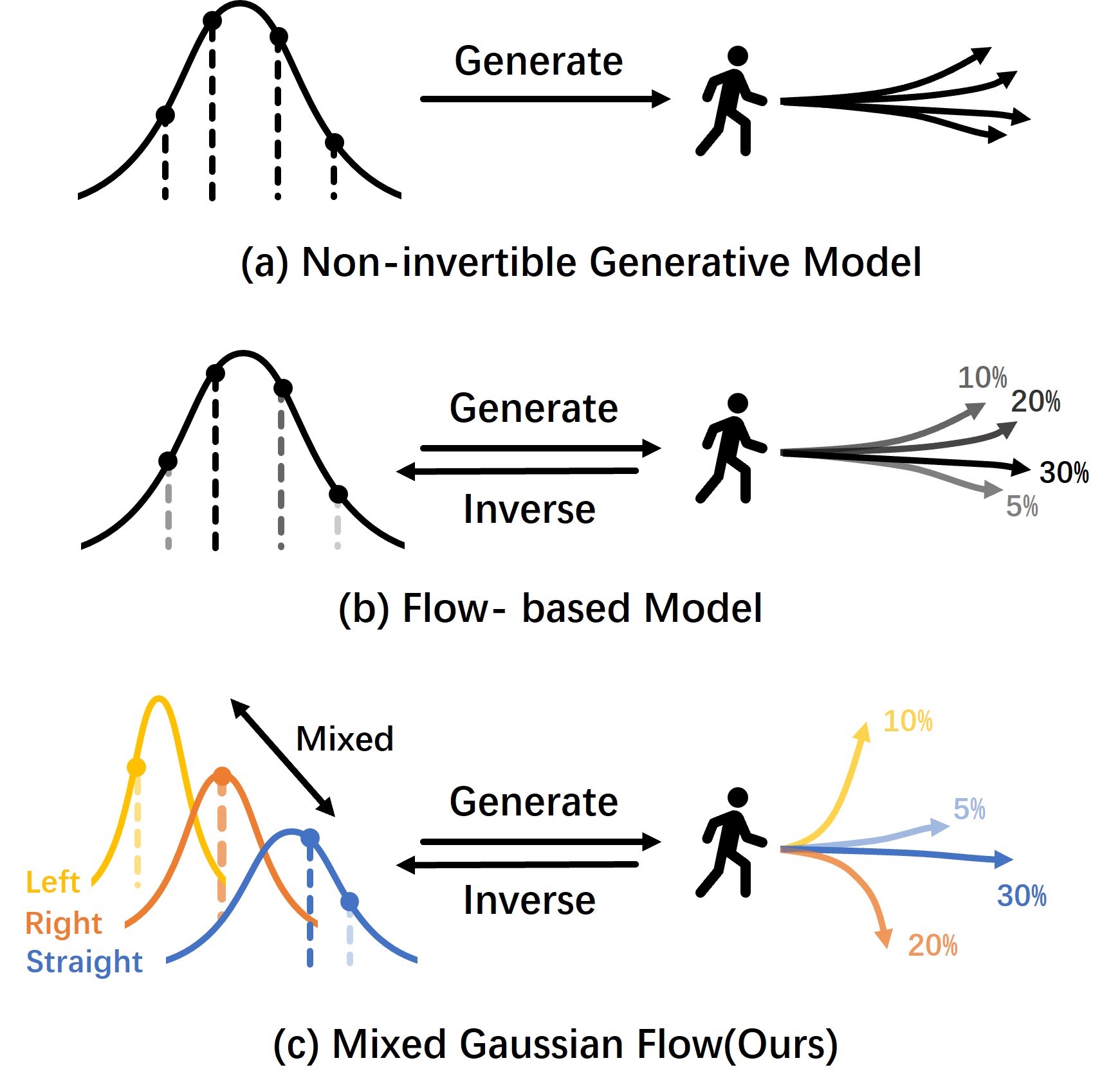
Figure 1: Non-invertible generative models (a), e.g., CVAE, GAN, and diffusions, lack the invertibility for probability density estimation. Flow-based methods (b) are invertible while, sampling from the symmetric standard Gaussian, undermines the diversity and controllability of generation. Our proposed Mixed Gaussian flow (c) maps from a mixed Gaussian prior instead. Summarizing distributions from data and controllable edits, it achieves better diversity and controllability for trajectory prediction.

From the perspective of learning from data, different motion patterns are usually imbalanced in a dataset. For example, agents are more likely to move straight than turn around in most cases. Many motion patterns are highly under-represented in the training data for trajectory prediction. This makes it challenging to learn a dense distribution of future trajectories with diverse motion patterns.

Moreover, many existing generative models solve the problem of trajectory prediction by transforming the target distribution from a simple and symmetric distribution, mostly standard Gaussian. This constrains the distribution of generated trajectories as some motion patterns are too sparse to be captured by the transformation.

Also, the popular evaluation metrics are calculated in a “best-of-$M$” fashion where only one candidate in a batch of M predictions is taken into the performance measurement. This protocol encourages the methods to generate outcomes similar to the mean (most likelihood) of the learned distribution to achieve a higher evaluation score.

Therefore, the combination of the bias from data, algorithm, and evaluation metrics significantly prevents the efforts to achieve good diversity in trajectory prediction. Our efforts in this work are motivated by this observation to achieve better diversity in probabilistic trajectory prediction. To allow more diverse trajectory prediction, we propose a Mixed Gaussian Flow (MGF) model under the theoretical framework of normalizing flow. Normalizing flow is a genre of generative models that maps from a single distribution to a complex one by a series of inevitable transformations. Compared to other non-inevitable generative models, normalizing flow allows the estimate of the marginal density of generation samples, which enhances the controllability and the explainability of the generation outcomes. Upon the standard normalizing flow, we propose to transform from a prior of mixed Gaussians instead of a single Gaussian. The mixed Gaussian prior is constructed by summarizing the motion patterns revealed in the training samples. Compared to the standard Gaussian, the mixture of Gaussians can better summarize the under-represented samples scattered far away in the representation space. This relieves the sparsity issue of rare cases when trying to learn diverse motion intentions. We demonstrate that the mixed Gaussian prior makes the normalizing flow-based methods easier to learn transformations to a broad space of the final distribution.

Given the constructed mixed Gaussian prior, MGF leverages a series of Continuously-indexed Flows (CIFs) to further enhance the flexibility of the generation process. The mixed Gaussian prior provides a more flexible resource for the initial noise sampling for normalizing flow. On the other hand, we adopt an history encoder in MGF to first transform the historical trajectories to a compact latent space for the later transformations by CIFs. We demonstrate empirically and qualitatively that the proposed architecture design improves the diversity of generated trajectories.

Besides diversity, our proposed method can also achieve better controllability of the generation results. This is because we construct the mixed Gaussian prior by first clustering trajectories into different sub-spaces, each of which reveals certain explainable motion intention. We could manipulate the sampling strategy or the mixed Gaussian prior to control the generation results. We could also insert or delete prior clusters to add or remove certain motion intention families. Because a compact set of parameters parametrizes the prior, we can do all these manipulations by editing the parametric distribution model instead of editing an intensive amount of data and no finetuning is needed.

Besides the efforts to enhance diversity by improving the data representation and algorithms, we also revise the evaluation metrics used in this community. To have an explicit measurement of generation outcome diversity, we propose a metric set of Average Pairwise Displacement (APD) and Final Pairwise Displacement (FPD). They measure the diversity of a batch of $M$ generated samples. This helps us to have a concrete study about generation diversity and avoid bias from the “best-of-$M$” evaluation protocol. We compare MGF with its closest baseline model FlowChain (Maeda & Ukita, 2023) to show that our method can improve the prediction diversity of models.

In this work, we focus on enhancing the diversity of the generated results for trajectory prediction. On the algorithm side, we propose Mixed Gaussian Flow (MGF) to achieve state-of-the-art alignment performance in both the “best-of-$M$” alignment metrics on multiple benchmarks and better diversity by applying the mixed Gaussian prior. On the evaluate metric side, we revise the bias of the popular “best-of-$M$” evaluation protocol and propose a new metric set to measure generation diversity explicitly. We have demonstrated that the proposed MGF model is capable of diverse and controllable trajectory predictions.

2 Related Works

Generative Models for Trajectory Prediction. Trajectory prediction, or trajectory forecasting, aims to predict the positions in a future horizon given historical position observations of multiple participants (agents). It has been studied widely in autonomous driving, robotics, intelligent city management, etc. Early studies solve the problem by deterministic trajectory prediction (Kitani et al., 2012). Social forces (Helbing & Molnar, 1995), RNNs (Alahi et al., 2016; Morton et al., 2016; Vemula et al., 2018), and the Gaussian Process (Wang et al., 2007) are proposed to model the agent motion intentions. On the other hand, recent works mostly seek multi-modal and probabilistic solutions for trajectory prediction. Though some of them leverage reinforcement learning (Li et al., 2021; Cao et al., 2021), the mainstream uses generative models to model the likely future trajectories. Auto-encoder (Kingma & Welling, 2013) and its variants, such as Conditional VAE (Lee et al., 2017; Yuan et al., 2021) are widely adopted. Also, Generative Adversarial Networks make another line of work (Gupta et al., 2018). Many of them use an encoder-decoder architecture for the generation (Li et al., 2022; Huang et al., 2019; Mohamed et al., 2020). And more recently, diffusion (Ho et al., 2020) model is also used in this area (Mao et al., 2023).

Normalizing Flow for Trajectory Prediction. In this work, we would like the predicted trajectories diverse and controllable. Therefore, we need the generation process can be invested and the marginal likelihood is tractable. We thus follow the line of work using generative normalizing flow (Kobyzev et al., 2020) for trajectory prediction. Normalizing flow (Papamakarios et al., 2021) is a method to construct complex distributions by transforming a probability density through invertible mappings. It transforms samples from one distribution, usually a simple one, such as Gaussian, to another, complex distribution. The transformation is performed by, implicitly or explicitly, computing the Jacobian mapping of the two distributions. When we use a deep network for the process, the calculation should be differentiable and the architecture is designed to be invertible. Normaling flow has been studied for trajectory prediction (Rhinehart et al., 2018, 2019; Guan et al., 2020). In the evaluation protocol of “best-of-$M$” trajectory candidates, normalizing flow-based methods are once considered not capable of achieving state-of-the-art performance. However, we will show in this paper that with proper design of architecture, normalizing flow can achieve on-par performance with state-of-the-art methods. And much more importantly, its invertibility allows more controllable and explainable trajectory prediction.

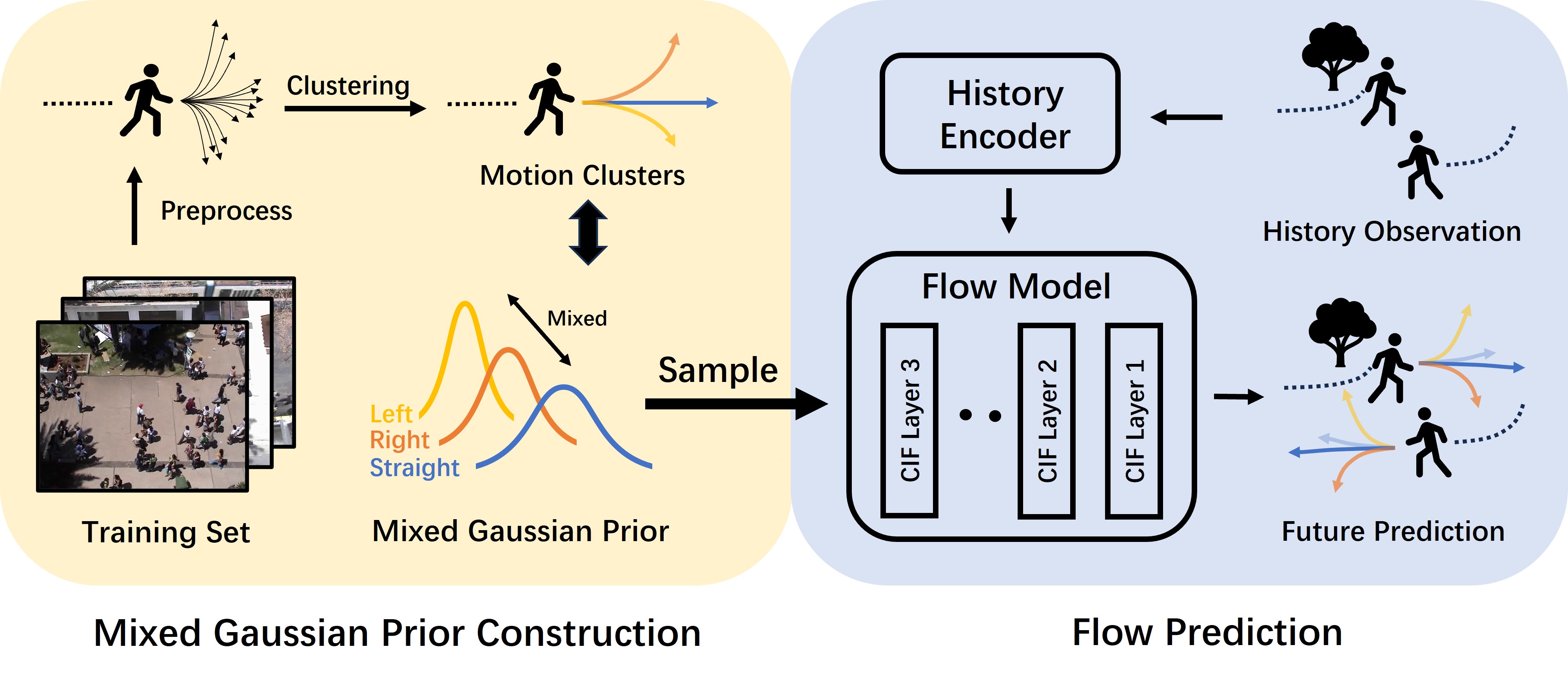
Figure 2: The illustration of our proposed Mixed Gaussian Flow (MGF) model. It has two stages. At the offline training stage, we will construct the mixed Gaussian prior by statistics from the training set. Then at the inference stage, the initial noise points from the flow model are sampled from the constructed mixed Gaussian prior instead of the naive Gaussian for a normal normalizing flow. Because the constructed mixed Gaussian prior is parameterized under a known parametric model thus its density is still tractable and MGF keeps the property of invertibility and marginal probability estimates.

3 Method

We first provide the formal problem formulation for trajectory prediction in Section 3.1 and introduce the preliminary about normalizing flow in Section 3.2. Then we explain the proposed Mixed Gaussian Flow (MGF) model in Section 3.3 and its training/inference implementations in Section 3.4. At last, we introduce the proposed metrics set to measure the diversity of generated trajectories in Section 3.5. The overall illustration of MGF is shown in Figure 2.

3.1 Problem Formulation

We follow the common practice of representing agent positions by 2D coordinates. We denote the 2D position of an agent $a$ at time $t$ as $\mathbf{x}_{t}^{a}$, the trajectory of $a$ from $t_{i}$ to $t_{j}$($t_{i}<t_{j}$) as $\mathbf{x}_{t_{i}:t_{j}}^{a}$. Given a fixed scene with map $\mathbf{M}$ and a period $\mathbf{T}$ from $t_{0}$ to $t_{2}$, there are $N$ agents that have appeared during the period $\mathbf{T}$, denoted as $A_{t_{0}:t_{2}}=\{a_{0},a_{1},...,a_{N-1}\}$. Without loss of generality, given a current timestep $t_{1}\in(t_{0},t_{2})$, the task of trajectory prediction aims to obtain a set of likely trajectories $\mathbf{x}_{t_{1}:t_{2}}^{a}$ with the past trajectories of all observed agents $\mathbf{x}_{t_{0}:t_{1}}^{A_{t_{0}:t_{1}}}=\{\mathbf{x}_{t_{0}:t_{1}}^{a},a\in A_{t_{0}:t_{1}}\}$ as input, where $a$ is an arbitrary agent that has shown up during $t:t_{0}\longrightarrow t_{1}$.

Therefore, the task of trajectory prediction seeks a solution for any observed agent $a\in A_{t_{0}:t_{1}}$ as

$$\mathbf{\hat{x}}_{t_{1}:t_{2}}^{a}=\Phi(\mathbf{x}_{t_{0}:t_{1}}^{A_{t_{0}:t_{1}}}),$$ (1)

at the same time, when there are other variables such as the observations of the maps are provided, we can use them as additional input information. By denoting the observations until $t$ as $\mathbf{O}_{t_{0}:t_{1}}$ we have

$$\mathbf{\hat{x}}_{t_{1}:t_{2}}^{a}=\Phi(\mathbf{x}_{t_{0}:t_{1}}^{A_{t_{0}:t_{1}}};\mathbf{O}_{t_{0}:t_{1}}).$$ (2)

If the generation process is probabilistic instead of deterministic, which we follow in this paper, the outcome of the solution is a set of trajectories instead of a single one. The formulation thus turns to

$$\{^{(i)}\mathbf{\hat{x}}_{t_{1}:t_{2}}^{a}\}=\Phi(\mathbf{x}_{t_{0}:t_{1}}^{A_{t_{0}:t_{1}}};\mathbf{O}_{t_{0}:t_{1}}),$$ (3)

where $i$ is the index of one candidate in the predicted batch.

For some generative models relying on transforming from a sample point in a known distribution $\mathcal{D}_{0}$ to the target distribution, for example, GANs and normalizing flows, the set is generated by mapping from different sample points, i.e., $p\in\mathcal{D}_{0}$. Therefore, the full formulation becomes

$$\{^{(i)}\mathbf{\hat{x}}_{t_{1}:t_{2}}^{a}\}=\Phi(\mathbf{x}_{t_{0}:t_{1}}^{A_{t_{0}:t_{1}}};\mathbf{O}_{t_{0}:t_{1}},\mathbf{P}),$$ (4)

where $\mathbf{P}=\{p_{0},...,p_{K}\}$ is a set of sampled points from $\mathcal{D}_{0}$. The formulation aligns with the practice of returning multiple candidates to prolong an existing trajectory by generative models from transforming from sampled noise.

3.2 Normaling Flow

Normalizing flow (Kobyzev et al., 2020) is a kind of generative model that constructs complex distributions by transforming a simple distribution through a series of invertible mappings. Let’s denote it as a bijective mapping $f$ which transforms a simple distribution $p(\mathbf{z})$ to a complex distribution $p(\mathbf{x})$. The transformation is often conditioned on context information $\mathbf{c}$. With the change-of-variables formula, we can derive as follows:

$$\mathbf{x} =f(\mathbf{z};\mathbf{c}),$$ (5)

$$p(\mathbf{x}) =p(\mathbf{z})\cdot|\det(\nabla_{\mathbf{x}}f^{-1}(\mathbf{x};\mathbf{c}))|,$$

$$-\log(p(\mathbf{x})) =-\log(p(\mathbf{z}))-\log(|\det(\nabla_{\mathbf{x}}f^{-1}(\mathbf{x};\mathbf{c}))|).$$

Given the formulations, with a known distribution $\mathbf{z}\sim\mathcal{D}_{0}$, we can calculate the density of $p(\mathbf{x})$ following the transformations and vice versa. However, the equations require the Jacobian determinant of the function $f$ to obtain the distribution density $p(\mathbf{x})$. The calculation of it in the high-dimensional space is not trivial. Recent works propose to use deep neural networks to approximate the Jacobians. To maintain the inevitability of the normalizing flows, some carefully designed layers are inserted into the deep models and the coupling layers (Dinh et al., 2016a) are one of the most widely adopted ones.

More recently, Flow-chain (Maeda & Ukita, 2023) is proposed to enhance the standard normalizing flow models by using a series of Conditional Continuously-indexed Flows (CIFs) (Cornish et al., 2020) to estimate future trajectory density. CIFs are obtained by replacing the single bijection $f$ in normalizing flows with an indexed family ${F(\cdot;u)}_{u\in U}$, where $U\subseteq R$ is the index set and each $F(\cdot;u):\mathbf{z}\longrightarrow\mathbf{x}$ is a bijection. Then, the transformation is changed to

$$\mathbf{z}\sim p(\mathbf{z}),\quad U\sim p_{U|\mathbf{z}}(\cdot|\mathbf{z}),\quad\mathbf{x}:=F(\mathbf{z};U).$$ (6)

Please refer to Cornish et al. (2020) for more details about CIFs and their connection with variational inference. In this work, we follow the idea of using a stack of CIFs from Maeda & Ukita (2023) to achieve fast inference and the updates of trajectory density estimates.

Normalizing flow based model samples from a standard Gaussian, $\mathbf{z}\sim\mathcal{N}(0,1)$, usually results in overfitting to the most-likelihood for trajectory prediction. The symmetry of the standard Gaussian forces the generative model to learn a constrained symmetric-like target distribution, which is usually disagreed by the data distribution. This typically results in degraded expressiveness of the model to fail to capture under-represented motion patterns from the data. Such a forced symmetric target distribution hurts the diversity of the generated trajectories.

3.3 Mixed Gaussian Flow (MGF)

We propose Mixed Gaussian Flow (MGF) to enhance the diversity and controllability in trajectory prediction. MGF consists of two stages as summarized in Figure 2. First, we construct the mixed Gaussian prior by fitting the parametric model of a combination of $K$ Gaussians, $\{\mathcal{N}(\mu_{k},\sigma_{k}^{2})\},(1\leq k\leq K)$, with the training set data samples. Then, during inference, we would sample points from the mixture of Gaussian and map them into a trajectory latent in the target distribution by a stack of CIF layers with the historical trajectories of all involved agents as the condition after being encoded by a history encoder. We will introduce the two stages in detail below.

MGF maps from a mixture of Gaussians instead of a single Gaussian to the target distribution, thus it can overcome the overfitting problem we mentioned in the normalizing flow section. However, to maintain the inevitability of the model, the mixed Gaussian prior can not be arbitrary. We obtain the parametric construction of the mixed Gaussian by fitting it with training data. In this fashion, we can derive multiple Gaussians to represent different motion patterns in the dataset, such as going straight or turning left and right. In a simplified perspective, we can regard the mixture as constructed from a combination of multiple clusters, each of which represents a certain sub-distribution. By sampling from the mixture of Gaussians instead of a standard Gaussian, our constructed model has more powerful expressiveness than the standard normalizing flow model. This results in more diverse trajectory predictions. Also, by manipulating the mixed Gaussian prior, we can achieve controllable trajectory prediction.

Mixed Gaussian Prior Construction. We first preprocess the trajectory annotations from the training datasets. Preprocessing transfers motion directions into relative directions with respect to a zero-degree direction. All position footage is represented in meters. Given the trajectory between $t_{0}\longrightarrow t_{1}$ to predict the trajectory between $t_{1}\longrightarrow t_{2}$, we would put the position pivot at $t_{1}$, i.e., $\mathbf{x}_{t_{1}}$, as the origin of the coordinate after preprocessing. Then, we would cluster the collection of future trajectory annotations into $K$ clusters, which is a hyper-parameter to decide here. We note the mean of the clusters as

$$\boldsymbol{\mu}=\{\mu_{i}\}_{i=1,...,K}.$$ (7)

These cluster centers reveal $K$ representative patterns of pedestrians’ motion, e.g. go straight, turn left. They will be the means of the Gaussians in the prior. And the variances of the Gaussian, i.e., $\sigma_{k}^{2}$, can be pre-determined or learned during the construction. The final mixture of Gaussians are denoted as

$$\mathcal{D}^{\Sigma}=\sum_{k=1}^{K}\beta_{k}\mathcal{N}(\mu_{k},\sigma_{k}^{2}),$$ (8)

where $\beta_{k}$ are the weighting factors to be decided from the training data. By default, we perform clustering by K-means with $K=8$.

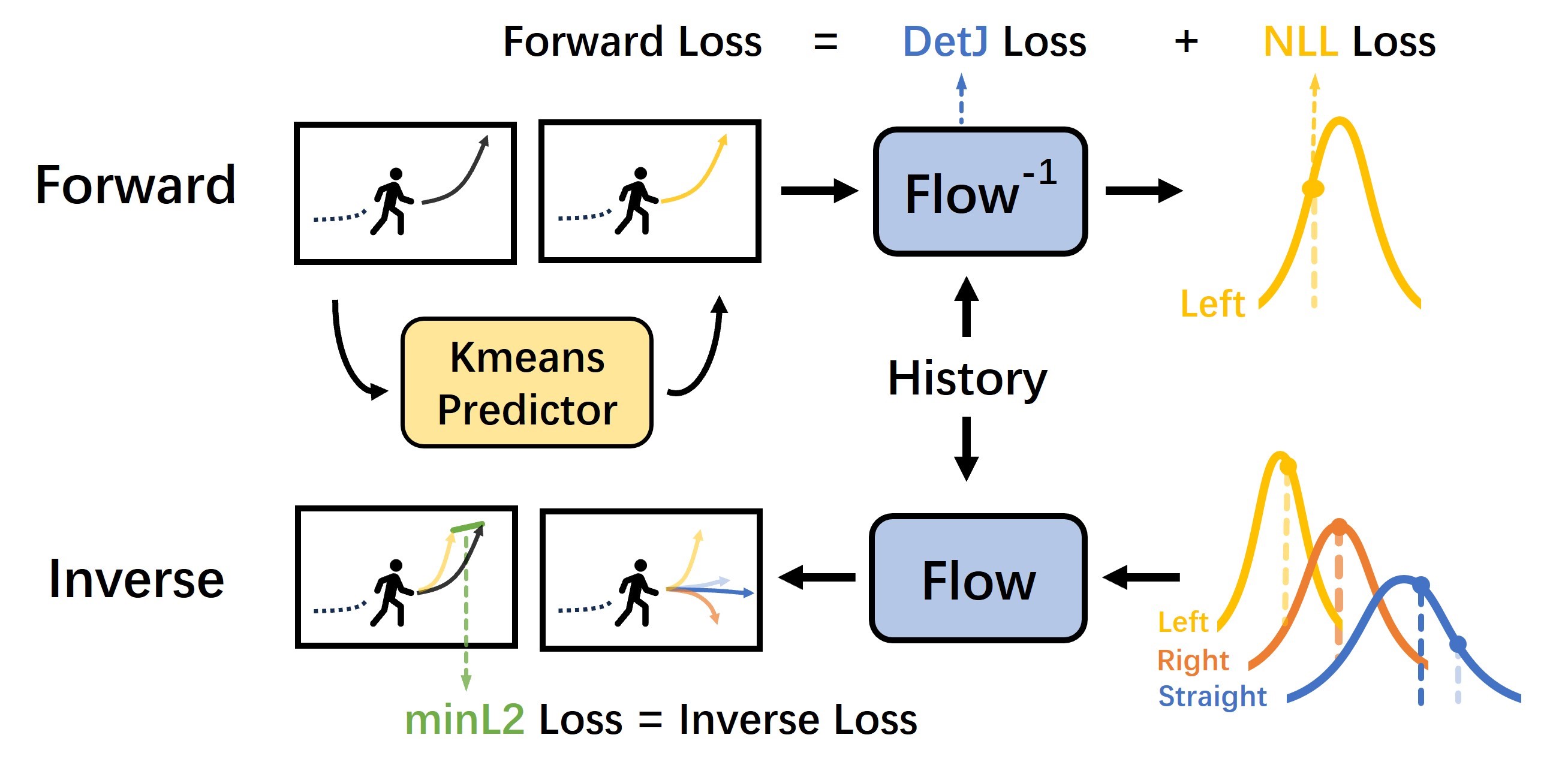
Figure 3: During training, the model is trained at both the forward process and the inverse process of the normalizing flow.

Flow Prediction. Once the mixed Gaussian prior is built, we can do trajectory prediction by mapping samples from the distribution to the target manifold for future trajectories. Here, we ignore the intermediate transformation by CIFs as Equation 6 shows while following the original formulations of normalizing flows as Equation 5 for simplicity. We distribute the samples from different Gaussians by their weights. Given the $i$-th sample from $\mathcal{N}(\mu_{k},\sigma_{k}^{2})$, we can transform it to the $i$-th predicted trajectories

$$\mathbf{z}_{i} \sim\mathcal{N}(\mu_{k},\sigma_{k}^{2}),$$ (9)

$${}^{(i)}\mathbf{\hat{x}}_{t_{1}:t_{2}}^{a} =\Phi(\mathbf{x}_{t_{0}:t_{1}}^{A_{t_{0}:t_{1}}};\mathbf{O}_{t_{0}:t_{1}},\mathbf{z}_{i}),$$

with the probability estimate

$$p(\mathbf{z}_{i})=\beta_{k}\frac{1}{\sigma_{k}\sqrt{2\pi}}e^{-\frac{(z_{i}-\mu_{k})^{2}}{2\sigma_{k}^{2}}},$$ (10)

it turns into

$$p(^{(i)}\mathbf{\hat{x}}_{t_{1}:t_{2}}^{a}) =\exp(-\frac{(z_{i}-\mu_{k})^{2}}{2\sigma_{k}^{2}}+\log\frac{\beta_{k}}{\sigma_{k}\sqrt{2\pi}})$$ (11)

$$\cdot|\det(\nabla_{f(\mathbf{z_{i}};\mathbf{O}_{t_{0}:t_{1}})}\mathbf{z_{i}})|,$$

which can be also invested back for the density estimate by the normalizing flow law

$$\hat{p}(\mathbf{z}_{i})=\beta_{k}\frac{1}{\sigma_{k}\sqrt{2\pi}}\exp({-\frac{[f^{-1}(^{(i)}{\hat{x}}_{t_{1}:t_{2}}^{a};{O}_{t_{0}:t_{1}})-\mu_{k}]^{2}}{2\sigma_{k}^{2}}}).$$ (12)

Table 1: Results on ETH/UCY dataset with Best-of-20 metrics. Scores are in meters, lower is better. bold and underlined scores denote the best and the second-best scores.

	ETH		HOTEL		UNIV		ZARA1		ZARA2		Mean
Method	ADE	FDE	ADE	FDE	ADE	FDE	ADE	FDE	ADE	FDE	ADE	FDE
Social-GAN (Gupta et al., 2018)	0.87	1.62	0.67	1.37	0.76	1.52	0.35	0.68	0.42	0.84	0.61	1.21
STGAT (Huang et al., 2019)	0.65	1.12	0.35	0.66	0.52	1.10	0.34	0.69	0.29	0.60	0.43	0.83
Social-STGCNN (Mohamed et al., 2020)	0.64	1.11	0.49	0.85	0.44	0.79	0.34	0.53	0.30	0.48	0.44	0.75
Trajectron++ (Salzmann et al., 2020)	0.61	1.03	0.20	0.28	0.30	0.55	0.24	0.41	0.18	0.32	0.31	0.52
MID (Gu et al., 2022)	0.55	0.88	0.20	0.35	0.30	0.55	0.29	0.51	0.20	0.38	0.31	0.53
PECNet (Mangalam et al., 2020)	0.54	0.87	0.18	0.24	0.35	0.60	0.22	0.39	0.17	0.30	0.29	0.48
GroupNet (Xu et al., 2022a)	0.46	0.73	0.15	0.25	0.26	0.49	0.21	0.39	0.17	0.33	0.25	0.44
AgentFormer (Yuan et al., 2021)	0.45	0.75	0.14	0.22	0.25	0.45	0.18	0.30	0.14	0.24	0.23	0.39
EqMotion (Xu et al., 2023)	0.40	0.61	0.12	0.18	0.23	0.43	0.18	0.32	0.13	0.23	0.21	0.35
FlowChain (Maeda & Ukita, 2023)	0.55	0.99	0.20	0.35	0.29	0.54	0.22	0.40	0.20	0.34	0.29	0.52
MGF(Ours)	0.40	0.59	0.15	0.25	0.23	0.41	0.17	0.29	0.14	0.24	0.22	0.35

Table 2: Results on SDD dataset with Best-of-20 metrics. Scores are in pixels.

Method	ADE	FDE
Social-GAN (Gupta et al., 2018)	27.25	41.44
STGAT (Huang et al., 2019)	14.85	28.17
Social-STGCNN (Mohamed et al., 2020)	20.76	33.18
Trajectron++ (Salzmann et al., 2020)	19.30	32.70
MID (Gu et al., 2022)	10.31	17.37
PECNet (Mangalam et al., 2020)	9.97	15.89
GroupNet (Xu et al., 2022a)	9.31	16.11
MemoNet (Xu et al., 2022b)	8.56	12.66
FlowChain (Maeda & Ukita, 2023)	9.93	17.17
MGF (Ours)	7.74	12.17

3.4 Training and Inference

Here, we introduce the training process of the proposed MGF model. The training loss comes from two directions: the forward process to get mixed flow loss and the inverse process to get minimum $\ell_{2}$ loss.

Forward process. Given a ground truth trajectory sample $\mathbf{x}_{t_{1}:t_{2}}^{a}$, we need to assign it to a cluster in the mixed Gaussian prior by measuring its distance to the centroids

$$\hat{k} =\mathop{\arg\min}_{i}(\mathbf{x}_{t_{1}:t_{2}}^{a}-\mu_{i})^{2},$$ (13)

$$p_{\hat{k}}(\cdot) =\beta_{\hat{k}}\mathcal{N}(\mu_{\hat{k}},\sigma_{\hat{k}^{2}}).$$

Through the inverse process $f^{-1}$ of flow model, we transform $\mathbf{x}_{t_{1}:t_{2}}^{a}$ into its corresponding latent representation, here denoted as

$$\mathbf{\hat{z}}=f^{-1}(\mathbf{x}_{t_{1}:t_{2}}^{a};\mathbf{O}_{t_{0}:t_{1}}).$$ (14)

Then we can compute the forward mixed flow loss:

$$L_{forward} =-\log(p(\mathbf{x}_{t_{1}:t_{2}}^{a}))$$ (15)

$$=-\log(p_{\hat{k}}(\mathbf{\hat{z}}))-\log(|\det(\nabla_{\mathbf{x}_{t_{1}:t_{2}}^{a}}\mathbf{\hat{z}})|).$$

Instead of computing negative-log-likelihood(NLL) loss of $\mathbf{\hat{z}}$ in the mixed distribution $\sum_{k=1}^{K}\beta_{k}\mathcal{N}(\mu_{k},\sigma_{k}^{2})$, we compute NLL loss in the sub-Gaussian with the nearest centroid $\beta_{\hat{k}}\mathcal{N}(\mu_{\hat{k}},\sigma_{\hat{k}^{2}})$ because each centroid is independent to others in the mixed distribution and we encourage the model to learn specified motion patterns to avoid overwhelming by the major data patterns. Calculating NLL loss over the mixed distribution may fuse other centroids and damage the diversity of model outputs. By our design, the mixed Gaussian prior can maintain more capacity of expressing complicated multi-modal distribution than the traditional single Gaussian prior, which typically constrains the target distribution to be single-modal and symmetric.

Inverse Process. This process repeats the flow prediction process to get generated trajectories. To predict $M$ candidates, we sample $\mathbf{z}_{i}\sim\sum_{k=1}^{K}\beta_{k}\mathcal{N}(\mu_{k},\sigma_{k}^{2}),i=1,2,...,M$ and transform them into $M$ trajectories

$$\{^{(i)}\mathbf{\hat{x}}_{t_{1}:t_{2}}^{a}\}=\{f(\mathbf{z}_{i};\mathbf{O}_{t_{0}:t_{1}})\},i=1,2,...,M.$$ (16)

We compute the minimum $\ell^{2}$ loss between $M$ predictions and ground truth trajectory as Gupta et al. (2018) does:

$$L_{inverse}=\min_{i=1}^{M}\frac{{(^{(i)}\mathbf{\hat{x}}_{t_{1}:t_{2}}^{a}-\mathbf{x}_{t_{1}:t_{2}}^{a}})^{2}}{t_{2}-t_{1}}.$$ (17)

We sample $\mathbf{z}_{i}$ from sub Gaussians by their weight. This is generally equal to sampling from the original mixed Gaussians but makes the reparameterization trick doable.

The forward and inverse losses encourage the model to predict a well-aligned sample in a sub-space from the prior without hurting the flexibility and expressiveness of other sub-spaces. Finally, we combine the forward and inverse losses to be a Symmetric Cross-Entropy loss (Rhinehart et al., 2018) by a ratio $\gamma$ for model training:

$$L=L_{forward}+\gamma\cdot L_{inverse}.$$ (18)

3.5 Diversity Metrics

The widely adopted ADE/FDE scores measure the agreement (alignment) between the ground truth future trajectory and one predicted trajectory. Under the common “best-of-$M$” evaluation protocol, ADE/FDE scores encourage generating a single “aligned” trajectory with the ground truth. Such an evaluation protocol overwhelmingly encourages the methods to fit the most likelihood from a certain distribution and all generated candidates race to be the most similar one as the distribution mean. However, this bias hurts one of the core objectives of probabilistic trajectory prediction methods, instead of deterministic ones, namely the diversity of predicted trajectory hypotheses.

To provide a tool for quantitative trajectory diversity evaluation, we add a set of metrics here. Following the idea of average displacement error (ADE) and final displacement error (FDE), we measure the diversity of trajectories by their pairwise displacement along the whole generated trajectories and the final step. We name that average pairwise displacement (APD) and final pairwise displacement (FPD). We note that the diversity metrics are measured in the complete set of generated trajectory candidates instead of between a single candidate and the ground truth. The formulation of APD and FPD are as below

$$\text{APD}=\frac{\sum_{i=1}^{M}\sum_{j=1}^{M}\sqrt{(^{(i)}\mathbf{\hat{x}}_{t_{1}:t_{2}}^{a}-^{(j)}\mathbf{\hat{x}}_{t_{1}:t_{2}}^{a})^{2}}}{M^{2}\cdot(t_{2}-t_{1})},$$ (19)

$$\text{FPD}=\frac{\sum_{i=1}^{M}\sum_{j=1}^{M}\sqrt{(^{(i)}\mathbf{\hat{x}}_{t_{2}}^{a}-^{(j)}\mathbf{\hat{x}}_{t_{2}}^{a})^{2}}}{M^{2}},$$ (20)

where APD measures the average displacement along the whole predicted trajectories and FPD measures the displacement of trajectory endpoints.

4 Experiments

We first introduce experiment setup to in Section 4.1 and benchmark with related works to evaluate the trajectory prediction alignment and diversity in Section 4.2. Then, we showcase the diversity and controllability of MGF in Section 4.3 and Section 4.4. Finally, we ablate key implementation components in Section 4.5.

4.1 Setup

Datasets. We evaluate on two major benchmarks: ETH/UCY (Lerner et al., 2007; Pellegrini et al., 2009) and SDD (Robicquet et al., 2016). ETH/UCY consists of five subsets: ETH, HOTEL, UNIV, ZARA1, and ZARA2. We follow the standard leave-one-out evaluation protocol and the widely-used train-validation-test split of Social-GAN (Gupta et al., 2018). SDD dataset consists of 20 scenes captured in bird’s eye view. We follow the preprocessed data and train-validation-test split of TrajNet (Sadeghian et al., 2018). Both datasets sample timesteps at 2.5Hz and take 8 timesteps (3.2s) past as observation to predict 12 timesteps (4.8s) into the future. We note that in the community of trajectory prediction, previous works have inconsistent evaluation protocol details and thus have made unfair comparisons. Please refer to Appendix A for details.

Table 3: Results on ETH/UCY dataset with diversity metrics. Scores are in meters, higher means more diverse prediction. bold and underlined scores denote the best and the second-best scores.

	ETH		HOTEL		UNIV		ZARA1		ZARA2		Mean
Method	APD	FPD	APD	FPD	APD	FPD	APD	FPD	APD	FPD	APD	FPD
Social-GAN (Gupta et al., 2018)	0.680	1.331	0.566	1.259	0.657	1.502	0.617	1.360	0.515	1.119	0.607	1.314
Social-STGCNN (Mohamed et al., 2020)	0.404	0.633	0.591	0.923	0.333	0.497	0.490	0.762	0.417	0.657	0.447	0.694
Trajectron++ (Salzmann et al., 2020)	0.704	1.532	0.568	1.240	0.648	1.404	0.697	1.528	0.532	1.161	0.630	1.373
AgentFormer (Yuan et al., 2021)	1.998	4.560	0.995	2.333	1.049	2.445	0.774	1.772	0.849	1.982	1.133	2.618
MemoNet (Xu et al., 2022b)	1.232	2.870	0.950	2.030	0.847	1.822	0.844	1.919	0.880	2.120	0.951	2.152
FlowChain (Maeda & Ukita, 2023)	0.814	1.481	0.484	0.833	0.636	1.094	0.505	0.890	0.492	0.859	0.586	1.031
MGF(Ours)	1.624	3.555	1.138	2.387	1.115	2.163	1.029	2.119	1.065	2.182	1.194	2.481

Table 4: minADE/minFDE of worst-$N$ predictions on UNIV dataset. By adding augmented data along with their corresponding cluster centers, our method significantly improves the performance on the corner cases.

	FlowChain		Augment-MGF
$N$	ADE	FDE	ADE	FDE
10	3.13	6.54	0.75	1.30
50	2.40	4.90	0.90	1.57
100	2.06	4.29	1.07	1.86

Metrics. We use widely used average displacement error (ADE) and final displacement error (FDE) to measure the alignment of the predicted trajectories and the ground truth. ADE is the average L2 distance between the ground truth and the predicted trajectory. FDE is the L2 distance between the ground truth endpoints and predictions. We follow the “Best-of-$M$” evaluation which computes the minimal ADE/FDE over $M$ predictions with $M=20$ as default. Besides the metrics for trajectory alignment, we also use the proposed diversity metrics set to measure the diversity of the predicted trajectory candidates.

Implementation Details. We enhance our model using a similar technique as “intension clustering" (Xu et al., 2022b) and we name it “prediction clustering". The key difference is that we directly cluster the entire trajectory instead of the endpoints. We utilized the data processing from FlowChain (Maeda & Ukita, 2023), which follows the data processing approach of Trajectron++ (Salzmann et al., 2020). To make a fair comparison, we follow the closet baseline (Maeda & Ukita, 2023) for the implementations of CIFs. Each CIF layer used three-layer RealNVP (Dinh et al., 2016b) with MLPs of 3 hidden layers and 128 hidden units. We use a Trajectron++ (Salzmann et al., 2020) encoder to encode historical trajectories.

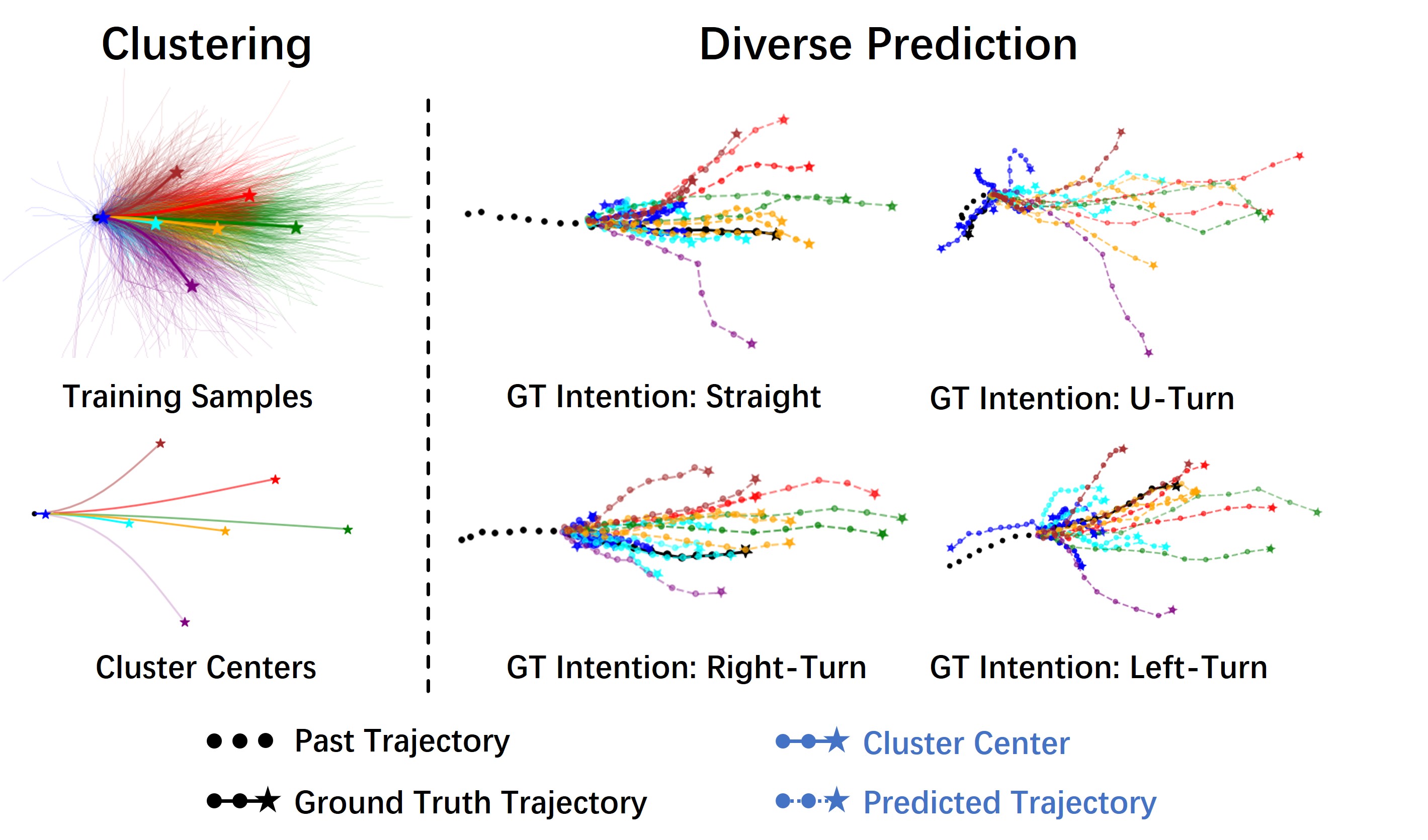
Figure 4: MGF predictions on ETH dataset. All colored trajectories are predicted by MGF. They correspond to the cluster centers from the mixed Gaussian prior to cover various motion patterns and also include candidates well aligned with the ground truth.

4.2 Benchmark Results

Table 5: Ablation study on the ETH/UCY and SDD dataset. All components are demonstrated beneficial to the prediction alignment.

				ETH/UCY		SDD
Inverse Loss	Mixed Gaussian	Learnable Variance	Prediction Clustering	ADE	FDE	ADE	FDE
				0.30	0.55	10.00	16.59
✓				0.29 ($\downarrow$0.01)	0.53 ($\downarrow$0.02)	9.65 ($\downarrow$0.35)	16.39 ($\downarrow$0.20)
✓	✓			0.28 ($\downarrow$0.01)	0.45 ($\downarrow$0.08)	9.26 ($\downarrow$0.39)	15.48 ($\downarrow$0.91)
✓	✓	✓		0.26 ($\downarrow$0.02)	0.42 ($\downarrow$0.03)	9.20 ($\downarrow$0.06)	14.78 ($\downarrow$0.70)
✓	✓	✓	✓	0.22 ($\downarrow$0.04)	0.36 ($\downarrow$0.06)	7.74 ($\downarrow$1.46)	12.17 ($\downarrow$2.61)

We benchmark MGF with a line of recent related works on ETH/UCY dataset in Table 1. The results of Trajectron++ and MID are updated according to a reported implementation issue . We can observe that MGF achieves on-par state-of-the-art performance. Specifically, Our method achieves the best ADE and FDE in 4 out of 5 splits and the best FDE score by averaging all splits. Our method significantly improves the performance compared to the closest baseline FlowChain, achieving 24.1% improvement by ADE and 32.7% improvement by FDE.

On the SDD dataset, we compare our method with existing methods as shown in Table 2. Our method outperforms all baselines measured by ADE/FDE for trajectory alignment. Specifically, Our method reduces ADE from 8.56 to 7.74 compared to the current state-of-the-art method, MemoNet, achieving 9.6% improvement. Our method also significantly improves the performance of FlowChain by 22.1% by ADE and 29.1% by FDE.

4.3 Diverse Generation

By leveraging the mixed Gaussian prior, our model can generate trajectories from the corresponding clusters, resulting in a more diverse set of trajectories.  Figure 4 shows that the generated trajectories of MGF cover various motion patterns. By sampling trajectories with the mixed Gaussian prior, we can also have a well-aligned candidate with the ground truth of different intentions. This figure explains why MGF can achieve good diversity (among all samples) and alignment (under the “best-of-$M$” protocol) at the same time.

We test the diversity metrics proposed in  Section 3.5 on ETH/UCY dataset, see  Table 3. We can observe that MGF achieves best or second-best APD and FPD score on all splits among sota methods. Besides, our method significantly improves the performance compared to FlowChain, achieving 103.7% improvement by APD and 140.6% improvement by FPD. Here the best APD/FPD checkpoints achieve slightly lower ADE/FDE score compared to the best ADE/FDE checkpoints.

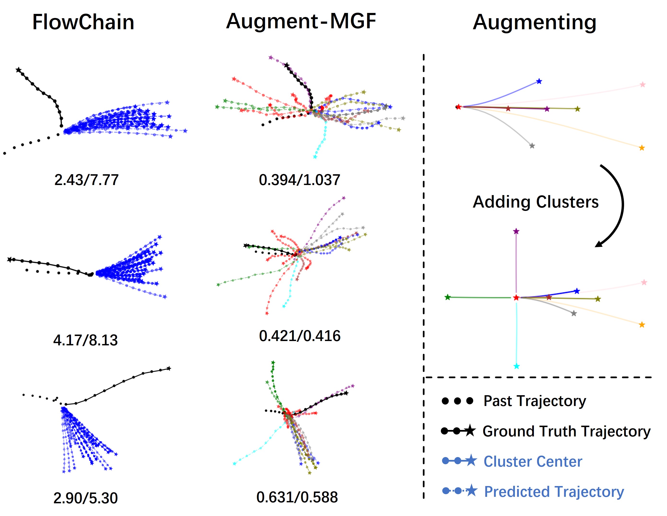
Figure 5: By adding augmented data along with their corresponding clusters, the model can generate corner cases that existing models fail to generate. We selected three examples from the UNIV dataset, namely left/right sharp turns and U-turns. The left column shows the predictions from FlowChain, while the middle column shows the predictions of MGF with augmented priors

4.4 Controllable Generation

By adjusting sub-Gaussians in the mixture prior, we can manipulate the generation process statistically. Figure 6 shows that by editing cluster compositions, we can control the predictions of MGF with good interpretability. Besides cluster centers, we can also edit the variance of Gaussian to control the density of generated trajectories or combine a set of operations to get expected predictions.

Further, we can use data augmentation to alter the data patterns in our training set, thereby obtaining different priors. This enables our model to fix corner cases that are difficult to handle with traditional flow-based models like FlowChain. On the other hand, we quantitatively evaluate the ability of generating under-represented trajectory patterns. Figure 5 shows the predictions of FlowChain and MGF on some typical corner cases. Table 4 compares the ADE/FDE scores of their worst-$N$ samples on the UNIV dataset. They demonstrate that, qualitatively and quantitatively, MGF can better generate the under-represented motion patterns.

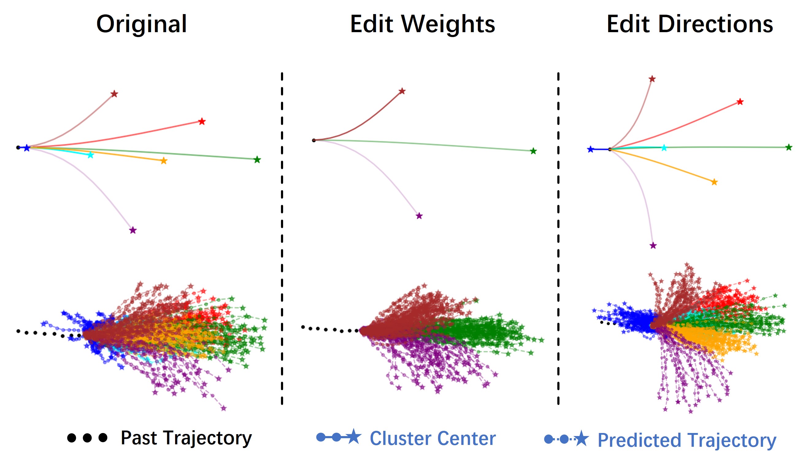
Figure 6: Controllable generation on ETH dataset. By editing the weights or intentions of cluster centers, we can flexibly control the predictions. We sample 500 trajectories for visualization.

4.5 Ablation Study

We ablate some key components of our implementation in Table 5. Flow-based models do not explicitly compute the loss in Euclidean space. We added an inverse loss to help improve ADE/FDE scores. Also, by replacing the prior distribution of the flow-based model from a standard Gaussian to our mixed Gaussian, we have demonstrated that the model generates more diverse outputs and achieves higher ADE/FDE scores. Also, by setting the variance of the mixed Gaussian prior as learnable, we find the ADE/FDE is also improved. Finally, prediction clustering as post-processing makes the “best-of-M” predictions from $L$ original predictions ($L>M$). The performance is also improved.

5 Conclusion

We improve the diversity of probabilistic trajectory prediction in this work. By revising the factors from data, algorithm, and metrics to discourage trajectory prediction diversity, we propose Mixed Gaussian Flow (MGF) model for the diverse and controllable trajectory generation. MGF reforms the normalizing flow model by using mixed Gaussian instead of a single Gaussian as the original distribution. We also propose a set of metrics to evaluate the diversity of generation candidates explicitly. Quantitative and qualitative experiments demonstrate the effectiveness of MGF.

Appendix A Inconsistent Practice of the Evaluation for Trajectory Prediction

Previous research has focused on multiple datasets for the quantitative evaluation of trajectory prediction methods. However, we notice that the evaluation settings of previous works are inconsistent thus making noisy and unfair comparisons in the benchmarks we usually refer to.

A.1 ETH/UCY benchmark

The ETH/UCY (Lerner et al., 2007; Pellegrini et al., 2009) datasets, comprising five subsets of data, serve as the primary benchmark for human trajectory prediction. However, the original dataset lacks benchmarks for data splitting and model evaluation metrics. Consequently, numerous prior studies employ different benchmarks, leading to unfair comparisons.

The benchmark widely adopted by the research community was initially proposed by Social-GAN (Gupta et al., 2018). It adheres to the following principles: 1. Utilizing data with a sampling rate of 10 in all subsets. 2. Employing a leave-one-out approach, where the model is trained on four sets and tested on the remaining set. 3. Further dividing the training data into train, eval and test sets. Subsequent works like Trajectron++ (Salzmann et al., 2020), AgentFormer (Yuan et al., 2021), and EqMotion (Xu et al., 2023) have widely embraced this benchmark and evaluation setting.

However, not all studies adhere to this benchmark. To identify examples, we conducted a review of recent open-access conference papers, which reveals the following divergence:

1. Sampling Rate on ETH dataset. There are two widely used sampling rates for the evaluation on the ETH dataset. While Social-GAN (Gupta et al., 2018) utilized the data with a sampling rate (SR) of 10FPS (SR=10), other works, such as SR-LSTM (Zhang et al., 2019), V2Net (Wong et al., 2023a), SocialCircle (Wong et al., 2023b), STAR (Yu et al., 2020), PCCSNet (Sun et al., 2021), Stimulus Verification (Sun et al., 2023), and MG-GAN (Dendorfer et al., 2021), used the version with a sampling rate of 6FPS (SR=6). The SR=6 version contains more data, with a total of 8,908 frames, whereas the SR=10 version consists of only 5,492 frames. Based on our experience, the same model tends to yield higher evaluation scores (ADE/FDE) on the SR=6 version compared to the SR=10 version.

2. Data Splitting. Social-GAN follows a specific scheme and ratio for splitting the data into train/val/test sets, while some works have adopted different conventions. For instance, Sophie (Sadeghian et al., 2019) selected fewer training scenes, MG-GAN (Dendorfer et al., 2021) used the complete training scene data for training while separating a portion of the test set for evaluation. Evidently, works utilizing the SR=6 and SR=10 versions of the ETH-eth dataset also diverge in their data splitting methods.

3. Inconsistent Processed Data. Some other studies, such as Y-Net (Mangalam et al., 2021), Introvert (Shafiee et al., 2021), and Next (Liang et al., 2019), provide processed data without the raw data and the processing scripts. The provided processed data for val/test sets does not align with the Social-GAN benchmark.

Therefore, there are multiple different evaluation protocol conventions on the ETH/UCY dataset. Because the data splitting for training/test and evaluation details are different, putting the evaluation numbers from them together provides misleading quantitative observations, which the community has been using for a while.

A.2 SDD benchmark

Compared to ETH/UCY, SDD (Robicquet et al., 2016) is a more recent dataset consisting of 20 scenes captured in bird’s eye view. SDD contains various moving agents such as pedestrians, bicycles, and cars.

Most works follow the setting of TrajNet (Sadeghian et al., 2018) which comes from a public challenge. However, some works adopt different evaluation way compared to TrajNet. SimAug (Liang et al., 2020) reprocesses the raw videos and gets a set of data files different from TrajNet. Besides, it used a different data splitting approach. Subsequent works such as V2Net (Wong et al., 2023a) and SocialCircle (Wong et al., 2023b) follow the same setting as SimAug. DAG-Net (Monti et al., 2021) shared the same data file with TrajNet, but used a different data splitting approach. Social-Implicit (Mohamed et al., 2022) followed its setting.

A.3 Summary

When comparing baseline results, many prior studies fail to meticulously verify whether they adhere to the same convention, thereby leading to unfair comparisons. To compare the performance of various models fairly, we recommend that the community adhere to the most widely used Social-GAN’s convention for ETH/UCY and TrajNet’s convention for SDD.

More specifically, for ETH/UCY dataset, we recommend to use the preprocessed data and dataloader from SocialGAN (Gupta et al., 2018)/Trajectron++ (Salzmann et al., 2020)/AgentFormer  (Yuan et al., 2021). For the SDD dataset, we recommend using the preprocessed data and dataloader from Y-Net (Mangalam et al., 2021). Although their data processing methods may differ, they share the same data source and data splitting approach, facilitating fair comparisons.

We also note that, in the early version of Trajectron++, a misuse of the np.gradient function during computation resulted in the model accessing future information. Rectifying this bug typically leads to a significant decrease in scores. Consequently, several Trajectron++-based studies have achieved improved scores.

References

- Alahi et al. (2016) Alahi, A., Goel, K., Ramanathan, V., Robicquet, A., Fei-Fei, L., and Savarese, S. Social lstm: Human trajectory prediction in crowded spaces. In Proceedings of the IEEE conference on computer vision and pattern recognition, pp. 961–971, 2016.
- Cao et al. (2021) Cao, J., Wang, X., Darrell, T., and Yu, F. Instance-aware predictive navigation in multi-agent environments. In 2021 IEEE International Conference on Robotics and Automation (ICRA), pp. 5096–5102. IEEE, 2021.
- Cornish et al. (2020) Cornish, R., Caterini, A., Deligiannidis, G., and Doucet, A. Relaxing bijectivity constraints with continuously indexed normalising flows. In International conference on machine learning, pp. 2133–2143. PMLR, 2020.
- Dendorfer et al. (2021) Dendorfer, P., Elflein, S., and Leal-Taixé, L. Mg-gan: A multi-generator model preventing out-of-distribution samples in pedestrian trajectory prediction. In Proceedings of the IEEE/CVF International Conference on Computer Vision, pp. 13158–13167, 2021.
- Dinh et al. (2016a) Dinh, L., Sohl-Dickstein, J., and Bengio, S. Density estimation using real nvp. arXiv preprint arXiv:1605.08803, 2016a.
- Dinh et al. (2016b) Dinh, L., Sohl-Dickstein, J., and Bengio, S. Density estimation using real nvp. arXiv preprint arXiv:1605.08803, 2016b.
- Gu et al. (2022) Gu, T., Chen, G., Li, J., Lin, C., Rao, Y., Zhou, J., and Lu, J. Stochastic trajectory prediction via motion indeterminacy diffusion. In Proceedings of the IEEE/CVF Conference on Computer Vision and Pattern Recognition, pp. 17113–17122, 2022.
- Guan et al. (2020) Guan, J., Yuan, Y., Kitani, K. M., and Rhinehart, N. Generative hybrid representations for activity forecasting with no-regret learning. In Proceedings of the IEEE/CVF Conference on Computer Vision and Pattern Recognition, pp. 173–182, 2020.
- Gupta et al. (2018) Gupta, A., Johnson, J., Fei-Fei, L., Savarese, S., and Alahi, A. Social gan: Socially acceptable trajectories with generative adversarial networks. In Proceedings of the IEEE conference on computer vision and pattern recognition, pp. 2255–2264, 2018.
- Helbing & Molnar (1995) Helbing, D. and Molnar, P. Social force model for pedestrian dynamics. Physical review E, 51(5):4282, 1995.
- Ho et al. (2020) Ho, J., Jain, A., and Abbeel, P. Denoising diffusion probabilistic models. Advances in neural information processing systems, 33:6840–6851, 2020.
- Huang et al. (2019) Huang, Y., Bi, H., Li, Z., Mao, T., and Wang, Z. Stgat: Modeling spatial-temporal interactions for human trajectory prediction. In Proceedings of the IEEE/CVF international conference on computer vision, pp. 6272–6281, 2019.
- Kingma & Welling (2013) Kingma, D. P. and Welling, M. Auto-encoding variational bayes. arXiv preprint arXiv:1312.6114, 2013.
- Kitani et al. (2012) Kitani, K. M., Ziebart, B. D., Bagnell, J. A., and Hebert, M. Activity forecasting. In Computer Vision–ECCV 2012: 12th European Conference on Computer Vision, Florence, Italy, October 7-13, 2012, Proceedings, Part IV 12, pp. 201–214. Springer, 2012.
- Kobyzev et al. (2020) Kobyzev, I., Prince, S. J., and Brubaker, M. A. Normalizing flows: An introduction and review of current methods. IEEE transactions on pattern analysis and machine intelligence, 43(11):3964–3979, 2020.
- Lee et al. (2017) Lee, N., Choi, W., Vernaza, P., Choy, C. B., Torr, P. H., and Chandraker, M. Desire: Distant future prediction in dynamic scenes with interacting agents. In Proceedings of the IEEE conference on computer vision and pattern recognition, pp. 336–345, 2017.
- Lerner et al. (2007) Lerner, A., Chrysanthou, Y., and Lischinski, D. Crowds by example. In Computer graphics forum, volume 26, pp. 655–664. Wiley Online Library, 2007.
- Li et al. (2021) Li, J., Yang, F., Ma, H., Malla, S., Tomizuka, M., and Choi, C. Rain: Reinforced hybrid attention inference network for motion forecasting. In Proceedings of the IEEE/CVF International Conference on Computer Vision, pp. 16096–16106, 2021.
- Li et al. (2022) Li, M., Chen, S., Shen, Y., Liu, G., Tsang, I. W., and Zhang, Y. Online multi-agent forecasting with interpretable collaborative graph neural networks. IEEE Transactions on Neural Networks and Learning Systems, 2022.
- Liang et al. (2019) Liang, J., Jiang, L., Niebles, J. C., Hauptmann, A. G., and Fei-Fei, L. Peeking into the future: Predicting future person activities and locations in videos. In Proceedings of the IEEE/CVF conference on computer vision and pattern recognition, pp. 5725–5734, 2019.
- Liang et al. (2020) Liang, J., Jiang, L., and Hauptmann, A. Simaug: Learning robust representations from simulation for trajectory prediction. In Computer Vision–ECCV 2020: 16th European Conference, Glasgow, UK, August 23–28, 2020, Proceedings, Part XIII 16, pp. 275–292. Springer, 2020.
- Maeda & Ukita (2023) Maeda, T. and Ukita, N. Fast inference and update of probabilistic density estimation on trajectory prediction. In Proceedings of the IEEE/CVF International Conference on Computer Vision, pp. 9795–9805, 2023.
- Mangalam et al. (2020) Mangalam, K., Girase, H., Agarwal, S., Lee, K.-H., Adeli, E., Malik, J., and Gaidon, A. It is not the journey but the destination: Endpoint conditioned trajectory prediction. In Computer Vision–ECCV 2020: 16th European Conference, Glasgow, UK, August 23–28, 2020, Proceedings, Part II 16, pp. 759–776. Springer, 2020.
- Mangalam et al. (2021) Mangalam, K., An, Y., Girase, H., and Malik, J. From goals, waypoints & paths to long term human trajectory forecasting. In Proceedings of the IEEE/CVF International Conference on Computer Vision, pp. 15233–15242, 2021.
- Mao et al. (2023) Mao, W., Xu, C., Zhu, Q., Chen, S., and Wang, Y. Leapfrog diffusion model for stochastic trajectory prediction. In Proceedings of the IEEE/CVF Conference on Computer Vision and Pattern Recognition, pp. 5517–5526, 2023.
- Mohamed et al. (2020) Mohamed, A., Qian, K., Elhoseiny, M., and Claudel, C. Social-stgcnn: A social spatio-temporal graph convolutional neural network for human trajectory prediction. In Proceedings of the IEEE/CVF conference on computer vision and pattern recognition, pp. 14424–14432, 2020.
- Mohamed et al. (2022) Mohamed, A., Zhu, D., Vu, W., Elhoseiny, M., and Claudel, C. Social-implicit: Rethinking trajectory prediction evaluation and the effectiveness of implicit maximum likelihood estimation. In European Conference on Computer Vision, pp. 463–479. Springer, 2022.
- Monti et al. (2021) Monti, A., Bertugli, A., Calderara, S., and Cucchiara, R. Dag-net: Double attentive graph neural network for trajectory forecasting. In 2020 25th International Conference on Pattern Recognition (ICPR), pp. 2551–2558. IEEE, 2021.
- Morton et al. (2016) Morton, J., Wheeler, T. A., and Kochenderfer, M. J. Analysis of recurrent neural networks for probabilistic modeling of driver behavior. IEEE Transactions on Intelligent Transportation Systems, 18(5):1289–1298, 2016.
- Papamakarios et al. (2021) Papamakarios, G., Nalisnick, E., Rezende, D. J., Mohamed, S., and Lakshminarayanan, B. Normalizing flows for probabilistic modeling and inference. The Journal of Machine Learning Research, 22(1):2617–2680, 2021.
- Pellegrini et al. (2009) Pellegrini, S., Ess, A., Schindler, K., and Van Gool, L. You’ll never walk alone: Modeling social behavior for multi-target tracking. In 2009 IEEE 12th international conference on computer vision, pp. 261–268. IEEE, 2009.
- Rhinehart et al. (2018) Rhinehart, N., Kitani, K. M., and Vernaza, P. R2p2: A reparameterized pushforward policy for diverse, precise generative path forecasting. In Proceedings of the European Conference on Computer Vision (ECCV), pp. 772–788, 2018.
- Rhinehart et al. (2019) Rhinehart, N., McAllister, R., Kitani, K., and Levine, S. Precog: Prediction conditioned on goals in visual multi-agent settings. In Proceedings of the IEEE/CVF International Conference on Computer Vision, pp. 2821–2830, 2019.
- Robicquet et al. (2016) Robicquet, A., Sadeghian, A., Alahi, A., and Savarese, S. Learning social etiquette: Human trajectory understanding in crowded scenes. In Computer Vision–ECCV 2016: 14th European Conference, Amsterdam, The Netherlands, October 11-14, 2016, Proceedings, Part VIII 14, pp. 549–565. Springer, 2016.
- Sadeghian et al. (2018) Sadeghian, A., Kosaraju, V., Gupta, A., Savarese, S., and Alahi, A. Trajnet: Towards a benchmark for human trajectory prediction. arXiv preprint, 2018.
- Sadeghian et al. (2019) Sadeghian, A., Kosaraju, V., Sadeghian, A., Hirose, N., Rezatofighi, H., and Savarese, S. Sophie: An attentive gan for predicting paths compliant to social and physical constraints. In Proceedings of the IEEE/CVF conference on computer vision and pattern recognition, pp. 1349–1358, 2019.
- Salzmann et al. (2020) Salzmann, T., Ivanovic, B., Chakravarty, P., and Pavone, M. Trajectron++: Dynamically-feasible trajectory forecasting with heterogeneous data. In Computer Vision–ECCV 2020: 16th European Conference, Glasgow, UK, August 23–28, 2020, Proceedings, Part XVIII 16, pp. 683–700. Springer, 2020.
- Shafiee et al. (2021) Shafiee, N., Padir, T., and Elhamifar, E. Introvert: Human trajectory prediction via conditional 3d attention. In Proceedings of the IEEE/cvf Conference on Computer Vision and Pattern recognition, pp. 16815–16825, 2021.
- Sun et al. (2021) Sun, J., Li, Y., Fang, H.-S., and Lu, C. Three steps to multimodal trajectory prediction: Modality clustering, classification and synthesis. In Proceedings of the IEEE/CVF International Conference on Computer Vision, pp. 13250–13259, 2021.
- Sun et al. (2023) Sun, J., Li, Y., Chai, L., and Lu, C. Stimulus verification is a universal and effective sampler in multi-modal human trajectory prediction. In Proceedings of the IEEE/CVF Conference on Computer Vision and Pattern Recognition, pp. 22014–22023, 2023.
- Vemula et al. (2018) Vemula, A., Muelling, K., and Oh, J. Social attention: Modeling attention in human crowds. In 2018 IEEE international Conference on Robotics and Automation (ICRA), pp. 4601–4607. IEEE, 2018.
- Wang et al. (2007) Wang, J. M., Fleet, D. J., and Hertzmann, A. Gaussian process dynamical models for human motion. IEEE transactions on pattern analysis and machine intelligence, 30(2):283–298, 2007.
- Wong et al. (2023a) Wong, C., Xia, B., Peng, Q., and You, X. Another vertical view: A hierarchical network for heterogeneous trajectory prediction via spectrums. arXiv preprint arXiv:2304.05106, 2023a.
- Wong et al. (2023b) Wong, C., Xia, B., and You, X. Socialcircle: Learning the angle-based social interaction representation for pedestrian trajectory prediction. arXiv preprint arXiv:2310.05370, 2023b.
- Xu et al. (2022a) Xu, C., Li, M., Ni, Z., Zhang, Y., and Chen, S. Groupnet: Multiscale hypergraph neural networks for trajectory prediction with relational reasoning. In Proceedings of the IEEE/CVF Conference on Computer Vision and Pattern Recognition, pp. 6498–6507, 2022a.
- Xu et al. (2022b) Xu, C., Mao, W., Zhang, W., and Chen, S. Remember intentions: Retrospective-memory-based trajectory prediction. In Proceedings of the IEEE/CVF Conference on Computer Vision and Pattern Recognition, pp. 6488–6497, 2022b.
- Xu et al. (2023) Xu, C., Tan, R. T., Tan, Y., Chen, S., Wang, Y. G., Wang, X., and Wang, Y. Eqmotion: Equivariant multi-agent motion prediction with invariant interaction reasoning. In Proceedings of the IEEE/CVF Conference on Computer Vision and Pattern Recognition, pp. 1410–1420, 2023.
- Yu et al. (2020) Yu, C., Ma, X., Ren, J., Zhao, H., and Yi, S. Spatio-temporal graph transformer networks for pedestrian trajectory prediction. In Computer Vision–ECCV 2020: 16th European Conference, Glasgow, UK, August 23–28, 2020, Proceedings, Part XII 16, pp. 507–523. Springer, 2020.
- Yuan et al. (2021) Yuan, Y., Weng, X., Ou, Y., and Kitani, K. M. Agentformer: Agent-aware transformers for socio-temporal multi-agent forecasting. In Proceedings of the IEEE/CVF International Conference on Computer Vision, pp. 9813–9823, 2021.
- Zhang et al. (2019) Zhang, P., Ouyang, W., Zhang, P., Xue, J., and Zheng, N. Sr-lstm: State refinement for lstm towards pedestrian trajectory prediction. In Proceedings of the IEEE/CVF Conference on Computer Vision and Pattern Recognition, pp. 12085–12094, 2019.