Rotation curves in protoplanetary disks with thermal stratification

Abstract

Context. In recent years the gas kinematics probed by molecular lines detected with ALMA has opened a new window to study protoplanetary disks. High spatial and spectral resolution observations have revealed the complexity of protoplanetary disk structure and correctly interpreting these data allow us to gain a better comprehension of the planet formation process.

Aims. We investigate the impact of thermal stratification on the azimuthal velocity of protoplanetary disks. High resolution gas observations are showing velocity differences between CO isotopologues, which cannot be adequately explained with vertically isothermal models. The aim of this work is to determine whether a stratified model can explain this discrepancy.

Methods. We analytically solve the hydrostatic equilibrium for a stratified disk and we derive the azimuthal velocity. We test the model with SPH numerical simulations and then we use it to fit for star mass, disk mass and scale radius of the sources in the MAPS sample. In particular, we use ¹²CO and ¹³CO datacubes.

Results. When thermal stratification is taken into account, it is possible to reconcile most of the inconsistencies between rotation curves of different isotopologues. A more accurate description of CO rotation curves provides a deeper comprehension of the disk structure. The best fit values of star mass, disk mass and scale radius becomes more realistic and in line with previous studies. In particular, the quality of the scale radius estimate significantly increases when adopting a stratified model. In light of our results, we compute the gas-to-dust ratio and the Toomre Q parameter. Within our hypothesis, for all the sources the gas-to-dust ratio appears higher but close to the standard value of 100, within a factor of 2. The Toomre Q parameter suggests that the disks are gravitationally stable $(Q>1)$, however the systems that show spirals presence are closer to the conditions of gravitational instability ($Q\sim 5$).

1 Introduction

Our understanding of the physical properties of protoplanetary disks has improved in recent years thanks to the Atacama Large Millimeter Array (ALMA) (ALMA Partnership et al. 2015). High spectral and spatial resolution gas observations enable us to probe density, temperature and velocity fields of protostellar disks, gaining unique information about their structure (Law et al. 2021; Calahan et al. 2021; Teague et al. 2022; Miotello et al. 2023; Pinte et al. 2023; Lodato et al. 2023). Recently, the large program Molecules with ALMA at Planet-forming Scales (MAPS) (Öberg et al. 2021) targeted five protoplanetary disks (MWC 480, IM Lup, GM Aur, HD 163296 and AS 209) in several molecular lines. For optically thick line emission, the gas temperature can be measured along the emission surface directly from the peak surface brightness of the channel maps (Law et al. 2021). Given the varying heights of these emitting layers surfaces, it is possible to infer the thermal structure in disks, proving the existence of a vertical thermal stratification in them (Dartois et al. 2003; Rosenfeld et al. 2013; Pinte et al. 2018), as expected from basic radiative transfer arguments (Chiang & Goldreich 1997; D’Alessio et al. 1998, 1999). Although disk models have usually been considered as vertically isothermal, the vertical gradient of temperature leads to considerable corrections in the calculation of density structure and azimuthal velocity, which results in several percent deviations from the Keplerian velocity (Rosenfeld et al. 2013). Accounting for such differences is important not only to infer stellar masses, but also to accurately constrain the disk pressure structure and disk mass. Such parameters are of high importance to interpret velocity deviations that may be the signposts of planets (Pinte et al. 2018; Rabago & Zhu 2021; Bollati et al. 2021; Izquierdo et al. 2021; Bae et al. 2021), dust trapping (Teague et al. 2018; Rosotti et al. 2020) or disk instabilities (Hall et al. 2020; Terry et al. 2022; Longarini et al. 2021; Barraza-Alfaro et al. 2021).

In this paper, we analytically derive the density and velocity field of protostellar disks with thermal stratification, generalizing the work of Takeuchi & Lin (2002). A similar analysis of MAPS data with vertically isothermal disks have been performed by Lodato et al. (2023). We test the model against hydrodynamical simulations and we apply it to the whole MAPS sample for ¹²CO and ¹³CO data. In Sect. 2 we present the model, solving the vertical hydrostatic equilibrium and obtaining an expression for the azimuthal velocity. In Sect. 3 we present the numerical setup and the comparison between model and simulations. In Sect. 4 we apply the model and we discuss our findings. Finally, in Sect. 5 we compute the gas-to-dust ratio and the Toomre Q parameter and we draw our conclusions.

2 Model

2.1 Assumptions

In our analytical calculations, we do not make any assumption on the surface density $\Sigma$, considering it as arbitrary. However, in order to apply the model to observations, we are forced to choose a parameterization for the surface density and we assume that it is described by the self-similar solution of Lynden-Bell & Pringle (1974)

$$\Sigma=\frac{(2-\gamma)M_{\text{d}}}{2\pi R_{\text{c}}^{2}}\Bigg{(}\frac{R}{R_{\text{c}}}\Bigg{)}^{-\gamma}\exp\Bigg{[}-\Bigg{(}\frac{R}{R_{\text{c}}}\Bigg{)}^{2-\gamma}\Bigg{]},$$ (1)

where $M_{\text{d}}$ and $R_{\text{c}}$ are the disk mass and the scale radius respectively, $R$ is the cylindrical radius and $\gamma$ is a free parameter describing the steepness of the surface density. The disk density at the midplane $\rho_{\text{mid}}$ is

$$\rho_{\text{mid}}=\frac{\Sigma}{\sqrt{2\pi}H_{\text{mid}}}\propto R^{-(\gamma+(3-q)/2)}\exp\Bigg{[}-\Bigg{(}\frac{R}{R_{\text{c}}}\Bigg{)}^{2-\gamma}\Bigg{]},$$ (2)

where $H_{\text{mid}}=c_{\text{s},\text{mid}}/\Omega_{\text{k}}$ is the typical scale height of the disk at the midplane, $c_{\text{s},_{\text{mid}}}=\sqrt{k_{\text{b}}T_{\text{mid}}/(\mu m_{\text{p}})}\propto R^{-q/2}$ is the sound speed at the disk midplane, $k_{\text{b}}$ is the Boltzmann constant, $T_{\text{mid}}=T_{\text{mid},100}({R}/{100\text{au}})^{-q}$ is the temperature at midplane, $\mu$ is the mean molecular weight (usually assumed to be 2.1), $m_{\text{p}}$ is the proton mass and $\Omega_{\text{k}}=\sqrt{GM_{\star}/R^{3}}$ is the Keplerian angular velocity ($G$ is the gravitational constant and $M_{\star}$ is the stellar mass).

From literature (Chiang & Goldreich 1997; Dullemond et al. 2020) and observational data (Rosenfeld et al. 2013; Pinte et al. 2018; Law et al. 2021), we know that protoplanetary disks are thermally stratified. We take this into account by defining a function $f$ that describes the dependency of the temperature $T$ on height such that

$$T(R,z)=T_{\text{mid}}(R)f(R,z),$$ (3)

$$c_{\text{s}}^{2}(R,z)=c_{\text{s},\text{mid}}^{2}(R)f(R,z).$$ (4)

We underline that the isothermal case can be obtained considering $f\equiv 1$, thus $T=T_{\text{mid}}(R)$. As for the density, we assume that

$$\rho=\rho(R,z)=\rho_{\text{mid}}(R)g(R,z),$$ (5)

where $g$ describes how the density changes vertically. Note that in order to smoothly connect the functions above to their value at midplane it is necessary that $f(z=0)=1=g(z=0)$. Assuming a barotropic fluid, the pressure $P$ is given by

$$P(R,z)=P_{\text{mid}}(R)fg(R,z)=c_{\text{s},\text{mid}}^{2}(R)\rho_{\text{mid}}(R)fg(R,z).$$ (6)

While the profile of $f$ is arbitrary, this does not hold for $g$, whose value is set by solving the vertical hydrostatic equilibrium.

2.2 Hydrostatic equilibrium and rotation curve

To compute the vertical density profile we assume a non-self-gravitating disk under the condition of hydrostatic equilibrium in the vertical direction:

$$\frac{1}{\rho}\frac{dP}{dz}=-\frac{d\Phi_{\star}}{dz},$$ (7)

where $\Phi_{\star}=-GM_{\star}/r$ is the stellar potential ($r=\sqrt{R^{2}+z^{2}}$ is the spherical radius). Equation (7) can be written as (for further details see Appendix A):

$$c_{\text{s},_{\text{mid}}}^{2}f\frac{d\log(fg)}{dz}=-\Omega_{\text{k}}^{2}z\Bigg{[}1+\Bigg{(}\frac{z}{R}\Bigg{)}^{2}\Bigg{]}^{-3/2}.$$ (8)

Solving for $\log(fg)$, we find

$$\log(fg)=-\frac{1}{H_{\text{mid}}^{2}}\int_{0}^{z}\frac{z^{\prime}}{f}\left[1+\left(\frac{z^{\prime}}{R}\right)^{2}\right]^{-3/2}dz^{\prime}$$ (9)

and hence the density is given by

$$\rho(R,z)=\frac{\rho_{\text{mid}}(R)}{f(R,z)}\exp\left\{-\frac{1}{H_{\text{mid}}^{2}}\int_{0}^{z}\frac{z^{\prime}}{f(R,z^{\prime})}\left[1+\left(\frac{z^{\prime}}{R}\right)^{2}\right]^{-3/2}dz^{\prime}\right\}.$$ (10)

Assuming the condition of centrifugal balance, the rotation curve is given by the radial component of Navier-Stokes equation

$$v_{\phi}^{2}(R,z)=\frac{R}{\rho}\frac{dP}{dR}(R,z)+R\frac{d\Phi_{\star}}{dR}(R,z).$$ (11)

The first term in Eq.(11) can be written as (for further details see Appendix A)

$$\frac{R}{\rho}\frac{dP}{dR}=c_{\text{s},_{\text{mid}}}^{2}f\Bigg{[}\frac{d\log P_{\text{mid}}}{d\log R}+\frac{d\log(fg)}{d\log R}\Bigg{]},$$ (12)

and the second one as

$$R\frac{d\Phi_{\star}}{dR}(R,z)=v_{\text{k}}^{2}\left[1+\left(\frac{z}{R}\right)^{2}\right]^{-3/2},$$ (13)

where $v_{\text{k}}=\sqrt{GM_{\star}/R}$ is the Keplerian velocity. Therefore, the rotation curve is

$$\begin{split}v_{\phi}^{2}(R,z)=v_{\text{k}}^{2}\left\{\left[1+\left(\frac{z}{R}\right)^{2}\right]^{-3/2}+\left[\frac{d\log P_{\text{mid}}}{d\log R}+\right.\right.\\ \left.\left.+\frac{\text{d}\log(fg)}{\text{d}\log R}\right]\left(\frac{H}{R}\right)_{\text{mid}}^{2}f(R,z)\right\},\end{split}$$ (14)

which in the self-similar case becomes

$$\begin{split}v_{\phi}^{2}(R,z)=v_{\text{k}}^{2}\left\{\left[1+\left(\frac{z}{R}\right)^{2}\right]^{-3/2}-\left[\gamma^{\prime}+(2-\gamma)\left(\frac{R}{R_{c}}\right)^{2-\gamma}-\right.\right.\\ \left.\left.-\frac{\text{d}\log(fg)}{\text{d}\log R}\right]\left(\frac{H}{R}\right)_{\text{mid}}^{2}f(R,z)\right\},\end{split}$$ (15)

where $\gamma^{\prime}=\gamma+(3+q)/2$. Each term of Eq. (15) can be easily interpreted: $[1+(z/R)^{2}]^{-3/2}$ is the star contribution at the height $z$, $\gamma^{\prime}$ is the effect of the power law scaling of the pressure, $(2-\gamma)(R/R_{c})^{2-\gamma}$ is the effect of the exponential truncation and the logarithmic term is the effect of the vertical stratification. Since the latter is the derivative of a product, we do not know a priori its sign and thus if the rotation is accelerated or slowed down by thermal stratification (see Appendix A). In any case, in all our attempts this term never dominates over the variation of gravity with $z$. Thus, we found rotation to slow down with z and this effect is more pronounced as compared to the isothermal case when considering the parameters of the MAPS sample.

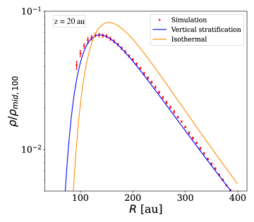
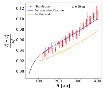
Figure 1: Comparison between the analytical models and the simulation after 8 outer orbits and at $z=20$au. Left panel: density field. Right panel: pressure gradient term of the rotation curve. The red dots represent the simulation data, while the blue and orange line show the thermally stratified model and the isothermal one respectively. The model with thermal stratification matches very well the simulation.

We underline that for the isothermal case ($f\equiv 1$), this expression reduces to the one derived and analyzed by Lodato et al. (2023), while Eq. (9) simplifies as:

$$\log g=-\frac{1}{H_{\text{mid}}^{2}}\int_{0}^{z}\frac{z^{\prime}dz^{\prime}}{[1+(z^{\prime}/R)^{2}]^{3/2}}=-\frac{R^{2}}{H_{\text{mid}}^{2}}\left(1-\frac{1}{\sqrt{1+z^{2}/R^{2}}}\right).$$ (16)

Therefore, the density in the isothermal case is given by:

$$\rho(R,z)=\rho_{\text{mid}}(R)\exp\left[\frac{R^{2}}{H_{\text{mid}}^{2}}\left(\frac{1}{\sqrt{1+z^{2}/R^{2}}}-1\right)\right].$$ (17)

If the disk is self-gravitating, we should add to the right-hand side of Eq.(11) the self-gravitating term (Bertin & Lodato 1999):

$$\begin{gathered}\frac{R}{\rho}\frac{d\Phi_{\text{d}}}{dR}(R,z)=G\int^{\infty}_{0}\Bigg{[}K(k)-\frac{1}{4}\Bigg{(}\frac{k^{2}}{1-k^{2}}\Bigg{)}\times\\ \Bigg{(}\frac{r}{R}-\frac{R}{r}+\frac{z^{2}}{Rr}\Bigg{)}E(k)\Bigg{]}\sqrt{\frac{r}{R}}k\Sigma(r)dr,\end{gathered}$$ (18)

where $K(k)$ and $E(k)$ are complete elliptic integrals (Abramowitz & Stegun 1970) and $k^{2}=4Rr/[(R+r)^{2}+z^{2}]$.

2.3 Temperature prescriptions

The two parameterizations of the vertical temperature more often used are given by Dartois et al. (2003) and Dullemond et al. (2020). In this work we will use the one by Dullemond et al. (2020), which is given by:

$$T(R,z)^{4}=T_{\epsilon}^{4}(R)+\frac{1}{2}T_{\text{atm}}^{4}(R)\Bigg{[}1+\tanh\Big{(}\frac{z}{Z_{q}(R)}-\alpha\Big{)}\Bigg{]}$$ (19)

and thus

$$f(R,z)=\Bigg{\{}\left(\frac{T_{\epsilon}}{T_{\text{mid}}}\right)^{4}+\frac{1}{2}\left(\frac{T_{\text{atm}}}{T_{\text{mid}}}\right)^{4}(R)\Bigg{[}1+\tanh\Big{(}\frac{z}{Z_{q}(R)}-\alpha\Big{)}\Bigg{]}\Bigg{\}}^{1/4},$$ (20)

where the atmospheric temperature is parameterized as $T_{\text{atm}}(R)=T_{\text{atm},100}({R}/{100\text{au}})^{-q_{\text{atm}}}$, $T_{\epsilon}$ is considered as an approximation of the temperature at midplane $T_{\epsilon}\simeq T_{\text{mid}}$, $Z_{q}(R)$ is defined as $Z_{q}(R)=\zeta_{100}(R/100\text{au})^{\beta}$ and $\alpha$ is a parameter that describes where the transition from midplane to atmospheric temperature occurs in the vertical direction. We note that in this case $f(R,z=0)\neq 1$ and thus the temperature does not smoothly connect to its value at midplane. We discuss this in Appendix B, but we underline that Eq. (19) is a good approximation for the five disks within the MAPS large program in most of the radial extent of the disk.

Once the function $f$ is defined, Eqs. (10) and (14) can be solved semi-analytically and completely specify the rotation curve. We have implemented this calculation in DYSC.

3 Comparison with numerical simulations

In this work, we performed numerical Smoothed Particle Hydrodynamics (SPH) simulations of protostellar disks using the code phantom (Price et al. 2018). This code is widely used in the astrophysical community to study gas and dust dynamics in accretion disks (Dipierro et al. 2015; Ragusa et al. 2017; Curone et al. 2022) and recently it has also been employed for kinematical studies (Pinte et al. 2018; Hall et al. 2020; Terry et al. 2022; Verrios et al. 2022). The aim of this simulation is to test the model before applying it to actual data.

To test the analytical model, we simulated a thermally stratified disk using the parameters of MWC 480 presented in Law et al. (2021). The simulation has been performed with $N=10^{6}$ gas particles, initially distributed as a tapered power law density profile, smoothed at inner radius, with $\gamma=1$ and $R_{c}=150$au, between $R_{\text{in}}=10$au and $R_{\text{out}}=400$au. The mass of the star is $2.1\text{M}_{\odot}$. For the temperature structure we used the Dullemond prescription given by Eq. (19), with $\zeta_{0}=7\text{au},\alpha=2.78,\beta=-0.05,T_{\text{mid},100}=27$K, $q=0.23$, $T_{\text{atm,100}}=69$K, $q_{\text{atm}}=0.7$. The $\alpha_{\text{SS}}$ Shakura & Sunyaev (Shakura & Sunyaev 1973) viscosity coefficient has been set to 0.005. No self gravity or dust have been included in the simulation.

We let the system evolve and reach hydrostatic equilibrium. We observed that after a couple of orbits the system reaches a relaxed state. We decided to analyze the output of the simulation after 8 outer orbits $(\sim 45\text{kyr})$. In Fig. 1 we show a comparison between the density and the velocity of the simulations (red dots) at $z=20$ au and both the isothermal and stratified model predictions. The red dots represent the azimuthal average of the respective quantity computed by averaging over all SPH particles within each of the 50 radial bins and the error bar is the corresponding standard deviation. Since we are plotting quantities at z = 20 au, we have excluded the inner points because at those radii (R ¡ 100 au) the disk has a smaller hydrostatic height H, causing numerical issues in the resolution of our simulation. The stratified model perfectly describes the density and the velocity field of the simulation and is a significant improvement over the isothermal one. In particular, in the right panel of Fig. 1 we see that the difference between the azimuthal velocity and the Keplerian velocity $(v_{\text{k}}^{2}-v_{\phi}^{2})/v_{\text{k}}^{2}$ reaches the $10-12\%$ and only the stratified model is able to reproduce it.

4 Applying the model

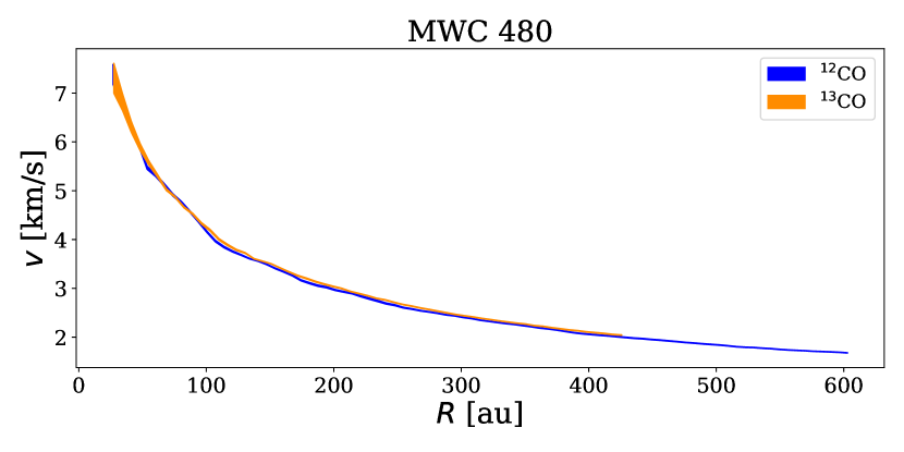
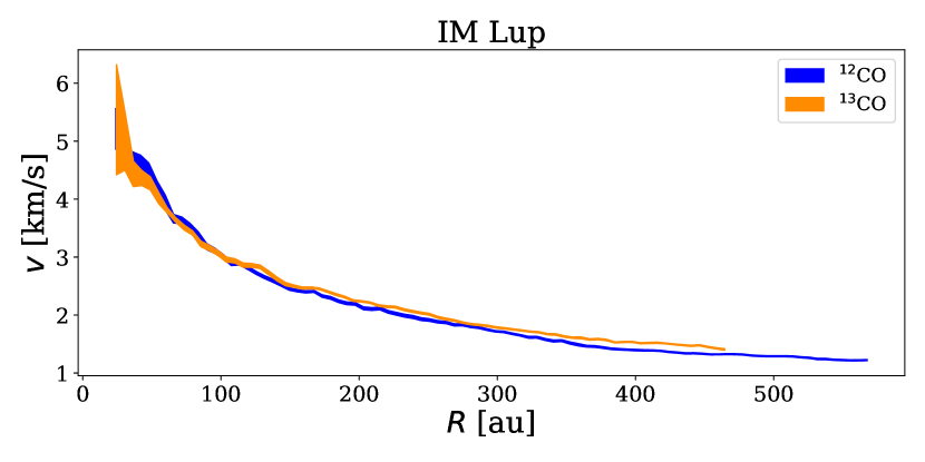
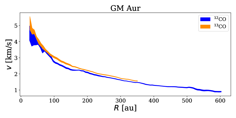
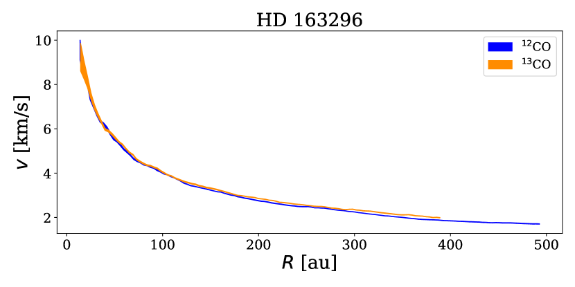
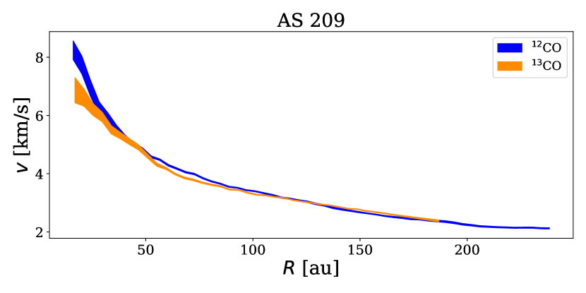
Figure 2: ¹²CO and ¹³CO rotation curves of the MAPS disks extracted with discminer.

4.1 The curves

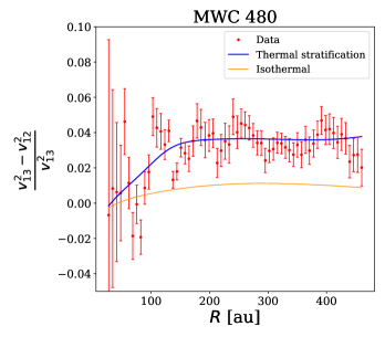
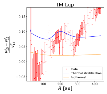
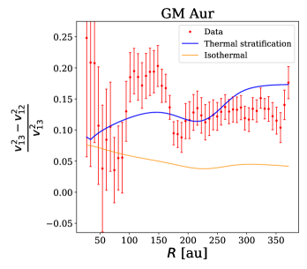
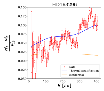
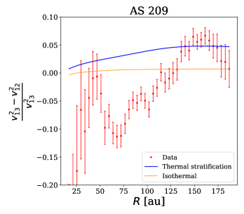
Figure 3: Relative difference between the squares of observed ¹²CO and ¹³CO rotation curves predicted by the thermally stratified model (blue line), the isothermal model (orange line) and the data (red dots). Except for AS 209, where this quantity is negative in the inner part, it is clearly visible that data are well reproduced by the stratified model. Indeed, the difference of speed between the two curves cannot be explained just in terms of different height.

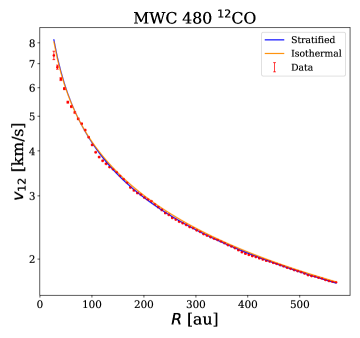
Figure 4: Left panel: rotation curve of MWC 480 obtained from ¹²CO data (red points), along with our best fitting curve for the stratified model (blue line) and the isothermal one (orange line). Right panel: same for the ¹³CO data.

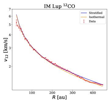
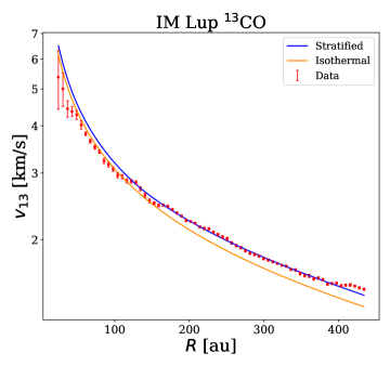
Figure 5: Same as figure 4 but for IM Lup.

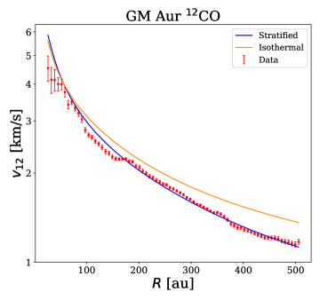
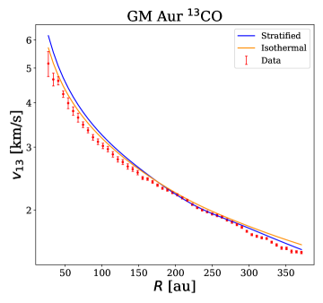
Figure 6: Same as figure 4 but for GM Aur.

In this section, we applied the model to the entire sample of disks from the MAPS ALMA Large Program (Öberg et al. 2021). We performed our fits under the assumption of vertically isothermal or stratified disk in order to compare the results. For the vertically isothermal model, the thermal structure is defined by the hydrostatic height of the disk at $R=100$au and the power law coefficient of the temperature profile $q$. These parameters are taken by Zhang et al. (2021). As for the stratified model, Law et al. (2021) obtained the two-dimensional temperature structure of the MAPS disks, using the Dullemond et al. (2020) prescription given by Eq. (19). Note that the rotation curve traced by a specific molecule is defined by

$$v_{\text{rot}}^{2}(R)=v_{\phi}^{2}(R,z(R)),$$ (21)

where $z(R)$ is the height of the emitting layer of the considered molecule. For the emitting layer, we use

$$z(R)=z_{0}\left(\frac{R}{100\text{au}}\right)^{\psi}\exp\left[-\left(\frac{R}{R_{t}}\right)^{q_{t}}\right],$$ (22)

where the best fit parameters have been obtained by Izquierdo et al. (2023). All the parameters used are summarized in Table 1.

Table 1: Velocity extraction method, orientation parameters, thermal parameters and emitting surfaces for ¹²CO and ¹³CO data of the MAPS disks. The orientation parameters and the emitting surfaces are taken from Izquierdo et al. (2023), the thermal parameters for the isothermal model are taken from Zhang et al. (2021), for the stratified model from Law et al. (2021).

	MWC 480	IM Lup	GM Aur	HD 163296	AS 209
Extraction
12CO	Gauss	Dbell	Dbell	Dbell	Gauss
13CO	Gauss	Dbell	Dbell	Dbell	Gauss
Orientation
$i$ [deg]	37.00	47.50	53.20	46.69	35.00
PA [deg]	328.15	144.50	53.98	312.75	85.20
Isothermal
$H_{100}$[au]	$10$	$10$	$7.5$	$8.4$	$6$
$q$	$0.82$	$0.66$	$0.3$	$0.84$	$0.5$
Stratified
$T_{\text{mid}}$[K]	27	25	20	24	25
$T_{\text{atm}}$[K]	69	36	48	63	37
$q$	0.23	0.02	0.01	0.18	0.18
$q_{\text{atm}}$	0.7	-0.03	0.55	0.61	0.59
$\zeta_{0}$[au]	7	3	13	9	5
$\alpha$	2.78	4.91	2.57	3.01	3.31
$\beta$	-0.05	2.07	0.54	0.42	0.02
12CO Surface
$z_{0}$[au]	17.04	34.13	32.00	27.14	16.47
$\psi$	1.35	0.99	0.97	1.07	1.24
$R_{t}$[au]	579.43	889.40	729.91	534.00	327.52
$q_{t}$	1.63	3.18	3.22	2.99	3.01
13CO Surface
$z_{0}$[au]	11.52	22.84	18.21	16.09	4.13
$\psi$	1.09	1.27	1.14	1.12	0.96
$R_{t}$[au]	402.77	529.06	512.13	392.75	180.22
$q_{t}$	1.87	1.65	2.73	3.43	3.59

Rotation curves (Fig. 2) can be obtained through different moment maps, according to the disk emission. We underline that rotation curve extraction we are only interested in measuring velocities from the frontside. Since three of the sources have strong contribution from the disk backside, we use a double-Bell decomposition to distinguish between these two components as introduced (Izquierdo et al. 2022). In this work we have used an improved algorithm that performs this decomposition based on velocity priors obtained from the discminer models (Izquierdo et al. in prep).

4.2 Results

We fitted simultaneously the ¹²CO and ¹³CO data with both the isothermal and stratified model including the self gravitating contribution. The results are shown in Figs 4, 5, 6, 7 and 8, and the best fitting parameters are reported in Table 2 and Appendix C.

In order to quantify the importance of thermal stratification, we computed the relative difference between the squares of ¹²CO and ¹³CO rotation curves, as shown in Fig. 3. According to the vertical isothermal model, this quantity is

$$\left(v_{13}^{2}-v_{12}^{2}\right)_{\text{iso}}=v_{\text{k}}^{2}q\frac{\sqrt{1+z_{12}^{2}/R^{2}}-\sqrt{1+z_{13}^{2}/R^{2}}}{\sqrt{\left(1+z_{13}^{2}/R^{2}\right)\left(1+z_{12}^{2}/R^{2}\right)}},$$ (23)

which solely depends on the different height of the tracer, since it is assumed that the temperature does not change vertically. As for the stratified model, the expression is more complex, since it involves the evaluation of the term given by Eq.(9) at different heights. In this case, we expect to observe larger differences between the two isotopologues’ velocity, since there is an additional shift caused by the different emission temperature. In order to determine the importance of vertical stratification, we quantify the maximum value of the velocity shift between ¹²CO and ¹³CO that can be predicted in the isothermal case:

$$\frac{\left(v_{13}^{2}-v_{12}^{2}\right)_{\text{iso}}}{v_{\text{k}}^{2}}\approx q\frac{\Delta z^{2}}{2R^{2}}<5\%,$$ (24)

where we used that typically $z/R<0.5$. Hence, if the quantity $(v_{13}^{2}-v_{12}^{2})/v_{\text{k}}^{2}$ is higher than $5\%$, the system cannot be described by an isothermal model, while it is likely that vertical stratification plays a significant role. It is important to note that the Eq. (24) depends on the star mass through $v_{k}^{2}$. We normalize the squared differences of the velocities by the square of the velocity for ¹³CO since this quantity is independent of the stellar mass. Figure 3 shows this quantity for the studied systems.

In the next paragraphs, we will present the results of each disk, discussing the importance of thermal stratification. In order to compare the results, we performed our fits for both the vertically isothermal and stratified case. In addition, we computed the dust mass from millimetric emission at $283\text{GHz}$, using (Hildebrand 1983)

$$M_{\text{dust}}=\frac{d^{2}F_{\nu}}{\kappa_{\nu}B_{\nu}(T)},$$ (25)

where $d$ is the distance, $F_{\nu}$ is the flux density in Jy, $\kappa_{\nu}=2.3(\nu/230\text{GHz})^{0.4}\text{cm}^{2}\text{g}^{-1}$ is the dust opacity and $B_{\nu}$ is the blackbody spectrum. In our analysis, we assumed $T=20$K and $\nu=283$GHz, while the flux densities have been extracted from MAPS data. We remind that this equation implies that dust emission is optically thin. The results are reported in Table 3.

4.3 MWC 480

MWC 480 is a $\sim 7$Myr Herbig Ae star located in the Taurus-Aurigae star forming region at a distance of $d=162$pc (Montesinos et al. 2009). The most recent value of the stellar mass has been derived dynamically by Izquierdo et al. (2023) to be $M_{\star}=1.97\text{M}_{\odot}$. Zhang et al. (2021) through 2D thermochemical models computed disk mass and scale radius of the MAPS disks. For MWC 480, these values are $M_{d}=0.16\text{M}_{\odot}$ and $R_{c}=200$au.

By inspecting the ¹²CO and ¹³CO rotation curves (Fig.. 2), no evident sign of thermal stratification is visible, since the two curves do not differ significantly. Figure 4 shows that the two models are nearly indistinguishable, but in Fig. 3 we see that the stratified model better reproduces data. When we assume an isothermal model, we obtain $M_{\star}=1.969\pm 0.002\text{M}_{\odot}$, $M_{d}=0.201\pm 0.002\text{M}_{\odot}$ and $R_{c}=80\pm 1$au, while for the stratified model $M_{\star}=2.027\pm 0.002\text{M}_{\odot}$, $M_{d}=0.150\pm 0.002\text{M}_{\odot}$ and $R_{c}=128\pm 1\text{au}$. The disk mass obtained with the stratified model is in agreement with the literature value (Zhang et al. 2021). Since the reduced chi-squared $\chi^{2}_{\text{red}}$ is smaller in the stratified case (see Table 2), we adopt it as the best fit model.

4.4 IM Lup

IM Lup is a young pre-main sequence star ($\sim 1$Myr) located in the Lupus star forming region at a distance of 158pc (Gaia Collaboration et al. 2018). The dynamical stellar mass is estimated to be $1.1\text{M}_{\odot}$ (Teague et al. 2021), and it hosts an unusually large disk, extending out to $\approx 300$ au in the dust continuum and out to $\approx 1000$ au in the gas (Cleeves et al. 2016). The dust continuum emission shows clear evidence of a spiral morphology, which may be triggered by gravitational instability (Huang et al. 2018). Cleeves et al. (2016) firstly estimated the disk mass from mm visibilities and found a massive disk of $0.2\text{M}_{\odot}$. Verrios et al. (2022) claimed that the spiral structure of IM Lup could be generated by an embedded protoplanet. They performed numerical SPH simulations of planet-disk interaction and then post-processed them to compare their results with CO, dust and scattered light emission. Interestingly, a high disk mass $(\sim 0.1\text{M}_{\odot})$ is required to match the scattered light image, in order for sub-micron sized grains to remain well coupled in the top layers of the disk. Cleeves et al. (2016) first estimated the disk scale radius $R_{c}=100$au by comparing SED to a simple tapered power-law density profile. Afterwards, Pinte et al. (2018) analyzed CO data and found that a tapered power law density profile with $R_{c}=284$au better reproduces the data. They also analyzed the rotation curve of the disk and found that while the inner disk is in good agreement with Keplerian rotation around a $1\pm 0.1\mathrm{M}_{\sun}$ star, both the ¹²CO and the ¹³CO rotation curves become sub-Keplerian in the outer disk. The authors attributed this effect to the pressure gradient. Lodato et al. (2023) analyzed ¹²CO and ¹³CO rotation curves and fitted for star mass, disk mass and scale radius with an isothermal model. In particular, the authors found that for the rotation curves extracted with eddy the best fit are $M_{\star}=1.012\pm 0.003M_{\odot},M_{\text{d}}=0.096\pm 0.003M_{\odot},R_{c}=89\pm 1$au and discminer are $M_{\star}=1.02\pm 0.02,M_{\text{d}}=0.10\pm 0.01M_{\odot},R_{c}=66\pm 1$au. We underline that in this work the rotation curves have been obtained again, and they are different from the ones of Lodato et al. (2023). This is also true for GM Aur.

Figure 5 shows both the isothermal and stratified fit. While for ¹²CO both models describe well the rotation curve, for ¹³CO the isothermal model fails, since the velocity shift is so high that cannot be explained just in terms of emitting surface. This difference is clearly visible when considering the $\chi^{2}_{\text{red}}$, which for the stratified model is considerably smaller. The best fit parameters for the isothermal model are $M_{\star}=1.055\pm 0.002\text{M}_{\odot}$, $M_{d}=0.200\pm 0.003\text{M}_{\odot}$ and $R_{c}=55\pm 1$au, while for the stratified model are $M_{\star}=1.1994\pm 0.002\text{M}_{\odot}$, $M_{d}=0.106\pm 0.002\text{M}_{\odot}$ and $R_{c}=115\pm 1$au. The effects of thermal stratification are visible in Fig. 3. At $R\sim 250$au, the difference in the data between ¹²CO and ¹³ CO is of the order of $\sim 10\%$, and it significantly increases in the outer part. There, neither the stratified model is able to explain that difference. Izquierdo et al. (2023) pointed out that the emission from the outer disk is so diffuse that the retrieval of the emitting surface, as well as the velocity extraction, needs to be taken with care. This is possibly an effect of external photoevaporation. Indeed, despite the very weak external radiation field irradiating IM Lup, Haworth et al. (2017) showed that the disk is sufficiently large that the outer part, which is weakly gravitationally bounded, can undergo photoevaporation.

4.5 GM Aur

GM Aur is a T-Tauri star in the Taurus-Auriga star-forming region, hosting a transition disk. The stellar mass has been estimated dynamically to be $M_{\star}=1.1\text{M}_{\odot}$ by Teague et al. (2021), in agreement with previous measurements (Macías et al. 2018). Its CO morphology is very complex, showing spiral arms, tails and interactions with the environments (Huang et al. 2021). From thermochemical models of MAPS data, Schwarz et al. (2021) obtained a disk mass of $M_{d}=0.2\text{M}_{\odot}$ and a scale radius of $R_{c}=111$au, making GM Aur a possibly gravitationally unstable disk. Lodato et al. (2023) fitted for star mass, disk mass and scale radius using an isothermal model and found that for GM Aur the two CO lines provide inconsistent rotation curves, which cannot be attributed only to a difference in the height of the emitting layer. In addition, the authors provided a simple order of magnitude estimate of the expected velocity shift due to thermal stratification concluding that the difference between the two rotation curves could not be explained by this effect. They drew this conclusion by taking into account the different temperature of the two molecules at their emission height $z_{i}(R)$ given by Law et al. (2021). However, as shown in Appendix A, what matters in the azimuthal velocity is not only the temperature at $(R,z)$, but also its radial and vertical gradient at that location.

By analyzing the rotation curves of the two CO isotopolgues (Fig. 2), a systematic shift between ¹²CO and ¹³CO curves is clearly visible, possibly attributed to thermal stratification. When we fit with the isothermal model, we obtain as the best fit parameters $M_{\star}=0.872\pm 0.003\text{M}_{\odot}$, $M_{d}=0.312\pm 0.003\text{M}_{\odot}$ and $R_{c}=56\pm 1$au, in agreement with Lodato et al. (2023), which lead to a high $\chi^{2}_{\text{red}}$(see Table 2). As a matter of fact, Fig. 6 shows that an isothermal model is not able to reproduce both ¹²CO and ¹³CO rotation curves. Conversely, when thermal stratification is taken into account, the two rotation curves are compatible and are in agreement with data, especially for $R>180$au. In this case, the best fit value for the star mass is $M_{\star}=1.128\pm 0.002\text{M}_{\odot}$, which is in line with the literature values (Teague et al. 2021; Macías et al. 2018). As for the disk mass, the best fit value is $M_{d}=0.118\pm 0.002\text{M}_{\odot}$. Finally, the best fit value for the scale radius is $R_{c}=96\pm 1\text{au}$, almost twice the value obtained with the isothermal model and in good agreement with Schwarz et al. (2021). A stratified model reproduces very well the difference between ¹²CO and ¹³CO rotation curves, as shown in Fig. 3 and leads to a significant decrease of the $\chi_{\text{red}}^{2}$.

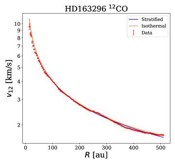
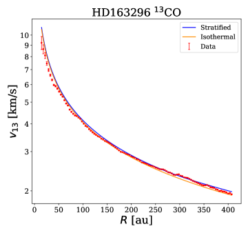
Figure 7: Same as Fig. 4 but for HD 163296.

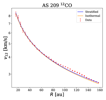
Figure 8: Same as Fig. 4 but for AS 209.

4.6 HD 163296

HD 163296 is one of the most well-studied Herbig Ae star system at millimeter wavelengths due to its relative close distance ($d=101$pc) and bright disk. The disk presents several features that suggest ongoing planet formation, as dust rings, deviations from Keplerian velocities due to gas pressure variations, ‘kinks’ in the CO emission, and meridional flows (Isella et al. 2016, 2018; Pinte et al. 2018; Teague et al. 2018; Pinte et al. 2023; Izquierdo et al. 2022; Calcino et al. 2022; Izquierdo et al. 2023).
This system has also been extensively studied because there are evidences of a massive disk. Powell et al. (2019) through modeling of dust lines found that the disk mass is $M_{d}=0.21\text{M}_{\odot}$. As for the scale radius, de Gregorio-Monsalvo et al. (2013) through radiative transfer modeling found that $R_{c}=125$au is the value that better reproduces dust and CO ALMA observations. Guidi et al. (2016) presented a multiwavelength ALMA and VLA study of the disk and through visibilities modeling found that the best fit value of the scale radius is $R_{c}=118$au, in agreement with de Gregorio-Monsalvo et al. (2013).

When we fit data with a vertical isothermal model, we obtain as the best fit parameters $M_{\star}=1.842\pm 0.002\text{M}_{\odot}$, $M_{d}=0.124\pm 0.001\text{M}_{\odot}$ and $R_{c}=38\pm 1$au. While the star mass is realistic, the scale radius is unrealistically small compared to the gas emission extent of the order of $400$au (Law et al. 2021). Additionally, the isothermal model is not able to reproduce the difference between the rotation curves of the two CO isotopologues (see Fig. 3), resulting in a relatively poor fit with a large $\chi^{2}_{\text{red}}$. If we include the 2D thermal structure, the quality of the fit increases (see $\chi^{2}_{\text{red}}$ in Table 2). In this case, the best fit for stellar mass and disk mass does not change significantly ($M_{\star}=1.948\pm 0.002M_{\odot},M_{\text{d}}=0.134\pm 0.001M_{\odot}$), while the scale radius does to $R_{c}=91\pm 1\text{au}$. Comparing our result for the disk mass to the literature values, we observe that our fit gives a value that is roughly half. Figure 7 shows that both the isothermal and the stratified model describe well the rotation curve of ¹²CO and ¹³CO. However, the shift between them, presented in Fig. 3, is well recovered only by the stratified model, which partially managed to explain the significant increase of the plotted quantity. The presence of pressure modulated substructures in the rotation curves (Izquierdo et al. 2023) impacts the quality of the fit and they are clearly visible in Fig. 3. A possible development would be to model them, including them in the fitting model.

4.7 AS 209

AS 209 is a young T-Tauri star in the Ophiucus star forming region ($d\sim 121$pc). The most recent stellar mass estimate is $M_{\star}=1.14\text{M}_{\odot}$ (Izquierdo et al. 2023). Fedele et al. (2018) gave an estimate for the scale radius $R_{c}=80$au through mm visibilities modeling. Afterwards, through thermochemical modeling, they found a dust mass of $M_{\text{dust}}=3.5\times 10^{-4}\text{M}_{\odot}$ that, with a gas-to-dust ratio of 100, translates into $M_{d}=0.0035\text{M}_{\odot}$, in agreement with the recent value $M_{d}=0.0045\text{M}_{\odot}$ of Zhang et al. (2021). Interestingly, when inspecting the rotation curves of AS 209 (Fig. 2), the ¹³CO is slower compared to the ¹²CO, despite it being closer to the midplane. This trend is observed up to $\sim 125$au. A possible explanation for this is the compactness of the disk, which makes more difficult to extract a precise emitting surface due to beam smearing. Indeed, line centroids from pixels near the center of the disk are an averaged composition of multiple surrounding velocities because of both the limited resolution and the steepness of v(r). Since AS209 is the smallest disk in the sample, it is more prone to be affected by that in a largest fraction of its total extent compared to the other sources. When we fit with the isothermal model, we obtain as the best fit parameters $M_{\star}=1.272\pm 0.003\text{M}_{\odot}$, $M_{d}=0.042\pm 0.003\text{M}_{\odot}$ and $R_{c}=45\pm 1$au. When we fit with the stratified model, we obtain as the best fit parameters $M_{\star}=1.311\pm 0.001\text{M}_{\odot}$, and $R_{c}=126\pm 2$au, while for the disk mass we report a $3-\sigma$ upper limit of $M_{d}=0.00025\pm 0.00025\text{M}_{\odot}$, since the best fit parameter is compatible with zero. In Fig. 8 both models are shown. As for ¹²CO, the two models behave in the same way, showing little difference in the outer edge. Conversely, for ¹³CO the isothermal model works better in the inner part, where ¹³CO is slower, while in the outer part the stratified model describes well the rotation curve. According to the $\chi^{2}_{\text{red}}$, the stratified model describes better the data (see Table 2).

Table 2: Results of the fitting procedure and reduced chi-squared for the two different models: isothermal and stratified.

	$M_{\star}$ [M⊙]	$M_{d}$ [M⊙]	$R_{c}$ [au]	$\chi^{2}_{\text{red}}$
MWC 480
Isothermal	1.969 $\pm 0.002$	0.201$\pm 0.002$	80$\pm 1$	11.21
Stratified	2.027$\pm 0.002$	$0.150\pm 0.002$	128 $\pm 1$	6.14
IM Lup
Isothermal	1.055 $\pm 0.002$	0.200$\pm 0.003$	55$\pm 1$	35.68
Stratified	1.194$\pm 0.002$	$0.106\pm 0.002$	115 $\pm 1$	6.29
GM Aur
Isothermal	0.872 $\pm 0.003$	0.312$\pm 0.003$	56$\pm 1$	90.84
Stratified	1.128$\pm 0.002$	0.118$\pm 0.002$	96 $\pm 1$	8.48
HD 163296
Isothermal	1.842 $\pm 0.002$	0.124$\pm 0.001$	38$\pm 1$	29.60
Stratified	1.948$\pm 0.002$	$0.134\pm 0.001$	91 $\pm 1$	19.74
AS 209
Isothermal	1.272 $\pm 0.003$	0.042$\pm 0.003$	45$\pm 1$	25.13
Stratified	1.311$\pm 0.001$	$0.0002\pm 0.0002$	126 $\pm 2$	10.55

5 Discussion

5.1 Thermal stratification in MAPS disks

Table 2 presents a summary of the findings of this study, comparing the isothermal model with the stratified one. It is evident from the results that the reduced $\chi^{2}$ value consistently decreases when employing the stratified model. This indicates that the inclusion of thermal stratification provides a more effective way of describing the observed data. In this context, MWC 480 is particularly interesting. Despite the small kinematic signatures of thermal stratification, as depicted in Fig. 3, the quality of the stratified fit is higher and it yields more reliable values for star mass, disk mass, and scale radius. On the opposite side, GM Aur is the system that shows the strongest effects of thermal stratification, being the ¹²CO and ¹³CO systematically shifted over all the radial extent of the disk. The introduction of thermal stratification is able to reconcile these differences, reducing by an order of magnitude the $\chi^{2}_{\text{red}}$. The only case where the stratified model encounters challenges in accurately describing both curves is AS 209. This system is peculiar because the compactness of the disk influences the extraction of emission surfaces. Consequently, contrary to what expected, we observe that the ¹³CO rotates slower than the ¹²CO in the inner part. Despite that, the $\chi^{2}_{\text{red}}$ is smaller when thermal stratification is taken into account.

5.2 Disk masses

In this paragraph, we aim to contextualize our work within the broader framework of disk mass estimation.

One solid tracer of the disk mass is the carbon dioxide HD. HD is a good tracer of disk gas because it follows the distribution of molecular hydrogen and its emission is sensitive to the total mass. The first detection of HD emission in a protoplanetary disk comes from Bergin et al. (2013) for TW Hya. Afterwards, the detection of HD $J=1-0$ line has been used to estimate disk mass of GM Aur. The HD based disk mass is $2.5-20.4\times 10^{-2}\text{M}_{\odot}$ (McClure et al. 2016), in line with our estimate of 0.118M_⊙. Finally, the non-detection of HD in HD163296 (Kama et al. 2020) translates into an upper limit for the disk mass of $0.067\text{M}_{\odot}$, that is almost half of the value we obtained in this work.

Another reliable method to trace the disk mass uses the N₂H⁺. This molecule is a chemical tracer of CO-poor gas and can be used to measure the CO-H₂ ratio and calibrate CO-based gas masses. Combining N₂H⁺ with C¹⁸O, Trapman et al. (2022) estimated disk masses of three protoplanetary disks, including GM Aur. The value they obtained is $1.5-9.6\times 10^{-2}\text{M}_{\odot}$, slightly higher compared to our estimate, but in an overall good agreement. This method has also been used to probe disk masses of protoplanetary disks in the Lupus star forming region (Anderson et al. 2022).

In this context, it is worth mentioning observations of the ¹³C¹⁷O, a very rare CO isotopologue. Booth et al. (2019) observed this molecule in HD 163296 and this allows to give precise disk mass measurement. They found that the disk mass that better reproduces observations is $M_{d}=0.31\text{M}_{\odot}$. discrepancy with out inferred value.

As for the dust, its ability of tracing mass is discussed in the next paragraph.

5.3 Gas-to-dust ratio

With the knowledge of the disk mass, it is possible to evaluate the gas-to-dust ratio, using Eq. (25) for the dust mass. The results are shown in Table 3, and we found values between $100-250$, within only a factor of 2 from the usually assumed valued of 100. This is surprisingly, due to the several assumptions we made to obtain the dust mass. Indeed, as we have already mentioned, the optically thin hypothesis for dust emission could lead to a difference of a more than a factor 2 in the dust mass calculation (Guidi et al. 2016), underestimating it. In addition, the dust opacity could also vary of a factor $\sim 10$ depending on the grain size and composition. Hence, overall, it is significant that the inferred gas-to-dust ratio is so close to the standard value. As for AS 209, we estimate an upper limit for this quantity. Indeed, according to Veronesi et al. (in prep), the minimum measurable mass with the rotation curve is 5% of the star mass. Taking this value as an upper limit for AS 209 disk mass, it is possible to give an upper limit for the gas-to-dust ratio.

Table 3: Continuum fluxes at 283 GHz, dust masses from eq. (25) and gas-to-dust ratio using the best fit value of the disk mass of the stratified model.

	$F_{283}$ [mJy]	$M_{\text{dust}}$ [M⊙]	Gas-to-dust ratio
MWC 480	943.51	0.00138	108
IM Lup	536.25	0.00075	134
GM Aur	347.95	0.00049	240
HD 163296	1127.97	0.00064	202
AS 209	414.83	0.00034	¡ 192

5.4 Toomre Q

In order to investigate the presence of gravitational instability we use our best fit parameters for the stratified model to compute the Toomre parameter (Toomre 1964) which, in the hypothesis of nearly Keplerian disk ($\kappa\simeq\Omega$), is

$$Q\simeq\frac{c_{\text{s}}\Omega}{\pi G\Sigma}=2\left.\frac{H}{R}\right|_{\text{mid}}\frac{M_{\star}}{M_{d}}\left(\frac{R}{R_{c}}\right)^{-1}\exp\left[\frac{R}{R_{c}}\right],$$ (26)

where we used Eq. (1) for the surface density. According to the WKB quadratic dispersion relation (Lin & Shu 1964; Toomre 1964), the onset of the instability happens when $Q\sim 1$. Figure 9 shows the profile of the Q parameter for the MAPS sample, except for AS209, since its disk mass estimate is compatible with zero. Every disk is gravitationally stable, according to the Toomre criterion, since $Q>1$. Interestingly, the two disks that shows spiral structures (IM Lup and GM Aur), have the Toomre profile lower compared to the others, with a minimum value of $\sim 4$ for GM Aur and $\sim 6$ for IM Lup. Lau & Bertin (1978) showed that a WKB description of gravitational instability can still be obtained under less restrictive conditions compared to the quadratic relation and they showed that disks that are locally stable according to the Q criterion might still generate large scale spiral waves. In general, other mechanisms could increase the critical value of the Toomre parameter, such as external irradiation (Lin & Kratter 2016; Löhnert et al. 2020) or dust driven gravitational instability (Longarini et al. 2023b, a). Hence, we do not exclude that gravitational instability is at play in GM Aur and IM Lup.

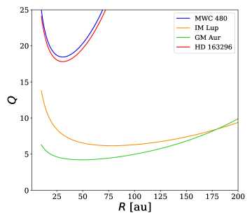
Figure 9: Toomre Q parameter of the MAPS disks with the best fit parameters of the stratified model. We excluded AS 209 because its best fit disk mass is compatible with zero.

6 Conclusions

Kinematic data of protoplanetary disks show velocity differences between ¹²CO and ¹³CO that cannot be explained through a vertically isothermal model, given the systematic shift between rotation curves of CO isotopologues. In this work, we predict how thermal stratification affects the density and the velocity field of a protoplanetary disk. We use SPH simulations to test our model, finding excellent agreement, and then we apply it to the MAPS sample. We extract rotation curve of CO isotopologues (¹²CO and ¹³CO) and we fit for star mass, disk mass and scale radius both with a vertically isothermal and a stratified model. The quality of the fit significantly improves when thermal stratification is taken into account and the best fit parameter are more realistic and aligned with literature. All the results are summarised in Table 2.

Typically, when thermal stratification is considered, the best fit value for the star mass tends to rise. This can be intuitively understood, as an isothermal model would favor a star mass that lies between that of ¹³CO and ¹²CO, in this way underestimating it due to the slower rotation of ¹²CO. Conversely, the stratified model encapsulates the difference between the two curves, mitigating the underestimation issue and resulting in a more accurate mass estimate. While an isothermal model provides a satisfactory fit at small radii, the fit worsens at large radii where the difference between ¹²CO and ¹³CO is larger. The fit tries to compensate for this by increasing the disk mass, most of which resides at large radii, thereby changing the predicted curve only in the outer parts of the disk. Ultimately, a more accurate description of the thermal structure through a stratified model leads to a realistic estimate of the scale radius.

We note that the inclusion of the vertical gradient of temperature into our model results in improved $\chi^{2}$ values across all systems under examination. This work demonstrates the impact of thermal stratification in the disk dynamics and highlights the importance of having a precise knowledge of the disk temperature structure to infer physical quantities such as the stellar mass, the disk mass and the disk scale radius in a meaningful manner. Thanks to the generality of our calculations, we can study the density and velocity profile of thermally stratified disk according different prescription of temperature simply.

Appendix A Computing the pressure gradient

Assuming a barotropic fluid, the pressure contribution to the rotation curve is

$$\frac{R}{\rho}\frac{dP}{dR}\Bigg{|}_{z}=\frac{R}{\rho}\Bigg{(}c_{\text{s}}^{2}\frac{d\rho}{dR}\Bigg{|}_{z}+\rho\frac{dc_{\text{s}}^{2}}{dR}\Bigg{|}_{z}\Bigg{)},$$ (27)

which can be written as

$$\begin{split}\frac{R}{\rho}\frac{dP}{dR}\Bigg{|}_{z}=c_{\text{s}}^{2}\frac{R}{\rho_{\text{mid}}g}&\Bigg{(}\rho_{\text{mid}}\frac{dg}{dR}\Bigg{|}_{z}+g\frac{d\rho_{\text{mid}}}{dR}\Bigg{|}_{z}\Bigg{)}+\\ R&\Bigg{(}c_{\text{s,mid}}^{2}\frac{df}{dR}\Bigg{|}_{z}+f\frac{dc_{\text{s,mid}}^{2}}{dR}\Bigg{|}_{z}\Bigg{)}=\\ c_{\text{s}}^{2}\Bigg{[}-\gamma^{\prime}&-(2-\gamma)\left(\frac{R}{R_{c}}\right)^{2-\gamma}+R\frac{d\log(fg)}{dR}\Bigg{|}_{z}\Bigg{]}.\end{split}$$ (28)

Assuming hydrostatic equilibrium in the vertical direction, we can write an explicit expression for the last term in Eq.(28):

$$\begin{split}-\Omega_{\text{k}}^{2}z\left[1+\left(\frac{z}{R}\right)^{2}\right]^{-3/2}&=-\frac{d\Phi_{\star}}{dz}=\frac{1}{\rho}\frac{dP}{dz}=\\ \frac{1}{\rho}P_{\text{mid}}\frac{d(fg)}{dz}&=c_{\text{s,mid}}^{2}f\frac{d\log(fg)}{dz}\end{split}$$ (29)

and, assuming $f(z=0)=1$ (therefore $T(R,z=0)=T_{\text{mid}}(R))$,

$$\log(fg)=-\frac{1}{H_{\text{mid}}^{2}}\int_{0}^{z}\frac{z^{\prime}}{f}\left[1+\left(\frac{z^{\prime}}{R}\right)^{2}\right]^{-3/2}dz^{\prime}.$$ (30)

Deriving with respect to R we obtain:

$$\begin{split}&R\frac{d\log(fg)}{dR}\Bigg{|}_{z}=R\Bigg{[}\frac{2}{H_{\text{mid}}^{3}}\frac{dH_{\text{mid}}}{dR}\int_{0}^{z}\frac{1}{f}\frac{z^{\prime}dz^{\prime}}{\Big{(}1+(z^{\prime}/R)^{2}\Big{)}^{3/2}}+\\ &\frac{1}{H_{\text{mid}}^{2}}\int_{0}^{z}\frac{1}{f^{2}}\frac{df}{dR}\frac{z^{\prime}dz^{\prime}}{\Big{(}1+(z^{\prime}/R)^{2}\Big{)}^{3/2}}-\frac{1}{H_{\text{mid}}^{2}}\int_{0}^{z}\frac{1}{f}\frac{3z^{\prime 3}/R^{3}dz^{\prime}}{\Big{(}1+(z^{\prime}/R)^{2}\Big{)}^{5/2}}\Bigg{]}=\\ &-\frac{q}{H_{\text{mid}}^{2}}\int_{0}^{z}\frac{1}{f}\frac{z^{\prime}dz^{\prime}}{(1+z^{\prime 2}/R^{2})^{3/2}}+\frac{R}{H_{\text{mid}}^{2}}\int_{0}^{z}\frac{\dot{f}}{f^{2}}\frac{z^{\prime}dz^{\prime}}{(1+z^{\prime 2}/R^{2})^{3/2}}+\\ &\frac{3}{H_{\text{mid}}^{2}}\int_{0}^{z}\frac{1}{f}\frac{z^{\prime}dz^{\prime}}{(1+z^{\prime 2}/R^{2})^{5/2}},\end{split}$$ (31)

where $\cdot=d/dR$. Expanding the logarithmic term is useful since it is now clear that the azimuthal velocity depends both on the temperature $(f)$ and on the temperature gradient $(\dot{f})$ along the radial direction. Moreover, it is easy to see the contribution of the vertical thermal stratification: in our model $f$ and $\dot{f}$ are function of $z$ and thus they have to be integrated to compute azimuthal velocity, while in vertically isothermal model this does not happen since $f=1$ and $\dot{f}=0$. We note that it is not analytically possible to determine generally the sign of Eq. (LABEL:derivlog) and thus the effect on the pressure gradient. However, for all the considered cases it never overcomes the gravitational contribution and leads to a faster deceleration in the rotation.

Appendix B Dullemond prescription

According to Law et al. (2021), the temperature prescription given by Dullemond et al. (2020) (Eq.(19)) fits well the data, but we note that in this case $f(R,z=0)\neq 1$ and the temperature does not smoothly connect to its value at midplane since $T(R,z=0)\neq T_{\text{mid}}(R)$. In order to evaluate this discrepancy, considering $T_{\epsilon}(R)\approx T_{\text{mid}}(R)$, we compute

$$\begin{split}\Delta(R)&=1-\frac{T(R,0)}{T_{\text{mid}}}=1-f(R,z=0)\approx\\ &-\frac{1}{8}\Bigg{(}\frac{T_{\text{atm}}}{T_{\text{mid}}}\Bigg{)}^{4}(R)(1-\tanh\alpha)=\\ &-\frac{1}{8}\Bigg{(}\frac{T_{\text{atm},100}}{T_{\text{mid},100}}\Bigg{)}^{4}\Bigg{(}\frac{R}{100\text{au}}\Bigg{)}^{-4(q_{\text{atm}}-q)}(1-\tanh\alpha),\end{split}$$ (32)

which is strongly dependent on $T_{\text{mid}},T_{\text{atm}}$ and $\alpha$. As shown in Table 4, the deviation of the actual midplane temperature from $T(R,z=0)$ as computed from the prescription given by Dullemond et al. (2020) is $\lesssim 10\%$ in our regions of interest ($R>100$au). This discrepancy could have relevance for systems such as GM Aur, HD 163296 and MWC 480. To examine this further, we conducted fits for these systems using both $T_{\text{mid}}(R)$ and $T(R,z=0)$ as the midplane temperature, and it was observed that this choice does not significantly alter the results. Thus, $T_{\text{mid}}\approx T(T,z=0)$ and $f(R,z=0)\approx 1$ and we can consider Eqs. (19) and (20) as a good parameterization for the temperature.

Table 4: Values of parameters used in the estimate (32).

	$(T_{\text{atm}}/T_{\text{mid}})_{100}$	$q_{\text{atm}}-q$	$\alpha$	$|\Delta(R=100$au)—
IM Lup	$1.44$	$0.05$	$4.91$	$5.8\cdot 10^{-5}$
GM Aur	$2.4$	$0.54$	$2.57$	$4.8\cdot 10^{-2}$
AS 209	$1.48$	$0.41$	$3.31$	$1.6\cdot 10^{-3}$
HD 163296	$2.63$	$0.43$	$3.01$	$2.9\cdot 10^{-2}$
MWC 480	$2.56$	$0.47$	$2.78$	$4.1\cdot 10^{-2}$

Appendix C Corner plots

In Figs 10 and 11 we present the corner plots of the MCMC fitting procedure for the studied parameters under, respectively, the vertically isothermal and the stratified model.

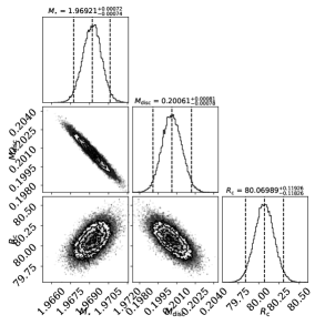
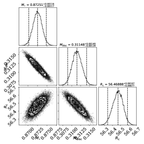
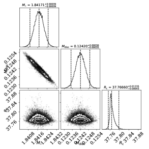
Figure 10: Corner plots of the MCMC fitting procedure according the vertically isothermal model. They show the distribution of the three relevant fitting parameters for the five disks of the MAPS large program. From top left to bottom: MWC 480, IM Lup, GM Aur, HD 163296 and AS 209.

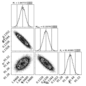
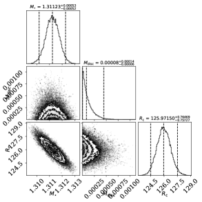
Figure 11: Corner plots of the MCMC fitting procedure according the stratified model. They show the distribution of the three relevant fitting parameters for the five disks of the MAPS large program. From top left to bottom: MWC 480, IM Lup, GM Aur, HD 163296 and AS 209.